Leptoquark-Mediated Two-Loop Neutrino Mass in Unified Theory

Abstract

Scalar leptoquarks naturally arise within unified theories, offering a promising avenue for addressing one of the most significant challenges of the Standard Model–the existence of non-zero neutrino masses. In this work, we present a unified theory based on the SU(5) gauge group, where neutrino mass appears at the two-loop level via the propagation of scalar leptoquarks. Due to the unified framework, the charged fermion and neutrino masses and mixings are entangled and determined by a common set of Yukawa couplings. These exotic particles not only shed light on the neutrino mass generation mechanism but also help achieve the unification of gauge couplings and are expected to lead to substantial lepton flavor violating rates, offering tangible opportunities for experimental verification. Reproducing the observed neutrino mass scale necessitates that leptoquarks reside a few orders of magnitude below the unification scale–a specific feature of the proposed scenario. Moreover, maximizing the unification scale implies TeV scale new physics states, making them accessible at colliders. The diverse roles that leptoquarks play highlight the elegance and predictive ability of the proposed unified model.

I Introduction

So far, the Standard Model (SM) of particle physics has proven to be extremely successful in reproducing many experimental observations. Despite its triumphs, the SM predicts massless neutrinos, whereas neutrino oscillations have been experimentally confirmed. Therefore, the SM clearly requires an extension. In the quest to find an ultraviolet-complete theory beyond the SM, Grand Unified Theories Pati:1973rp ; Pati:1974yy ; Georgi:1974sy ; Georgi:1974yf ; Georgi:1974my ; Fritzsch:1974nn (GUTs) have emerged as the most attractive scenarios. The SU(5) GUT, proposed in the early 1970s by Georgi and Glashow Georgi:1974sy , represents a significant step towards unifying the fundamental forces of nature. This unified framework has a number of appealing features, such as the merging of electromagnetic, weak, and strong nuclear forces into a single force at high energy levels; the unification of quarks with leptons; and the prediction of the existence of superheavy gauge bosons that mediate nucleon decays—a smoking-gun signature of GUTs.

However, the Georgi-Glashow model’s simplicity, characterized by the inclusion of only an adjoint Higgs, $24_{H}$, for GUT symmetry breaking and a fundamental Higgs, $5_{H}$, for electroweak symmetry breaking, renders it incompatible with experimental findings. Specifically, the model falls short in several key areas: (i) it fails to achieve unification of gauge couplings, (ii) it results in a mass degeneracy between down-type quarks and charged leptons, which is inconsistent with observed data, and (iii) it does not provide a mechanism for incorporating neutrino masses.

Within the renormalizable scheme, one of the simplest options to restore gauge coupling unification, saving the theory from too rapid proton decay, as well as correcting the bad mass relations between the charged leptons and down-type quarks can be achieved by extending the Georgi-Glashow model by adding just a single Higgs in the $45_{H}$ dimensional representation. In this framework, neutrinos, however remain massless. There have been numerous efforts to endow neutrinos with non-zero masses (see, for example, Refs. Dorsner:2005fq ; Dorsner:2005ii ; Bajc:2006ia ; Dorsner:2006hw ; Dorsner:2007fy ; Antusch:2021yqe ; Antusch:2022afk ; Calibbi:2022wko ; Antusch:2023kli ; Antusch:2023mqe , where neutrinos get their masses at the tree-level, and Refs. Wolfenstein:1980sf ; Barbieri:1981yw ; Perez:2016qbo ; Kumericki:2017sfc ; Saad:2019vjo ; Klein:2019jgb ; Dorsner:2019vgf ; Dorsner:2021qwg ; Antusch:2023jok ; Dorsner:2024jiy , where neutrino masses appear at the loop level).

By observing the crucial fact that $5_{H}$ and $45_{H}$ multiplets already contain a number of scalar leptoquarks, in this work, we propose a two-loop neutrino mass mechanism by an economical extension of this framework. More specifically, we add a $40_{H}$ dimensional scalar field, submultiplets of which, following electroweak symmetry breaking, mix with leptoquarks contained within $5_{H}$ and $45_{H}$. This mixing facilitates interactions between leptons and quarks for some of the submultiplets of $40_{H}$, allowing neutrinos to acquire mass via quantum corrections. Intriguingly, in the last several years, leptoquarks have gained a lot of attention in the particle physics community due to their ability to address multiple flavor anomalies that include the longstanding tension in the muon anomalous magnetic moment.

It is interesting to point out that within the proposed setup, the masses of the charged fermions and neutrinos are intertwined and governed by a common set of original Yukawa interactions. We find that to correctly reproduce the neutrino mass scale, leptoquarks running inside the loop must have masses $M_{\mathrm{LQ}}\lesssim 10^{8}$ GeV. However, in general, some of these leptoquarks facilitate proton decay, which typically imposes a lower limit of $M_{\mathrm{LQ}}\gtrsim 10^{12}$ GeV. Therefore, consistently reproducing neutrino oscillation data demands a cancellation mechanism for proton decay channels–a specific feature of this model. Additionally, the Yukawa interactions tailored to fit the masses and mixings of charged fermions and neutrinos predict the occurrence of charged lepton flavor violating (cLFV) processes. These processes offer distinct avenues for experimental investigation. Current searches for cLFV significantly constrain the mass of leptoquarks involved in these processes to be above $M_{\mathrm{LQ}}\gtrsim 10^{5}$ GeV. Interestingly, to maximize the GUT scale, a set of new physics states that includes an iso-triplet, a color sextet, and a color octet scalar could potentially have masses close to the TeV range. This makes them accessible to exploration at present and forthcoming collider experiments, presenting an exciting frontier for experimental physics.

This article is organized in the following way. In Sec. II, we introduce the proposed model and derive the charged and neutral fermion masses and mixings matrices. In Sec. III, we describe gauge coupling unification, proton decay, and lepton flavor violation constraints. Moreover, a detailed numerical analysis taking into account fits to the charged fermion masses and mixings and neutrino oscillation data is also presented in Sec. III. Finally, we conclude in Sec. IV.

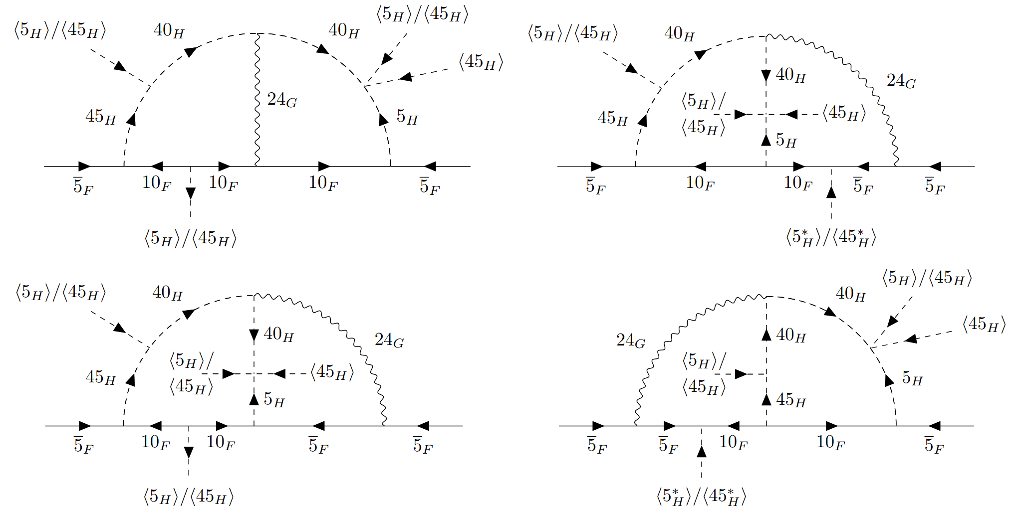
Figure 1: Example Feynman diagrams generating Majorana neutrino masses. See text for details.

II Model

In this section, we delve into the intricacies of the proposed model, specifically crafted to explain the phenomenon of neutrino oscillation. First, we describe how the bad mass relations between the down-type quarks and charged leptons are corrected within this framework. Subsequently, we provide a comprehensive exploration of the mechanisms underlying neutrino mass generation.

In an SU(5) GUT, all the SM fermions of each generation are contained in the following two fermionic representations:

$${\bm{\overline{5}_{F}}}_{i}=\ell_{i}(1,2,-\frac{1}{2})\oplus d_{i}^{c}(\overline{3},1,\frac{1}{3}),$$ (1)

$${\bm{10_{F}}}_{i}=q_{i}(3,2,\frac{1}{6})\oplus u_{i}^{c}(\overline{3},1,-\frac{2}{3})\oplus e_{i}^{c}(1,1,1),$$ (2)

where $i=1-3$ is the generation index. In this scheme, the GUT symmetry is first broken down to the SM gauge group by the adjoint representation, $24_{H}$, and finally, the electroweak symmetry breaking is assisted by $5_{H}+45_{H}$ Higgses:

$$SU(5) \xrightarrow[]{\langle 24_{H}\rangle}SU(3)_{C}\times SU(2)_{L}\times U(1)_{Y}$$ (3)

$$\xrightarrow[]{\langle 5_{H}\rangle,\langle 45_{H}\rangle}SU(3)_{C}\times U(1)_{\mathrm{em}}\;.$$ (4)

We define these scalar fields in the following way:

$$\bm{5_{H}}\equiv\phi =\phi_{1}(1,2,\frac{1}{2})\oplus\phi_{2}(3,1,-\frac{1}{3}),$$ (5)

$$\bm{24_{H}}\equiv\Phi =\Phi_{1}(1,1,0)\oplus\Phi_{2}(1,3,0)\oplus\Phi_{3}(8,1,0)$$

$$\oplus\Phi_{4}(3,2,-\frac{5}{6})\oplus\Phi_{5}(\overline{3},2,+\frac{5}{6}),$$ (6)

$$\bm{45_{H}}\equiv\Sigma =\Sigma_{1}(1,2,\frac{1}{2})\oplus\Sigma_{2}(3,1,-\frac{1}{3})\oplus\Sigma_{3}(\overline{3},1,\frac{4}{3})$$

$$\oplus\Sigma_{4}(\overline{3},2,-\frac{7}{6})\oplus\Sigma_{5}(3,3,-\frac{1}{3})$$

$$\oplus\Sigma_{6}(\overline{6},1,-\frac{1}{3})\oplus\Sigma_{7}(8,2,\frac{1}{2}).$$ (7)

Furthermore, the electroweak scale vacuum expectation values (vevs) are defined as $\langle 5_{H}\rangle=v_{5}/\sqrt{2}\left(0\;0\;0\;0\;1\right)^{T}$ and $\langle 45_{H}\rangle_{1}^{15}=\langle 45_{H}\rangle_{2}^{25}=\langle 45_{H}\rangle_{3}^{35}=-1/3\langle 45_{H}\rangle_{4}^{45}=v_{45}/(2\sqrt{6})$, with $\sqrt{v_{5}^{2}+v_{45}^{2}}=246$ GeV.

Charged fermion mass

With the fields given above, the complete Yukawa Lagrangian is given by Georgi:1979df

$$-\mathcal{L}_{Y} =Y_{A}10_{F}\overline{5}_{F}5^{*}_{H}+Y_{B}10_{F}10_{F}5_{H}$$

$$+Y_{C}10_{F}\overline{5}_{F}45^{*}_{H}+Y_{D}10_{F}10_{F}45_{H}\;.$$ (8)

Here, to avoid cluttering, we have suppressed the group as well as generation indices. Expanding the above Lagrangian and substituting electroweak scale vevs, the fermion masses, can be written as

$$\mathcal{L}\supset-u^{T}M_{U}u^{c}-d^{T}M_{D}d^{c}-e^{T}M_{E}e^{c}+\mathrm{h.c.}\,.$$ (9)

From Eq. (8), the charged fermion masses read Georgi:1979df ; Dorsner:2006dj

$$M_{D}=\frac{v_{5}}{2}Y_{A}-\frac{v_{45}}{2\sqrt{6}}Y_{C}\;,$$ (10)

$$M_{E}=\frac{v_{5}}{2}Y_{A}^{T}+\frac{\sqrt{3}v_{45}}{2\sqrt{2}}Y_{C}^{T}\;,$$ (11)

$$M_{U}=\sqrt{2}v_{5}\left(Y_{B}+Y_{B}^{T}\right)+\frac{v_{45}}{\sqrt{3}}\left(Y_{D}-Y_{D}^{T}\right)\;,$$ (12)

where $D,E,$ and $U$ represent down-type quark, charged lepton, and up-type quark sectors, respectively. Note that due to the additional contribution from $45_{H}$, the bad mass relation of the Georgi-Glashow model $M_{E}=M^{T}_{D}$ is broken, and $M_{U}$ is no longer a symmetric matrix. We bi-diagonalize these matrices with the help of unitary matrices as follows:

$$M_{U}=U_{L}M_{U}^{\mathrm{diag}}U_{R}^{\dagger}\,,$$ (13)

$$M_{D}=D_{L}M_{D}^{\mathrm{diag}}D_{R}^{\dagger}\,,$$ (14)

$$M_{E}=E_{L}M_{E}^{\mathrm{diag}}E_{R}^{\dagger}\,.$$ (15)

As we will show shortly, just like the charged fermions, the neutrino mass matrix is also determined by the same Yukawa couplings, namely $Y_{A},Y_{B},Y_{C},$ and $Y_{D}$, making this scenario more attractive and economical.

Neutrino mass

As aforementioned, the set of fields introduced in the preceding section cannot incorporate neutrino mass; further extension is needed. For that purpose, first observe that $5_{H}$ contains a scalar leptoquark $\phi_{2}(3,1,-\frac{1}{3})$, whereas $45_{H}$ contains four scalar leptoquarks, namely $\Sigma_{2}(3,1,-\frac{1}{3}),\Sigma_{3}(\overline{3},1,\frac{4}{3}),\Sigma_{4}(\overline{3},2,-\frac{7}{6})$, and $\Sigma_{5}(3,3,-\frac{1}{3})$. With this inspection, in aiming to address non-zero neutrino masses, we introduce the following scalar field:

$$\bm{40_{H}}\equiv\eta =\eta_{1}(1,2,-\frac{3}{2})\oplus\eta_{2}(\overline{3},1,-\frac{2}{3})\oplus\eta_{3}(3,2,\frac{1}{6})$$

$$\oplus\eta_{4}(\overline{3},3,-\frac{2}{3})\oplus\eta_{5}(\overline{6},2,\frac{1}{6})\oplus\eta_{6}(8,1,1).$$ (16)

Remarkably, $40_{H}$ contains submultiplets that share the same quantum numbers under the group $SU(3)_{C}\times U(1)_{\mathrm{em}}$ as in the leptoquarks residing in $5_{H}$ and $45_{H}$ Higgses. Consequently, the introduction of this field allows neutrinos to acquire masses at the two-loop order, as shown in Fig. 1 (only a set of example diagrams are presented).

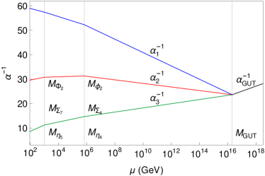
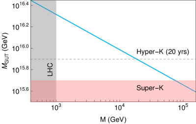
Figure 2: Left panel: Example of successful gauge coupling unification maximizing the GUT scale. Right panel: Maximal GUT scale as a function of the lightest intermediate-scale particle mass $M_{J}$. The lightest particle is either $\Phi_{2}$, $\Sigma_{7}$, or $\eta_{5}$. See text for details.

We emphasize that these Feynman diagrams are shown in the interaction basis. Neutrino mass must be computed in a basis where the fields running inside the loop are the physical states. Although in the flavor basis $\bm{40_{H}}$ has no Yukawa interactions, owing to electroweak symmetry breaking, its submultiplets $\eta_{2}(\overline{3},1,-\frac{2}{3}),\eta_{3}(3,2,\frac{1}{6})$, and $\eta_{4}(\overline{3},3,-\frac{2}{3})$ can, in general, mix with the rest of the leptoquarks (contained within $5_{H}$ and $45_{H}$ Higgses) with the right quantum numbers and gain lepton-quark interactions–resulting in non-zero neutrino mass. These desired mixings originate (see Fig. 1) from cubic couplings of the form

$$V\supset\mu_{1}45_{H}40^{*}_{H}5_{H}+\mu_{2}45_{H}40^{*}_{H}45_{H}\;,$$ (17)

and quartic couplings of the type

$$V \supset\lambda_{1}45_{H}40_{H}5_{H}5_{H}+\lambda_{2}45_{H}40_{H}5_{H}45_{H}$$

$$+\lambda_{3}45_{H}40_{H}45_{H}45_{H}\;.$$ (18)

As before, here, the group indices are suppressed. As can be seen from these two equations, mixings among leptoquarks are induced as a result of electroweak symmetry breaking.

Inside the loop, in addition to the $W^{\pm}$ gauge boson, two types of leptoquarks propagate, LQ^±1/3 and LQ^±2/3. The LQ^±1/3 (LQ^±2/3) states are, in general, a mixture of $\phi_{2},\Sigma_{2,5},\eta_{3,4}$ ($\Sigma_{4,5},\eta_{3,4}$) fields. Due to the presence of a large number of mixed leptoquarks, an analysis of the entire parameter space is somewhat challenging. We, therefore, make a simplified assumption that submultiplets $\phi_{2}\subset 5_{H}$, $\Sigma_{4}\subset 45_{H}$, and $\eta_{4}\subset 40_{H}$ reside below the GUT scale and contribute to the neutrino mass generation. The rest of the above mentioned leptoquarks are set to the GUT scale (alternatively, if light, their mixings are assumed to be tiny), hence provide completely negligible contribution to the neutrino masses. The electric charges of the $SU(2)_{L}$ iso-singlet, iso-doublet, and iso-triplet leptoquarks are $\phi_{2}^{-1/3}$, $\Sigma_{4}^{-5/3,-2/3}$, and $\eta_{4}^{-5/3,-2/3,+1/3}$, respectively, and we denote the corresponding physical states by $\chi^{\pm Q}_{a}$, where $Q=1/3,2/3,5/3$ and $a=1,2$.

As mentioned in the introduction, due to the unified nature of our proposal, the neutrino mass matrix is not arbitrary and, therefore, does not decouple from the charged fermion masses and mixings. By deriving the neutrino mass matrix, we find

$$M_{N} =NM_{N}^{\mathrm{diag}}N^{T}$$ (19)

$$=-\frac{3g^{2}}{\sqrt{2}\left(16\pi^{2}\right)^{2}}\bigg{\{}2Y^{T}_{L}M_{U}^{\mathrm{diag}}F_{L}+M_{E}^{\mathrm{diag}}Y^{\dagger}_{R}F_{L}$$

$$+M_{E}^{\mathrm{diag}}Y^{T}_{L}F_{R}^{*}\bigg{\}}J_{0}+\mathrm{(transpose)}\;.$$ (20)

These different contributions are written with the same loop function, $J_{0}$, which is valid in the limit when all SM fermion masses can be neglected (this is an excellent approximation since the leptoquarks are much heavier than the SM particles). In the above equation, we have defined

$$Y_{L}=U^{\dagger}_{L}\left(\frac{-Y_{A}}{\sqrt{2}}\right)E^{*}_{L},$$ (21)

$$Y_{R}=U^{T}_{R}\left(2(Y^{T}_{B}+Y_{B})\right)E_{R},$$ (22)

$$F_{L}=U^{T}_{R}\left(Y_{C}\right)E^{*}_{L},$$ (23)

$$F_{R}=U^{\dagger}_{L}\left(\sqrt{2}(-Y^{T}_{D}+Y_{D})\right)E_{R}\;.$$ (24)

Since we compute the neutrino mass in the charged lepton mass diagonal basis, $N=U_{\mathrm{PMNS}}$ is the Pontecorvo–Maki–Nakagawa–Sakata (PMNS) matrix. The loop factor $J_{0}$ in the limit when all the charged fermion masses can be neglected is given by Julio:2022ton ; Julio:2022bue

$$J_{0}=\frac{1}{4}\sin 2\theta\sin 2\phi\sum_{a,b=1}^{2}(-1)^{a+b}J(M_{a+2},M_{b}).$$ (25)

Here, $\theta$ and $\phi$ represent the mixing angles of leptoquarks with electric charges $1/3$ and $2/3$, respectively. Moreover, $M_{1,2}$ are masses for $2/3$ charged and $M_{3,4}$ are for $1/3$ charged leptoquarks. Finally, $J$ is defined in the following way:

$$J(M_{a+2},M_{b})=8\left(1-\frac{3}{4}\frac{M_{a+2}}{M_{b}}\right)-\frac{5\pi^{2}}{6}\left(1-\frac{2}{5}\frac{M_{a+2}}{M_{b}}\right)$$

$$+\frac{M_{b}^{2}}{m_{W}^{2}}\left(\frac{M_{a+2}}{M_{b}}-1\right)\left(2-\frac{\pi^{2}}{3}\right)+\left(\frac{2M_{a+2}}{M_{b}}-1\right)\ln\frac{m_{W}^{2}}{M_{b}^{2}},$$ (26)

which is valid in the regime of our interest, namely $M_{b}/M_{a+2}-1\ll 1$.

III Results

In this section, we describe how gauge coupling unification is achieved and examine proton decay and lepton flavor violation appearing in the proposed model. After discussing these issues, we carry out a detailed numerical analysis, including a fit to the fermion masses and mixings.

Gauge coupling unification

The one-loop running of the SM gauge couplings ($\alpha_{i}=g_{i}^{2}/(4\pi)$) is given by

$$\alpha_{i}^{-1}(M_{Z})=\alpha_{\textrm{GUT}}^{-1}-\frac{b_{i}^{\textrm{SM}}\ln(\frac{M_{\textrm{GUT}}}{M_{Z}})}{2\pi}-\sum_{J}\frac{b_{i}^{J}\ln(\frac{M_{\textrm{GUT}}}{M_{J}})}{2\pi},$$ (27)

where $b_{i}^{\textrm{SM}}$ are the SM one-loop gauge coefficients, while $b_{i}^{J}$ denote the one-loop gauge coefficients of intermediate-scale particles with masses $M_{J}$, such that $M_{Z}\leq M_{J}\leq M_{\textrm{GUT}}$. We take the experimental low energy values of the gauge couplings from Ref. Antusch:2013jca . Assuming that the leptoquarks that contribute dominantly to neutrino mass, namely $\phi_{2},\Sigma_{4},$ and $\eta_{4}$, have nearly degenerate masses around $M_{\mathrm{LQ}}$, we study a minimal scenario, where we freely vary the masses $M_{\Phi_{2}},M_{\Sigma_{7}},M_{\eta_{5}},$ and $M_{\mathrm{LQ}}$ and let the other states reside at the GUT scale. Then, the following relations between the intermediate-scale particle masses and the GUT scal can be derived from Eq. (27):

$$M_{\mathrm{GUT}}=\sqrt[\scriptstyle 82]{\frac{M_{Z}^{109}}{M_{\Phi_{2}}^{5}M_{\Sigma_{7}}^{8}M_{\eta_{5}}^{14}}}\exp\left[\frac{15\pi}{41}\left(-\alpha_{2}^{-1}(M_{Z})+\alpha_{3}^{-1}(M_{Z})\right)\right],$$ (28)

$$M_{\mathrm{LQ}}=\sqrt[\scriptstyle 123]{\frac{M_{Z}^{158}M_{\Sigma_{7}}^{20}}{M_{\Phi_{2}}^{49}M_{\eta_{5}}^{6}}}\exp\left[\pi\left(\frac{4}{3}\alpha_{1}^{-1}(M_{Z})-\frac{98}{41}\alpha_{2}^{-1}(M_{Z})+\frac{130}{123}\alpha_{3}^{-1}(M_{Z})\right)\right].$$ (29)

We freely vary the masses $M_{\Phi_{2}},M_{\Sigma_{7}},$ and $M_{\eta_{5}}$ between the TeV (for the compatibility of the LHC bounds, a lower limit of 1 TeV has been taken) and the GUT scale, while taking an upper bound of $10^{8}$ GeV on $M_{\mathrm{LQ}}$ (which is needed to reproduce the correct neurino mass scale). Thereby, we find that gauge coupling unification can easily be achieved. One example for gauge coupling unification is presented in the left panel of Fig. 2. Moreover, the right panel of Fig. 2 shows how the maximal GUT scale depends on the smallest intermediate-scale particle mass $M$, where we have defined $M=\min\{M_{J}\}$. It turns out that in our study, the maximal GUT scale for a given $M$ is obtained for the scenario when $M=M_{\Phi_{2}}=M_{\Sigma_{7}}=M_{\eta_{5}}$. In particular, for $M=1$ TeV we find $M_{\textrm{GUT}}\leq 2.0\times 10^{16}$ GeV, which requires $M_{\mathrm{LQ}}$ to reside at 671 TeV. Also, gauge mediated proton decay roughly restricts the GUT scale to be above $M_{\textrm{GUT}}\gtrsim 5\times 10^{15}$ GeV. This, within the part of the parameter space we are exploring, gives a rough upper bound of $M\lesssim 75$ TeV. Hyper-Kamiokande–if it does not observe proton decay–will further reduce this scale to 18 TeV. If these states, namely the iso-triplet $\Phi_{2}(1,3,0)$, the color sextet $\Sigma_{7}(\overline{6},2,1/6)$ and color octet $\eta_{5}(8,2,1/2)$ reside close to the TeV scale, it opens up the possibility to search them at colliders.

Decay channel	Current bound	Future sensitivity
	$\tau_{p}$ [yrs]	$\tau_{p}$ [yrs]
$p\rightarrow K^{+}\,\overline{\nu}$	$8.0\times 10^{33}$ Okumura:2020xfs	$3.2\times 10^{34}$ Hyper-Kamiokande:2018ofw
$p\rightarrow\pi^{+}\,\overline{\nu}$	$3.9\times 10^{33}$ Super-Kamiokande:2013rwg	-
$p\rightarrow\pi^{0}\,e^{+}$	$2.4\times 10^{34}$ Super-Kamiokande:2020wjk	$7.8\times 10^{34}$ Hyper-Kamiokande:2018ofw
$p\rightarrow\pi^{0}\,\mu^{+}$	$1.6\times 10^{34}$ Super-Kamiokande:2020wjk	$7.7\times 10^{34}$ Hyper-Kamiokande:2018ofw
$p\rightarrow K^{0}\,e^{+}$	$1.1\times 10^{33}$ Brock:2012ogj	-
$p\rightarrow K^{0}\,\mu^{+}$	$3.6\times 10^{33}$ Super-Kamiokande:2022egr	-
$p\rightarrow\eta^{0}\,e^{+}$	$1.0\times 10^{34}$ Super-Kamiokande:2017gev	$4.3\times 10^{34}$ Hyper-Kamiokande:2018ofw
$p\rightarrow\eta^{0}\,\mu^{+}$	$4.7\times 10^{33}$ Super-Kamiokande:2017gev	$4.9\times 10^{34}$ Hyper-Kamiokande:2018ofw

Table 1: Current experimental bounds and future sensitivities (for 10 years of runtime) for different two-body proton decay channels.

Process	Present bound	Future sensitivity
BR($\mu\to e\gamma$)	$4.2\times 10^{-13}$ MEG:2016leq	$6\times 10^{-14}$ Baldini:2013ke
BR($\tau\to e\gamma$)	$3.3\times 10^{-8}$ BaBar:2009hkt	$\sim 10^{-9}$ Aushev:2010bq
BR($\tau\to\mu\gamma)$	$4.4\times 10^{-8}$ BaBar:2009hkt	$\sim 10^{-9}$ Aushev:2010bq
BR($\mu\to eee)$	$1.0\times 10^{-12}$ SINDRUM:1987nra	$\sim 10^{-16}$ Blondel:2013ia
BR($\tau\to eee)$	$2.7\times 10^{-8}$ Hayasaka:2010np	$\sim 10^{-9}$ Aushev:2010bq
BR($\tau\to\mu\mu\mu)$	$2.1\times 10^{-8}$ Hayasaka:2010np	$\sim 10^{-9}$ Aushev:2010bq
BR($\tau^{-}\to e^{-}\mu\mu$)	$2.7\times 10^{-8}$ Hayasaka:2010np	$\sim 10^{-9}$ Aushev:2010bq
BR($\tau^{-}\to\mu^{-}ee$)	$1.8\times 10^{-8}$ Hayasaka:2010np	$\sim 10^{-9}$ Aushev:2010bq
BR($\tau^{-}\to e^{+}\mu^{-}\mu^{-}$)	$1.7\times 10^{-8}$ Hayasaka:2010np	$\sim 10^{-9}$ Aushev:2010bq
BR($\tau^{-}\to\mu^{+}e^{-}e^{-}$)	$1.5\times 10^{-8}$ Hayasaka:2010np	$\sim 10^{-9}$ Aushev:2010bq
CR($\mu\textrm{Au}\to e\textrm{Au})$	$7\times 10^{-13}$ SINDRUMII:2006dvw	$-$
CR($\mu\textrm{Ti}\to e\textrm{Ti})$	$4.3\times 10^{-12}$ SINDRUMII:1993gxf	$\sim 10^{-18}$ unPUB
CR($\mu\textrm{Al}\to e\textrm{Al})$	$-$	$10^{-15}-10^{-18}$ Pezzullo:2017iqq

Table 2: Current experimental constraints and future sensitivities for various lepton violating processes; all at the 90% confidence level.

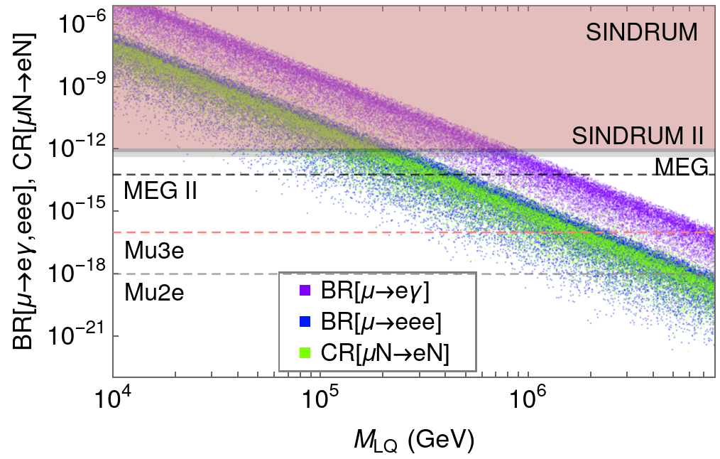
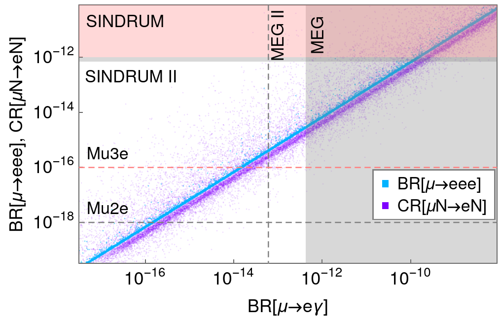
Figure 3: Left panel: Correlation between various cLFV processes and the LQ mass. Right panel: Correlation between various cLFV processes amongst each other. Current experimental constraints are represented by filled boxes, while future sensitivities are indicated by dashed lines. See text for details.

Proton decay

Proton decay is mediated by the usual superheavy gauge bosons $X(3,2,-5/6)$ and $\overline{X}(\overline{3},2,5/6)$. Among the scalars, a subset of leptoquarks–specifically $\phi_{2},\Sigma_{2},$ and $\Sigma_{5}$–play a direct role in facilitating dimension six proton decay. Additionally, $\eta_{3}$ and $\eta_{4}$ contribute through their electroweak mixing with other leptoquarks, as elaborated in the preceding discussion. Furthermore, $\Sigma_{3}$ can also lead to proton decays via loop-level contributions. In this work, we have performed an in-depth analysis of proton decay rates at the tree level. A comprehensive list of two-body proton decay widths mediated by gauge and scalar bosons, relevant Wilson coefficients, as well as long- and short-distance coefficients are presented in the Appendices A and B, respectively.

Note that in order to reproduce the correct neutrino masses, the masses of the leptoquarks $\phi_{2},\Sigma_{4},\eta_{4}$ running inside the loop should be below $M_{\mathrm{LQ}}\lesssim 10^{8}$ GeV. This is a requirement from both perturbativity of the Yukawa couplings as well as the needed orders of Yukawa couplings to replicate charged fermion masses. However, $\phi_{2}$ (and therefore the $(3,1,-1/3)$ component of $\eta_{4}$) mediates proton decay. This would without further suppression give a lower limit of $M_{\mathrm{LQ}}\gtrsim 10^{12}$ GeV on the mass of $\phi_{2}$ (more specifically, the states $\chi^{\pm 1/3}_{a}$). However, the proton decay contributions of $\chi^{\pm 1/3}_{a}$ can be fully rotated away in our model. The procedure to suppress proton decay using the freedom in the fermion mass matrices is widely known in the literature and has been studied, for example, in Refs. Nandi:1982ew ; Berezinsky:1983va ; Bajc:2002bv ; FileviezPerez:2004hn ; Dorsner:2004jj ; Dorsner:2004xa ; Dorsner:2005ii ; Dorsner:2005fq ; Nath:2006ut for the case of gauge boson mediated proton decay and in Refs. Nath:2006ut ; Dorsner:2012nq ; Dorsner:2012uz ; Fornal:2017xcj for the case of scalar mediated proton decay. Following these references, we adopt a similar approach. In particular, rotating away this corresponding proton decay contributions give the conditions Dorsner:2012nq $(U_{L}^{\dagger}(Y_{B}+Y_{B}^{T})D_{L}^{\ast})_{1\beta}=(D_{R}^{\dagger}Y_{A}^{\dagger}U_{R}^{\ast})_{\beta 1}=0$ for $\beta=1,2$, which we use for our numerical analysis. Finally, the current experimental constraints and future sensitivities for two-body proton decay channels are listed in Table 2.

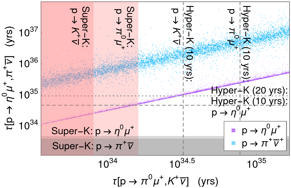
Figure 4: Left panel: Correlation between various proton decay channels. Right panel: Correlation between cLFV and proton decay. See text for details.

Lepton flavor violation

The Yukawa couplings Eqs. (21)-(24) that appear in the neutrino mass formula Eq. (20) naturally lead to lepton flavor violating processes. Among the three different types of leptoquarks, the couplings of $\chi^{\pm 1/3}$ and $\chi^{\pm 5/3}$ are severely constrained owing to chirality-enhanced lepton flavor violating processes as a result of the simultaneous presence of both left- and right-chiral interactions with fermions. On the other hand, cLFV processes lead by $\chi^{\pm 2/3}$ leptoquark are comparatively suppressed. In our analysis, we take into account all the important two-body and three-body decays $\ell_{\alpha}\to\ell_{\beta}\gamma$ and $\ell^{-}_{\alpha}\to\ell^{-}_{\beta}\ell^{-}_{\gamma}\ell^{+}_{\gamma}$, as well as $\mu\to e$ conversion in nuclei. For the computation of these processes, we follow Ref. Julio:2022ton and the references therein. Moreover, Table 2 summarizes all current experimental bounds and sensitives of upcoming experiments. As we will shown below, the present lepton flavor violating constraints typically put a lower bound of $M_{\mathrm{LQ}}\gtrsim 10^{5}$ GeV on the mass of the leptoquarks.

Numerical analysis and results

For our numerical analysis we work in the basis in which the charged lepton mass matrix is diagonal. We then parameterize the Yukawa matrices $Y_{A},Y_{C},(Y_{B}+Y_{B}^{T})$, and $(Y_{D}-Y_{D}^{T})$ in terms of the charged fermion masses and the unitary rotation matrices $U_{L},U_{R},D_{L}$, and $D_{R}$:

$$Y_{A}=\frac{1}{2v_{5}}\left(M_{E}^{\mathrm{diag}}+3D_{L}M_{D}^{\mathrm{diag}}D_{R}^{\dagger}\right),$$ (30)

$$Y_{C}=\frac{\sqrt{3}}{\sqrt{2}v_{45}}\left(M_{E}^{\mathrm{diag}}-D_{L}M_{D}^{\mathrm{diag}}D_{R}^{\dagger}\right),$$ (31)

$$Y_{B}+Y_{B}^{T}=\frac{1}{2\sqrt{2}v_{5}}\left(U_{L}M_{U}^{\mathrm{diag}}U_{R}^{\dagger}+U_{R}^{\ast}M_{U}^{\mathrm{diag}}U_{L}^{T}\right),$$ (32)

$$Y_{D}-Y_{D}^{T}=\frac{\sqrt{3}}{2v_{45}}\left(U_{L}M_{U}^{\mathrm{diag}}U_{R}^{\dagger}-U_{R}^{\ast}M_{U}^{\mathrm{diag}}U_{L}^{T}\right).$$ (33)

Note that we parametrize the up-type quark left-mixing rotation matrix as $U_{L}=D_{L}\textrm{diag}(e^{i\beta_{1}^{u}},e^{i\beta_{2}^{u}},1)V_{\mathrm{CKM}}^{T}$, where $V_{\mathrm{CKM}}$ is the Cabibbo-Kobayashi-Maskawa (CKM) matrix. This parametrization is derived by solving Eqs. (10)-(12) for the Yukawa matrices. It has the advantage that the charged fermion masses and CKM mixing angles can be used as input parameters (which we take from Ref. Babu:2016bmy ), hence these quantities do not require to be fitted. Therefore, we scan over the rest of the free parameters in the rotation matrices.

We use these free parameters together with the ones defined in Eq. (25) to fit the neutrino masses and PMNS mixings (we take the experimental values from Refs. Esteban:2020cvm ; NUFIT ), while making sure that all proton decay and cLFV constraints are satisfied, and while choosing the intermediate-scale particle masses such that the gauge couplings do unify. Using a differential evolution algorithm we compute 12 different benchmark points; all having a negligible total $\chi^{2}$. Starting from each benchmark point and applying an adaptive Metropolis-Hastings algorithm we perform a Markov-chain-Monte-Carlo (MCMC) analysis. For each chain we compute 1.5 million points giving us 18 million points in total.

It must be noted that we only find good fit points for the case of normal neutrino mass ordering. This can be understood from the fact that the neutrino mass matrix is highly correlated to the charged fermion mass matrices. Consequentially, the neutrino mass matrix mirrors the normal mass hierarchy of the mass matrices of the charged fermions.

We find the most constraining cLFV processes to be $\mu\rightarrow e\gamma$, $\mu\rightarrow eee$, and $\mu-e$ conversion in nuclei. We, therefore, present in Fig. 3 the correlation between these three processes and the leptoquark mass scale $M_{\mathrm{LQ}}$ (left panel) as well as the correlation of these three processes amongst each other (right panel). The current bound on the process $\mu\rightarrow e\gamma$ typically constrains $M_{\mathrm{LQ}}\gtrsim 10^{5}$ GeV. Future sensitivities on the processes $\mu\rightarrow eee$ and $\mu-e$ conversion in nuclei have the potential to increase this bound by an order of magnitude if experiments happen not to observe any cLFV process. Moreover, we find a high correlation between the cLFV processes $\mu\rightarrow e\gamma$ and $\mu\rightarrow eee$ that can be looked for in future searches. We find BR($\mu\rightarrow e\gamma$)/BR($\mu\rightarrow eee)$ to lie within $(108,173)$ at the 2$\sigma$ confidence level (see Fig. 3).

For the gauge mediated proton decay, we find the channels $p\rightarrow\pi^{0}\ell^{+}$ to be typically dominant. But also proton decay in the channels $p\rightarrow\eta\ell^{+}$ or $p\rightarrow K^{+}\overline{\nu}$ may be observed. Interestingly, we find a high correlation between the decay channels $p\rightarrow\pi^{0}\mu^{+}$ and $p\rightarrow\eta^{0}\mu^{+}$ that can be looked for at Hyper-Kamiokande. At the $2\sigma$ confidence level, we find the ratio of partial lifetimes $\tau(p\rightarrow\pi^{0}\mu^{+})/\tau(p\rightarrow\eta^{0}\mu^{+})$ to lie within $(0.12,0.33)$. This correlation is depicted in the left panel of Fig. 4.

In the case of proton decay mediated by the scalar leptoquark $\Sigma_{2}$, we find amongst the usual channels that the decays $p\rightarrow K^{0}\ell^{+}$ are enhanced and could be tested if $\Sigma_{2}$ resides around $10^{12}$ GeV. Considering the leptoquark $\Sigma_{5}$, the dominant decay channel is $p\rightarrow K^{+}\overline{\nu}$. It can be looked for if $\Sigma_{5}$ resides around $10^{12}$ GeV. Moreover, for $\Sigma_{5}$-mediated proton decay, we find a somewhat interesting correlation between the two decay channels with antineutrinos in the final state. We findings dictate that the ratio of partial lifetimes $\tau(p\rightarrow K^{+}\overline{\nu})/\tau(p\rightarrow\pi^{+}\overline{\nu})$ to be within $(0.0052,0.0467)$ at the $2\sigma$ confidence level. This correlation is visualized in the left panel of Fig. 4.

Moreover, in the minimal scenario, where we freely vary the masses $M_{\Phi_{2}},M_{\Sigma_{7}},M_{\eta_{5}},$ and $M_{\mathrm{LQ}}$ for a gauge coupling unification analysis, while assuming that all other states reside around the GUT scale, there is additional correlation between lepton flavor violating processes and gauge mediated proton decay. This is due to the fact that the GUT scale depends on the choice of the leptoquark mass scale, $M_{\mathrm{LQ}}$. We illustrate this correlation by considering the cLFV process muon to electron conversion in nuclei and the proton decay channel $p\rightarrow\pi^{0}e^{+}$ in the right panel of Fig. 4. Interestingly, if the leptoquark mass scale gets larger than $10^{7}$ GeV gauge mediated proton decay violates the present Super-Kamiokande bound. On the other hand, a leptoquark mass scale below $10^{5}$ GeV is ruled out by current cLFV constraints. If not observed, future sensitivities on cLFV processes have the potential to increase this bound on the leptoquark mass scale by an order of magnitude.

From our comprehensive analysis, we conclude that the proposed model has exciting feature through which it can be simultaneously tested by a synergy of low energy searches looking for proton decay and cLFV.

IV Conclusions

Scalar leptoquarks emerge as natural constituents within unified theories, providing a compelling solution to one of the Standard Model’s critical puzzles–the presence of non-zero neutrino masses. In this study, we proposed a SU(5) grand unified model, in which neutrino masses are generated at the two-loop level through scalar leptoquark propagation. This unified approach intricately links the masses and mixing of charged fermions and neutrinos, governed by a unified set of Yukawa interactions. These exotic particles not only illuminate the process behind neutrino mass generation but also contribute to the unification of gauge couplings and may result in significant rates of lepton flavor violation, opening distinct pathways for experimental verification. The masses of a set of leptoquarks are predicted to lie several orders of magnitude below the unification scale from the requirement of reproducing the correct neutrino mass scale. This prerequisite necessitates a mechanism to suppress proton decay rates that these states could potentially induce. Furthermore, to maximize the unification scale, new physics states such as color sextet and octet scalars should be at the TeV scale, placing them within reach of colliders. The diverse roles played by the leptoquarks highlight the elegance and predictive ability of the proposed unified model.

Appendix A Gauge mediated proton decay

The complete formula for the gauge mediated two-body proton decay widths are FileviezPerez:2004hn ; Nath:2006ut

$$\Gamma(p\to K^{+}\bar{\nu})=\frac{(m_{p}-m_{K^{+}})^{2}}{8\pi m_{p}^{3}}A_{L}^{2}\sum_{i}\left|A_{SR}\left<K^{+}\vphantom{(us)_{R}d_{L}p}\right|(us)_{R}d_{L}\left|p\vphantom{K^{+}(us)_{R}d_{L}}\right>c(\nu_{i},d,s^{c})+A_{SL}\left<K^{+}\vphantom{(ud)_{R}s_{L}p}\right|(ud)_{R}s_{L}\left|p\vphantom{K^{+}(ud)_{R}s_{L}}\right>c(\nu_{i},s,d^{c})\right|^{2}\;,$$ (34)

$$\Gamma(p\to\pi^{+}\bar{\nu})=\frac{(m_{p}-m_{\pi^{+}})^{2}}{8\pi m_{p}^{3}}A_{L}^{2}A_{SR}^{2}|\left<\pi^{+}\vphantom{(ud)_{R}d_{L}p}\right|(ud)_{R}d_{L}\left|p\vphantom{\pi^{+}(ud)_{R}d_{L}}\right>|^{2}\sum_{i}|c(\nu_{i},d,d^{c})|^{2}\;,$$ (35)

$$\Gamma(p\to\pi^{0}e^{+}_{\alpha})=\frac{(m_{p}-m_{\pi^{0}})^{2}}{8\pi m_{p}^{3}}A_{L}^{2}\left(A_{SL}^{2}|\langle\pi^{0}|(ud)_{L}u_{L}|p\rangle c(e_{\alpha}^{c},d)|^{2}+A_{SR}^{2}|\langle\pi^{0}|(ud)_{R}u_{L}|p\rangle c(e_{\alpha},d^{c})|^{2}\right),$$ (36)

$$\Gamma(p\to K^{0}e^{+}_{\alpha})=\frac{(m_{p}-m_{K^{0}})^{2}}{8\pi m_{p}^{3}}A_{L}^{2}\left(A_{SR}^{2}|\langle K^{0}|(us)_{R}u_{L}|p\rangle c(e_{\alpha},s^{c})|^{2}+A_{SL}^{2}|\langle K^{0}|(ud)_{L}u_{L}|p\rangle c(e_{\alpha}^{c},s)|^{2}\right),$$ (37)

$$\Gamma(p\to\eta e^{+}_{\alpha})=\frac{(m_{p}-m_{\eta})^{2}}{8\pi m_{p}^{3}}A_{L}^{2}\left(A_{SL}^{2}|\langle\eta|(ud)_{L}u_{L}|p\rangle c(e_{\alpha}^{c},d)|^{2}+A_{SR}^{2}|\langle\eta|(ud)_{R}u_{L}|p\rangle c(e_{\alpha},d^{c})|^{2}\right).$$ (38)

Here, $A_{L}=1.2$ denotes the long-range coefficient Nihei:1994tx , while $A_{SL(R)}$ are the short-distance coefficients defined as

$$A_{SL(R)}=\prod_{i=1,2,3}\prod_{I}^{M_{Z}\leq M_{I}\leq M_{\textrm{GUT}}}\left(\frac{\alpha_{i}(M_{I+1})}{\alpha_{i}(M_{I})}\right)^{\frac{\gamma_{L(R)i}}{b_{i}^{\textrm{SM}}+\sum_{J}^{M_{Z}\leq M_{J}\leq M_{\textrm{GUT}}}b_{i}^{J}}},\;\text{with $\gamma_{L(R)i}=\left(23(11)/20,9/4,2\right)$.}$$ (39)

Moreover, $m_{p}=938.33$ MeV, $m_{\pi}=134$ MeV, $m_{\eta}=548$ MeV, and $m_{K}=493.677$ MeV are the proton, pion, eta meson, and kaon mass, respectively. The coefficients are defined as Buras:1977yy ; Ellis:1979hy ; Wilczek:1979hc

$$c(e_{\alpha}^{c},d_{\beta})=\frac{g_{\textrm{GUT}}^{2}}{2M_{\textrm{GUT}}^{2}}\left((U_{R}^{\dagger}U_{L}^{\ast})_{11}(E_{R}^{\dagger}D_{L}^{\ast})_{\alpha\beta}+(E_{R}^{\dagger}U_{L}^{\ast})_{\alpha 1}(U_{R}^{\dagger}D_{L}^{\ast})_{1\beta}\right)\ ,$$ (40)

$$c(e_{\alpha},d^{c}_{\beta})=\frac{g_{\textrm{GUT}}^{2}}{2M_{\textrm{GUT}}^{2}}(U_{R}^{\dagger}U_{L}^{\ast})_{11}(E_{L}^{\dagger}D_{R}^{\ast})_{\alpha\beta}\ ,$$ (41)

$$c(\nu_{l},d_{\alpha},d^{c}_{\beta})=\frac{g_{\textrm{GUT}}^{2}}{2M_{\textrm{GUT}}^{2}}(U_{R}^{\dagger}D_{L}^{\ast})_{1\alpha}(D_{R}^{\dagger}N)_{\beta l}\ .$$ (42)

Finally, we take the matrix elements from Ref. Aoki:2017puj , e.g. $\left<\pi^{0}\vphantom{(ud)_{L}u_{L}p}\right|(ud)_{L}u_{L}\left|p\vphantom{\pi^{0}(ud)_{L}u_{L}}\right>=+0.134(5)(16)\text{ GeV}^{2}$.

Appendix B Scalar mediated proton decay

The decay widths for scalar mediated two-body proton decay read FileviezPerez:2004hn ; Nath:2006ut

$$\Gamma(p\to K^{+}\bar{\nu})=\frac{(m_{p}-m_{K^{+}})^{2}}{32\pi m_{p}^{3}}A_{L}^{2}\sum_{i}\left|A_{SL}\left(\langle K^{+}|(us)_{L}d_{L}|p\rangle a(s,d,\nu_{i})+\langle K^{+}|(ud)_{L}s_{L}|p\rangle a(d,s,\nu_{i})\right)\right.\$$

$$\hskip 142.26378pt\left.\ +\,A_{SR}\left(\langle K^{+}|(us)_{R}d_{L}|p\rangle a(d,s^{c},\nu_{i})+\langle K^{+}|(ud)_{R}s_{L}|p\rangle a(s,d^{c},\nu_{i})\right)\right|^{2}\;,$$ (43)

$$\Gamma(p\to\pi^{+}\bar{\nu})=\frac{(m_{p}-m_{\pi^{+}})^{2}}{32\pi m_{p}^{3}}A_{L}^{2}\sum_{i}\left|A_{SL}\left<\pi^{+}\vphantom{(ud)_{L}d_{L}p}\right|(ud)_{L}d_{L}\left|p\vphantom{\pi^{+}(ud)_{L}d_{L}}\right>a(d,d,\nu_{i})+A_{SR}\left<\pi^{+}\vphantom{(ud)_{R}d_{L}p}\right|(ud)_{R}d_{L}\left|p\vphantom{\pi^{+}(ud)_{R}d_{L}}\right>a(d,d^{c},\nu_{i})\right|^{2}\;,$$ (44)

$$\Gamma(p\to\pi^{0}e^{+}_{\alpha})=\frac{(m_{p}-m_{\pi^{0}})^{2}}{32\pi m_{p}^{3}}A_{L}^{2}\left(\left|A_{SL}\langle\pi^{0}|(ud)_{L}u_{L}|p\rangle a(e_{\alpha},d)+A_{SR}\langle\pi^{0}|(ud)_{R}u_{L}|p\rangle a(e_{\alpha},d^{c})\rangle\right|^{2}\right.\$$

$$\hskip 142.26378pt\left.\ +\left|A_{SR}\langle\pi^{0}|(ud)_{L}u_{L}|p\rangle a(e_{\alpha}^{c},d^{c})+A_{SL}\langle\pi^{0}|(ud)_{R}u_{L}|p\rangle a(e_{\alpha}^{c},d)\right|^{2}\right),$$ (45)

$$\Gamma(p\to K^{0}e^{+}_{\alpha})=\frac{(m_{p}-m_{K^{0}})^{2}}{64\pi m_{p}^{3}}A_{L}^{2}\left(\left|A_{SR}\langle K^{0}|(us)_{R}u_{L}|p\rangle a(e_{\alpha},s^{c})+A_{SL}\langle K^{0}|(us)_{L}u_{L}|p\rangle a(e_{\alpha},s)\right.\ \right.\$$

$$\hskip 142.26378pt\left.\ -\,A_{SL}\langle K^{0}|(us)_{R}u_{L}|p\rangle a(e_{\alpha}^{c},s)-A_{SR}\langle K^{0}|(us)_{L}u_{L}|p\rangle a(e_{\alpha}^{c},s^{c})\right|^{2}$$

$$\hskip 146.53151pt+\left|A_{SR}\langle K^{0}|(us)_{R}u_{L}|p\rangle a(e_{\alpha},s^{c})+A_{SL}\langle K^{0}|(us)_{L}u_{L}|p\rangle a(e_{\alpha},s)\right.\$$

$$\hskip 137.99603pt\left.\ \left.\ +\,A_{SL}\langle K^{0}|(us)_{R}u_{L}|p\rangle a(e_{\alpha}^{c},s)+A_{SR}\langle K^{0}|(us)_{L}u_{L}|p\rangle a(e_{\alpha}^{c},s^{c})\right|^{2}\right),$$ (46)

$$\Gamma(p\to\eta e^{+}_{\alpha})=\frac{(m_{p}-m_{\eta})^{2}}{32\pi m_{p}^{3}}A_{L}^{2}\left(\left|A_{SL}\langle\eta|(ud)_{L}u_{L}|p\rangle a(e_{\alpha},d)+A_{SR}\langle\eta|(ud)_{R}u_{L}|p\rangle a(e_{\alpha},d^{c})\rangle\right|^{2}\right.\$$

$$\hskip 142.26378pt\left.\ +\left|A_{SR}\langle\eta|(ud)_{L}u_{L}|p\rangle a(e_{\alpha}^{c},d^{c})+A_{SL}\langle\eta|(ud)_{R}u_{L}|p\rangle a(e_{\alpha}^{c},d)\right|^{2}\right).$$ (47)

For $\Sigma_{2}^{-1/3}$ the coefficients are in our model Dorsner:2012nq

$$a(e_{\alpha},d_{\beta})=a(e_{\alpha}^{c},d_{\beta})=a(d_{\alpha},d_{\beta},\nu_{i})=0,$$ (48)

$$a(e_{\alpha},d_{\beta}^{c})=\frac{1}{M_{\Sigma_{2}}^{2}}\left(D_{R}^{\dagger}\frac{Y_{C}^{\dagger}}{2}U_{R}^{\ast}\right)_{\beta 1}\left(U_{L}^{\dagger}\frac{-Y_{C}}{2}e_{L}^{\ast}\right)_{1\alpha},$$ (49)

$$a(e_{\alpha}^{c},d_{\beta}^{c})=\frac{1}{M_{\Sigma_{2}}^{2}}\left(D_{R}^{\dagger}\frac{Y_{C}^{\dagger}}{2}U_{R}^{\ast}\right)_{\beta 1}\left(E_{R}^{\dagger}\sqrt{2}(Y_{D}^{\ast}-Y_{D}^{\dagger})U_{R}^{\ast}\right)_{\alpha 1},$$ (50)

$$a(d_{\alpha},d_{\beta}^{c},\nu_{i})=\frac{1}{M_{\Sigma_{2}}^{2}}\left(D_{R}^{\dagger}\frac{Y_{C}^{\dagger}}{2}U_{R}^{\ast}\right)_{\beta 1}\left(D_{L}^{\dagger}\frac{Y_{C}}{2}N^{\ast}\right)_{\alpha i}.$$ (51)

For $\Sigma_{5}^{-1/3}$ we find

$$a(e_{\alpha}^{c},d_{\beta})=a(e_{\alpha},d_{\beta}^{c})=a(e_{\alpha}^{c},d_{\beta}^{c})=a(d_{\alpha},d_{\beta}^{c},\nu_{i})=0,$$ (52)

$$a(e_{\alpha},d_{\beta})=\frac{1}{M_{\Sigma_{5}}^{2}}\left(U_{L}^{\dagger}(Y_{D}^{T}-Y_{D})D_{L}^{\ast}\right)_{1\beta}\left(U_{L}^{\dagger}\frac{Y_{C}}{\sqrt{2}}E_{L}^{\ast}\right)_{1\alpha},$$ (53)

$$a(d_{\alpha},d_{\beta},\nu_{i})=\frac{1}{M_{\Sigma_{5}}^{2}}\left(U_{L}^{\dagger}(Y_{D}^{T}-Y_{D})D_{L}^{\ast}\right)_{1\alpha}\left(D_{L}^{\dagger}\frac{Y_{C}}{\sqrt{2}}N^{\ast}\right)_{\beta_{i}}.$$ (54)

For $\Sigma_{5}^{+2/3}$ the coefficients read

$$a(e_{\alpha},d_{\beta})=a(e_{\alpha}^{c},d_{\beta})=a(e_{\alpha},d_{\beta}^{c})=a(e_{\alpha}^{c},d_{\beta}^{c})=a(d_{\alpha},d_{\beta}^{c},\nu_{i})=0,$$ (55)

$$a(d_{\alpha},d_{\beta},\nu_{i})=\frac{2}{M_{\Sigma_{5}}^{2}}\left(U_{L}^{\dagger}(-Y_{C})N^{\ast}\right)_{1i}\left(D_{L}^{\dagger}\sqrt{2}(Y_{D}-Y_{D}^{T})D_{L}^{\ast}\right)_{\beta\alpha}.$$ (56)

Finally, the coefficients for $\phi_{2}^{-1/3}$ are given by (from which we can easily get the relevant coefficients for $\chi^{\pm 1/3}_{a}$ by multiplying with $\sin\theta$ ($\cos\theta$) for $a=1$ ($a=2$))

$$a(e_{\alpha},d_{\beta})=\frac{1}{M_{\phi_{2}}^{2}}\left(-U_{L}^{\dagger}2(Y_{B}+Y_{B}^{T})D_{L}^{\ast}\right)_{1\beta}\left(U_{L}^{\dagger}\frac{-Y_{A}}{\sqrt{2}}E_{L}^{\ast}\right)_{1\alpha},$$ (57)

$$a(e_{\alpha}^{c},d_{\beta})=\frac{1}{M_{\phi_{2}}^{2}}\left(-U_{L}^{\dagger}2(Y_{B}+Y_{B}^{T})D_{L}^{\ast}\right)_{1\beta}\left(E_{R}^{\dagger}2(Y_{B}^{\ast}+Y_{B}^{\dagger})U_{R}^{\ast}\right)_{\alpha 1},$$ (58)

$$a(e_{\alpha},d_{\beta}^{c})=\frac{1}{M_{\phi_{2}}^{2}}\left(D_{R}^{\dagger}\frac{Y_{A}^{\dagger}}{\sqrt{2}}U_{R}^{\ast}\right)_{\beta 1}\left(U_{L}^{\dagger}\frac{-Y_{A}}{\sqrt{2}}E_{L}^{\ast}\right)_{1\alpha},$$ (59)

$$a(e_{\alpha}^{c},d_{\beta}^{c})=\frac{1}{M_{\phi_{2}}^{2}}\left(D_{R}^{\dagger}\frac{Y_{A}^{\dagger}}{\sqrt{2}}U_{R}^{\ast}\right)_{\beta 1}\left(E_{R}^{\dagger}2(Y_{B}^{\ast}+Y_{B}^{\dagger})U_{R}^{\ast}\right)_{\alpha 1},$$ (60)

$$a(d_{\alpha},d_{\beta},\nu_{i})=\frac{1}{M_{\phi_{2}}^{2}}\left(-U_{L}^{\dagger}2(Y_{B}+Y_{B}^{T})D_{L}^{\ast}\right)_{1\alpha}\left(D_{L}^{\dagger}\frac{Y_{A}}{\sqrt{2}}N^{\ast}\right)_{\beta i},$$ (61)

$$a(d_{\alpha},d_{\beta}^{c},\nu_{i})=\frac{1}{M_{\phi_{2}}^{2}}\left(D_{R}^{\dagger}\frac{Y_{A}^{\dagger}}{\sqrt{2}}U_{R}^{\ast}\right)_{\beta 1}\left(D_{L}^{\dagger}\frac{Y_{A}}{\sqrt{2}}N^{\ast}\right)_{\alpha i}.$$ (62)

References

- (1) J. C. Pati and A. Salam, “Is Baryon Number Conserved?,” Phys. Rev. Lett. 31 (1973) 661–664.
- (2) J. C. Pati and A. Salam, “Lepton Number as the Fourth Color,” Phys. Rev. D 10 (1974) 275–289. [Erratum: Phys.Rev.D 11, 703–703 (1975)].
- (3) H. Georgi and S. L. Glashow, “Unity of All Elementary Particle Forces,” Phys. Rev. Lett. 32 (1974) 438–441.
- (4) H. Georgi, H. R. Quinn, and S. Weinberg, “Hierarchy of Interactions in Unified Gauge Theories,” Phys. Rev. Lett. 33 (1974) 451–454.
- (5) H. Georgi, “The State of the Art—Gauge Theories,” AIP Conf. Proc. 23 (1975) 575–582.
- (6) H. Fritzsch and P. Minkowski, “Unified Interactions of Leptons and Hadrons,” Annals Phys. 93 (1975) 193–266.
- (7) I. Dorsner and P. Fileviez Perez, “Unification without supersymmetry: Neutrino mass, proton decay and light leptoquarks,” Nucl. Phys. B723 (2005) 53–76, arXiv:hep-ph/0504276 [hep-ph].
- (8) I. Dorsner, P. Fileviez Perez, and R. Gonzalez Felipe, “Phenomenological and cosmological aspects of a minimal GUT scenario,” Nucl. Phys. B 747 (2006) 312–327, arXiv:hep-ph/0512068.
- (9) B. Bajc and G. Senjanovic, “Seesaw at LHC,” JHEP 08 (2007) 014, arXiv:hep-ph/0612029 [hep-ph].
- (10) I. Dorsner, P. Fileviez Perez, and G. Rodrigo, “Fermion masses and the UV cutoff of the minimal realistic SU(5),” Phys. Rev. D 75 (2007) 125007, arXiv:hep-ph/0607208.
- (11) I. Dorsner and I. Mocioiu, “Predictions from type II see-saw mechanism in SU(5),” Nucl. Phys. B796 (2008) 123–136, arXiv:0708.3332 [hep-ph].
- (12) S. Antusch and K. Hinze, “Nucleon decay in a minimal non-SUSY GUT with predicted quark-lepton Yukawa ratios,” Nucl. Phys. B 976 (2022) 115719, arXiv:2108.08080 [hep-ph].
- (13) S. Antusch, K. Hinze, and S. Saad, “Viable quark-lepton Yukawa ratios and nucleon decay predictions in SU(5) GUTs with type-II seesaw,” Nucl. Phys. B 986 (2023) 116049, arXiv:2205.01120 [hep-ph].
- (14) L. Calibbi and X. Gao, “Lepton flavor violation in minimal grand unified type II seesaw models,” Phys. Rev. D 106 no. 9, (2022) 095036, arXiv:2206.10682 [hep-ph].
- (15) S. Antusch, K. Hinze, and S. Saad, “Quark-lepton Yukawa ratios and nucleon decay in SU(5) GUTs with type-III seesaw,” Nucl. Phys. B 991 (2023) 116195, arXiv:2301.03601 [hep-ph].
- (16) S. Antusch, K. Hinze, and S. Saad, “Minimal SU(5) GUTs with vectorlike fermions,” Phys. Rev. D 108 no. 9, (2023) 095010, arXiv:2308.08585 [hep-ph].
- (17) L. Wolfenstein, “Neutrino mixing in grand unified theories,” eConf C801002 (1980) 116–120.
- (18) R. Barbieri, D. V. Nanopoulos, and D. Wyler, “Hierarchical Fermion Masses in SU(5),” Phys. Lett. B 103 (1981) 433–436.
- (19) P. Fileviez Perez and C. Murgui, “Renormalizable SU(5) Unification,” Phys. Rev. D94 no. 7, (2016) 075014, arXiv:1604.03377 [hep-ph].
- (20) K. Kumericki, T. Mede, and I. Picek, “Renormalizable SU(5) Completions of a Zee-type Neutrino Mass Model,” Phys. Rev. D97 no. 5, (2018) 055012, arXiv:1712.05246 [hep-ph].
- (21) S. Saad, “Origin of a two-loop neutrino mass from SU(5) grand unification,” Phys. Rev. D99 no. 11, (2019) 115016, arXiv:1902.11254 [hep-ph].
- (22) C. Klein, M. Lindner, and S. Vogl, “Radiative neutrino masses and successful unification,” Phys. Rev. D100 no. 7, (2019) 075024, arXiv:1907.05328 [hep-ph].
- (23) I. Doršner and S. Saad, “Towards Minimal ,” Phys. Rev. D 101 no. 1, (2020) 015009, arXiv:1910.09008 [hep-ph].
- (24) I. Doršner, E. Džaferović-Mašić, and S. Saad, “Parameter space exploration of the minimal SU(5) unification,” Phys. Rev. D 104 no. 1, (2021) 015023, arXiv:2105.01678 [hep-ph].
- (25) S. Antusch, I. Doršner, K. Hinze, and S. Saad, “Fully testable axion dark matter within a minimal SU(5) GUT,” Phys. Rev. D 108 no. 1, (2023) 015025, arXiv:2301.00809 [hep-ph].
- (26) I. Doršner, E. Džaferović-Mašić, S. Fajfer, and S. Saad, “Gauge and Scalar Boson Mediated Proton Decay in a Predictive SU(5) GUT Model,” arXiv:2401.16907 [hep-ph].
- (27) H. Georgi and C. Jarlskog, “A New Lepton - Quark Mass Relation in a Unified Theory,” Phys. Lett. B 86 (1979) 297–300.
- (28) I. Dorsner and P. Fileviez Perez, “Unification versus proton decay in SU(5),” Phys. Lett. B 642 (2006) 248–252, arXiv:hep-ph/0606062.
- (29) J. Julio, S. Saad, and A. Thapa, “A flavor-inspired radiative neutrino mass model,” JHEP 08 (2022) 270, arXiv:2202.10479 [hep-ph].
- (30) J. Julio, S. Saad, and A. Thapa, “Marriage between neutrino mass and flavor anomalies,” Phys. Rev. D 106 no. 5, (2022) 055003, arXiv:2203.15499 [hep-ph].
- (31) S. Antusch and V. Maurer, “Running quark and lepton parameters at various scales,” JHEP 11 (2013) 115, arXiv:1306.6879 [hep-ph].
- (32) K. Okumura, “Atmospheric Neutrino and Proton Decay Results in Super-Kamiokande,” J. Phys. Conf. Ser. 1342 no. 1, (2020) 012038.
- (33) Hyper-Kamiokande Collaboration, K. Abe et al., “Hyper-Kamiokande Design Report,” arXiv:1805.04163 [physics.ins-det].
- (34) Super-Kamiokande Collaboration, K. Abe et al., “Search for Nucleon Decay via and in Super-Kamiokande,” Phys. Rev. Lett. 113 no. 12, (2014) 121802, arXiv:1305.4391 [hep-ex].
- (35) Super-Kamiokande Collaboration, A. Takenaka et al., “Search for proton decay via and with an enlarged fiducial volume in Super-Kamiokande I-IV,” Phys. Rev. D 102 no. 11, (2020) 112011, arXiv:2010.16098 [hep-ex].
- (36) R. Brock et al., “Proton Decay,” in Workshop on Fundamental Physics at the Intensity Frontier, pp. 111–130. 5, 2012.
- (37) Super-Kamiokande Collaboration, R. Matsumoto et al., “Search for proton decay via in 0.37 megaton-years exposure of Super-Kamiokande,” Phys. Rev. D 106 no. 7, (2022) 072003, arXiv:2208.13188 [hep-ex].
- (38) Super-Kamiokande Collaboration, K. Abe et al., “Search for nucleon decay into charged antilepton plus meson in 0.316 megatonyears exposure of the Super-Kamiokande water Cherenkov detector,” Phys. Rev. D 96 no. 1, (2017) 012003, arXiv:1705.07221 [hep-ex].
- (39) MEG Collaboration, A. M. Baldini et al., “Search for the lepton flavour violating decay with the full dataset of the MEG experiment,” Eur. Phys. J. C 76 no. 8, (2016) 434, arXiv:1605.05081 [hep-ex].
- (40) A. M. Baldini et al., “MEG Upgrade Proposal,” arXiv:1301.7225 [physics.ins-det].
- (41) BaBar Collaboration, B. Aubert et al., “Searches for Lepton Flavor Violation in the Decays tau+- — e+- gamma and tau+- — mu+- gamma,” Phys. Rev. Lett. 104 (2010) 021802, arXiv:0908.2381 [hep-ex].
- (42) T. Aushev et al., “Physics at Super B Factory,” arXiv:1002.5012 [hep-ex].
- (43) SINDRUM Collaboration, U. Bellgardt et al., “Search for the Decay mu+ — e+ e+ e-,” Nucl. Phys. B 299 (1988) 1–6.
- (44) A. Blondel et al., “Research Proposal for an Experiment to Search for the Decay ,” arXiv:1301.6113 [physics.ins-det].
- (45) K. Hayasaka et al., “Search for Lepton Flavor Violating Tau Decays into Three Leptons with 719 Million Produced Tau+Tau- Pairs,” Phys. Lett. B 687 (2010) 139–143, arXiv:1001.3221 [hep-ex].
- (46) SINDRUM II Collaboration, W. H. Bertl et al., “A Search for muon to electron conversion in muonic gold,” Eur. Phys. J. C 47 (2006) 337–346.
- (47) SINDRUM II Collaboration, C. Dohmen et al., “Test of lepton flavor conservation in mu — e conversion on titanium,” Phys. Lett. B 317 (1993) 631–636.
- (48) T. P. working group collaboration, “Search for the conversion process at an ultimate sensitivity of the order of with prism.,”.
- (49) Mu2e Collaboration, G. Pezzullo, “The Mu2e experiment at Fermilab: a search for lepton flavor violation,” Nucl. Part. Phys. Proc. 285-286 (2017) 3–7, arXiv:1705.06461 [hep-ex].
- (50) S. Nandi, A. Stern, and E. C. G. Sudarshan, “CAN PROTON DECAY BE ROTATED AWAY?,” Phys. Lett. B 113 (1982) 165–169.
- (51) V. S. Berezinsky and A. Y. Smirnov, “HOW TO SAVE MINIMAL SU(5),” Phys. Lett. B 140 (1984) 49–52.
- (52) B. Bajc, P. Fileviez Perez, and G. Senjanovic, “Proton decay in minimal supersymmetric SU(5),” Phys. Rev. D 66 (2002) 075005, arXiv:hep-ph/0204311.
- (53) P. Fileviez Perez, “Fermion mixings versus d = 6 proton decay,” Phys. Lett. B595 (2004) 476–483, arXiv:hep-ph/0403286 [hep-ph].
- (54) I. Dorsner and P. Fileviez Perez, “Could we rotate proton decay away?,” Phys. Lett. B 606 (2005) 367–370, arXiv:hep-ph/0409190.
- (55) I. Dorsner and P. Fileviez Perez, “How long could we live?,” Phys. Lett. B 625 (2005) 88–95, arXiv:hep-ph/0410198.
- (56) P. Nath and P. Fileviez Perez, “Proton stability in grand unified theories, in strings and in branes,” Phys. Rept. 441 (2007) 191–317, arXiv:hep-ph/0601023.
- (57) I. Dorsner, S. Fajfer, and N. Kosnik, “Heavy and light scalar leptoquarks in proton decay,” Phys. Rev. D 86 (2012) 015013, arXiv:1204.0674 [hep-ph].
- (58) I. Dorsner, “A scalar leptoquark in SU(5),” Phys. Rev. D86 (2012) 055009, arXiv:1206.5998 [hep-ph].
- (59) B. Fornal and B. Grinstein, “SU(5) Unification without Proton Decay,” Phys. Rev. Lett. 119 no. 24, (2017) 241801, arXiv:1706.08535 [hep-ph].
- (60) K. S. Babu, B. Bajc, and S. Saad, “Yukawa Sector of Minimal SO(10) Unification,” JHEP 02 (2017) 136, arXiv:1612.04329 [hep-ph].
- (61) I. Esteban, M. C. Gonzalez-Garcia, M. Maltoni, T. Schwetz, and A. Zhou, “The fate of hints: updated global analysis of three-flavor neutrino oscillations,” JHEP 09 (2020) 178, arXiv:2007.14792 [hep-ph].
- (62) “Nufit webpage, available online: http://www.nu-fit.org (november 2022 data),”.
- (63) T. Nihei and J. Arafune, “The Two loop long range effect on the proton decay effective Lagrangian,” Prog. Theor. Phys. 93 (1995) 665–669, arXiv:hep-ph/9412325.
- (64) A. J. Buras, J. R. Ellis, M. K. Gaillard, and D. V. Nanopoulos, “Aspects of the Grand Unification of Strong, Weak and Electromagnetic Interactions,” Nucl. Phys. B 135 (1978) 66–92.
- (65) J. R. Ellis, M. K. Gaillard, and D. V. Nanopoulos, “On the Effective Lagrangian for Baryon Decay,” Phys. Lett. B 88 (1979) 320–324.
- (66) F. Wilczek and A. Zee, “Operator Analysis of Nucleon Decay,” Phys. Rev. Lett. 43 (1979) 1571–1573.
- (67) Y. Aoki, T. Izubuchi, E. Shintani, and A. Soni, “Improved lattice computation of proton decay matrix elements,” Phys. Rev. D 96 no. 1, (2017) 014506, arXiv:1705.01338 [hep-lat].