Explaining Bayesian Optimization by Shapley Values
Facilitates Human-AI Collaboration

Abstract

Bayesian optimization (BO) with Gaussian processes (GP) has become an indispensable algorithm for black box optimization problems. Not without a dash of irony, BO is often considered a black box itself, lacking ways to provide reasons as to why certain parameters are proposed to be evaluated. This is particularly relevant in human-in-the-loop applications of BO, such as in robotics. We address this issue by proposing ShapleyBO, a framework for interpreting BO’s proposals by game-theoretic Shapley values. They quantify each parameter’s contribution to BO’s acquisition function. Exploiting the linearity of Shapley values, we are further able to identify how strongly each parameter drives BO’s exploration and exploitation for additive acquisition functions like the confidence bound. We also show that ShapleyBO can disentangle the contributions to exploration into those that explore aleatoric and epistemic uncertainty. Moreover, our method gives rise to a ShapleyBO-assisted human machine interface (HMI), allowing users to interfere with BO in case proposals do not align with human reasoning. We demonstrate this HMI’s benefits for the use case of personalizing wearable robotic devices (assistive back exosuits) by human-in-the-loop BO. Results suggest human-BO teams with access to ShapleyBO can achieve lower regret than teams without.

1 Introduction

In artificial intelligence (AI) and machine learning (ML), the black-box nature of increasingly complex models poses serious challenges to end-users and researchers alike. As sophisticated algorithms have become more and more prevalent in critical aspects of society, the ability to comprehend their decision-making becomes paramount. The need for transparency and interpretability in AI systems is not merely an academic pursuit but a necessity for ensuring trust, accountability and ethical deployment of such technology. The terms explainable AI (XAI) and interpretable machine learning (IML) are often used interchangeably and describe efforts to help elucidate decision-making processes of intricate learning algorithms. While the pursuit for interpretability is not a new endeavor, the widespread adoption of sophisticated ML models has intensified the need for IML methods. A broad spectrum of approaches has emerged in recent years, ranging from model-agnostic techniques to inherently interpretable model architectures, see Molnar et al., (2020); Molnar, (2020) for an overview.

This paper expands the focus of interpretability from ML models to black-box optimizers such as Bayesian optimization (BO) with Gaussian Processes (GPs). Optimization techniques of this kind find parameter configurations that optimize some unknown and expensive-to-evaluate target function by efficiently sampling from it. They play an important role in AI and are often perceived as black boxes themselves. Understanding and interpreting such optimization approaches can increase trust in systems that rely on them, mitigating algorithmic aversion Dietvorst et al., (2015); Burton et al., (2023). What is more, IML techniques can help speed up the optimization in a human-AI collaborative setup directly. Here, a human can intervene and reject or rectify proposals made by BO Venkatesh et al., (2022). A better understanding of the algorithm fosters human-machine interaction which is key in such applications, as we demonstrate in this work.

We focus on explaining Bayesian optimization. In particular, we will interpret proposed parameter configurations through Shapley values, a concept from cooperative game theory that has gained much popularity in IML. Our framework ShapleyBO informs users about how much each parameter contributed to the configurations proposed by a BO algorithm. The key idea is to quantify each parameters’ contribution to the acquisition function instead of to the model’s predictions, as would be customary in IML. Loosely speaking, the acquisition function describes how informative BO considers a given parameter configuration. A Shapley value can thus inform the user how much a single feature contributes to this informativeness. In each iteration, BO proposes parameters that maximize the acquisition function. By computing Shapley values for these points, we can inform BO users as to why this particular configuration has been selected over others. Since Shapley values are linear in the contributions they explain, see Axiom 3 in Section 2.2, they can be used to inform us about how much each parameter contributed to each component of any additive acquisition function like the popular confidence bound. This turns out to be particularly helpful for disentangling parameters’ contributions to exploration (uncertainty reduction) and exploitation (mean optimization) in Bayesian optimization. Trading off these two is fundamental to BO. While exploitation describes the incentive to greedily optimize based on existing secured knowledge, exploration is about risking to evaluate the target functions in regions where less prior knowledge is available in order to reduce uncertainty about those.

In the theoretical part of this paper, we delve further into this distinction. In particular, we propose a method to further dissect the exploratory component into different kinds of uncertainties that a proposal seeks to reduce. Inspired by recent advancements in uncertainty quantification Hüllermeier and Waegeman, (2021), we suggest disentangling a parameter’s exploratory contribution into the reduction of aleatoric and epistemic uncertainty. Aleatoric uncertainty (AU) emerges through inherent stochasticity of the data-generating process, omitted variables or measurement errors. Consequently, AU is a fixed, but unknown quantity. On the other hand, epistemic uncertainty (EU) is due to lack of knowledge about the best way to model the underlying data-generating process. As such, it is in principle reducible. Moreover, EU can be further subdivided into approximation uncertainty and model uncertainty, see Hüllermeier and Waegeman, (2021). While approximation uncertainty is well-described by BO’s internal variance prediction, we deploy a set-valued prior near ignorance GP Mangili, (2016); Rodemann and Augustin, (2022) to measure the model uncertainty.

We further integrate ShapleyBO into human-AI collaborative BO. We propose a Human-Machine Interface (HMI) that allows users to better understand BO’s proposals and utilize this understanding in deciding whether to intervene and rectify proposals or not. Experiments on data from a real-world use case of personalizing assistance parameters for a wearable back exosuit suggest that such an understanding can help to intervene more efficiently than without the availability of Shapley values, thus speeding up the optimization.

In summary, we make the following contributions.

(1) We explain why parameters are proposed in Bayesian optimization by quantifying each parameters’ contribution to a proposal through Shapley values.

(2) We further distinguish between parameters that drive exploitation (mean optimization) and exploration (uncertainty reduction) in Bayesian optimization, utilizing the linearity of Shapley values.

(3) Exploratory uncertainty reduction is in turn dissected into aleatoric and epistemic sources of uncertainty, which fosters theoretical understanding of Bayesian optimization.

(4) We apply our framework to simulated exosuit customization through human-in-the-loop Bayesian optimization and demonstrate that our method can speed up the procedure through more efficient human-machine interaction.

2 Background

2.1 Bayesian Optimization

Bayesian optimization (BO) is a popular derivative-free optimizer for functions that are expensive to evaluate and lack an analytical description. Its origin dates back to Močkus, (1975). Modern use cases of BO cover engineering, drug discovery and finance as well as hyperparameter optimization and neural architecture search in ML, see e.g. Frazier and Wang, (2016); Pyzer-Knapp, (2018); Snoek et al., (2012) . BO approximates the target function through a surrogate model (SM). In the case of real-valued parameters, the latter typically is a Gaussian process (GP). BO then combines the GP’s mean and standard error predictions to an acquisition function (AF), that is optimized in order to propose new points. Algorithm 1 summarizes Bayesian optimization applied to an optimization problem

$$\min_{\bm{\theta}\in\bm{\Theta}}f(\bm{\theta})\,.$$ (1)

Observations of the target function $f$ are generated through

$$\Psi:\bm{\Theta}\rightarrow\mathbb{R},\bm{\theta}\mapsto f(\bm{\theta})+\bm{\epsilon}\,,$$ (2)

with $\bm{\Theta}$ a $p$-dimensional parameter space and $\bm{\epsilon}$ a zero-mean real-valued random variable. That is, we observe a noisy version $\Psi(\bm{\theta})$ of continuous $f(\bm{\theta})$. Here and henceforth, minimization is considered without loss of generality. We will further restrict ourselves to GPs as SMs and focus on the confidence bound (CB) as an AF, see Section 3. In the human-in-the-loop setup, a user can intervene by either rejecting a proposal (line 4 in Algorithm 1) or an update (line 6 in Algorithm 1) or by proposing another configuration, see Section 5.

Algorithm 1 Bayesian Optimization

1:create an initial design $D=\{(\bm{\theta}^{(i)},\Psi^{(i)})\}_{i=1,...,n_{init}}$

2:while termination criterion is not fulfilled do

3:     train SM on data $D$

4:     propose $\bm{\theta}^{new}$ that optimizes $AF(SM(\bm{\theta}))$

5:     evaluate $\Psi$ on $\bm{\theta}^{new}$

6:     update $D\leftarrow D\cup{(\bm{\theta}^{new},\Psi(\bm{\theta}^{new}))}$

7:end while

8:return $\operatorname*{arg\,min}_{\bm{\theta}\in D}\Psi(\bm{\theta})$

2.2 Shapley Values

Shapley values are a concept from cooperative game theory, originally introduced by Shapley, (1953), that can be used to measure the contribution of each feature to a prediction in an ML model. The key idea is to consider each feature as a player in a game where the prediction is the payoff, and to distribute the payoff fairly among the players according to their marginal contributions. Shapley values have several desirable properties that make them appealing for interpreting optimization problems. In general, given a set of players $P=\{1,\ldots,p\}$ and a value or payout function $v:2^{P}\rightarrow\mathbb{R}$ that assigns a value $v(S)$ to every subset (called a coalition in game theory) $S\subseteq P$ (such that $v(\emptyset)=0$), the Shapley value $\phi_{j}(v)$ of player $j$ is defined in terms of a weighted average of all its marginal contributions Peters, (2015):

$$\phi_{j}(v)=\sum_{S\subseteq P\backslash\{j\}}\frac{|S|!\,(p-1-|S|)!}{p!}\,[v(S\cup j)-v(S)]\;$$ (3)

The Shapley value can be justified axiomatically through the properties of dummy player, efficiency, linearity, and symmetry, see e.g. Croppi, (2021).

Dummy player.

If $v(S\cup\{j\})=v(S)$ for player $j$ and $\forall S\subseteq P\backslash\{j\}$, then $\phi_{j}(v)=0$.

Efficiency.

$\sum_{j=1}^{p}\phi_{j}(v)=v(P)-v(\emptyset)$

Linearity.

Given two games $(P,v_{1})$ and $(P,v_{2})$ and any $a,b\in\mathbb{R}$, the following holds:

$$\phi_{j}(av_{1}+bv_{2})=a\phi_{j}(v_{1})+b\phi_{j}(v_{2})$$

Symmetry.

If $v(S\cup\{j\})=v(S\cup\{l\})$ for players $j,l$ and every $S\subseteq P\backslash\{j,l\}$, then $\phi_{j}(v)=\phi_{l}(v)$.

The contribution function does not require any specific properties and the Shapley value can hence be used in many different applications (Fréchette et al.,, 2015, p.3). Indeed it has recently become a state of the art method within the field of IML (see, e.g., Lundberg and Lee, (2017); Lundberg et al., (2018)), but it has also been adapted in AutoML to explain algorithm selection problems Fréchette et al., (2015). Within the context of IML, Shapley values are considered a model agnostic local interpretation method. In particular, it breaks down an ML model’s prediction into feature contributions for single instances. Compared to other IML methods such as permutation feature importance Breiman, (2001); Fisher et al., (2019) or partial dependence plot Friedman, (2001), Shapley values have the main advantage that they fairly distribute feature interactions to quantify feature contributions. While the features become the players, the the contribution function is typically set to the expected output of the predictive model conditioned on the values of the features in a coalition, see Lundberg and Lee, (2017); Štrumbelj and Kononenko, (2014) or (Aas et al.,, 2021, Equation 2). Formally, let $\hat{f}:\bm{\Theta}\rightarrow\mathbb{R}$ be a prediction model on feature space $\bm{\Theta}$ and $\tilde{\bm{\theta}}\in\bm{\Theta}$ the instance to explain. Then the worth of a coalition of features $S\subseteq\bm{\Theta}$ is given by $v(S)=\mathbb{E}[\hat{f}(\bm{\theta})|\bm{\theta}_{S}=\tilde{\bm{\theta}}_{S}]$, where $\bm{\theta}_{S},\tilde{\bm{\theta}}_{S}\in S$ are the feature vectors $\bm{\theta},\tilde{\bm{\theta}}$ projected onto $S$.

2.3 Related Work

As mentioned in Section 2.2, there are only quite mild regularity conditions for a function to be explainable by Shapley values. Consequently, there exists a broad body of research on deploying Shapley values beyond classical prediction functions. Examples comprise the explanation of predictive uncertainty Watson et al., (2023), reinforcement learning Beechey et al., (2023), or anomaly detection Tallón-Ballesteros and Chen, (2020). To the best of our knowledge, however, we are the first to explicitly explain Bayesian optimization through Shapley values, with the notable exception of concurrent work by Adachi et al., (2024), see below. Nevertheless, there is some work on Shapley-based explanations of other optimization algorithms such as evolutionary algorithms Wang and Chen, (2023) or differentiable architecture search (DARTS) in deep learning Xiao et al., (2022). There are even efforts to utilize Shapley values to improve optimizers similar to our Shapley-assisted human-BO team. For instance, Wu, (2023) solves fuzzy optimization problems by integrating Shapley values with evolutionary algortihms and Bakshi et al., (2023) use Shapley values to speed up multi-objective particle swarm optimization grey wolf optimization (PSOGWO).

Generally, there has been a lot of interest in how to incorporate human knowledge in optimization loops recently AV et al., (2024); Akata et al., (2020); Venkatesh et al., (2022) and what role IML can play in this regard Paleja et al., (2021). This growing interest is not only sparked by fine-tuning large language models through reinforcement learning from human feedback Rafailov et al., (2024), but also by chemical applications Cisse et al., (2023). Very recently, Adachi et al., (2024) introduced Collaborative and Explainable Bayesian Optimization (CoExBo) for lithium-ion battery design, a framework that integrates human knowledge into BO via preference learning and explains its proposals by Shapley values. Contrary to our approach, CoExBo first aligns human knowledge with BO by preference learning. In a second step, it then proposes several points and allows the user to select among them based on additionally provided Shapley values, while our Shapley-assisted human-BO team directly uses Shapley values to align a single BO proposal with human proposals.

Chakraborty et al., (2023, 2024) recently proposed TNTRules, a post-hoc rule-based explanation method of Bayesian optimization. TNTRules finds (through clustering algorithms) subspaces of the parameter space that should be tuned by the user. Similar to our work, it emphasizes the benefits of XAI methods in human-collaborative BO. Contrary to our work, it is a post-hoc method (ShapleyBO works online) and focuses on explaining the parameter space rather than single BO proposals.

3 Interpreting Bayesian Optimization through Shapley Values

In this section we introduce ShapleyBO, a modular framework partly based on Croppi, (2021), that allows to interpret BO proposals by Shapley values: Transitioning from ML models to acquisition functions, the utilization of the Shapley value becomes remarkably straightforward, as an acquisition function essentially represents a transformed version of a surrogate (ML) model’s prediction function. Consequently, the Shapley value can be employed with any acquisition function to evaluate the informativeness of selected parameter values. Among an array of AF options, the confidence bound Auer et al., (2002); Kocsis and Szepesvári, (2006) appears particularly suited for our approach, due to its intuitive functional form and additive nature. The confidence bound (CB) of a parameter vector $\bm{\theta}\in\bm{\Theta}$ is defined as

$$cb(\bm{\theta})=\hat{\mu}(\bm{\theta})-\lambda\hat{\sigma}(\bm{\theta}),$$ (4)

where $\hat{\mu}$ and $\hat{\sigma}$ are mean and standard error estimates by the surrogate model (here: GP), respectively; $\lambda>0$ is a hyperparameter controlling the exploration-exploitation trade-off. For ease of exposition, we will henceforth refer to the confidence bound as $m-\lambda se$. The rationale behind the confidence bound is fairly intuitive: a point is deemed desirable if either (i) the mean prediction $m$ is low (indicating an anticipation of a low target value, thus exploiting existing knowledge) or (ii) the uncertainty prediction $se$ is high, indicating limited information about the target function in that area (exploring).

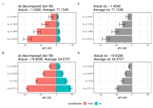
Figure 1: ShapleyBO results in iteration 59 of BO on $\Psi(\bm{\theta})=f(\bm{\theta})+\bm{\epsilon}$. Plots i and ii for $\lambda=1$ and plots iii and iv for $\lambda=10$, see (Croppi,, 2021, Fig. 5). Contributions ($phi$) are averaged over 30 proposals for each $\lambda$. On the right, the overall informativeness of the parameters is displayed ($cb$ contributions), and on the left the decomposition into $m$ (red) and $se$ (blue) contributions. Recall that cb is minimized. Error bars: Standard deviation of estimates.

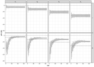
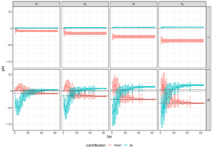
Figure 2: Informativeness paths for hyper ellipsoid optimization, see (Croppi,, 2021, Fig. 6). Plot on top displays $cb$ contributions with facets for parameters (vertical) and $\lambda$ (horizontal); beneath its decomposition into $m$ (red) and $se$ (blue) contributions. They are averaged over 30 proposals in each iteration and the uncertainty of the estimate is displayed with error bars using one standard deviation. The black dot-dashed line in the $\lambda=10$ plots displays the average contribution of the parameters in the $\lambda=1$ run.

Proposing new samples boils down to optimizing this confidence bound. To this end, let minimizing (w.l.o.g.) the confidence bound be a cooperative game along the lines of Section 2.2. It shall be defined as $(P,cb)$, or as two separate games $(P,m)$ and $(P,se)$, with $P$ being the grand coalition of Shapley values involved and $m$ and $se$ the mean and uncertainty prediction of the Shapley values, respectively. According to the linearity axiom the $cb$ contribution of any parameter $j$ of explicand $\tilde{\bm{\theta}}$ can then be decomposed into mean contribution $\phi_{j}(m)$ and uncertainty contribution $\phi_{j}(se)$.

$$\phi_{j}(cb)=\phi_{j}(m-\lambda se)=\phi_{j}(m)-\lambda\phi_{j}(se)$$ (5)

Thus, we can not only evaluate the overall informativeness of each parameter $\theta_{j}$, but also examine how both contributions $\phi(m)$ and $\phi(se)$ impact and drive the selection of proposed parameter values, shedding some light on the exploration-exploitation trade-off. On the background of recent work on uncertainty quantification McKeand et al., (2021); Hüllermeier and Waegeman, (2021); Psaros et al., (2023); Jansen et al., 2023b , we go beyond Croppi, (2021) and further aim at disentangling the uncertainty contribution $\phi_{j}(se)$ of a parameter $\theta_{j}$ into its epistemic (reducible) and aleatoric (irreducible) part. Aleaotoric uncertainty is typically caused by noise. The latter is particularly relevant in Bayesian optimization if it is of heteroscedastic nature, i.e., dependent on $\bm{\theta}$, since decision makers are often risk-averse. In other words, when deciding among two parameter configurations with equal mean target, most humans tend to opt for the one with lower variation. This motivates a risk-averse optimization problem: $\min_{\bm{\theta}\in\bm{\Theta}}f(\bm{\theta})-\alpha\cdot\epsilon(\bm{\theta})$ with $\epsilon(\bm{\theta})$ some noise that is non-constant in $\bm{\theta}$. Makarova et al., (2021) propose risk-averse heteroscedastic Bayesian optimization (RAHBO) which entails minimizing (w.l.o.g.) the risk-averse confidence bound (racb)

$$racb(\bm{\theta})=\widehat{\mu}(\bm{\theta})-\tau\cdot\widehat{\sigma}(\bm{\theta})+\alpha\cdot\widehat{\epsilon}(\bm{\theta}),$$ (6)

where $\widehat{\epsilon}(\bm{\theta})$ is an on-the-fly estimate of the noise. Due to $racb$’s additive structure, ShapleyBO can identify each parameter’s contribution to epistemic uncertainty reduction through $-\tau\cdot\widehat{\sigma}(\bm{\theta})$ and to aleatoric uncertainty avoidance through $\alpha\cdot\widehat{\epsilon}(\bm{\theta})$. By filtering out these exploratory contributions, the remainder of a parameter’s overall Shapley value can be identified as the parameter’s contribution to mean optimization through $\widehat{\mu}(\bm{\theta})$ (exploitation). We extend RAHBO by further dissecting the epistemic uncertainty into model uncertainty and approximation uncertainty. While the former describes uncertainty arising from model choise, the latter refers to classical statistical sampling uncertainty (Hüllermeier and Waegeman,, 2021, section 2.4). Notably, the model uncertainty asymptotically vanishes for GPs with universal approximation property, as the likelihood dominates the posterior in the limit, see Mangili, (2016). For the finite sample regime in BO, however, this asymptotic behavior is not relevant. In order to quantify model uncertainty, we rely on recently introduced prior-mean robust Bayesian optimization (PROBO) Rodemann, (2021); Rodemann and Augustin, (2021, 2022). PROBO avoids GP prior mean parameter misspecification by deploying imprecise Gaussian processes Mangili, (2016) as surrogate models. The rough idea of PROBO is to specify a set of prior mean values resulting in a set of posterior GPs. These latter give rise to an upper and lower mean estimate $\overline{\hat{\mu}}(\bm{\theta})_{c}$ and $\underline{\hat{\mu}}(\bm{\theta})_{c}$ subject to a degree of imprecision $c$. We define the uncertainty aware confidence bound (uacb) as follows: $uacb(\bm{\theta},\lambda,\rho,\alpha)=$

Since the remaining epistemic uncertainty is represented by the model’s $\widehat{\sigma}(\bm{\theta})$, we can interpret it as (an upper bound of) approximation uncertainty. Note that the uncertainty measured by PROBO is only a lower bound of the total model uncertainty, which also includes, for instance, uncertainty w.r.t. kernel parameter selection. The $uacb$ allows us to analyze as to what degree a parameter configuration is motivated by exploitation on the one hand or by reducing approximation, model or aleatoric uncertainty on the other hand. Since imprecise Gaussian processes are currently limited to univariate functions Mangili, (2016), we are not able to further attribute the contributions to multiple parameters. Future work will aim at multivariate extension. Nevertheless, the $uacb$ facilitates interpretation of proposals’ contributions to all these uncertainty types by means of ShapleyBO.

4 Illustrative Application

A deployment on synthetic functions allows us to validate our method, because we can formulate concrete expectations for the contributions based on the known functional form of the synthetic target function. We select a hyper-ellipsoid function, see Equation 8 below, where the parameters’ partial derivatives grow in $j$. Thus, we expect ShapleyBO to identify parameters with high $j$ to be most influential in BO.

Homoscedastic Target Function: Firstly, we illustrate ShapleyBO by optimizing $\Psi(\bm{\theta})=f(\bm{\theta})+\bm{\epsilon}$, where

$$f:[-5.12,5.12]^{4}\rightarrow\mathbb{R}_{0}^{+};\bm{\theta}\mapsto f(\mathbf{\bm{\theta}})=\sum_{j=1}^{4}j\cdot\mathbf{\theta}_{j}^{2}$$ (8)

with $j\in\{1,2,3,4\}$ and one unique optimum at $\bm{\theta}^{\ast}=(0,0,0,0)^{T}$ with $f(\bm{\theta}^{\ast})=0$. The noise $\epsilon$ is assumed be i.i.d. Gaussian and independent of $\bm{\theta}$ (homoscedastic). To control for the stochastic behavior of BO, $30$ optimizations with $60$ iterations each are run. After each optimization, ShapleyBO is applied. Results in each iteration are then averaged over all runs. Figure 1 has the results exemplarily for iteration 59. They are displayed for $\lambda=1$ (i and ii) and $\lambda=10$ (iii and iv). The analysis is based on (Croppi,, 2021, section 7.1)

As expected in light of the partial derivatives of $f(\bm{\theta})$, the contribution of $\theta_{j}$ grows with $j$. In contrast, uncertainty exhibits a diminutive and adverse effect. The uncertainty measurement $\hat{se}$ for the recommended setup falls below the mean $\bar{se}$, thus yielding a positive payout (negative contributions). Opting for a setup with an uncertainty estimate beneath the average is deemed a strategic compromise towards enhancing mean values at the expense of exploration. ShapleyBO facilitates a nuanced allocation of this trade-off across parameters, see both Figures 1 and 2. We will also study how the contributions change in the course of the optimization. Respective informativeness paths are shown in Figure 2. They reveal consistent patterns for $\lambda=1$, with a preference for higher parameters persisting across the board. Upon examining the lower plots’ decomposition, we see that both mean and uncertainty contributions remain constant over time. With a setting of $\lambda=10$, the algorithm conducts a thorough exploration of the parameter space, resulting in initially higher contributions and a more uniform informativeness among parameters. Over time, these contributions diminish smoothly, showing differences between parameters akin to the $\lambda=1$ scenario, but with a notable decrease in informativeness for higher parameters. Throughout the optimization process, the emphasis shifts from reducing uncertainty to prioritizing mean reduction, leading BO to favor configurations that perform well over those with high uncertainty. This transition is marked by a crossing in the contribution curves, see Figure 2, indicating a preference for mean reduction over uncertainty reduction, particularly for parameters with higher $\theta_{j}$, underscoring their importance for the optimization.

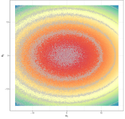
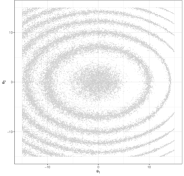
Figure 3: Contour plots of noisy ellipsoid function $\bm{\Psi}(\bm{\theta})=g(\bm{\theta})+\bm{\epsilon}(\bm{\theta})$, see Equations 9 and 10. Red: low $\bm{\Psi}(\bm{\theta})$; blue: high $\bm{\Psi}(\bm{\theta})$.

Heteroscedastic Target Function: Secondly, we illustrate ShapleyBO for Bayesian optimization of a two-dimensional ellipsoid function with noise depending on $\bm{\theta}$. That is, we minimize $\bm{\Psi}(\bm{\theta})=g(\bm{\theta})+\bm{\epsilon}(\bm{\theta})$, where

$$g\colon[-15,15]^{2}\to\mathbb{R}_{0}^{+};\;\bm{\theta}\mapsto f(\bm{\theta})=\sum_{i}^{2}i\cdot\theta_{i}^{2}$$ (9)

with $i\in\{1,2\}$ and

$$\bm{\epsilon}(\bm{\theta})=30\cdot\lvert\theta_{1}-15\rvert+0.3\cdot\lvert\theta_{2}-15\rvert.$$ (10)

That is, the noise grows strongly in $\theta_{1}$, but only moderately in $\theta_{2}$. Figure 3 shows contours of $g(\bm{\theta})$. It becomes evident that the function varies stronger w.r.t. $\theta_{2}$ than w.r.t. $\theta_{1}$, while the noise is strongly affected by $\theta_{1}$ and almost constant in $\theta_{2}$. Hence, we expect the respective Shapley values for aleatoric uncertainty contributions to be high for $\theta_{1}$ and low for $\theta_{2}$, and vice versa for exploitation (mean optimization). We run BO on $g(\bm{\theta})$ with risk-averse confidence bound ($racb$), see Equation 6; we again average over 30 restarts of BO with 60 iterations each. ShapleyBO delivers contributions for each $\theta_{j}$ to each of $racb$’s components in each of BO’s iterations. Table 1 has the results for exemplary iterations 1 and 2. Table 2 shows the contributions averaged over all $i\in\{1,\dots,60\}$ iterations and all $r\in\{1,\dots,30\}$ restarts. For instance, the averaged mean contributions of parameter $j$ are $\mkern 1.5mu\overline{\mkern-1.5mu\phi_{j}\mkern-1.5mu}\mkern 1.5mu(m)=\frac{1}{30}\sum_{r=1}^{30}\frac{1}{60}\sum_{i=1}^{60}\phi_{j,r,i}(m)$. It becomes evident that $\theta_{2}$ is more important for the mean minimization than $\theta_{1}$, while the latter contributes more to aleatoric uncertainty (noise) avoidance. The contributions to epistemic uncertainty reduction vary less with the parameters.

Summing up, the applications on both homo- and heteroscedastic target functions demonstrated that ShapleyBO manages to disentangle contributions of different parameters to different objectives of BO, thus providing valuable insights both into BO’s inner working (see Figures 1, 2 and Table 1) and about the target function itself (see Table 2).

iteration	$j$	$\phi_{j}(m)$	$\phi_{j}(se)$	$\phi_{j}(\hat{\epsilon})$	$\phi_{j}(racb)$
1	$\theta_{1}$	-100.2	2.4	-13.9	-111.8
1	$\theta_{2}$	-163.1	2.2	1.5	-159.4
2	$\theta_{1}$	-87.8	2.4	-37.7	-123.1
2	$\theta_{2}$	-165.6	1.6	3.3	-160.3

Table 1: Results of ShapleyBO for exemplary iterations $1$ and $2$ of BO with risk-averse confidence bound (Equation 6) on heteroscedastic target function $g(\bm{\theta})$ (Equation 10).

$j$	$\mkern 1.5mu\overline{\mkern-1.5mu\phi_{j}\mkern-1.5mu}\mkern 1.5mu(m)$	$\mkern 1.5mu\overline{\mkern-1.5mu\phi_{j}\mkern-1.5mu}\mkern 1.5mu(se)$	$\mkern 1.5mu\overline{\mkern-1.5mu\phi_{j}\mkern-1.5mu}\mkern 1.5mu(\hat{\epsilon})$
1	-48.48	4.20	-87.27
2	-157.73	6.88	0.24

Table 2: Results of ShapleyBO for averaged over all 60 iterations and all 30 BO restarts with risk-averse confidence bound (Equation 6) on heteroscedastic target function $g(\bm{\theta})$ (Equation 10).

5 Shapley-Assisted Human Machine Interface

The ability to interpret Bayesian optimization can be particularly useful for Human-In-the-Loop (HIL) applications, where users observe each step in the sequential optimization procedure. In this case ShapleyBO can inform users online, that is while the optimization is still running, about why certain actions were taken over others, instead of providing such explanations after the experiment has concluded. More specifically, we consider a human-AI collaborative framework Chakraborty et al., (2024); Gupta et al., (2023); Venkatesh et al., (2022); Akata et al., (2020); Borji and Itti, (2013), in which users can actively participate in the optimization by rejecting BO proposals and instead take actions on their own. As demonstrated in Section 4, Shapley values can provide structural insights on the relative importance of parameters for the optimization by filtering out uncertainty contributions, see $\mkern 1.5mu\overline{\mkern-1.5mu\phi_{j}\mkern-1.5mu}\mkern 1.5mu(m)$ in Table 2 for instance. Our general hypothesis is that basing the decision to intervene on this information will speed up the optimization. The underlying idea is that users can reject proposals in case the respective Shapley values do not align with the user’s knowledge about the optimization problem. To test this hypothesis, we benchmark a ShapleyBO-assisted human-AI team against teams without access to Shapley values. To better illustrate this, we consider the real-world use case of personalizing control parameters of a wearable, assistive back exosuit by Bayesian optimization.

5.1 Personalizing Soft Exosuits

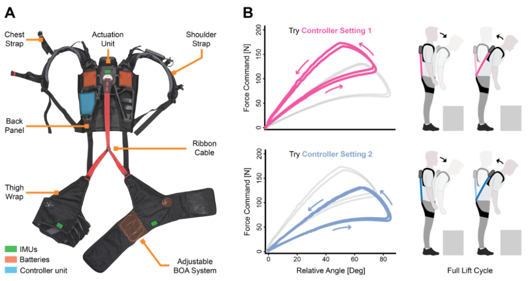
Figure 4: A: Assistive soft back exosuit. B: Force profile example for preference learning. Subjects are asked to compare controllers setting 1 (pink) to 2 (blue). Each option varies in the amount of lowering gain ($\theta_{low}$) and lifting gain ($\theta_{lif}$), see Arens et al., (2023).

Wearable robotic devices, such as exoskeletons and exosuits, have emerged as promising tools in mitigating risk of injury and aiding rehabilitation Siviy et al., (2023); Toxiri et al., (2019). With an increase in use cases and accessibility to a broader community, it has become apparent that the benefits of such devices can vary substantially between individuals. Besides design choices, which have to be made early on and are therefore often guided by (average) user anthropometrics, important factors influencing device efficacy are the magnitude and timing of assistance. To understand which settings work best for an individual, many studies follow HIL frameworks. These approaches comprise a feedback loop in which the impact of a controller modification on the objective function of interest is measured in real-time, and used to determine a set of control parameters that are likely improve upon the current optimum in the subsequent iteration. Given that under such conditions there is typically no known analytical relationship between control inputs and objective function outputs, sample efficient, query based methods like Bayesian Optimization have had considerable success for such applications Zhang et al., (2017); Ding et al., (2018).

5.2 Experimental Setup

Here, we explore the potential of ShapleyBO for the use-case of preference-based assistance optimization for a soft back exosuit, see Figure 4. To this end we consider a dataset in which 15 healthy individuals performed a simple, stoop lifting task with a light (2kg) external load Arens et al., (2023). Preference was queried in a forced-choice paradigm. That is, within each iteration, participants were consecutively exposed to two control parameter settings and asked to indicate which of the two options they preferred for completing the given task. Each of the settings comprised two parameters, referred to as lowering gain $\theta_{low}$ and lifting gain $\theta_{lif}$, which govern the amount of lowering and lifting assistance provided by the device, respectively, see also Figure 4. This preference feedback was used to compute a posterior utility distribution over the considered parameter domains, relying on a probit likelihood model and a GP prior over the latent user utility as described in Chu and Ghahramani, (2005). The experiment comprised three separate optimization blocks, in each of which the optimization was running for 12 iterations. To test ShapleyBO on this dataset, we averaged the three utility functions for each participant and interpolated by another GP to simulate the user’s ground truth utility function.

The remaining setup in our experimental study closely follows the one in Venkatesh et al., (2022). That is, the human can intervene in Bayesian optimization by rectifying proposals made by the algorithm, see pseudo code in Algorithm 1. We will compare our ShapleyBO-assisted human-BO team against the team in (Venkatesh et al.,, 2022, Algorithm 1) and three other baselines (human alone, BO alone, human-BO team with different intervention criterion). We model human decisions by another Bayesian optimization, following Borji and Itti, (2013); Venkatesh et al., (2022). This means that $\bm{\theta}^{human}=(\theta^{human}_{lif},\theta^{human}_{low})^{T}$ is found by optimizing an acquisition function modeling human preferences. We use a BO with the same surrogate model and acquisition function as for the outer loop, but with different exploration-exploitation preference and different initial design, representing differing risk-aversion and knowledge of the human, respectively.

Algorithm 1 Human-AI Collaborative BO

1:create an initial design $D=\{(\bm{\theta}^{(i)},\Psi^{(i)})\}_{i=1,...,n_{init}}$

2:while termination criterion is not fulfilled do

3:    train SM on data $D$

4:    propose $\bm{\theta}^{new}$ that optimizes $AF(SM(\bm{\theta}))$

5:    if intervention criterion is fulfilled then

6:         $\bm{\theta}^{new}\leftarrow\bm{\theta}^{human}$

7:    end if

8:    evaluate $\Psi$ on $\bm{\theta}^{new}$

9:    update $D\leftarrow D\cup{(\bm{\theta}^{new},\Psi(\bm{\theta}^{new}))}$

10:end while

11:return $\operatorname*{arg\,min}_{\bm{\theta}\in D}\Psi(\bm{\theta})$

Agent	A0	A1	A2	A3	A4
	BO	Human	Param-Team	Venkatesh et al., (2022)	Shap-Team
Intervention
Criterion	never	always	$\theta^{new}_{lif},\theta^{new}_{low}$	$k$-th iteration	$\phi_{lif}^{new}(m),\phi_{low}^{new}(m)$

Table 3: All agents: ShapleyBO-assisted A4 and baselines A0-A3.

All agents (A0, A1, A2, A3, A4) are equal to each other, the only difference being that the ShapleyBO-assisted agent intervenes based on Shapley values (A4), while the other agents intervene in each $k$-th iteration (A3) Venkatesh et al., (2022), based on the proposed parameters (A2), always (A1) or completely abstain from intervening (A0), see overview in Table 3. A4 has access to ShapleyBO and bases their decision to intervene (line 5 in Algorithm 1) on the alignment of the Shapley values of a BO proposal $\bm{\theta}^{new}=(\theta^{new}_{lif},\theta^{new}_{low})$ with the agent’s knowledge. More precisely, A4 accepts a BO proposal $\theta$ (does not intervene) if

$$\frac{1}{\beta}<\frac{\phi_{lif}^{new}(m)}{\phi_{low}^{new}(m)}/\frac{1}{T}\sum_{t=1}^{T}\frac{\phi_{lif}^{human}(m)_{t}}{\phi_{low}^{human}(m)_{t}}<\beta,$$ (11)

where $t\in\{1,\dots,T\}$ are iterations of the BO modeling the agent and $\phi(m)$ the Shapley mean contributions of $(\theta_{lif},\theta_{low})$, i.e., the exosuit’s lifting and lowering gain, respectively. We discuss different Shapley-based intervention criteria in the supplement. For A2’s intervention criterion we consider the alignment of $(\theta^{new}_{lif},\theta^{new}_{low})$ with the agents knowledge based on the parameter values itself. That is, A3 accepts a BO proposal (does not intervene) if

$$\frac{1}{\beta}<\frac{\theta^{new}_{lif}}{\theta^{new}_{low}}/\frac{1}{T}\sum_{t=1}^{T}\frac{\theta_{lif,t}^{human}}{\theta_{low,t}^{human}}<\beta.$$ (12)

5.3 Results

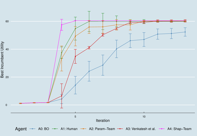
Figure 5: Results of Agents A0-A4 (see Table 3) in human-AI collaborative BO for simulated exosuit personalization (individual 1) with 10 iterations and 3 initial samples each. Error bars indicate $95\%$ confidence intervals; $k=2$ for A3, $\beta=2$ for A2 and A4.

We simulate 40 personalization rounds with 10 iterations and initial design of size 3 each for all five agents. We compare them with respect to optimization paths, which show best incumbent target values (utility) in a given iteration. The BO uses GP as AM and cb with $\lambda=20$ as AF; the BO modelling human proposals uses GP and cb with $\lambda=200$ and prior knowledge of $90$ data points.

Figure 5 exemplarily summarizes results for individual 1; results for remaining 14 individuals as well as experimental details can be found in the supplement. For all 15 subjects, ShapleyBO-assisted A4 (Shap-team) outperforms human and BO baseline as well as Venkatesh et al., (2022) and a team that bases their decision to intervene on the proposed parameters. This latter comparison particularly confirms that Shapley values are a meaningful measure for human-BO alignment that cannot be replaced by another notion of alignment without loss of efficiency. For 10 (among whom is subject 1, see Figure 5) out of 15 subjects the observed outperformance is significant at $95\%$ confidence level.

6 Discussion

By quantifying the contribution of each parameter to the proposals, ShapleyBO aids in the communication of the rationale behind specific optimization decisions. This interpretability is not only crucial for trust in HIL applications, it also enhances their efficiency. The use case of customizing exosuits illustrates the practical benefits of this approach, suggesting that ShapleyBO could be a valuable practical tool for personalizing soft back exosuits.

Our paper opens up a multitude of directions for future work. First and foremost, the simulation results in Section 5 based on real-world data motivate the actual deployment of Shapley-assisted human-in-the-loop optimization of exosuits in a user study. On the methodological end, extensions of ShapleyBO to multi-criteria BO appear straightforward, as long as additive acquisition functions are used. Moreover, a thorough mathematical study of the sublinear regret bounds of Bayesian optimization with confidence bound Srinivas et al., (2012) under Shapley-assisted human interventions might foster theoretical understanding of why Shapley-assisted teams outperform competitors.

Ethical Statement

The data used to estimate the utility functions was collected as part of another study Arens et al., (2023) for which ethical approval was obtained from the applicable institutional ethical review board. CJW is an inventor of at least one patent application describing the exosuit components described in the paper that have been filed with the U.S. Patent Office by Harvard University. Harvard University has entered into a licensing agreement with Verve Inc., in which CJW has an equity interest and a board position. The other authors declare that they have no competing interests.

Appendix A Supplement

A.1 Details on Experiments

Recall from the main paper that in our experimental setup, humans have the capability to modify the Bayesian optimization process by adjusting the algorithm’s suggestions, as illustrated in the pseudo-code below, which we print here again for ease of readability. We evaluate the performance of our ShapleyBO-enhanced human-BO collaboration against the approach described in (Venkatesh et al.,, 2022, Algorithm 1) and three other benchmark groups (solely human, solely BO, and a human-BO pair with an alternate intervention mechanism). The modeling of human decisions employs an additional layer of Bayesian optimization, inspired by Borji and Itti, (2013); Venkatesh et al., (2022), where $\bm{\theta}^{human}=(\theta^{human}_{lif},\theta^{human}_{low})^{T}$ is derived through an acquisition function that captures human preferences. This auxiliary BO uses the same surrogate and acquisition models as the primary loop but adjusts for human-specific risk tolerance and initial knowledge through different exploration-exploitation preference ($\lambda$ in $cb$) and initial designs, respectively. The specifications for both the original BO and the auxiliary BO modeling the human can be found below.

A.1.1 Model Specifications

The following non-exhaustive list summarizes the specifications for the conducted experiments.

• Bayesian Optimization

  • Surrogate Model: Gaussian Process

    • Kernel: Gaussian

      $$k(x,x^{\prime})\exp(-1/2\cdot(\lvert x-x^{\prime}\rvert/\theta)^{2}),$$

      where $\theta$ is the range parameter which was estimated from data (empirical Bayes)

    • Prior mean function estimated from data (empirical Bayes)

  • Acquisition Function: Confidence Bound

    • $\lambda_{bo}=20$

  • initial design size: $3$

• Human

  • Surrogate Model: Gaussian Process

    • Kernel: Gaussian

      $$k(x,x^{\prime})\exp(-1/2\cdot(\lvert x-x^{\prime}\rvert/\theta)^{2}),$$

      where $\theta$ is the range parameter which was estimated from data (empirical Bayes)

    • Prior mean function estimated from data (empirical Bayes)

  • Acquisition Function: Confidence Bound

    • $\lambda_{h}=200$

  • initial design size: $90$ (from a subset of the feature space, modeling prior knowledge of the human)

Algorithm 1 Human-AI Collaborative BO

1:create an initial design $D=\{(\bm{\theta}^{(i)},\Psi^{(i)})\}_{i=1,...,n_{init}}$

2:while termination criterion is not fulfilled do

3:    train SM on data $D$

4:    propose $\bm{\theta}^{new}$ that optimizes $AF(SM(\bm{\theta}))$

5:    if intervention criterion is fulfilled then

6:         $\bm{\theta}^{new}\leftarrow\bm{\theta}^{human}$

7:    end if

8:    evaluate $\Psi$ on $\bm{\theta}^{new}$

9:    update $D\leftarrow D\cup{(\bm{\theta}^{new},\Psi(\bm{\theta}^{new}))}$

10:end while

11:return $\operatorname*{arg\,min}_{\bm{\theta}\in D}\Psi(\bm{\theta})$

Agent	A0	A1	A2	A3	A4
	BO	Human	Param-Team	Venkatesh et al., (2022)	Shap-Team
Intervention
Criterion	never	always	$\theta^{new}_{lif},\theta^{new}_{low}$	$k$-th iteration	$\phi_{lif}^{new}(m),\phi_{low}^{new}(m)$

Table 4: All agents: ShapleyBO-assisted A4 and baselines A0-A3.

Varying both $\lambda_{h}$ and $\lambda_{bo}$ did not affect the overall results significantly. Drastically decreasing initial design size for the human led to all human-BO teams (A2, A3, A4) to be outperformed by the the BO Baseline A0. We reason that a certain advantage in knowledge by the humans is key to successful human-BO collaboration.

A.1.2 Details on Simulations

We computed 40 repetitions of the described procedure on a Linux High-performance cluster. The experiments were tested with R versions 4.3.2, 4.2.0, 4.1.6, and 4.0.3 on Linux Ubuntu 20.04, Linux Debian 10, and Windows 11 Pro Build 22H2. Further details as well as documentation of how to reproduce the results can be found in the readme-file of the anonymous repository:

https://anonymous.4open.science/r/ShapleyBO-E65D

A.1.3 Alternative Intervention Criteria

We varied $\beta$ for both A2 and A4 and did not observe significant changes in the results. Moreover, we considered different intervention criteria based on previous experience of the human rather than hard coded like Equations 11 and 12 in the main paper. The idea was to learn the criterion from previous BO runs. The so acquired data (proposals $\bm{\theta}$ and respective Shapley values as well as the evaluated target $\Psi(\bm{\theta})$) was used to train an ML model to represent the learned knowledge in previous BO iteration. To this end, we rely on classification and regression trees (CART), as they are easy to interpret, flexible and robust Loh, (2014); Fernández-Delgado et al., (2014); Nalenz et al., (2024). We particularly rely on their ability to learn logical rules that can then be used as intervention criteria. The pruned version of a tree delivers a decision rule of required complexity, see Figure 6. It represents the human’s knowledge about the relationship between the proposals’ Shapley values and the obtained target values.

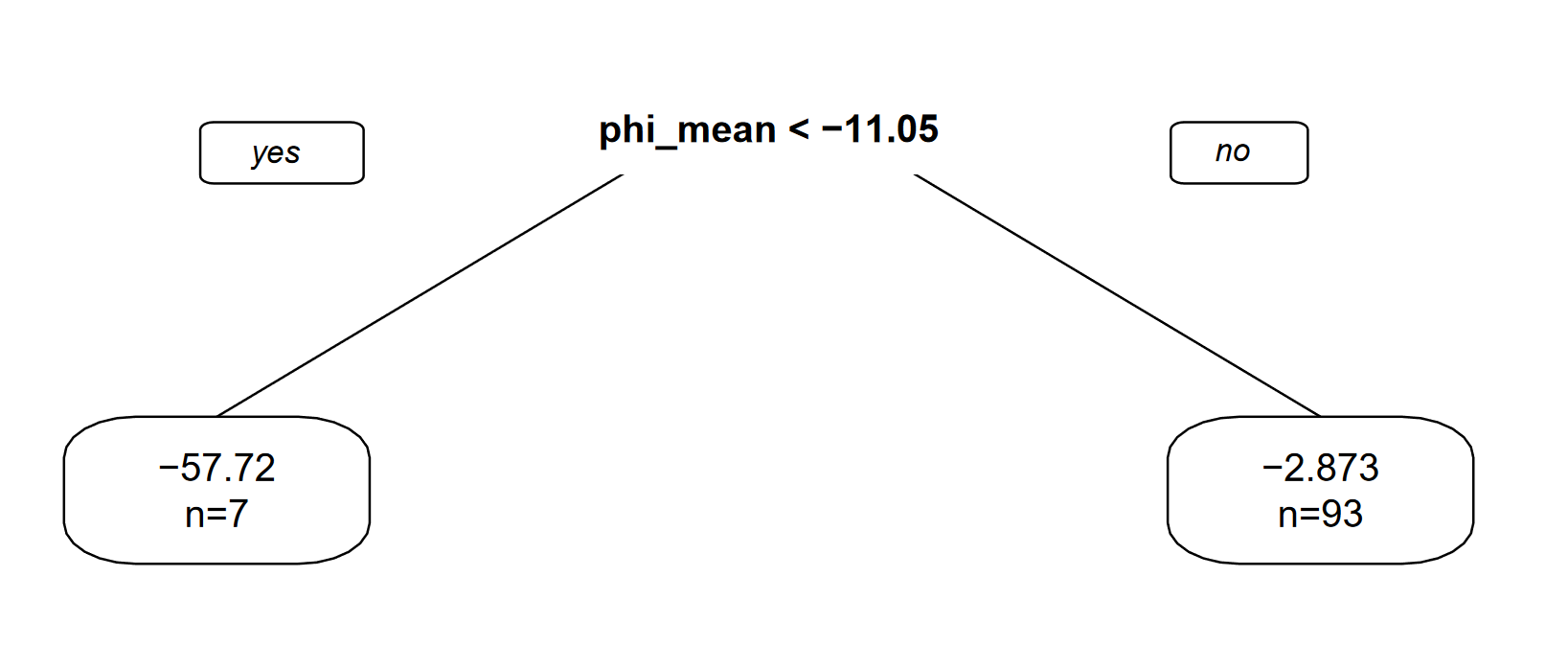
Figure 6: Regression tree learned from Shapley-assisted BO. It predicts a target value of $\Psi(\bm{\theta})=-57.72$ for BO proposals where $\theta_{lif}$ (lifting gain) has a Shapley contribution to the mean component of cb lower than $-11.05$, i.e., $\phi_{lif}(m)<-11.05$. Using this learned rule as an intervention criterion in human-AI collaborative BO translates to rejecting the automatically generated BO proposals and rectifying them by human’s proposals in case their respective Shapley values fulfill $\phi_{lif}(m)<-11.05$.

Replacing the hard-coded intervention criteria (Equation 11 and 12 in the main paper) by those learned through a regression tree did not change the results significantly, see Figure 7 and Figure 8. We ran the same experiments as described in the main paper, but additionally included a Shapley-assisted human-BO team with intervention criterion learned through regression trees (yellow).

As becomes evident, the reported results are relatively robust with regard to the concrete specification of the intervention criterion. That is, the precise nature of the criterion (see also discussion of results for altered $\beta$) and whether it is hard-coded or learned from previous BO iterations does not alter the results significantly.

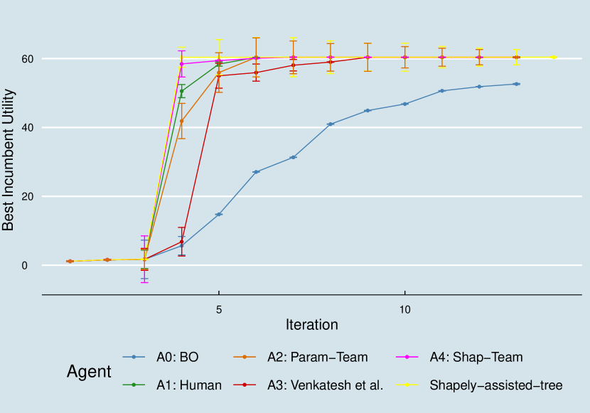
Figure 7: Results of Agents A0-A4 (see Table 4) and additional agent with tree-based intervention criterion in human-AI collaborative BO for simulated exosuit personalization (individual 1) with 10 iterations and 3 initial samples each. Error bars indicate $95\%$ confidence intervals; $k=2$ for A3, $\beta=2$ for A2 and A4.

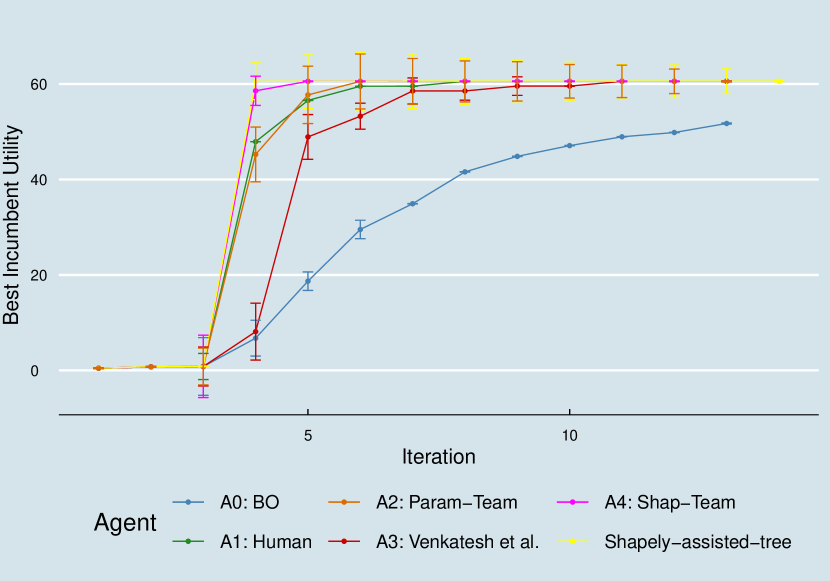
Figure 8: Results of Agents A0-A4 (see Table 4) and additional agent with tree-based intervention criterion in human-AI collaborative BO for simulated exosuit personalization (randomly selected individual) with 10 iterations and 3 initial samples each. Error bars indicate $95\%$ confidence intervals; $k=2$ for A3, $\beta=2$ for A2 and A4.

A.1.4 Research Hypotheses

Experimental design was motivated by the following hypotheses that were formulated beforehand.

Hypothesis 1 (BO Baseline).

Human-BO teams are more efficient than BO alone.

Hypothesis 2 (Human Baseline).

Human-BO teams are more efficient than a human without access to BO.

Hypothesis 3 (Venkatesh et al., (2022) Baseline).

An agent in human-AI collaborative BO that intervenes based on Shapley values is more efficient than an agent who does intervene in each $k$-th iteration.

Hypothesis 4 (Parameter-informed Baseline).

An agent in human-AI collaborative BO that intervenes based on Shapley values is more efficient than an agent who intervenes based on the discrepancy between the proposed parameter values.

Efficiency in Hypotheses 1 through 4 refers to the cumulative regret (distances to optimum summed over all iterations). Hypotheses 1 and 2 make sure Shapley-assisted human-BO teams do not simply outperform competitors due to the fact that the human is uniformly superior to BO, or vice versa. Notably, hypotheses 1 through 4 were treated as scientific research hypotheses rather than statistical hypotheses. We leave a rigorous statistical benchmarking analysis along the lines of Demšar, (2006); Jansen et al., 2023a to future work as well as multi-criteria comparison Jansen et al., 2023b ; Blocher et al., (2023); Rodemann and Blocher, (2024) of the optimization agents.

A.2 Additional Experiments and Future Work

As already hinted at in the subsections on model specifications and alternative intervention criteria in Section A.1.3, we did conduct some robustness analysis. The results from varying the intervention criteria can be see in Figures 7 and 8 and have been discussed above. In what follows, we exemplarily showcase some results from experiments where we altered $\lambda_{h}$ and $\lambda_{BO}$. Figure 9 has the results for $\lambda_{h}=\lambda_{bo}=40$, i.e. a more balanced exploration-exploitation preference between human and BO. The results are hardly affected by the more balanced exploration-exploitation scheme.

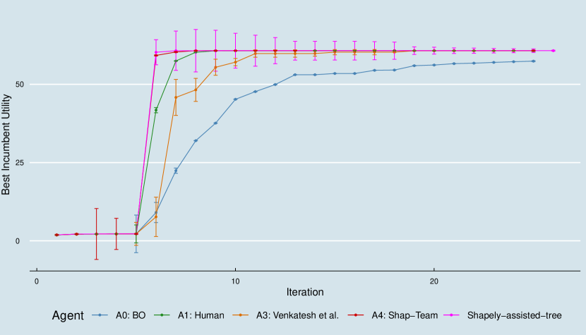
Figure 9: Results of for simulated exosuit personalization (randomly selected individual) for $\lambda_{h}=\lambda_{bo}=40$ with 20 iterations and 5 initial samples each. Error bars indicate $95\%$ confidence intervals.

Besides the above presented additional experiments for exosuit personalization, we also tested ShapleyBO in a univariate scenario, where deployment of the uncertainty-aware confidence bound (Equation 7 in main paper) was possible. We focused on the concrete case of minimizing metabolic cost by step size adaption of powered prosthetics for walking assistance Kim et al., (2017). The publicly available data contains measurements on 9 patients. We use each of them to fit a surrogate function that we optimize by BO. The proposal are interpreted by Shapley values, showcasing the potential use of disentangling the uncertainty contributions even in a univariate setup.

A.3 Computational details

A principal hurdle in applying Shapley values (SVs) within the realm of interpretable machine learning (IML) is their computational intensity. To precisely calculate Shapley values, one must evaluate the model across all conceivable feature subsets. Such exact calculations are known to possess exponential time complexity Štrumbelj and Kononenko, (2014), making the use of approximation methods such as Monte Carlo (MC) sampling a practical necessity.

For instance, Merrick and Taly, (2019) devised the Explanation Game, an innovative sampling approach that employs importance sampling to enhance the accuracy of Shapley value estimates.Ignatov and Kwuida, (2022) introduced a method rooted in formal concept analysis for assessing Shapley values over finite attribute sets, while Luther et al., (2023) applied causal structure learning to pinpoint feature independencies, thereby streamlining Shapley value computation.

In our work, we adopt a traditional MC sampling strategy, supplemented by a novel algorithm from Croppi, (2021), designed to accurately determine an adequate sample size for Shapley value estimation in Bayesian optimization contexts. This algorithm presents a viable means of identifying the requisite sample volume for efficient SV computation. Let us define the payout function

$$\mathcal{P}(v)=\hat{f}^{v}(\tilde{\bm{\theta}})-\frac{1}{n}\sum_{i}\hat{f}^{v}(\bm{\theta}^{(i)}),$$ (13)

intended for distribution among the explicand’s parameters $\tilde{\bm{\theta}}$, where $\hat{f}^{v}$ predicts outcomes $v=\{cb,m,se\}$ and $\{\bm{\theta}^{(i)}\}_{i=1}^{n}$ denotes a series of instances. As per the efficiency axiom, the equality $\sum_{j}\phi_{j}(v)=\mathcal{P}(v)$ is expected. However, due to approximation in calculating true contributions, this process incurs an efficiency error, represented as

$$\Delta_{eff}^{K}(v)=\sum_{j}\hat{\phi}_{j}^{K}(v)-\mathcal{P}(v),$$ (14)

with $K$ symbolizing the MC sample count. The discrepancy $\Delta_{eff}^{K}(v)$ diminishes as $K$ increases, aligning with the asymptotic distribution of $\hat{\phi}_{j}(v)$. An error greater (lesser) than zero indicates an overallocation (underallocation) of payout, necessitating an adjustment in contributions. While the precise contributions requiring adjustment remain uncertain, redistributing $\Delta_{eff}^{K}(v)$ entirely to a single parameter would arguably be the least equitable.

Our focus lies not on rectifying the outcomes but on evaluating the adequacy of $K$. For computational simplicity, we redefine $\Delta_{eff}^{K}(v)$ as $|\sum_{j}\hat{\phi}_{j}^{K}(v)-\mathcal{P}(v)|$. Moreover, we introduce

$$\delta^{K}(v)=min\{\bm{d_{1}}(\hat{\phi}_{j}^{K}(v),\hat{\phi}_{l}^{K}(v))_{j\neq l}\},$$ (15)

the minimal $L_{1}$ distance between any two distinct parameter Shapley values. A sample size $K$ is deemed sufficient if $\Delta_{eff}^{K}(v)<\delta^{K}(v)$, ensuring that adjustments for efficiency error do not alter the importance rankings. If this condition is not met, $K$ must be increased.

A sufficient sample size is thus determined through a greedy forward search. Below, a visual representation of this methodology is provided, and Algorithm 4 concisely outlines the primary procedural steps, see also the respetive pseudo-code in the following section.

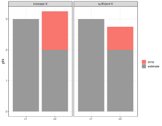
Figure 10: Example of the idea behind checkSampleSize, see (Croppi,, 2021, Figure 16). Estimated Shapley values of two features named $x_{1}$ and $x_{2}$ in grey give threshold $\delta^{K}=3-2=1$. The efficiency error in red varies for different $K$. Suppose $\Delta_{eff}^{K}(v)<0$. The error is thus added entirely to $x_{2}$. In the left plot the sample size $K$ is not sufficient because redistributing the resulting error would make $x_{2}$ more important than $x_{1}$. Instead, in the right plot $K$ would be sufficient. In case of $\Delta_{eff}^{K}(v)>0$ removing the error completely from $x_{1}$ would lead to the same conclusion for $K$.

A.4 Pseudo-Code

In what follows, we summarize the main algorithmic procedures in pseudo-code: The general estimation of the Shapley values, the main procedure to retrieve Shapley values from any iteration in Bayesian Optimization, and the above mentioned procedure to check the sample size required for MC-estimation of the Shapley values. Detailed implementation of all procedures in R R Core Team, (2020) (dependencies: mlrMBO Bischl et al., (2017), iml Molnar et al., (2018)) can be accessed in folder R of:

https://anonymous.4open.science/r/ShapleyBO-E65D

Algorithm 2 Estimation of the Shapley values

1:explicand $\tilde{\bm{\theta}}$, feature index $j$, model $\hat{f}$ and sample size $K$

2:for $k=1\to K$ do

3:     sample (with replacement) an instance $\bm{z}\in\bm{\Theta}$

4:     sample (with replacement) an order $\pi\in\Pi(P)$

5:     order $\tilde{\bm{\theta}}$ and $\bm{z}$ according to $\pi$

6:          $\tilde{\bm{\theta}}_{\pi}=(\tilde{\theta}_{(1)},\ldots,\tilde{\theta}_{(p)})$

7:          $\bm{z}_{\pi}=(z_{(1)},\ldots,z_{(p)})$

8:     construct two new instances

9:          $\tilde{\bm{\theta}}_{+j}=(\tilde{\theta}_{(1)},\ldots,\tilde{\theta}_{(j-1)},\tilde{\theta}_{(j)},z_{(j+1)},\ldots,z_{(p)})$

10:          $\tilde{\bm{\theta}}_{-j}=(\tilde{\theta}_{(1)},\ldots,\tilde{\theta}_{(j-1)},z_{(j)},z_{(j+1)},\ldots,z_{(p)})$

11:     $\hat{\phi}_{j}^{k}(v)=\hat{f}(\tilde{\bm{\theta}}_{+j})-\hat{f}(\tilde{\bm{\theta}}_{-j})$

12:end for

13:$\hat{\phi}_{j}(v)=\frac{1}{K}\sum_{k=1}^{K}\hat{\phi}_{j}^{k}(v)$

Algorithm 3 ShapleyBO

1:BO result object bo, iteration of interest $t$, sample size $K$

2:get explicand from bo: $\tilde{\bm{\theta}}=\bm{\theta}^{new}_{t}$

3:sample $1000\cdot p$ points $\bm{Z}$ from $\bm{\Theta}$ to approximate the space

4:compute $\hat{\bm{\phi}}(m)=(\hat{\phi}_{1}(m),\ldots,\hat{\phi}_{p}(m))$:

5:      get SM from bo: $\hat{f}_{m}=\hat{f}_{t}^{mean}$

6:      explain $\tilde{\bm{\theta}}$ with Shapley() using $\bm{Z}$, $\hat{f}_{m}$ and $K$

7:compute $\hat{\bm{\phi}}(se)=(\hat{\phi}_{1}(se),\ldots,\hat{\phi}_{p}(se))$:

8:      get SM from bo: $\hat{f}_{se}=\hat{f}_{t}^{uncertainty}$

9:      explain $\tilde{\bm{\theta}}$ with Shapley() using $\bm{Z}$, $\hat{f}_{se}$ and $K$

10:compute $\hat{\bm{\phi}}(cb)$ with linearity axiom: $\hat{\bm{\phi}}(cb)=\hat{\bm{\phi}}(m)-\lambda\hat{\bm{\phi}}(se)$

Algorithm 4 checkSampleSize

1:ShapleyBO results for $\tilde{\bm{\theta}}_{t}$ with size $K$, models $\hat{f}^{v}$ with $v=\{cb,m,se\}$

2:for $w$ in $v$ do

3:     compute payout $\mathcal{P}(w)$, error $\Delta_{eff}^{K}(w)$  and threshold $\delta^{K}(w)$

4:     if $\Delta_{eff}^{K}(w)<\delta^{K}(w)$ then

5:         $K_{w}$ = T

6:     end if

7:     if $\Delta_{eff}^{K}(w)\geq\delta^{K}(w)$ then

8:         $K_{w}$ = F

9:     end if

10:end for

11:if $(K_{cb},K_{m},K_{se})=(\texttt{T},\texttt{T},\texttt{T})$ then

12:     $K$ is high enough

13:else if $(K_{cb},K_{m},K_{se})\neq(\texttt{T},\texttt{T},\texttt{T})$ then

14:     $K$ should be increased

15:end if

A.5 Additional Results

For ease of exposition, we only included detailed results for individual 1 in the main paper. Results for remaining 14 individuals are displayed by Figures 11 through 24 in what follows. As stated in the main paper, ShapleyBO-assisted human-BO teams outperform competitors on average for all individuals. For 10 out 15 individuals, this finding is significant at confidence level of $95\%$

Individual 2:

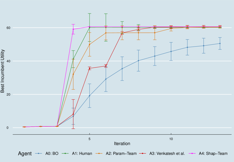
Figure 11: Results of Agents A0-A4 (see Table 4) in human-AI collaborative BO for simulated exosuit personalization (individual 2) with 10 iterations and 3 initial samples each. Error bars indicate $95\%$ confidence intervals; $k=2$ for A3, $\beta=2$ for A2 and A4.

Individual 3:

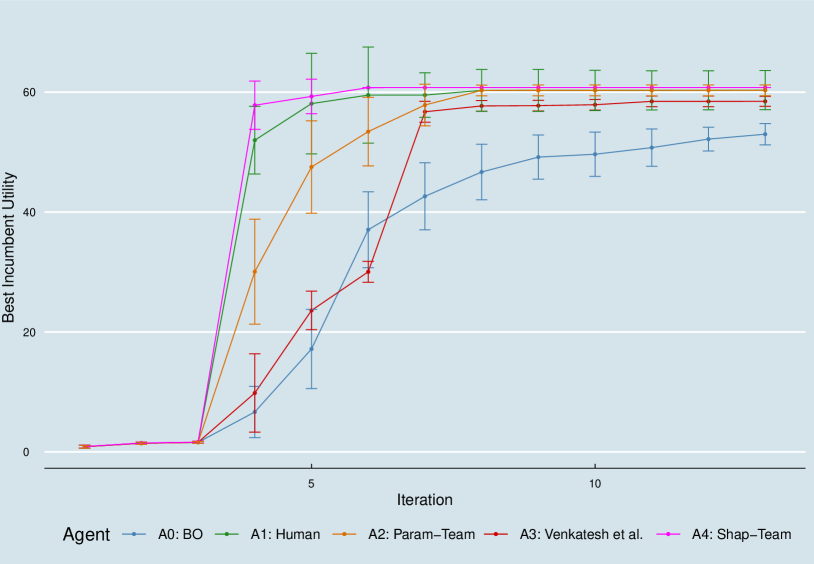
Figure 12: Results of Agents A0-A4 (see Table 4) in human-AI collaborative BO for simulated exosuit personalization (individual 3) with 10 iterations and 3 initial samples each. Error bars indicate $95\%$ confidence intervals; $k=2$ for A3, $\beta=2$ for A2 and A4.

Individual 4:

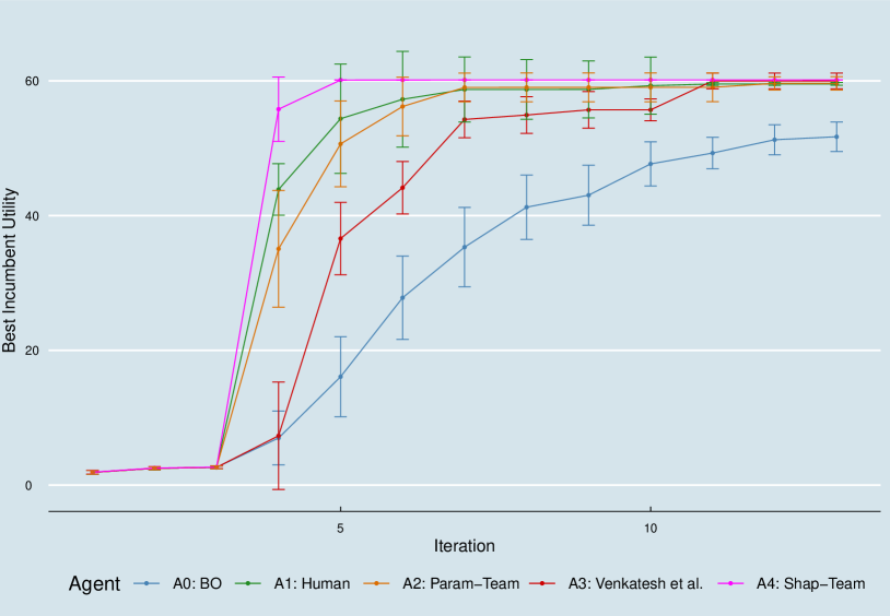
Figure 13: Results of Agents A0-A4 (see Table 4) in human-AI collaborative BO for simulated exosuit personalization (individual 4) with 10 iterations and 3 initial samples each. Error bars indicate $95\%$ confidence intervals; $k=2$ for A3, $\beta=2$ for A2 and A4.

Individual 5:

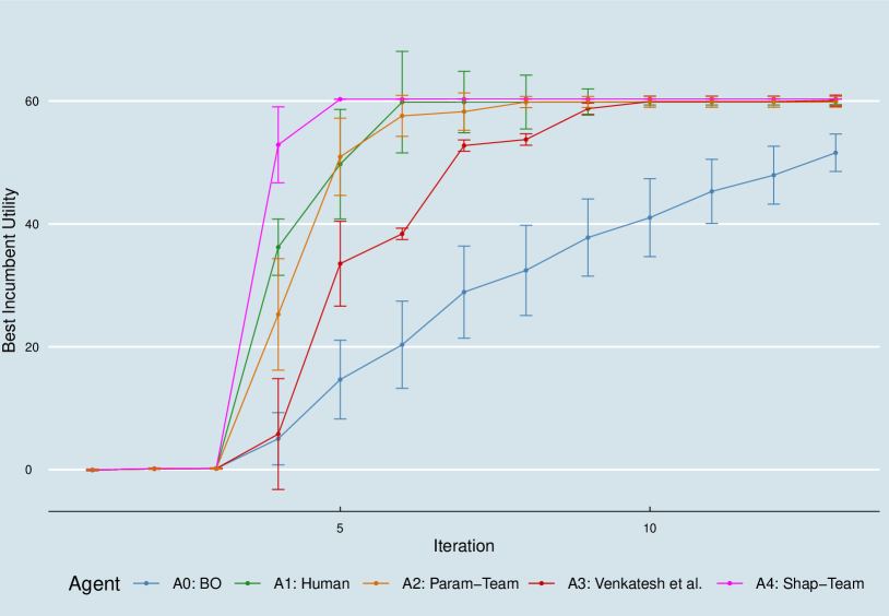
Figure 14: Results of Agents A0-A4 (see Table 4) in human-AI collaborative BO for simulated exosuit personalization (individual 5) with 10 iterations and 3 initial samples each. Error bars indicate $95\%$ confidence intervals; $k=2$ for A3, $\beta=2$ for A2 and A4.

Individual 6:

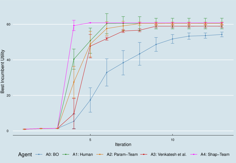
Figure 15: Results of Agents A0-A4 (see Table 4) in human-AI collaborative BO for simulated exosuit personalization (individual 6) with 10 iterations and 3 initial samples each. Error bars indicate $95\%$ confidence intervals; $k=2$ for A3, $\beta=2$ for A2 and A4.

Individual 7:

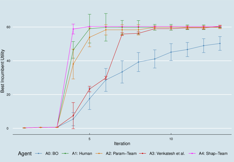
Figure 16: Results of Agents A0-A4 (see Table 4) in human-AI collaborative BO for simulated exosuit personalization (individual 7) with 10 iterations and 3 initial samples each. Error bars indicate $95\%$ confidence intervals; $k=2$ for A3, $\beta=2$ for A2 and A4.

Individual 8:

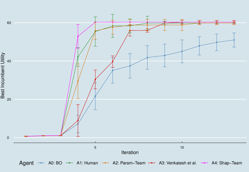
Figure 17: Results of Agents A0-A4 (see Table 4) in human-AI collaborative BO for simulated exosuit personalization (individual 8) with 10 iterations and 3 initial samples each. Error bars indicate $95\%$ confidence intervals; $k=2$ for A3, $\beta=2$ for A2 and A4.

Individual 9:

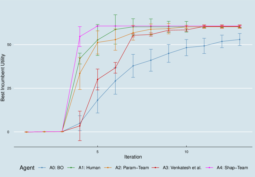
Figure 18: Results of Agents A0-A4 (see Table 4) in human-AI collaborative BO for simulated exosuit personalization (individual 9) with 10 iterations and 3 initial samples each. Error bars indicate $95\%$ confidence intervals; $k=2$ for A3, $\beta=2$ for A2 and A4.

Individual 10:

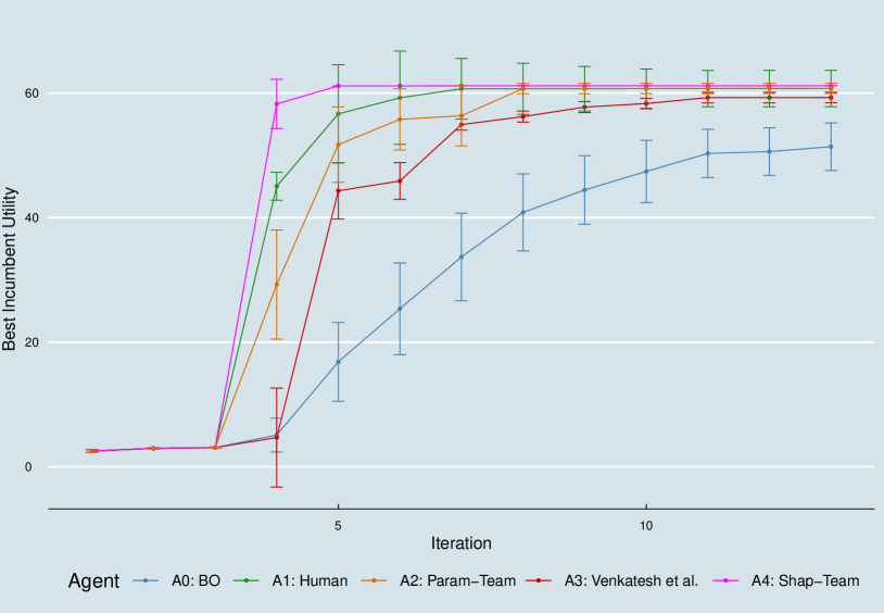
Figure 19: Results of Agents A0-A4 (see Table 4) in human-AI collaborative BO for simulated exosuit personalization (individual 10) with 10 iterations and 3 initial samples each. Error bars indicate $95\%$ confidence intervals; $k=2$ for A3, $\beta=2$ for A2 and A4.

Individual 11:

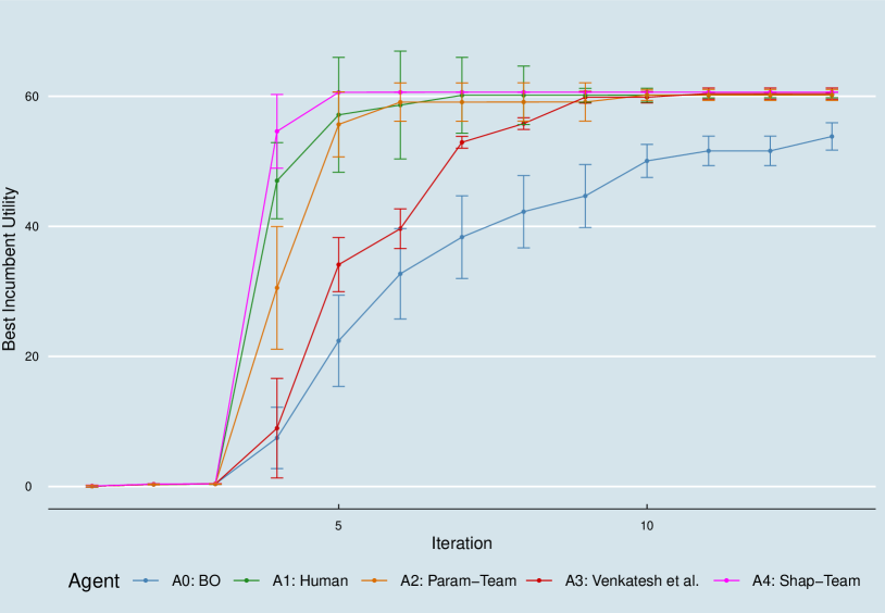
Figure 20: Results of Agents A0-A4 (see Table 4) in human-AI collaborative BO for simulated exosuit personalization (individual 11) with 10 iterations and 3 initial samples each. Error bars indicate $95\%$ confidence intervals; $k=2$ for A3, $\beta=2$ for A2 and A4.

Individual 12:

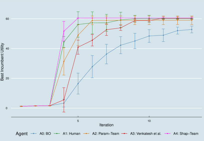
Figure 21: Results of Agents A0-A4 (see Table 4) in human-AI collaborative BO for simulated exosuit personalization (individual 12) with 10 iterations and 3 initial samples each. Error bars indicate $95\%$ confidence intervals; $k=2$ for A3, $\beta=2$ for A2 and A4.

Individual 13:

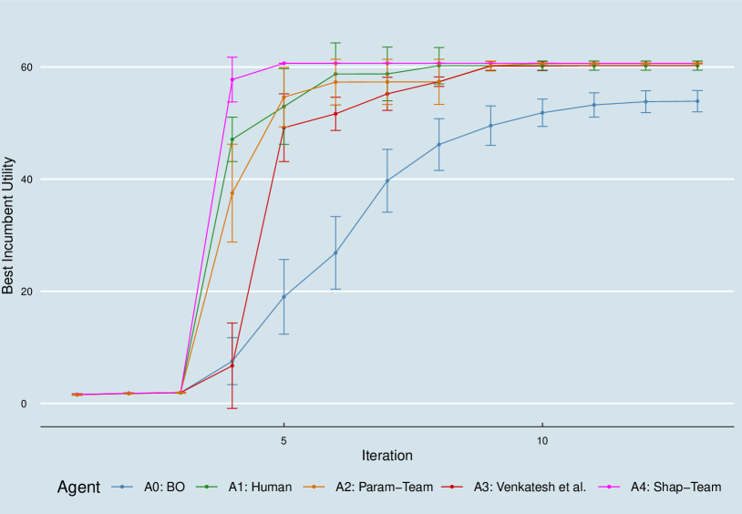
Figure 22: Results of Agents A0-A4 (see Table 4) in human-AI collaborative BO for simulated exosuit personalization (individual 13) with 10 iterations and 3 initial samples each. Error bars indicate $95\%$ confidence intervals; $k=2$ for A3, $\beta=2$ for A2 and A4.

Individual 14:

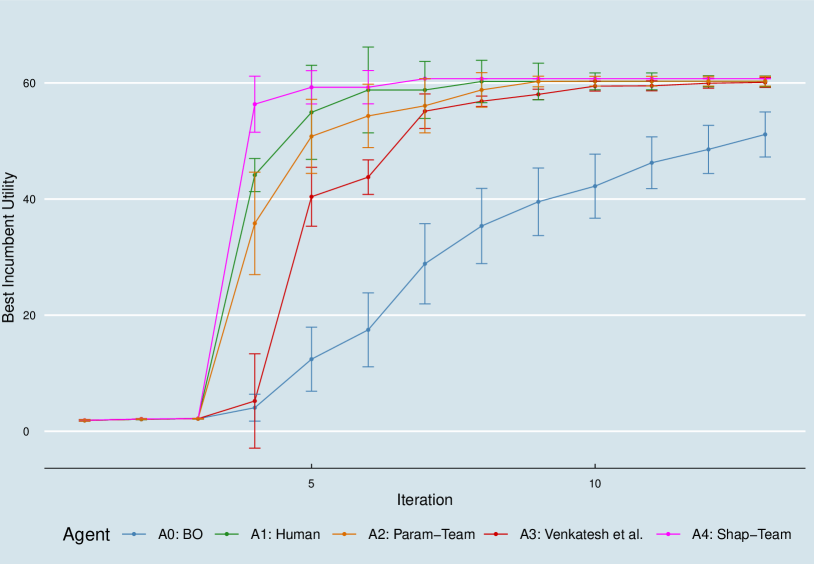
Figure 23: Results of Agents A0-A4 (see Table 4) in human-AI collaborative BO for simulated exosuit personalization (individual 14) with 10 iterations and 3 initial samples each. Error bars indicate $95\%$ confidence intervals; $k=2$ for A3, $\beta=2$ for A2 and A4.

Individual 15:

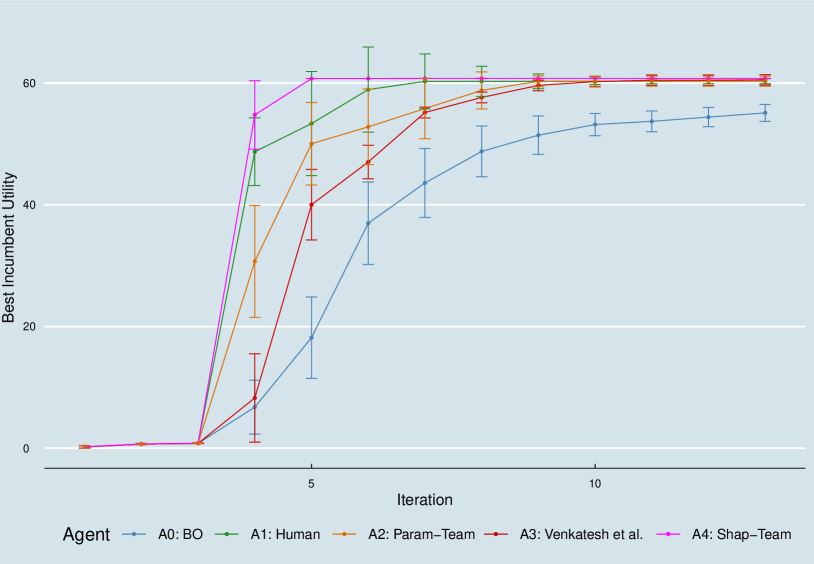
Figure 24: Results of Agents A0-A4 (see Table 4) in human-AI collaborative BO for simulated exosuit personalization (individual 15) with 10 iterations and 3 initial samples each. Error bars indicate $95\%$ confidence intervals; $k=2$ for A3, $\beta=2$ for A2 and A4.

References

- Aas et al., (2021) Aas, K., Jullum, M., and Løland, A. (2021). Explaining individual predictions when features are dependent: More accurate approximations to shapley values. Artificial Intelligence, 298:103502.
- Adachi et al., (2024) Adachi, M., Planden, B., Howey, D. A., Maundet, K., Osborne, M. A., and Chau, S. L. (2024). Looping in the human: Collaborative and explainable bayesian optimization. In 27th International Conference on Artificial Intelligence and Statistics (AISTATS), volume 238. PMLR.
- Akata et al., (2020) Akata, Z., Balliet, D., de Rijke, M., Dignum, F., Dignum, V., Eiben, G., Fokkens, A., Grossi, D., Hindriks, K., Hoos, H., Hung, H., Jonker, C., Monz, C., Neerincx, M., Oliehoek, F., Prakken, H., Schlobach, S., van der Gaag, L., van Harmelen, F., van Hoof, H., van Riemsdijk, B., van Wynsberghe, A., Verbrugge, R., Verheij, B., Vossen, P., and Welling, M. (2020). A research agenda for hybrid intelligence: Augmenting human intellect with collaborative, adaptive, responsible, and explainable artificial intelligence. Computer, 53(8):18–28.
- Arens et al., (2023) Arens, P., Quirk, D. A., Pan, W., Yacoby, Y., Doshi-Velez, F., and Walsh, C. J. (2023). Preference-based assistance optimization for lifting and lowering with a soft back exosuit. Submitted for publication. Manuscript in review as of December 2023.
- Auer et al., (2002) Auer, P., Cesa-Bianchi, N., and Fischer, P. (2002). Finite-time analysis of the multiarmed bandit problem. Machine Learning, 47:235–256.
- AV et al., (2024) AV, A. K., Shilton, A., Gupta, S., Rana, S., Greenhill, S., and Venkatesh, S. (2024). Enhanced bayesian optimization via preferential modeling of abstract properties. arXiv preprint arXiv:2402.17343.
- Bakshi et al., (2023) Bakshi, S., Sharma, S., and Khanna, R. (2023). Shapley-value-based hybrid metaheuristic multi-objective optimization for energy efficiency in an energy-harvesting cognitive radio network. Mathematics, 11(7):1656.
- Beechey et al., (2023) Beechey, D., Smith, T. M. S., and Şimşek, O. (2023). Explaining reinforcement learning with shapley values. In Krause, A., Brunskill, E., Cho, K., Engelhardt, B., Sabato, S., and Scarlett, J., editors, Proceedings of the 40th International Conference on Machine Learning, volume 202 of Proceedings of Machine Learning Research, pages 2003–2014. PMLR.
- Bischl et al., (2017) Bischl, B., Richter, J., Bossek, J., Horn, D., Thomas, J., and Lang, M. (2017). mlrmbo: A modular framework for model-based optimization of expensive black-box functions. arXiv preprint arXiv:1703.03373.
- Blocher et al., (2023) Blocher, H., Schollmeyer, G., Jansen, C., and Nalenz, M. (2023). Depth functions for partial orders with a descriptive analysis of machine learning algorithms. In Miranda, E., Montes, I., Quaeghebeur, E., and Vantaggi, B., editors, Proceedings of the Thirteenth International Symposium on Imprecise Probability: Theories and Applications, volume 215 of Proceedings of Machine Learning Research, pages 59–71. PMLR.
- Borji and Itti, (2013) Borji, A. and Itti, L. (2013). Bayesian optimization explains human active search. Advances in Neural Information Processing Systems, 26.
- Breiman, (2001) Breiman, L. (2001). Random forests. Machine Learning, 45(1):5–32.
- Burton et al., (2023) Burton, J. W., Stein, M.-K., and Jensen, T. B. (2023). Beyond algorithm aversion in human-machine decision-making. In Judgment in Predictive Analytics, pages 3–26. Springer.
- Chakraborty et al., (2024) Chakraborty, T., Seifert, C., and Wirth, C. (2024). Explainable bayesian optimization. arXiv preprint arXiv:2401.13334.
- Chakraborty et al., (2023) Chakraborty, T., Wirth, C., and Seifert, C. (2023). Post-hoc rule based explanations for black box bayesian optimization. In European Conference on Artificial Intelligence, pages 320–337. Springer.
- Chu and Ghahramani, (2005) Chu, W. and Ghahramani, Z. (2005). Preference learning with gaussian processes. In Proceedings of the 22nd International Conference on Machine Learning, pages 137–144.
- Cisse et al., (2023) Cisse, A., Evangelopoulos, X., Carruthers, S., Gusev, V. V., and Cooper, A. I. (2023). Hypbo: Expert-guided chemist-in-the-loop bayesian search for new materials. arXiv preprint arXiv:2308.11787.
- Croppi, (2021) Croppi, F. (2021). Explaining sequential model-based optimization. Master Thesis, LMU Munich.
- Demšar, (2006) Demšar, J. (2006). Statistical comparisons of classifiers over multiple data sets. The Journal of Machine learning research, 7:1–30.
- Dietvorst et al., (2015) Dietvorst, B. J., Simmons, J. P., and Massey, C. (2015). Algorithm aversion: people erroneously avoid algorithms after seeing them err. Journal of Experimental Psychology: General, 144(1):114.
- Ding et al., (2018) Ding, Y., Kim, M., Kuindersma, S., and Walsh, C. J. (2018). Human-in-the-loop optimization of hip assistance with a soft exosuit during walking. Science Robotics, 3(15):eaar5438.
- Fernández-Delgado et al., (2014) Fernández-Delgado, M., Cernadas, E., Barro, S., and Amorim, D. (2014). Do we need hundreds of classifiers to solve real world classification problems? The journal of machine learning research, 15(1):3133–3181.
- Fisher et al., (2019) Fisher, A., Rudin, C., and Dominici, F. (2019). All models are wrong, but many are useful: Learning a variable’s importance by studying an entire class of prediction models simultaneously. Journal of Machine Learning Research, 20(177):1–81.
- Frazier and Wang, (2016) Frazier, P. and Wang, J. (2016). Bayesian optimization for materials design. In Information Science for Materials Discovery and Design, pages 45–75. Springer.
- Fréchette et al., (2015) Fréchette, A., Kotthoff, L., Michalak, T., Rahwan, T., Hoos, H. H., and Leyton-Brown, K. (2015). Using the shapley value to analyze algorithm portfolios.
- Friedman, (2001) Friedman, J. H. (2001). Greedy function approximation: A gradient boosting machine. The Annals of Statistics, 29(5):1189–1232.
- Gupta et al., (2023) Gupta, S., Shilton, A., AV, A. K., Ryan, S., Abdolshah, M., Le, H., Rana, S., Berk, J., Rashid, M., and Venkatesh, S. (2023). Bo-muse: A human expert and ai teaming framework for accelerated experimental design. arXiv preprint arXiv:2303.01684.
- Hüllermeier and Waegeman, (2021) Hüllermeier, E. and Waegeman, W. (2021). Aleatoric and epistemic uncertainty in machine learning: An introduction to concepts and methods. Machine Learning, 110(3):457–506.
- Ignatov and Kwuida, (2022) Ignatov, D. I. and Kwuida, L. (2022). On shapley value interpretability in concept-based learning with formal concept analysis. Annals of Mathematics and Artificial Intelligence, 90(11-12):1197–1222.
- (30) Jansen, C., Nalenz, M., Schollmeyer, G., and Augustin, T. (2023a). Statistical comparisons of classifiers by generalized stochastic dominance. Journal of Machine Learning Research, 24(231):1–37.
- (31) Jansen, C., Schollmeyer, G., Blocher, H., Rodemann, J., and Augustin, T. (2023b). Robust statistical comparison of random variables with locally varying scale of measurement. In Conference on Uncertainty in Artificial Intelligence (UAI), volume 216, pages 941–952. PMLR.
- Kim et al., (2017) Kim, M., Ding, Y., Malcolm, P., Speeckaert, J., Siviy, C. J., Walsh, C. J., and Kuindersma, S. (2017). Human-in-the-loop bayesian optimization of wearable device parameters. PloS one, 12(9):e0184054.
- Kocsis and Szepesvári, (2006) Kocsis, L. and Szepesvári, C. (2006). Bandit based monte-carlo planning. In European Conference on Machine Learning, pages 282–293. Springer.
- Loh, (2014) Loh, W.-Y. (2014). Fifty years of classification and regression trees. International Statistical Review, 82(3):329–348.
- Lundberg and Lee, (2017) Lundberg, S. and Lee, S.-I. (2017). A Unified Approach to Interpreting Model Predictions. arXiv preprint arXiv:1705.07874.
- Lundberg et al., (2018) Lundberg, S. M., Erion, G. G., and Lee, S.-I. (2018). Consistent individualized feature attribution for tree ensembles. arXiv preprint arXiv:1802.03888.
- Luther et al., (2023) Luther, C., König, G., and Grosse-Wentrup, M. (2023). Efficient sage estimation via causal structure learning. In Ruiz, F., Dy, J., and van de Meent, J.-W., editors, Proceedings of The 26th International Conference on Artificial Intelligence and Statistics, volume 206 of Proceedings of Machine Learning Research, pages 11650–11670. PMLR.
- Makarova et al., (2021) Makarova, A., Usmanova, I., Bogunovic, I., and Krause, A. (2021). Risk-averse heteroscedastic bayesian optimization. Advances in Neural Information Processing Systems, 34:17235–17245.
- Mangili, (2016) Mangili, F. (2016). A prior near-ignorance gaussian process model for nonparametric regression. International Journal of Approximate Reasoning, 78:153–171.
- McKeand et al., (2021) McKeand, A. M., Gorguluarslan, R. M., and Choi, S.-K. (2021). Stochastic analysis and validation under aleatory and epistemic uncertainties. Reliability Engineering & System Safety, 205:107258.
- Merrick and Taly, (2019) Merrick, L. and Taly, A. (2019). The explanation game: Explaining machine learning models using shapley values. arXiv preprint arXiv:1909.08128.
- Močkus, (1975) Močkus, J. (1975). On Bayesian methods for seeking the extremum. In Optimization techniques IFIP technical conference, pages 400–404. Springer.
- Molnar, (2020) Molnar, C. (2020). Interpretable machine learning. christophm.github.io.
- Molnar et al., (2018) Molnar, C., Casalicchio, G., and Bischl, B. (2018). iml: An r package for interpretable machine learning. Journal of Open Source Software, 3(26):786.
- Molnar et al., (2020) Molnar, C., Casalicchio, G., and Bischl, B. (2020). Interpretable machine learning–a brief history, state-of-the-art and challenges. In Joint European Conference on Machine Learning and Knowledge Discovery in Databases, pages 417–431. Springer.
- Nalenz et al., (2024) Nalenz, M., Rodemann, J., and Augustin, T. (2024). Learning de-biased regression trees and forests from complex samples. Machine Learning, pages 1–20.
- Paleja et al., (2021) Paleja, R., Ghuy, M., Ranawaka Arachchige, N., Jensen, R., and Gombolay, M. (2021). The utility of explainable ai in ad hoc human-machine teaming. In Advances in Neural Information Processing Systems, volume 34, pages 610–623. Curran Associates, Inc.
- Peters, (2015) Peters, H. (2015). Game theory: A Multi-leveled approach. Springer.
- Psaros et al., (2023) Psaros, A. F., Meng, X., Zou, Z., Guo, L., and Karniadakis, G. E. (2023). Uncertainty quantification in scientific machine learning: Methods, metrics, and comparisons. Journal of Computational Physics, 477:111902.
- Pyzer-Knapp, (2018) Pyzer-Knapp, E. O. (2018). Bayesian optimization for accelerated drug discovery. IBM Journal of Research and Development, 62(6):2–1.
- R Core Team, (2020) R Core Team (2020). R: A Language and Environment for Statistical Computing. R Foundation for Statistical Computing, Vienna, Austria.
- Rafailov et al., (2024) Rafailov, R., Sharma, A., Mitchell, E., Manning, C. D., Ermon, S., and Finn, C. (2024). Direct preference optimization: Your language model is secretly a reward model. Advances in Neural Information Processing Systems, 36.
- Rodemann, (2021) Rodemann, J. (2021). Robust generalizations of stochastic derivative-free optimization. Master’s thesis, LMU Munich.
- Rodemann and Augustin, (2021) Rodemann, J. and Augustin, T. (2021). Accounting for imprecision of model specification in bayesian optimization. In Poster presented at International Symposium on Imprecise Probabilities (ISIPTA).
- Rodemann and Augustin, (2022) Rodemann, J. and Augustin, T. (2022). Accounting for Gaussian process imprecision in Bayesian optimization. In International Symposium on Integrated Uncertainty in Knowledge Modelling and Decision Making (IUKM), pages 92–104. Springer.
- Rodemann and Blocher, (2024) Rodemann, J. and Blocher, H. (2024). Partial rankings of optimizers. arXiv preprint arXiv:2402.16565.
- Shapley, (1953) Shapley, L. S. (1953). A value for n-person games. Contributions to the Theory of Games, 2(28):307–317.
- Siviy et al., (2023) Siviy, C., Baker, L. M., Quinlivan, B. T., Porciuncula, F., Swaminathan, K., Awad, L. N., and Walsh, C. J. (2023). Opportunities and challenges in the development of exoskeletons for locomotor assistance. Nature Biomedical Engineering, 7(4):456–472.
- Snoek et al., (2012) Snoek, J., Larochelle, H., and Adams, R. P. (2012). Practical Bayesian optimization of machine learning algorithms. Advances in Neural Information Processing Systems, 25:2951–2959.
- Srinivas et al., (2012) Srinivas, N., Krause, A., Kakade, S. M., and Seeger, M. W. (2012). Information-theoretic regret bounds for gaussian process optimization in the bandit setting. IEEE transactions on Information Theory, 58(5):3250–3265.
- Štrumbelj and Kononenko, (2014) Štrumbelj, E. and Kononenko, I. (2014). Explaining prediction models and individual predictions with feature contributions. Knowledge and Information Systems, 41(3):647–665.
- Tallón-Ballesteros and Chen, (2020) Tallón-Ballesteros, A. and Chen, C. (2020). Explainable ai: Using shapley value to explain complex anomaly detection ml-based systems. Machine Learning and Artificial Intelligence, 332:152.
- Toxiri et al., (2019) Toxiri, S., Näf, M. B., Lazzaroni, M., Fernández, J., Sposito, M., Poliero, T., Monica, L., Anastasi, S., Caldwell, D. G., and Ortiz, J. (2019). Back-support exoskeletons for occupational use: an overview of technological advances and trends. IISE Transactions on Occupational Ergonomics and Human Factors, 7(3-4):237–249.
- Venkatesh et al., (2022) Venkatesh, A. K., Rana, S., Shilton, A., and Venkatesh, S. (2022). Human-ai collaborative Bayesian optimisation. In Koyejo, S., Mohamed, S., Agarwal, A., Belgrave, D., Cho, K., and Oh, A., editors, Advances in Neural Information Processing Systems, volume 35, pages 16233–16245.
- Wang and Chen, (2023) Wang, Y.-C. and Chen, T. (2023). Adapted techniques of explainable artificial intelligence for explaining genetic algorithms on the example of job scheduling. Expert Systems with Applications.
- Watson et al., (2023) Watson, D. S., O’Hara, J., Tax, N., Mudd, R., and Guy, I. (2023). Explaining predictive uncertainty with information theoretic shapley values. arXiv preprint arXiv:2306.05724.
- Wu, (2023) Wu, H.-C. (2023). Solving fuzzy optimization problems using shapley values and evolutionary algorithms. Mathematics, 11(24):4871.
- Xiao et al., (2022) Xiao, H., Wang, Z., Zhu, Z., Zhou, J., and Lu, J. (2022). Shapley-nas: Discovering operation contribution for neural architecture search. In Proceedings of the IEEE/CVF Conference on Computer Vision and Pattern Recognition (CVPR), pages 11892–11901.
- Zhang et al., (2017) Zhang, J., Fiers, P., Witte, K. A., Jackson, R. W., Poggensee, K. L., Atkeson, C. G., and Collins, S. H. (2017). Human-in-the-loop optimization of exoskeleton assistance during walking. Science, 356(6344):1280–1284.