Learning Agility Adaptation for Flight in Clutter

Abstract

Animals learn to adapt agility of their movements to their capabilities and the environment they operate in. Mobile robots should also demonstrate this ability to combine agility and safety. The aim of this work is to endow flight vehicles with the ability of agility adaptation in prior unknown and partially observable cluttered environments. We propose a hierarchical learning and planning framework where we utilize both trial and error to comprehensively learn an agility policy with the vehicle’s observation as the input, and well-established methods of model-based trajectory generation. Technically, we use online model-free reinforcement learning and a pre-training-fine-tuning reward scheme to obtain the deployable policy. The statistical results in simulation demonstrate the advantages of our method over the constant agility baselines and an alternative method in terms of flight efficiency and safety. In particular, the policy leads to intelligent behaviors, such as perception awareness, which distinguish it from other approaches. By deploying the policy to hardware, we verify that these advantages can be brought to the real world.

I Introduction

Animals seldom move at their maximum speeds due to limited sensory, reaction, or motor capabilities. For instance, some animals, such as birds, enhance the resolution of spatial perception by slowing down while foraging [1]. Cheetahs almost never chase their prey at full speed due to the difficulties of sharp turns or footing maintenance [2]. Such compromising behaviors are especially likely to occur in constrained environments [3, 4], where animals regulate their agility to ensure safety considering their limited capabilities, e.g., budgerigars fly at a low speed to ensure collision-free crossing of narrow gaps [5].

The same goes for mobile robots. The limited sensory update frequency, time-consuming decision-making, and imperfect motor control capabilities, to name a few, inherently limit the allowed agility of them that satisfies safety regards. This agility-safety trade-off is always present, no matter how far a hardware or algorithmic system has evolved. Therefore, like animals, robots should be able to adaptively regulate their level of agility based on an integrated cognition relating self-awareness, e.g., of their own capability limitations, and other-awareness, e.g., of the external environments [6].

This paper focuses on flight vehicles, where some agile behaviors have been preliminarily achieved [7, 8, 9, 10]. These advances are made possible by the considerable development of model-based trajectory planners [11, 7, 12] and low-level controller [8, 13, 14] in the last decades, and the recent application of model-free learning techniques [9, 10]. However, most of the existing planning and control schemes leave the task of determining the agility level for the user, which is conservatively set to constant at deployment time [7, 15]. While some works utilize reinforcement learning (RL) to learn a policy that directly outputs low-level commands with implicit agility adaptations [9, 10], the success of such approaches occurs for the time being only in prior known and global observable environments. In contrast, this paper considers the problem of safe flight in unknown, partially observed, and cluttered environments.

Since expert policy for agility adaptation is unavailable, an intuitive idea is to use online RL to learn a policy from scratch to enable naturally embedded agility adaptation, as implemented by a concurrent work [16]. However, such an approach is expensive to learn a policy, and at this stage can only be deployed for simpler scenarios than a state-of-the-art model-based trajectory planner can handle [7, 17]. Instead, in this paper, we take advantage of the insights gained over the past decades in classical trajectory generation and tracking frameworks, which are favored due to their formal safety guarantee and generalizability that is not available by policies learned from scratch.

In particular, we decompose the policy into a hierarchical one, where the outer-loop policy decides the current level of agility and can be effectively learned with model-free RL. The inner-loop policy, which is conditioned on the output of the outer-loop policy, generates the trajectory for execution. Fortunately, modern model-based trajectory planners [7, 17, 15], despite their requirement for a pre-determined agility level, have evolved considerably to serve as a near-optimum to the inner-loop policy. Similar hierarchical frameworks that combine RL and model-based optimization can be found in problems such as model predictive control (MPC) [18, 19], legged locomotion [20, 21], and automated machine learning (AutoML) [22].

Contribution. This paper contributes a hierarchical learning and planning approach for adaptive agile and safe flight in unknown cluttered environments. The policy that generates trajectories for execution is decomposed, where an agility sub-policy optimizes the whole policy by learning.

Technically, we employ a pre-training-fine-tuning rewarding and training scheme to overcome the sparsity failure modes challenge. The first stage of reward imposes human knowledge to facilitate training and pave the way for the second stage of training. The second stage of reward, on the other hand, directly reflects our objective goals to combine agility and safety.

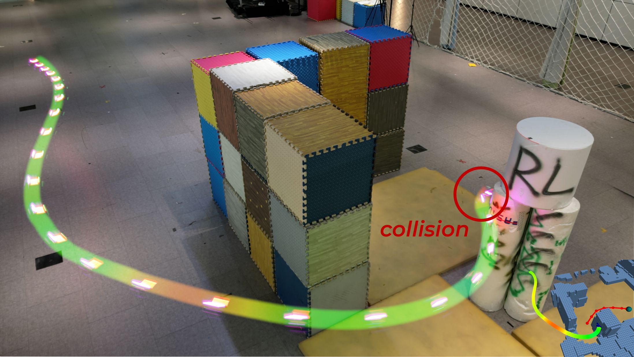
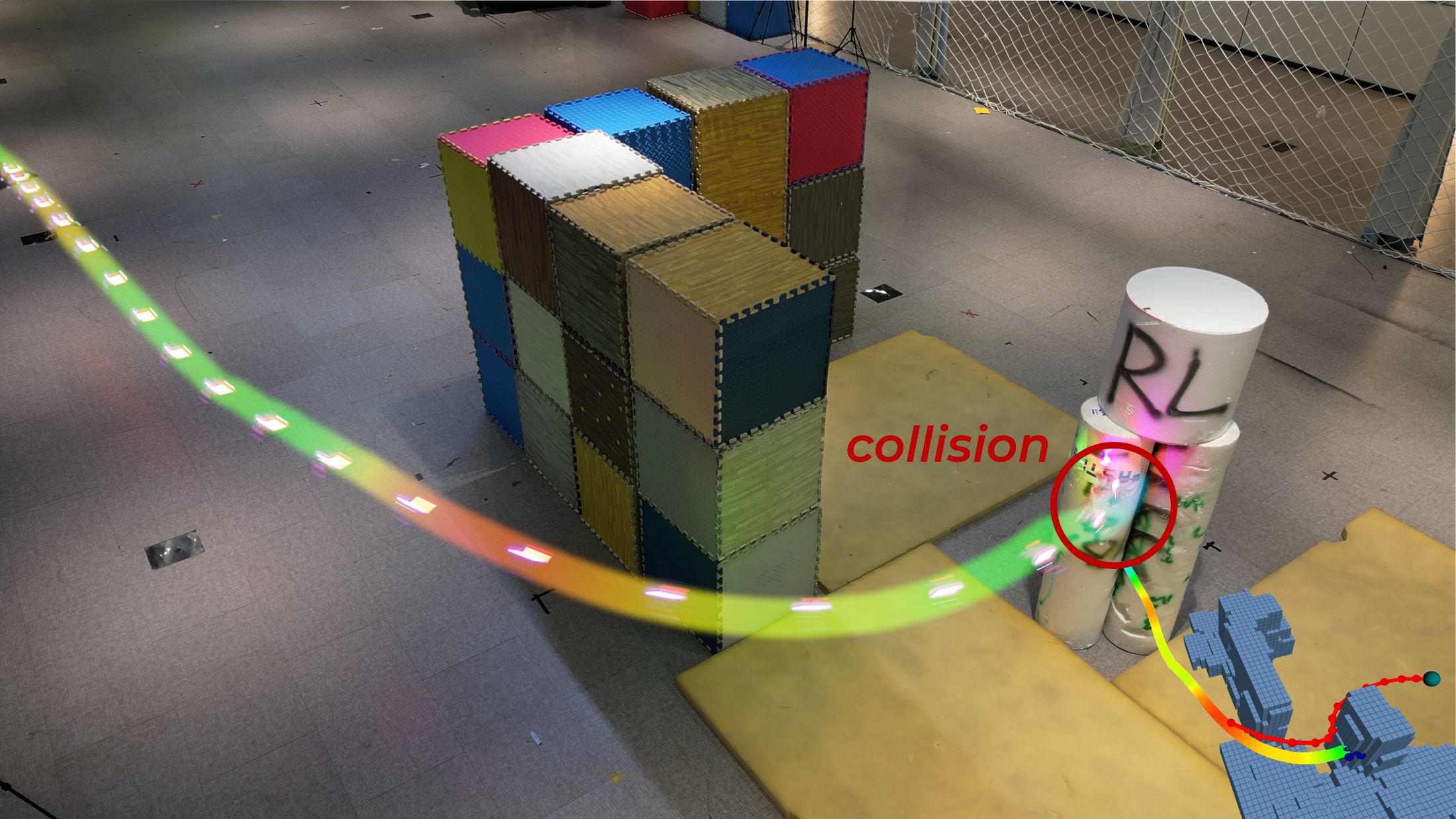
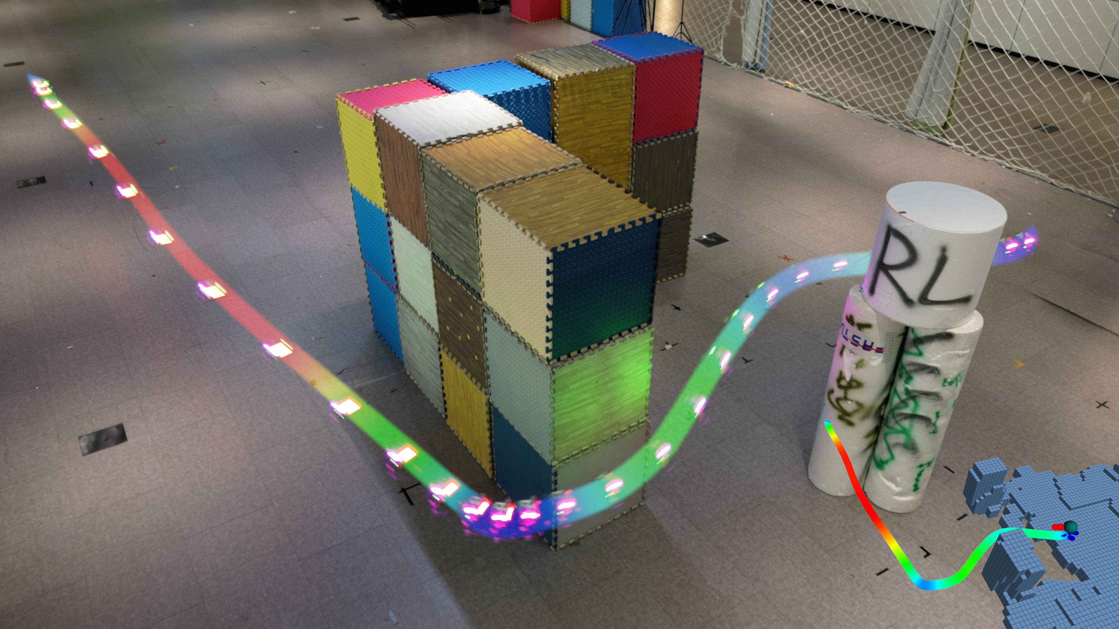
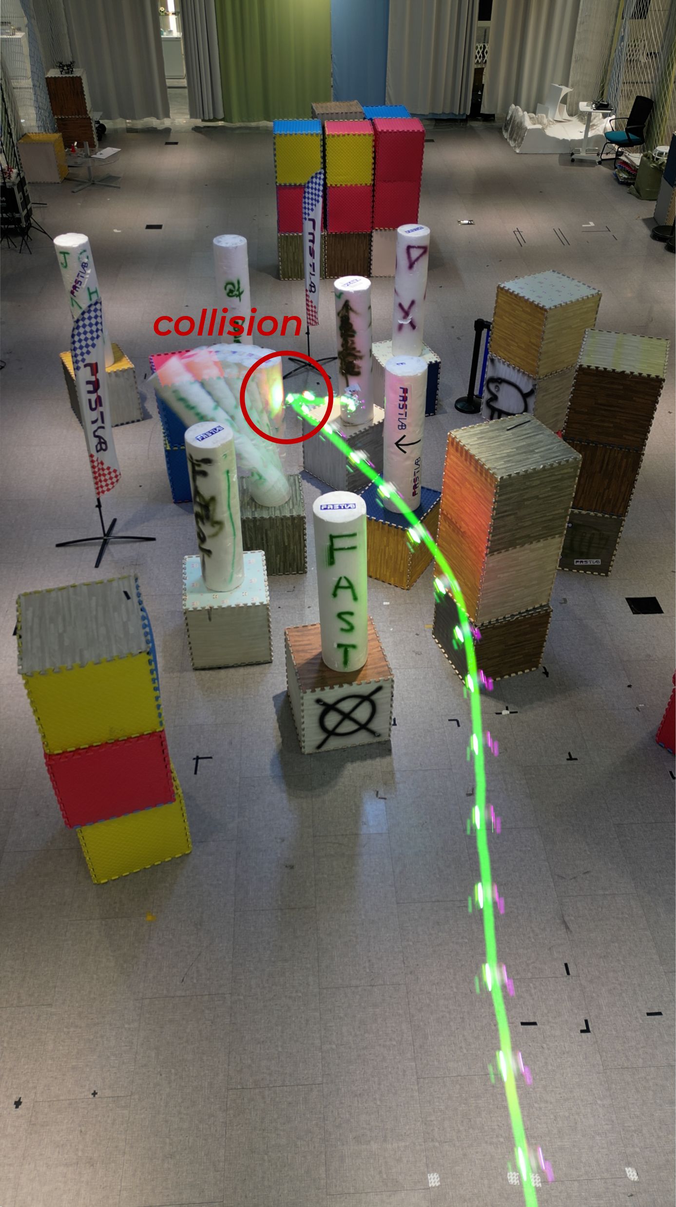
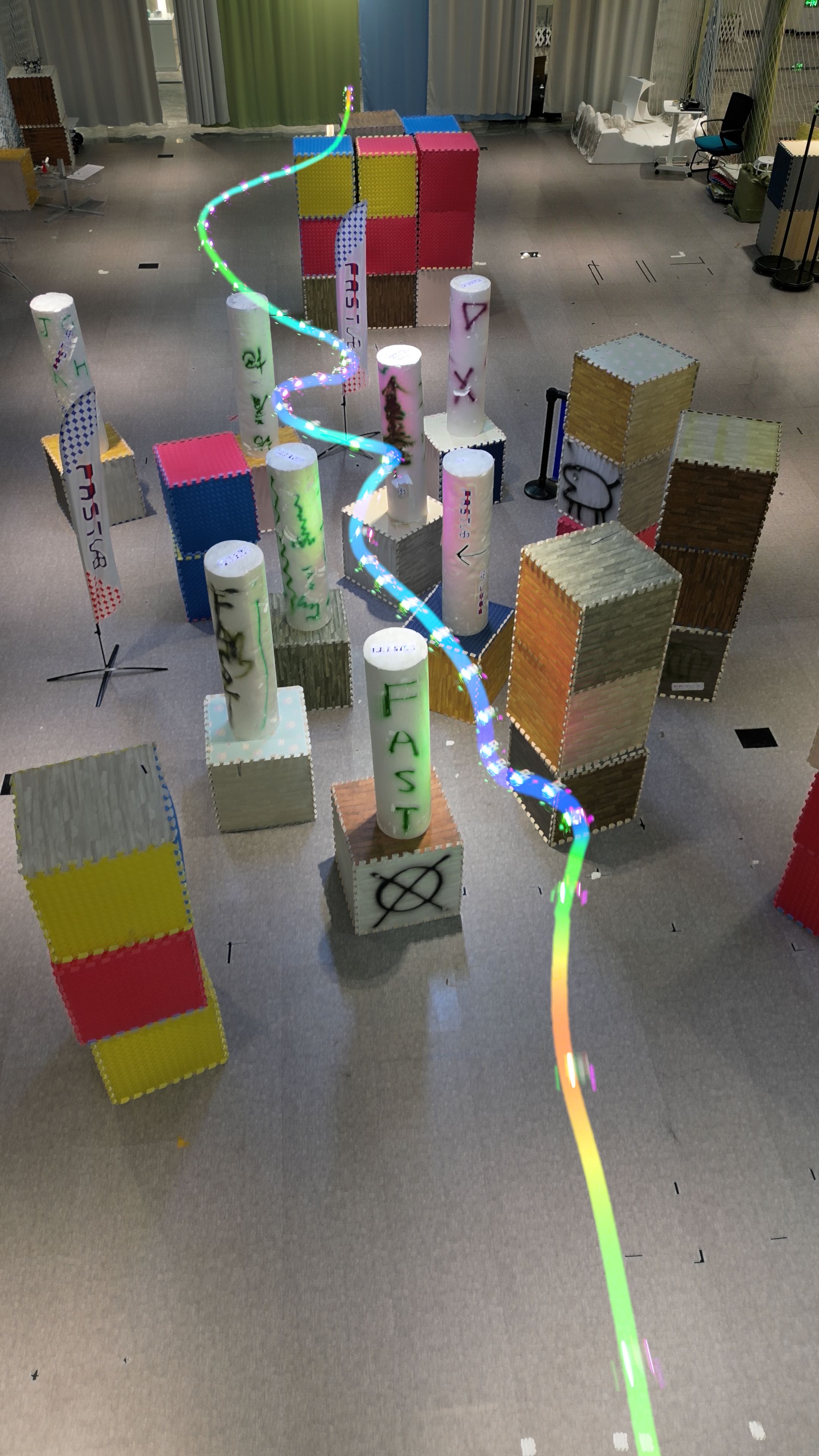
We validate the significance of agility adaptation in simulation, where the proposed approach outperforms both constant agility baselines and an alternative approach [23]. The policy can be directly deployed in the real world, leading to adaptive and safe flight in clutter, as shown in Fig. LABEL:fig:head.

II Related Work

II-A Adaptive Motion Planning

The works that have the most similar motivation to us are [23, 24, 25], which endeavor to alter agility for flight with model-based motion planners. In [23, 25], the authors impose the desired adaptive behavior by incorporating the velocity into trajectory planning via handcrafted cost functions. However, these cost functions are not expressive enough to comprehensively address the problem and inevitably lead to inflexible behavior. Methodologically, while we believe that powerful modeling-based approaches can be raised through more generalized and accurate formulations [26] and specialized computational techniques, learning-based approaches, if feasible, can serve as a simpler alternative. Zhou et al. [24] employ an online learning method based on Beyasian optimization to decide hyperparameter for trajectory planners. However, the painful convergence speed of Beyasian optimization makes their method incapable of adapting to a rapidly updating observation. We believe that an offline training mode, where the policy is determined before deployment, is more appropriate for the goal. Richter et al. [27, 28] formalize the problem of planning in an unknown environment and indicate the fundamental intractability in this formulation is on the belief that must capture the distribution of environments. Instead of directly operating on this distribution, the authors propose to learn a collision probability based on hand-coded features, while by striking out artificial features, our method is expected to achieve more flexible pattern recognition by jointly training perception and action modules.

As mentioned in section I, a work [16] released within weeks of our submission coincidentally studies agility-adaptive flight, but follows a different idea by training a policy directly outputting acceleration commands. In this approach, agility level is not explicitly incorporated into the action space. A specialized latent space used to maintain historical information is the key for the policy, which is achieved by a model-based mapping algorithm [29] in our framework. Our approach is tested in clutters (see Fig. LABEL:fig:head, Fig.5, and Fig. 10) that are much more complex compared to those in [16]. The unique success of our approach stems not only from the learned policy, but also the generalizability and safety of the model-based trajectory planner [17].

II-B Combining Learning and Model-based Planner for Navigation in Cluttered Environments

Recently, some works enhance traditional planning and control frameworks with learned policy to achieve more robust or efficient performance. Previous works [30, 15] employ imitation learning to direct predict local waypoints from visual input without geometric mapping for perceptive navigation. RL is also used to find an optimal policy [31] or a value estimator [32, 33] as additional modules for navigation without manual labeling. The most similar of these works to ours in terms of technical pipelines are [34, 35], which employ RL to regularize the parameters for a classical local planning algorithm, Dynamic Window Approach (DWA). However, our problem has distinct technical differences from these works. First, since we are concerned with combining agility and safety, we have to deal with sparse collision rewards. In many works, collision penalties can be densified by relaxing them as distance to the nearby obstacles. However, on the one hand, in this work, the spatial distribution of trajectories generated by the planner is almost independent of the output of RL policy, so penalizing distance-related metrics is not causally meaningful. On the other hand, especially in regions with densely distributed obstacles, penalizing distance is not a good reflection of our expectation on the behavior of vehicle and may introduce a short-sightedness. Second, the vehicle has to deal with limited field of view (FOV), rather than the near omnidirectional perception in [34, 35], which requires it to behave in a perception-aware manner. Moreover, while the above works are about ground robots navigating with low speed, our work contributes to agile flight systems, which requires the RL policy to cooperate with 3D perception and a much more complex modern planner backbone. Therefore, our work has a unique application contribution.

III Problem Formulation

We wish to control a flight vehicle through a prior unknown environment from one point to another with onboard perception. This problem can be formalized as a control problem in a partially observable Markov decision process (POMDP). We first overview the POMDP tuple $(S,A,T,R,\varOmega,O)$ and then formulate the problem.

• States $S$. The states space is divided into two parts, one is the controllable states $S^{c}$ which consists of the states of the vehicle such as $\boldsymbol{p}$ (position), $\boldsymbol{v}$ (velocity), $\boldsymbol{a}$ (acceleration), etc. The other part of $S$ is the environment $S^{e}$. In the context of our problem, $S^{e}$ can be described as the occupancy of the space, i.e., $s^{e}=\{0,1\}^{n}$.

• Actions $A$. Actions can be thought of control commands in a general sense such as the output of trajectory planning. For the class of flight vehicles considered in this paper, the specific form of the trajectory is reviewed in section IV-A.

• Conditional transition probabilities $T$. We assume that the dynamics of vehicle is known and deterministic, while the environment is static, i.e., $p\left(s^{e}|s^{e},a_{t}\right)=1$.

• The reward function $R$. As the topic of this paper suggests, our reward function is defined as maximizing agility and minimizing collision loss, where agility is defined as the velocity component of the trajectory

• Observations $\varOmega$. Observations include the state estimates of the vehicle, which is assumed to be perfect, and the partial observation of the environment $s^{e}$. The latter is limited by the FOV of the sensor (in this paper, the depth camera) and occlusion by obstacles.

• Conditional observation probabilities $O$. We preprocess the raw sensor input into a local occupancy map [29]. Thus, we are viewed as following the same assumptions about the conditional observation equations as [29].

The action at each moment is generated by a policy conditioned on the current observation and goal of navigation $g\in G$, i.e., $a_{t}\sim\pi\left(\cdot|o_{t},g\right)$. Our goal is to find the policy that maximize the expected cumulative return over time, i.e.,

$$\max_{\pi}\mathbb{E}_{s_{t+1}\sim p\left(\cdot|s_{t},a_{t}\right),a_{t}\sim\pi\left(\cdot|o_{t},g\right),g\sim p_{g}}\left[\sum\nolimits_{t}{\gamma^{t}r\left(s_{t},a_{t},g\right)}\right],$$ (1)

where $p_{g}$ is the distribution of $g$, and $\gamma$ is the discount factor.

IV Framework

Our framework involves a learned policy, which is donated as the agility policy $\pi^{\dagger}$, a model-based trajectory planner, and the standard perception and low-level control ends. The agility policy and model-based trajectory planner form a hierarchical policy to optimize (1).

IV-A Model-based Trajectory Planner

The trajectory planner receives the local geometric map and the states of the vehicle as inputs and generate a collision-free trajectory. The planner generates the trajectory by solving a constrained optimization in the form of

$$\min_{u\left(t\right)}\int_{0}^{T}{J\left(u\left(t\right)\right)+\rho\left(T\right)},\vspace{-0.1cm}$$ (2a)

s.t.

$$u\left(t\right)\in\mathcal{F},\ \ \forall t\in\left[0,T\right],$$ (2b)

$$\mathcal{G}\left(u\left(t\right)\right)\preceq\boldsymbol{0},\ \ \forall t\in\left[0,T\right],$$ (2c)

$$\mathcal{H}\left(u\left(t\right)\right)=\boldsymbol{0},\ \ \forall t\in\left[0,T\right],$$ (2d)

where $u\left(t\right)$ is the (high-level) planning quantities, $\rho:\left[\left.0,\infty\right)\right.\mapsto\left[0,\infty\right]$ the time regularization term, $\mathcal{F}$ the collision free region, $\mathcal{G}\left(\cdot\right)$ the dynamic constraints imposed by the physical limitation of the vehicle or users, and $\mathcal{H}\left(\cdot\right)$ summarizes the equality relations between the planning quantities and the states or control commands [36]. A widely used $u$ for underactuated multicopters consists of the flat-output space $z=\left(p_{x},p_{y},p_{z},\psi\right)^{\textnormal{T}}$ and the finite derivatives of it [11], where $(p_{x},p_{y},p_{z})^{\textnormal{T}}$ is the translation of the center of gravity and $\psi$ the yaw angle of the vehicle.

In the problem of navigation in cluttered environments, an inequality in (2c) represents the level of agility, such as $\left\|\boldsymbol{v}\right\|\leq\bar{v}$ or $\boldsymbol{v}\preceq\bar{\boldsymbol{v}}$, where $\bar{v}$ and $\bar{\boldsymbol{v}}$ are the imposed restriction on agility [7, 17]. For the generality of our description, we write such constraints uniformly as

$$h\left(\boldsymbol{v}\right)\preceq v^{\dagger}\vspace{-0.1cm}$$ (3)

without assigning them specific forms, where $v^{\dagger}$ is pre-determined as the planner solving for a trajectory.

Figure 1: Overview of the system with the hierarchical policy.

IV-B Hierarchical Policy Optimization

Traditionally, $v^{\dagger}$ is conservatively determined in advance based on the user’s observations of the environment to ensure safety. However, such an approach does not reasonably take advantage of the perception capabilities of the sensors, the performance of the algorithmic system, and the maneuverability of the vehicle. Instead, jointly optimizing the agility and trajectory to optimize (1) can further unlock the potential of the system.

We define a decomposition of the policy augmented with an auxiliary action $v^{\dagger}$

$$\pi^{\prime}(a^{\prime}|o,g)\coloneqq\pi^{\prime}(a,v^{\dagger}|o,g)=\pi^{\prime\prime}(a|v^{\dagger},o,g)\cdot\pi^{\dagger}(v^{\dagger}|o,g),$$ (4)

where the policy $\pi^{\prime}$ is decomposed as two hierarchical policies $\pi^{\prime\prime}$ and $\pi^{\dagger}$, the former of which is conditioned on the auxiliary action while the latter decides it. The action space of the original POMDP is augmented as a result of the introduction of an auxiliary action, i.e., $A^{\prime}=A\times V^{\dagger}$. However, no other part of the POMDP is changed, so we can define a hierarchical policy optimization problem

$$\begin{split}\max_{\pi^{\prime\prime},\pi^{\dagger}}\mathbb{E}_{a_{t}\sim\pi^{\prime\prime}(\cdot|v^{\dagger}_{t},o_{t},g),v^{\dagger}_{t}\sim\pi^{\dagger}\left(\cdot|o_{t},g\right)}\left[\sum\nolimits_{t}{\gamma^{t}r\left(s_{t},a_{t},g\right)}\right]=\\ \max_{\pi^{\dagger}}\max_{\pi^{\prime\prime}}\mathbb{E}_{a_{t}\sim\pi^{\prime\prime}(\cdot|v^{\dagger}_{t},o_{t},g),v^{\dagger}_{t}\sim\pi^{\dagger}(\cdot|o_{t},g)}\left[\sum\nolimits_{t}{\gamma^{t}r(s_{t},a_{t},g)}\right],\end{split}$$ (5)

where, for more concise writing, we omit the state and goal distributions in (1). This problem is equivalent to (1) in the sense that if $\pi$ and $\pi^{\prime}$ impose the same distribution on $a$ when conditioned on any $o\in O$ and $g\in G$, the objective function values of (1) and (5) are consistent.

Model-based trajectory planners [15, 12, 7, 17], after decades of development, can be regarded as a good approximation of the optimal $\pi^{\prime\prime}$ conditioned on a given $v^{\dagger}$. Therefore, only the outer-loop policy $\pi^{\dagger}$ needs to be learned. We use online model-free RL to learn this policy, which is detailed in the next section.

IV-C System Overview

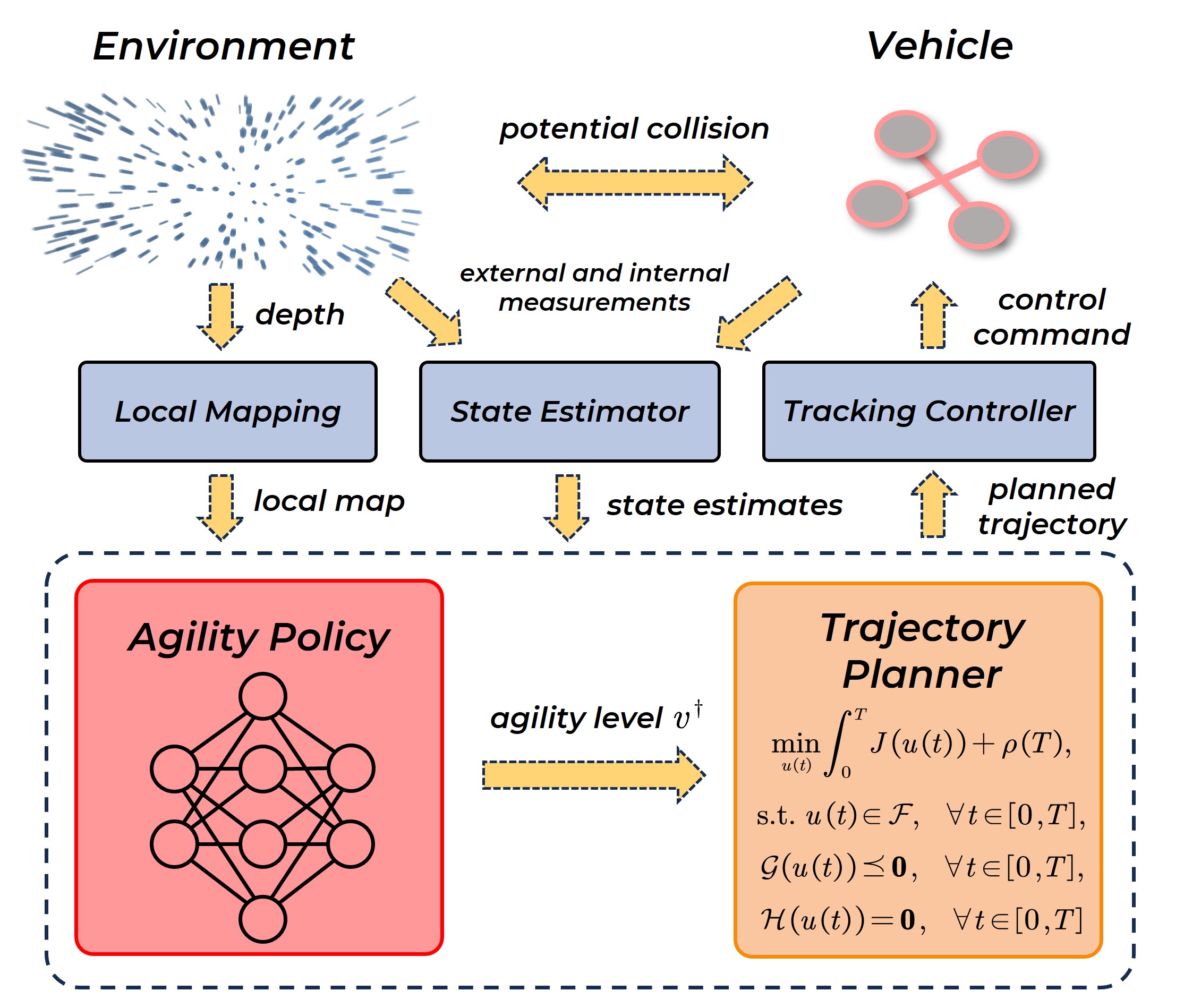
We conclude this section with an overview of the whole system, as illustrated in Fig. 1.

At the uppermost end of the system, the vehicle obtains partial observations of the environment via external sensors, which are used to provide state feedback (e.g., via the visual-inertial odometry (VIO)) and to construct local occupancy maps (e.g., from the depth camera). The local map and state estimates are fed to the RL policy and trajectory planner. We choose to use the occupancy map as the input of the RL policy instead of the raw sensory data because the training is performed in simulation, and such an approach deals with sensor noise through a model-based approach, i.e., the employed mapping algorithm, thus bridging the gap between simulation and reality in RL training.

At each time step $t$, the agility policy outputs a high-level planning instruction $v^{\dagger}_{t}$. The trajectory planner generates a trajectory $u$ in a horizon $[t,t+T]$ conditioned on $v^{\dagger}_{t}$. The discretization of the trajectory is treated as the action $a_{t}$ of the POMDP. The trajectory is tracked by a low-level controller and executed by the vehicle’s inner-loop controller. In our definition, the unknown environment as well as low-level controllers are treated as dynamics of the POMDP.

Figure 2: Illustration of the policy architecture and observation implementation. The figure shows the network architecture of policy, where actor and critic share the CNN encoder and fusion layer. We also highlight the 3D occupancy map where each cell is assigned a state, and its x-y profiles are sampled as the input of the network.

V Reinforcement Learning for Agility Policy

In this section, we detail how to efficiently and effectively learn the agility policy. Eq. (5) implies an approach to learn the agility policy, which treats the trajectory planner as part of the environment dynamics. An auxiliary POMDP is considered to learn $\pi^{\dagger}$, in which the action space is $V^{\dagger}$. In the following subsections, we present the implementation of each part of RL, where a couple of pre-training-fine-tuning reward functions are the keys to a successful training.

V-A Policy Representation

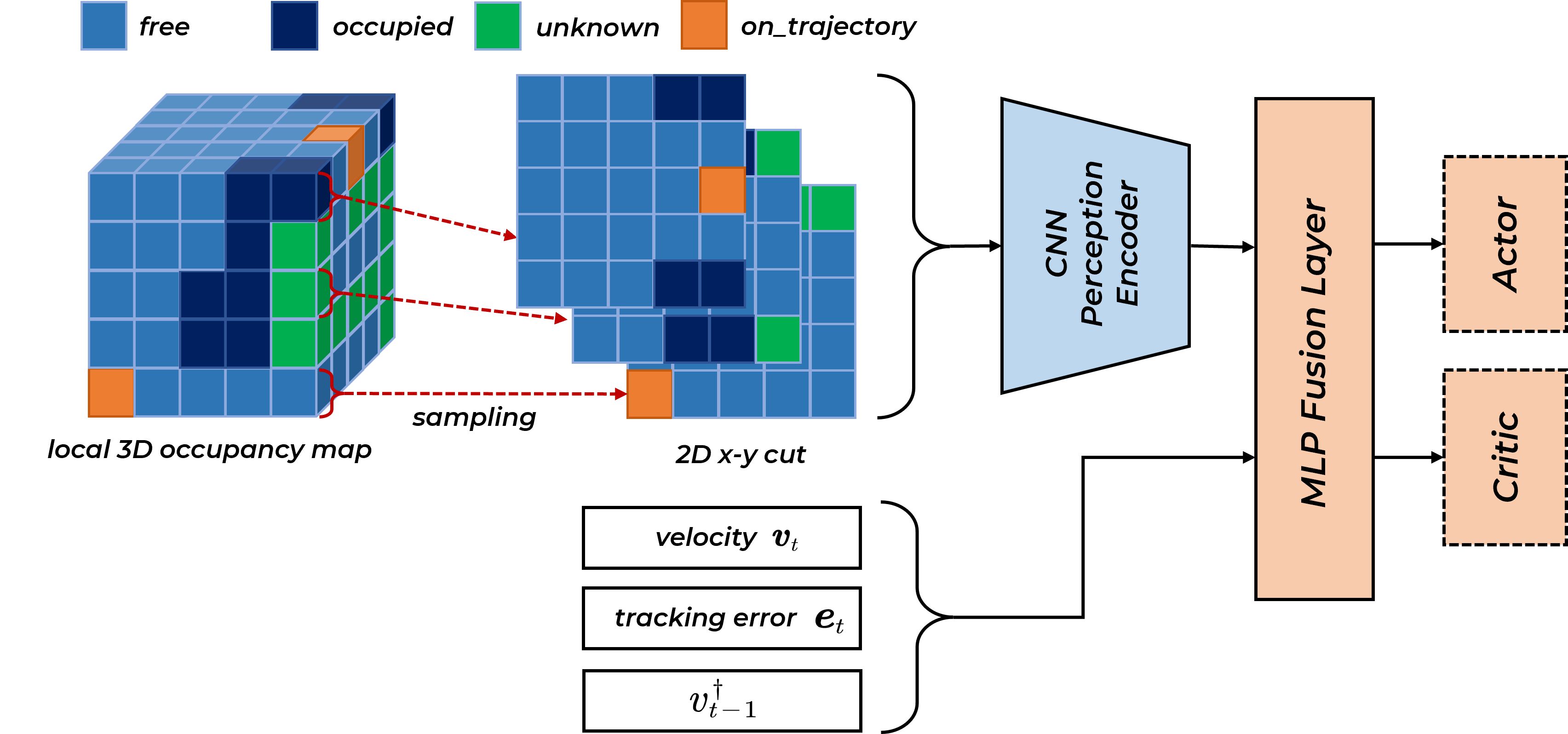
We represent policy and value functions using a branch of partially shared neural networks, as illustrated in Fig. 2. The networks share a perception encoder consists of convolution neural networks (CNNs) and a fusion layer implemented with multilayer perceptron (MLP). We implement the CNN encoder with 4 layers whose [channel number, kernel size, stride, padding] are [5,5,3,2], [32,3,2,1], [48,3,2,1], and [64,3,1,0]. The result of the CNN encoder is flattened and concatenated into the inputs of the MLP fusion layer. The output dimension of the MLP layer is 64. The actor and critic networks are both implemented as MLPs with 2 hidden layers having 64 and 32 units, respectively.

V-B Observation Space

As shown by (5), in principle, $\pi^{\dagger}$ should be conditioned on the observations and the goal of navigation. However, as illustrated in Fig. 2, we employ a more practical input which consists of the local 3D occupancy map $\boldsymbol{m}_{t}$, the current velocity $\boldsymbol{v}_{t}$, the current tracking error $\boldsymbol{e}_{t}\coloneqq\boldsymbol{p}_{t}-\hat{\boldsymbol{p}}_{t}$, where $\boldsymbol{p}_{t}$ and $\hat{\boldsymbol{p}}_{t}$ are the true and desired position of the vehicle, respectively, the agility decision at the last time step ${v}^{\dagger}_{t-1}$, and a pre-planned trajectory at the current time step generated according to ${v}^{\dagger}_{t-1}$ and $o_{t}$, which will not be executed by the controller.

The pre-planned trajectory serves two purposes. First, it expresses the current position of the vehicle in the local map as well as the local target chosen by the trajectory planner according to the global goal $g$. Second, since agility has little effect on the spatial distribution of the trajectory, we can use this pre-planned trajectory as a spatial approximation of the trajectory to be planned, and therefore alert the perceptual part of the policy as to which regions in the local map are important.

We correlate the trajectory and the 3D local map by ’drawing’ the former on the latter, as illustrated by Fig. 2. Specifically, each cell in the occupancy map is assigned one of four states: free, occupied, unknown, and on_trajectory. The state unknown is set to trigger perception-aware behaviors. For more efficient and easier learning, we sample the trajectory with time interval $\delta t$, keeping only the x-y 2D cut of the 3D map corresponding to the sampled point on the trajectory as input to the network, which is illustrated in Fig. 2.

V-C Termination

We define two cases of termination. One is when the vehicle is in an unsafe state, i.e., the vehicle is judged in the emergency_stop or collided state, which is determined by the state machine in a modern motion planning system [7, 17]. The other occurs when the planning solution procedure does not finish in a valid time, which is often due to too high level of agility allowed in the previous time steps, so that the vehicle is too close to a suddenly appearing obstacle under the perception latency and thus the planner fails to plan a feasible trajectory.

Figure 3: Example illustration of the naive estimate of the danger level. The blue blocks are the perceived local occupancy map. (a) A safe case where small number of obstacles are far from the vehicle. (b) A mild case. (c) A dangerous case where an obstacle is close to the vehicle.

V-D Reward Function

As described in section III, we design the reward function to maximize agility and minimize collision loss. For practical considerations, we further divide the reward function into four parts: the agility term, the smoothing term, the tracking error term, and the (sparse) collision term:

$$r=r_{\textnormal{agility}}+r_{\textnormal{smoothing}}+r_{\textnormal{error}}+r_{\textnormal{danger}},\vspace{-0.1cm}$$ (6)

where the specific forms of the smoothing, tracking error and collision terms are

$$r_{\textnormal{smoothing}}=-\lambda_{\textnormal{smoothing}}\|v_{t}^{\dagger}-v_{t-1}^{\dagger}\|^{2},\vspace{-0.2cm}$$ (7)

$$r_{\textnormal{error}}=-\lambda_{\textnormal{error}}\min\left\{\|\boldsymbol{e}_{t}\|,e_{\max}\right\}^{2},\vspace{-0.1cm}$$ (8)

$$r_{\textnormal{danger}}=\begin{cases}-\lambda_{\textnormal{danger}}\|\boldsymbol{v}_{t}\|^{2}&\textnormal{(when the episode is terminal)}\\ 0&\textnormal{(otherwise)}\\ \end{cases},\vspace{-0.1cm}$$ (9)

for some $\lambda_{\textnormal{smoothing}}>0$, $\lambda_{\textnormal{error}}>0$, and $\lambda_{\textnormal{danger}}>0$.

However, since $r_{\textnormal{danger}}$ is highly sparse and stochastic, this form of reward is difficult to learn with for general RL algorithms, especially when embedded in a complex modern trajectory planner. Our key finding here is that with a two-stage reward design in a pre-training-fine-tuning training pipeline, learning can take place efficiently and effectively. The only term that differs between the first and second stages is $r_{\textnormal{agility}}$, which is detailed in the following.

V-D1 A human knowledge-based, dense reward function for pre-training

The agility reward in the first stage is defined as follows:

$$r_{\textnormal{agility}}=\begin{cases}\lambda_{\textnormal{agility}}^{1}(\phi_{t}^{1}-\|\boldsymbol{v}_{t}\|)&\left(\phi_{t}^{2}>2\right)\\ \lambda_{\textnormal{agility}}^{2}(\|\boldsymbol{v}_{t}\|-\phi_{t}^{1})&\left(\phi_{t}^{2}<1\right)\\ \lambda_{\textnormal{agility}}^{3}\|\boldsymbol{v}_{t}\|&\textnormal{(otherwise)}\\ \end{cases},\vspace{-0.1cm}$$ (10)

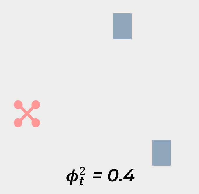
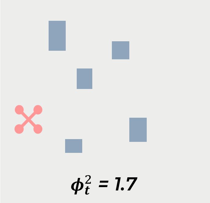
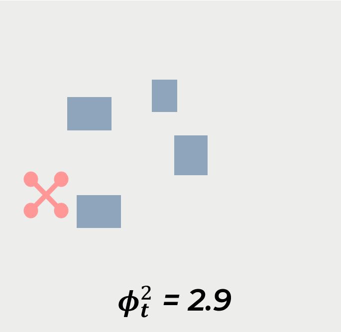
where $\lambda_{\textnormal{agility}}^{i}>0$ for $i\in\left\{1,2,3\right\}$, $\lambda_{\textnormal{agility}}^{2}>\lambda_{\textnormal{agility}}^{3}$, and $\phi_{t}^{i}$s, for $i\in\left\{1,2\right\}$, are handcrafted feature values encoding the obstacle distribution. Specially, $\phi_{t}^{i}$s are normalized linear combinations of the distance to the nearest obstacle, volume of the obstacle, and number of obstacles at current time, some example of which are illustrated in Fig. 3.

In (10), $\phi_{t}^{1}$ is designed to shape the reward function smoother with a zero mean, while $\phi_{t}^{2}$ is a naive estimate of the level of danger by human knowledge. The first case in (10) serves as a dense smoothing of the collision penalty.

V-D2 An objective reward for fine-tuning

In the second stage, we restore the intent of the agility reward, which is to encourage greater agility, as follows:

$$r_{\textnormal{agility}}=\lambda_{\textnormal{agility}}^{3}\|\boldsymbol{v}_{t}\|.\vspace{-0.1cm}$$ (11)

VI Training Setup and Implementation

VI-A System Setup

We choose a state-of-the-art model-based trajectory planner, EGO-planner [17], as the backbone. The agility constraint is imposed in the form of $\left\|\boldsymbol{v}\right\|\leq\bar{v}$. The local mapping algorithm is implemented based on [29]. The vehicle is equipped with a forward-facing camera that can measure depth with a FOV of 87^∘ (horizontal) $\times$ 58^∘ (vertical) and a valid/trusted depth range from $0.28$m to $5$m. The refreshing frequency of the depth data is 15 Hz. A PID controller running at 50 Hz is used for position tracking.

The agility policy runs at 10 Hz. Conceptually, trajectory planning is required after each agility policy output, but too frequent replanning increases the situations of triggering the emergency_stop state in practice, as well as increasing the computational overhead. Therefore, we design a criterion to determine whether replanning is imposed by the agility policy output, and if this criterion is not met, the planner follows its original implementation of replanning rules. In particular, if $v_{t}^{\dagger}-v_{t-1}^{\dagger}\in\left[-0.3,0.5\right]$m/s, we do not impose a replanning of the trajectory planner.

VI-B Training Environment

We train the policy in a customized simulator. Unlike general simulation environments, the simulator does not stop the clock while solving for the action (i.e., trajectory planning) in our simulation environment. Meanwhile, the sensory data is updated asynchronously with the action. This is to simulate one of the most important factors limiting agility, the perception latency, i.e., the time interval between perception and execution of an action. Another crucial factor that limits agility, the imperfect performance of trajectory tracking, is also embedded in the environment by setting up the actual PID tracking controller for the vehicle, as described earlier.

Figure 4: Example illustration of environments for training. Areas in blue represent the space filled with obstacles.

VI-C Training Implementation

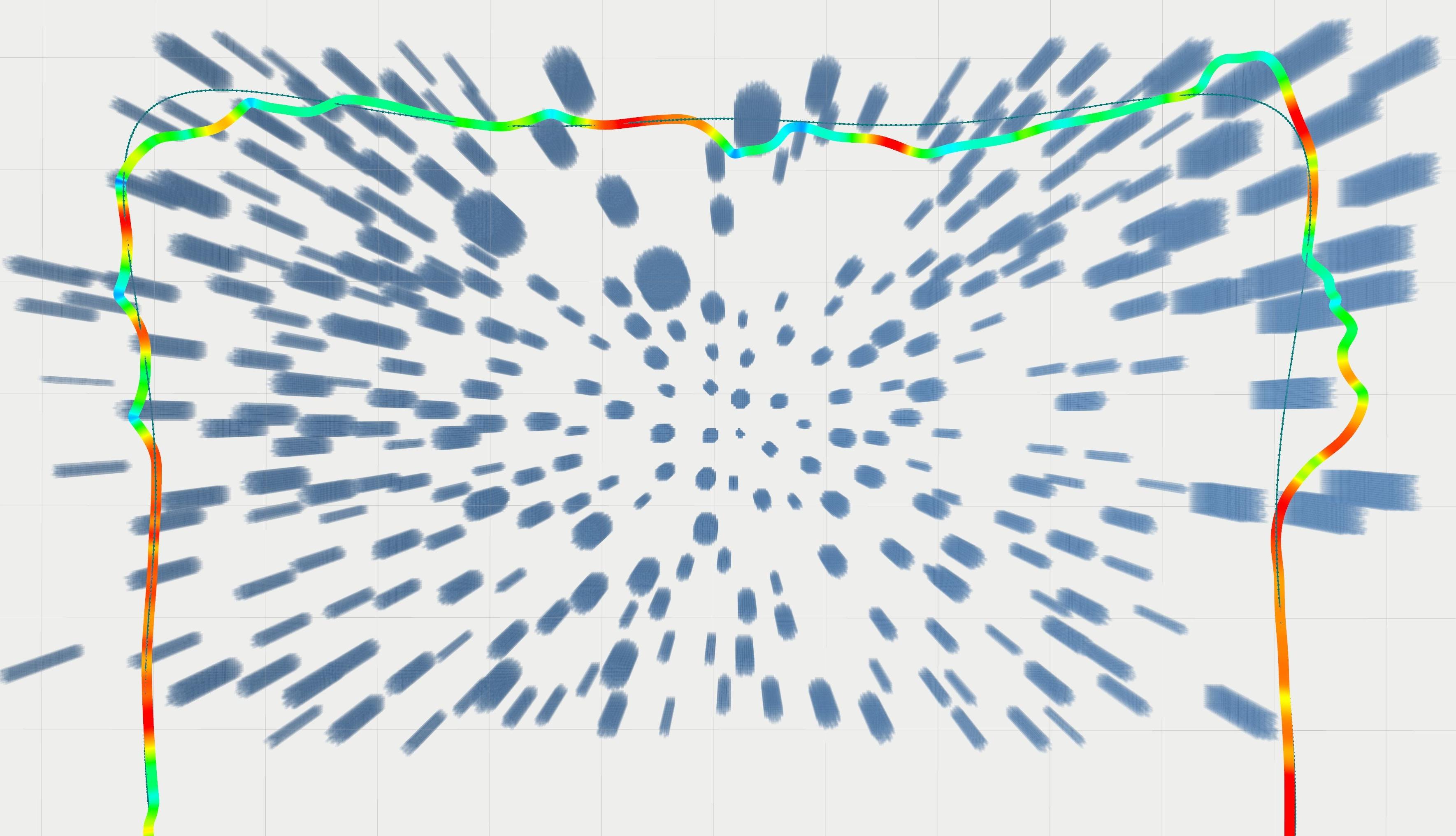
The policy is learned with the soft actor-critic (SAC) algorithm [37]. Prioritized experience replay (PER) [38] is also applied to mitigate the sparse failure mode problem in a general way. We train the policy in multiple scenarios with variable obstacle distributions, some of which are shown in Fig. 4. We freeze the CNN encoder in the second stage of training, considering that the first-stage reward design encourages the encoder to extract features that can flexibly respond to different patterns of the obstacle distribution.

Figure 5: Velocity distribution along the trajectory in different setups. The dark green curves are the reference trajectory. The colorful curves are the trajectory that the vehicle passes over, where the color represents the velocity. (a) An example result of the proposed approach. (b) An example result of the constant agility ${v}^{\dagger}=2$m/s. (c) An example result of the intermediate model before fine-tuning.

Figure 6: Statistical results of different setups. Success rates are computed on 50 trials for each setup. The light blue dashed lines connect the statistics at different levels of constant agility, indicating the inherent capability of the system. Average velocities are computed as the average of success trials in the 50 trials.

VII Experiments

VII-A Simulation Experiments

We benchmark three approaches in the simulation experiments: (i) the proposed ’agility policy + model-based planner backbone’, (ii) the backbone planner EGO-planner with constant agility (i.e., constant ${v}^{\dagger}$), and (iii) the handcrafted cost function-based (non-learning) environmental adaptive planner EVA-planner [23], where the default parameters in the cost function are used, and all parameters that EGO-planner shares with it are set equal to those of EGO-planner.

Figure 7: Comparison of the proposed approach and EVA-planner. The colorful curves are the trajectory that the vehicle passes over, where the color represents the velocity. The marked average velocity is computed on 30 trials. (a) Illustration of the trajectory generated by the proposed approach. (b) Illustration of the trajectory generated by EVA-planner.

Figure 8: Illustration of perception-aware behaviors of the learned policy and comparison with EVA-planner. The colorful curves are the trajectory that the vehicle passes over, where the color represents the velocity. The dark gray grid is the built local map. (a) Illustration of the scenario, where the dark green line is the reference trajectory. (b) Behaviors of the proposed approach. (c) Behaviors of EVA-planner, where the yaw angles and FOV boundaries are shown to explain the failure.

VII-A1 Comparison of the proposed framework with constant agility baselines and ablation tests

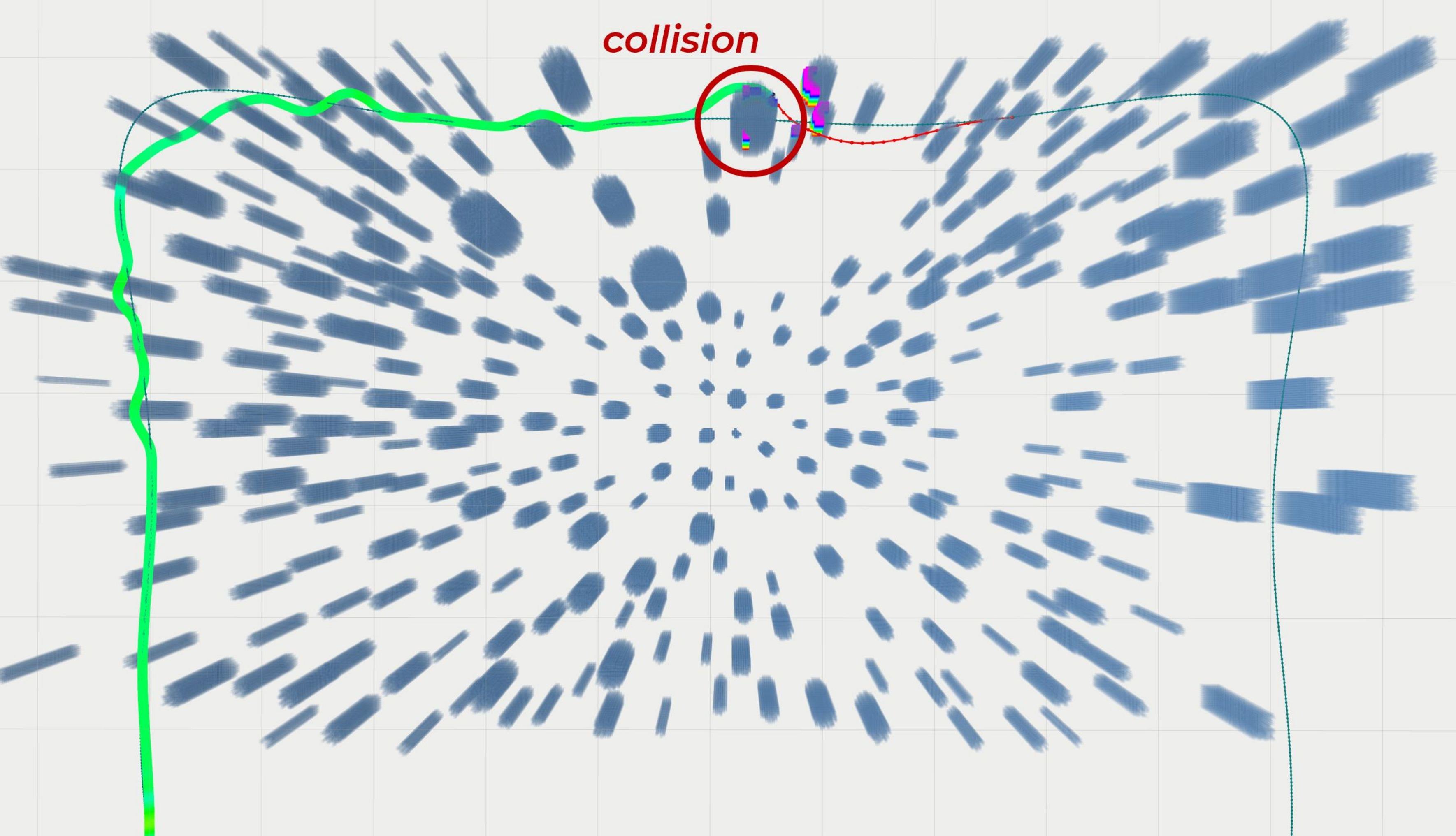
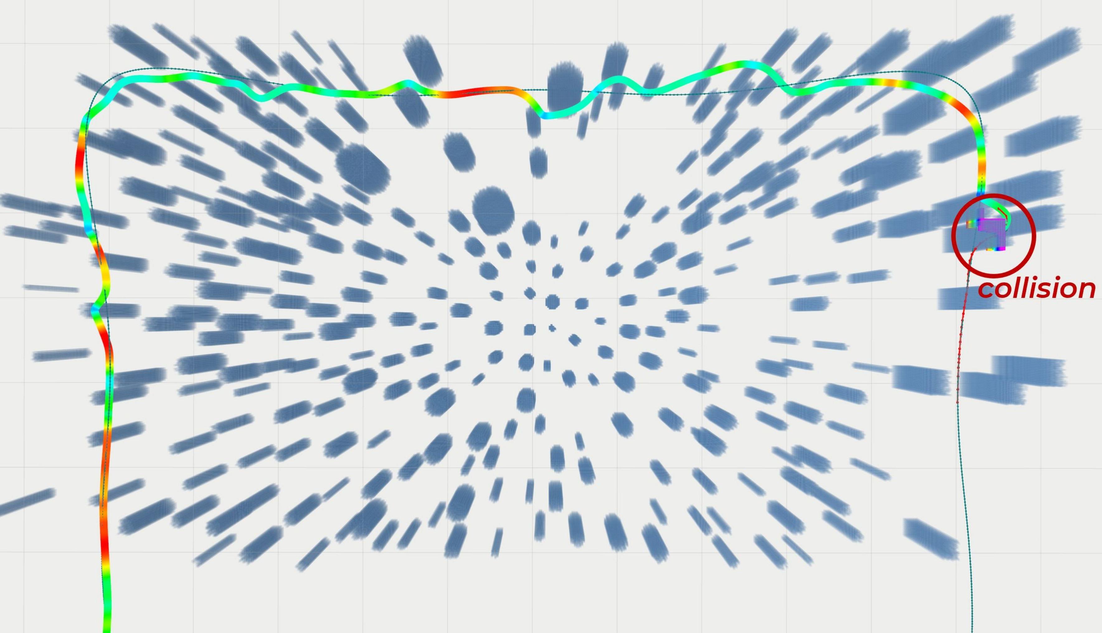
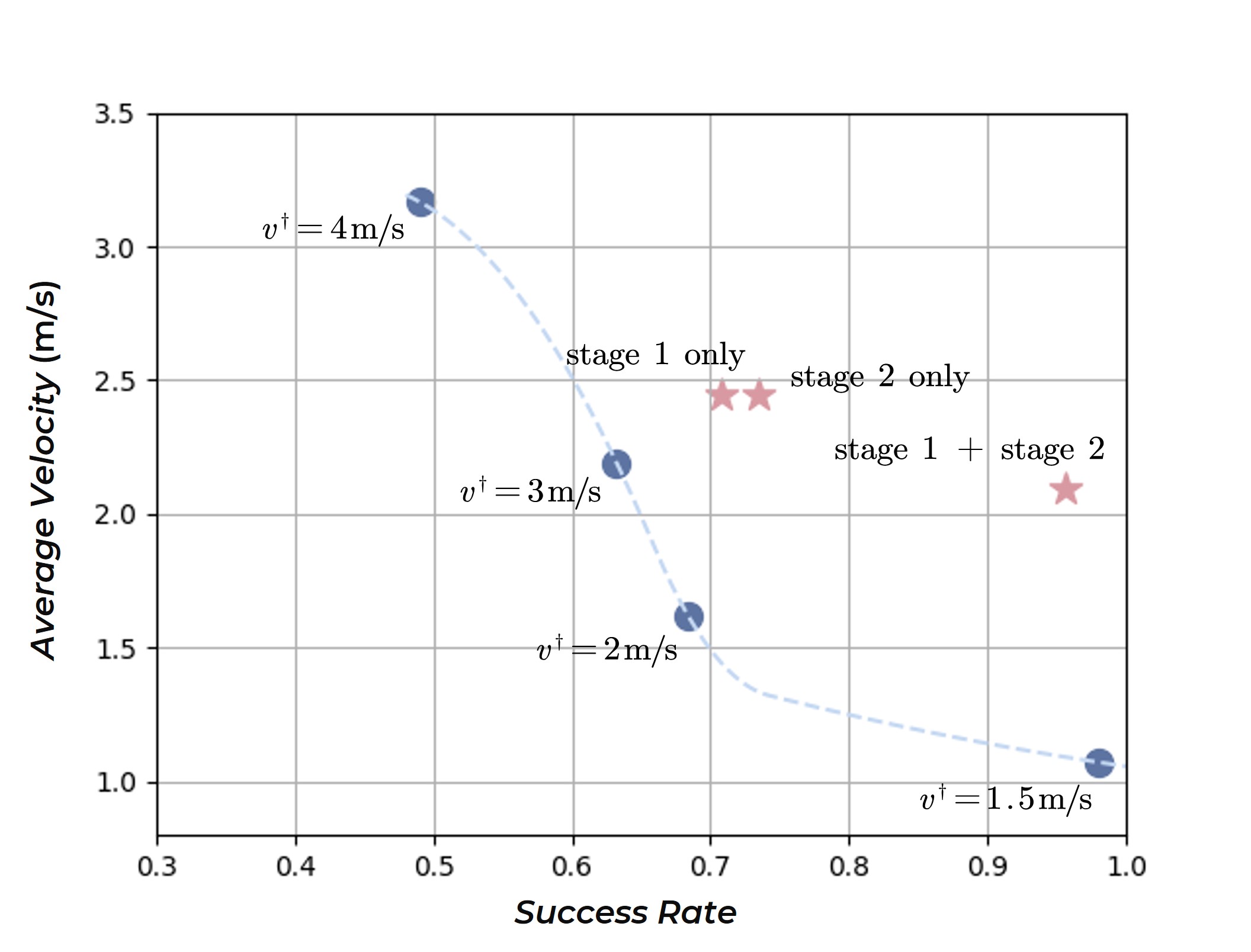
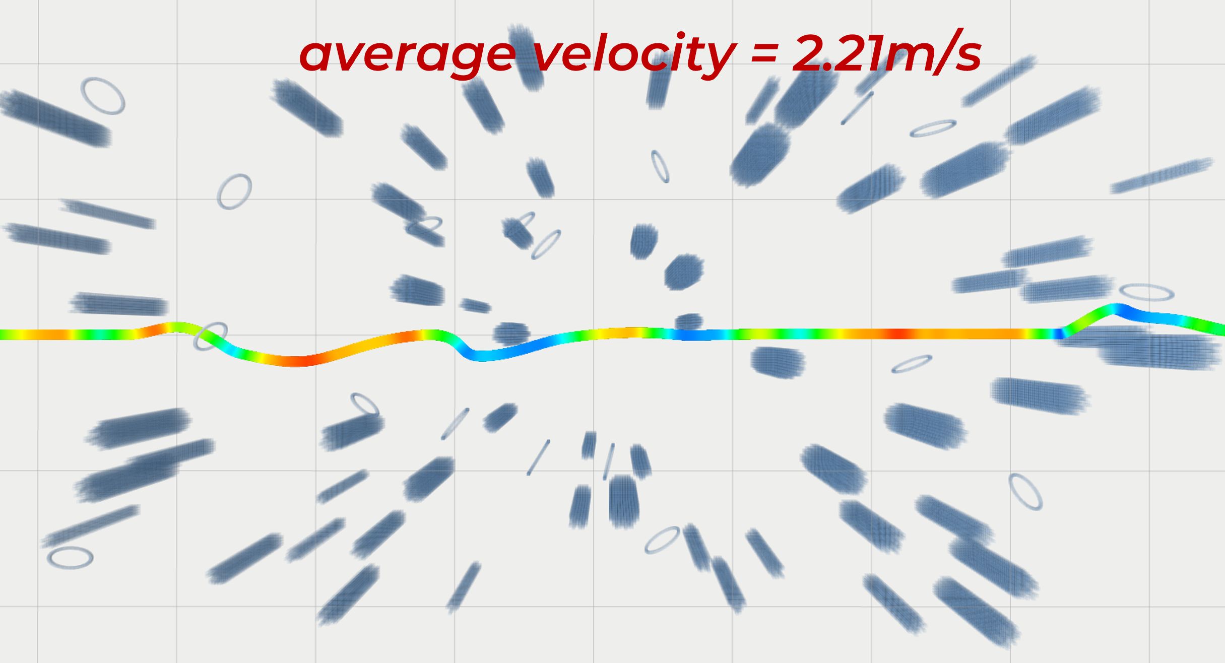
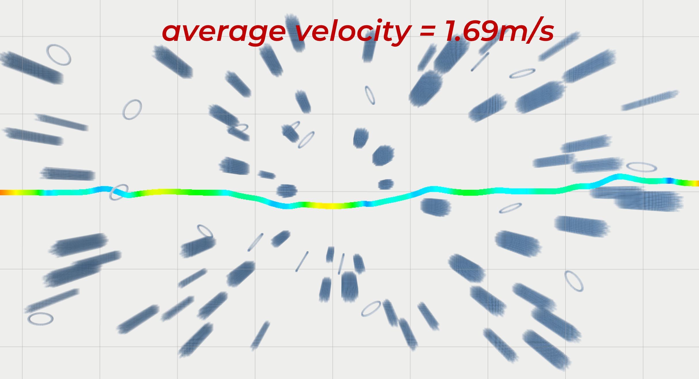
The first two setups are evaluated in a challenging environment as shown in Fig. 5, where obstacles of different densities, sizes, and appearances are unevenly distributed. The evaluation environment is never seen when training. In Fig. 6, we report the statistical results of traversal velocity in success cases and the success rate which is defined as the proportion of trials that complete the entire track. A trial is judged to be ’terminal’ with the same criteria as during training. In Fig. 5, we visualize the trajectories and velocities at every moment of the proposed approach and the baselines. Since the trajectory generation backbone of EVA-planner cannot always effectively generate feasible trajectory in such a complex environment, it is not fair to include it in this statistical result, so we ignore the results of EVA-planner in Fig. 6.

The statistics show that as ${v}^{\dagger}$ is set higher, the success rate decreases, creating a sloping downward performance curve in Fig. 6. Such performance curves capture the inherent performance of the integration of physical (e.g., sensors equipped) and algorithmic (e.g., the planning and control framework) systems. Although under the performance constraints of the system, by dynamically configuring the agility based on observations, the vehicle combines the exploitation of agility and safety guarantees. Specifically, it can be seen in Fig. 6 that the policy learned with both the reward stages achieves similar success rate as the lowest agility case where ${v}^{\dagger}=1.5$m/s, but also exhibits considerable traversal speeds to efficiently complete the track. In contrast, a relatively aggressive constant agility ${v}^{\dagger}=2$m/s can frequently lead to emergency stops or collisions in areas with dense obstacles or local occlusion, as shown in Fig. 5.

In Fig. 6, we also show the performance of the policies trained only with either the first stage (reward (10)) or the second stage (reward (11)). The results indicate that although the final policy can successfully improve the overall performance of the system, the policy trained with only the first stage does not exhibit substantial improvement. This result is not so surprising since the reward scheme of the first stage of training does not reflect the objective values and impose inaccurate human knowledge. On the other hand, the necessity of the first training stage is reflected by the inferiority of the performance rendered by the policy trained directly with sparse (but objective) rewards in Fig. 6.

VII-A2 Comparison of the proposed framework with EVA-planner and an example case of perception-aware behaviors

EVA-planner tends to plan (sometimes overly) conservative velocities, which can be seen in Fig. 7, while the proposed approach makes better use of the vehicle’s maneuverability, at the cost of large changes in velocity, as seen in Fig. 7.

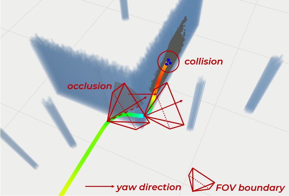
More importantly, since the hand-designed cost function of EVA-planner does not capture some aspects of the problem, such as the necessity of risk and perception awareness, an unsafe decision may be output by the planner. An example is illustrated in Fig. 8. In such a case, the agility policy learns to behave cautiously when the vehicle plans to turn its head into area out of its perception range, which is caused by occlusion of a corner and attitude angle changes. In contrast, EVA-planner plans an unsafe velocity due to its illusion that there are no obstacles nearby, which is caused by occlusion, yaw angle changes, and perception latency. However, such perception-aware behaviors does not always occur in the policy obtained using only the first stage of reward. An example is shown in Fig. 5, where acceleration at a corner causes the vehicle to collide.

Figure 9: Flight to avoid a wall-like obstacle with a hidden pillar. The planned trajectory (red curve), the executed trajectory (colored curve), and the local map (blue) are indicated in the bottom right corner of each figure. (a) Flight with constant agility ${v}^{\dagger}=2.5$m/s. (b) Flight with constant agility ${v}^{\dagger}=3.5$m/s (c) Flight with agility adaptation.

Figure 10: Flight through dense and large-sized obstacles. (a) Flight with constant agility ${v}^{\dagger}=2.5$m/s. (b) Flight with agility adaptation.

VII-B Real-World Experiments

We deploy the policy on a micro drone with a size of $17$cm$\times 17$cm$\times 10$cm. The drone is equipped with an onboard RealSense D430 depth camera. Computation/inference is performed on an onboard Jetson Orin NX module. We use the NOKOV motion capture system and a VIO to obtain the state estimates respectively in indoor and outdoor scenarios. The parameter setup is aligned with that in section VI-A.

VII-B1 Wall-like obstacles with an obstacle hidden behind

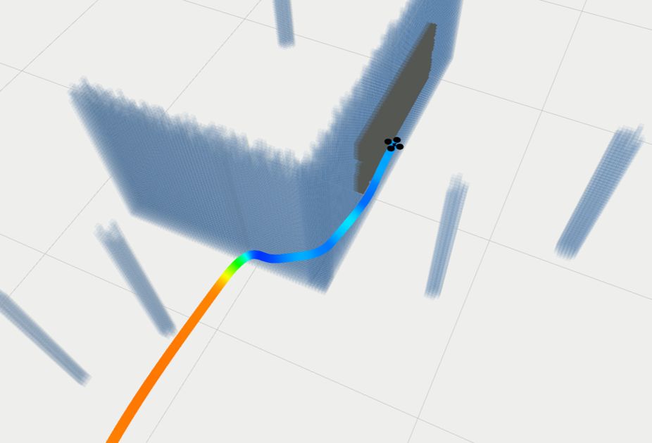
We first test the policy in a representative scenario where a wall-like obstacle blocked near half of the vehicle’s FOV, and only after the vehicle avoids the corner could it observe the obstacle immediately afterward.

In such a scenario, the policies set to constant agility levels, e.g., in Fig. 9, $v^{\dagger}=2.5$m/s and $v^{\dagger}_{t}=3.5$m/s, are able to plan a collision-free trajectory in most of the trials, which is due to the efficiency of the EGO-planner itself. However, the planned trajectory is far from being able to be perfectly tracked by the low-level controller since the trajectory requires sudden changes of motion, which leads to collisions. In this case, the trajectory optimization cost function of EGO-planner [17, Eq. (8)] (somehow) sacrifices dynamical feasibility to ensure a collision-free trajectory, but still fails to spare the vehicle.

In contrast, as shown in Fig. 9, after plugging the learned policy, the vehicle exhibits perception-aware behaviors, slowing down in the corner of the wall and recovering agility as more extents of the hidden obstacle is observed, until it eventually slows down to stop at the goal.

VII-B2 Artificial Clutters

We evaluate the policy in an artificial scenario shown in Fig. 10. In this scenario, a dense clutter and a large-sized obstacle exist in the first and second half of the scene, respectively. The constant agility policies, as shown in the Fig. 10, fails in half of the trials due to planning time overruns, the occurrence of emergence stops (as explained in section V-C), and also collisions caused by the same reason as that described in the previous subsection. With the learned module, the policy reasonably exploits agility in open areas, and also behaviors cautiously among dense obstacles, as shown in Fig. 10, thus ensuring success in almost all trials.

VII-B3 Natural Clutters

We also evaluate the policy in natural clutters as shown in Fig. LABEL:fig:head, where the highly uneven environment triggers rich patterns of vehicle’s behavior. Despite the particularly complex environment, our policy exhibits aggressive behavior in open areas (Fig. LABEL:fig:head, top left and bottom right), but stays cautious to ensure safety when crossing narrow gap (Fig. LABEL:fig:head, top right) or among obstacles (Fig. LABEL:fig:head, bottom left).

VIII Conclusion

We proposed a hierarchical learning and planning framework for agility adaptive flight in cluttered environments. On the one hand, the hierarchical framework allows the system to obtain a strong overall performance thanks to the existing powerful model-based trajectory planner. On the other hand, by doing so, we complement the ’missing jigsaw puzzle’ in traditional trajectory planners, thus unlocking the potential of the algorithmic system while freeing humans from hand-tuning labor. We see this as a necessary step towards a self-closing loop for autonomous flight vehicles.

References

- [1] T. Yoon, R. B. Geary, A. A. Ahmed, and R. Shadmehr, “Control of movement vigor and decision making during foraging,” Proceedings of the National Academy of Sciences, vol. 115, no. 44, pp. E10 476–E10 485, 2018.
- [2] A. M. Wilson, J. Lowe, K. Roskilly, P. E. Hudson, K. Golabek, and J. McNutt, “Locomotion dynamics of hunting in wild cheetahs,” Nature, vol. 498, no. 7453, pp. 185–189, 2013.
- [3] P. A. Bednekoff and S. L. Lima, “Randomness, chaos and confusion in the study of antipredator vigilance,” Trends in Ecology & Evolution, vol. 13, no. 7, pp. 284–287, 1998.
- [4] R. Wheatley, M. J. Angilletta Jr, A. C. Niehaus, and R. S. Wilson, “How fast should an animal run when escaping? an optimality model based on the trade-off between speed and accuracy,” Integrative and comparative biology, vol. 55, no. 6, pp. 1166–1175, 2015.
- [5] P. Henningsson, “Flying through gaps: how does a bird deal with the problem and what costs are there?” Royal Society Open Science, vol. 8, no. 8, p. 211072, 2021.
- [6] J. D. Smith, W. E. Shields, and D. A. Washburn, “The comparative psychology of uncertainty monitoring and metacognition,” Behavioral and brain sciences, vol. 26, no. 3, pp. 317–339, 2003.
- [7] B. Zhou, F. Gao, L. Wang, C. Liu, and S. Shen, “Robust and efficient quadrotor trajectory generation for fast autonomous flight,” IEEE Robotics and Automation Letters, vol. 4, no. 4, pp. 3529–3536, 2019.
- [8] M. O’Connell, G. Shi, X. Shi, K. Azizzadenesheli, A. Anandkumar, Y. Yue, and S.-J. Chung, “Neural-fly enables rapid learning for agile flight in strong winds,” Science Robotics, vol. 7, no. 66, p. eabm6597, 2022.
- [9] Y. Song, A. Romero, M. Müller, V. Koltun, and D. Scaramuzza, “Reaching the limit in autonomous racing: Optimal control versus reinforcement learning,” Science Robotics, vol. 8, no. 82, p. eadg1462, 2023.
- [10] E. Kaufmann, L. Bauersfeld, A. Loquercio, M. Müller, V. Koltun, and D. Scaramuzza, “Champion-level drone racing using deep reinforcement learning,” Nature, vol. 620, no. 7976, pp. 982–987, 2023.
- [11] D. Mellinger and V. Kumar, “Minimum snap trajectory generation and control for quadrotors,” in 2011 IEEE international conference on robotics and automation (ICRA). IEEE, 2011, pp. 2520–2525.
- [12] Z. Wang, X. Zhou, C. Xu, and F. Gao, “Geometrically constrained trajectory optimization for multicopters,” IEEE Transactions on Robotics, vol. 38, no. 5, pp. 3259–3278, 2022.
- [13] S. Bouabdallah and R. Siegwart, “Full control of a quadrotor,” in 2007 IEEE/RSJ international conference on intelligent robots and systems. Ieee, 2007, pp. 153–158.
- [14] S. Sun, A. Romero, P. Foehn, E. Kaufmann, and D. Scaramuzza, “A comparative study of nonlinear mpc and differential-flatness-based control for quadrotor agile flight,” IEEE Transactions on Robotics, vol. 38, no. 6, pp. 3357–3373, 2022.
- [15] A. Loquercio, E. Kaufmann, R. Ranftl, M. Müller, V. Koltun, and D. Scaramuzza, “Learning high-speed flight in the wild,” Science Robotics, vol. 6, no. 59, p. eabg5810, 2021.
- [16] H. Yu, C. De Wagter, and G. C. de Croon, “Mavrl: Learn to fly in cluttered environments with varying speed,” arXiv preprint arXiv:2402.08381, 2024.
- [17] X. Zhou, Z. Wang, H. Ye, C. Xu, and F. Gao, “Ego-planner: An esdf-free gradient-based local planner for quadrotors,” IEEE Robotics and Automation Letters, vol. 6, no. 2, pp. 478–485, 2020.
- [18] J. Sacks and B. Boots, “Learning to optimize in model predictive control,” in 2022 International Conference on Robotics and Automation (ICRA). IEEE, 2022, pp. 10 549–10 556.
- [19] Y. Song and D. Scaramuzza, “Policy search for model predictive control with application to agile drone flight,” IEEE Transactions on Robotics, vol. 38, no. 4, pp. 2114–2130, 2022.
- [20] Y. Yang, G. Shi, X. Meng, W. Yu, T. Zhang, J. Tan, and B. Boots, “Cajun: Continuous adaptive jumping using a learned centroidal controller,” arXiv preprint arXiv:2306.09557, 2023.
- [21] F. Jenelten, J. He, F. Farshidian, and M. Hutter, “Dtc: Deep tracking control,” Science Robotics, vol. 9, no. 86, p. eadh5401, 2024.
- [22] A. Biedenkapp, H. F. Bozkurt, T. Eimer, F. Hutter, and M. Lindauer, “Dynamic algorithm configuration: Foundation of a new meta-algorithmic framework,” in European Conference on Artificial Intelligence (ECAI). IOS Press, 2020, pp. 427–434.
- [23] L. Quan, Z. Zhang, X. Zhong, C. Xu, and F. Gao, “Eva-planner: Environmental adaptive quadrotor planning,” in 2021 IEEE International Conference on Robotics and Automation (ICRA). IEEE, 2021, pp. 398–404.
- [24] X. Zhou, C. Xu, and F. Gao, “Automatic parameter adaptation for quadrotor trajectory planning,” in 2022 IEEE/RSJ International Conference on Intelligent Robots and Systems (IROS). IEEE, 2022, pp. 3348–3355.
- [25] L. Wang and Y. Guo, “Speed adaptive robot trajectory generation based on derivative property of b-spline curve,” IEEE Robotics and Automation Letters, vol. 8, no. 4, pp. 1905–1911, 2023.
- [26] W. Schwarting, J. Alonso-Mora, and D. Rus, “Planning and decision-making for autonomous vehicles,” Annual Review of Control, Robotics, and Autonomous Systems, vol. 1, pp. 187–210, 2018.
- [27] C. Richter, W. Vega-Brown, and N. Roy, “Bayesian learning for safe high-speed navigation in unknown environments,” International Symposium of Robotic Research (ISRR), pp. 325–341, 2015.
- [28] C. Richter and N. Roy, “Safe visual navigation via deep learning and novelty detection,” Robotics: Science and Systems (RSS), 2017.
- [29] H. Moravec and A. Elfes, “High resolution maps from wide angle sonar,” in Proceedings. 1985 IEEE international conference on robotics and automation (ICRA), vol. 2. IEEE, 1985, pp. 116–121.
- [30] S. Bansal, V. Tolani, S. Gupta, J. Malik, and C. Tomlin, “Combining optimal control and learning for visual navigation in novel environments,” in Conference on Robot Learning (CoRL). PMLR, 2020, pp. 420–429.
- [31] A. Faust, K. Oslund, O. Ramirez, A. Francis, L. Tapia, M. Fiser, and J. Davidson, “Prm-rl: Long-range robotic navigation tasks by combining reinforcement learning and sampling-based planning,” in 2018 IEEE International Conference on Robotics and Automation (ICRA). IEEE, 2018, pp. 5113–5120.
- [32] C.-J. Hoel, K. Driggs-Campbell, K. Wolff, L. Laine, and M. J. Kochenderfer, “Combining planning and deep reinforcement learning in tactical decision making for autonomous driving,” IEEE Transactions on Intelligent Vehicles, vol. 5, no. 2, pp. 294–305, 2019.
- [33] D. Shah, A. Bhorkar, H. Leen, I. Kostrikov, N. Rhinehart, and S. Levine, “Offline reinforcement learning for visual navigation,” Conference on Robot Learning (CoRL), 2022.
- [34] M. Dobrevski and D. Skočaj, “Adaptive dynamic window approach for local navigation,” in 2020 IEEE/RSJ International Conference on Intelligent Robots and Systems (IROS). IEEE, 2020, pp. 6930–6936.
- [35] Z. Xu, G. Dhamankar, A. Nair, X. Xiao, G. Warnell, B. Liu, Z. Wang, and P. Stone, “Applr: Adaptive planner parameter learning from reinforcement,” in 2021 IEEE international conference on robotics and automation (ICRA). IEEE, 2021, pp. 6086–6092.
- [36] D. Bertsekas, Dynamic programming and optimal control. Athena scientific, 2012, vol. 4.
- [37] T. Haarnoja, A. Zhou, P. Abbeel, and S. Levine, “Soft actor-critic: Off-policy maximum entropy deep reinforcement learning with a stochastic actor,” in International conference on machine learning (ICML). PMLR, 2018, pp. 1861–1870.
- [38] T. Schaul, J. Quan, I. Antonoglou, and D. Silver, “Prioritized experience replay,” arXiv preprint arXiv:1511.05952, 2015.