Injective cochain map between the simplicial de Rham complex and the Čech-de Rham complex

Abstract.

For a class of simplicial geometries, we construct an open cover where each lower-dimensional simplex of codimension $p$ is covered by an intersection of $p+1$ open sets in the open cover. We construct an injective cochain map from the simplicial de Rham complex to the Čech-de Rham complex of the open cover. Both the double complexes have coefficients in $L^{2}$, and the cochain map we construct is between the respective domain complexes.

The image of the cochain map will be an embedding of the simplicial de Rham complex, realizing it as a subcomplex of the Čech-de Rham complex. The simplicial de Rham complex and the Čech-de Rham complex represent mixed-dimensional and equidimensional coupled problems, respectively.

1. Introduction

Differential complexes have long been recognized as a key tool in the study of differential operators and the solution theory for partial differential equations. Most famous is the de Rham complex, which unifies the treatment of the classical differential operators in vector calculus (gradient, curl and divergence). When equipped with inner-product spaces, it gives rise to the scalar and vector Laplace equations, thus linking strongly to the partial differential equations governing processes as disparate as diffusion, heat transfer, electromagnetism and so forth [4, 3, 11]. However, it is known that also other field theories in continuum mechanics have an associated differential complex, such as Stokes equations for fluids [12] and the equations of linear elasticity [2, 17].

Recent work has established that various coupled problems can also be cast in the context of differential complexes, but now with the more general notion of double complexes, wherein two (anticommuting) differential operators are considered [5]. The particular construction considered therein the Čech-de Rham complex, wherein the first differential operator is a difference operator, while the second differential operator is the standard differential operator of the de Rham complex. For coupled problems where the coupling is not co-located in space, but rather across boundaries or manifolds of various dimensions, a different structure than the Čech-de Rham complex is needed. Various approaches have recently been developed to address the development of mixed-dimensional physical models within porous media [7, 6] and electromagnetism [9, 10], as well as for the construction and analysis of numerical methods [16, 13]. Common to these constructions is that they essentially consider (extensions of) a double complex that can be identified as the simplicial de Rham complex, wherein the first differential operator is the difference between higher-dimensional traces, while the second differential operator is again the standard differential operator of the de Rham complex (restricted to the corresponding manifolds).

Due to the increasing interest in the application of double complexes in the analysis and design of methods for addressing coupled problems in applied sciences, it is timely to ask whether there can be established an explicit connection between the simplicial de Rham complex and the Čech de Rham complex. Such a connection, realized in the form of a bounded cochain map, is established herein.

Our main result is therefore to realize a bounded cochain map from the Hilbert simplicial de Rham complex into the Hilbert Čech-de Rham complex. More precisely, we state a locally (i.e. component-wise for direct summands) defined linear mapping, and establish two key properties: commutativity with the respective differential operators, and boundedness in the graph norm.

The first two sections of this paper is dedicated to introducing the reader to cochain complexes and the aforementioned relevant examples of double complexes. In Section 3, we describe the construction of a cochain map between the two complexes after a preliminary example. Section 4 shows that the cochain map is bounded from above and below, hence the image defines a subcomplex.

2. Mathematical background

2.1. Cochain complexes

A cochain complex is a sequence of objects, for example modules, abelian groups or vector spaces, with homomorphisms, e.g. linear maps,

$$...\xrightarrow[]{d^{k-1}}C^{k}\xrightarrow[]{d^{k}}C^{k+1}\xrightarrow[]{}...$$ (2.1)

with the property $d^{k}d^{k-1}=0$ for all $k$, or equivalently that $\mathrm{im\;}d^{k-1}\subset\ker d^{k}$. We call the homomorphisms $d^{k}$ the differentials of the cochain complex, since the differentials in the de Rham complex correspond to the differential operators gradient, curl and divergence (see Section 2.3). A cochain complex is exact at $C^{k}$ if $\mathrm{im\;}d^{k-1}=\ker d^{k}$, and we say that a cochain complex is exact if it is exact everywhere. The extent to which the cochain complex fails to be exact at $C^{k}$ is measured by the $k$-th cohomology space, which is the quotient space $\mathcal{H}^{k}(C)=\ker d^{k}/\mathrm{im\;}d^{k-1}$. Indices of differential operators will frequently be omitted whenever convenient, and we write $(C^{\bullet},d)$ as shorthand for eq. 2.1.

A double (cochain) complex is an array of objects $C^{p,q}$ with $p,q\in\mathbb{Z}$, endowed with two differentials: a horizontal differential $d_{h}:C^{p,q}\to C^{p+1,q}$ and a vertical differential $d_{v}:C^{p,q}\to C^{p,q+1}$, such that

$$d_{h}d_{h} =0,$$ (2.2)

$$d_{v}d_{v} =0,$$ (2.3)

$$d_{v}d_{h}+d_{h}d_{v} =0.$$ (2.4)

That is, each row $C^{\bullet,q}$ and each column $C^{p,\bullet}$ is a cochain complex, and each rectangle in the double complex anticommutes:

(2.5)

The total complex of a double complex $C^{\bullet,\bullet}$ is a cochain complex defined by taking the direct sum of the anti-diagonals, $T(C)^{k}=\bigoplus_{p+q=k}C^{p,q}$. We define the differential of the total complex by adding the vertical and horizontal differentials: $D=d_{v}+d_{h}$. Since the two differential operators $d_{v}$ and $d_{h}$ anticommute, the total differential $D$ satisfies $D^{k+1}D^{k}=0$. As a convention, we will write $C^{k}$ and $C^{p,q}$ for the total cochain complex and the double cochain complex, respectively.

Given two cochain complexes $(A^{\bullet},d_{A})$ and $(B^{\bullet},d_{B})$, a cochain map is a collection of homomorphisms $f^{k}:A^{k}\to B^{k}$ such that for each $k$, the following diagram commutes:

(2.6)

A cochain map induces a linear map in cohomology: $f_{*}^{\bullet}:\mathcal{H}^{\bullet}(A)\to\mathcal{H}^{\bullet}(B)$.

We are ultimately interested in cochain maps between double complexes. Such maps are given by bigraded components for each bidegree $(p,q)$ that commute simultaneously with both the horizontal differential $\delta$ and the vertical differential $d$. Such a bigraded cochain map means that each of the sides in the following diagram commutes (whereas the top and bottom squares anti-commute):

(2.7)

By forming direct summands of bigraded components, a cochain map between double complexes induces a total cochain map $f^{k}:T(A)^{k}\to T(B)^{k}$ satisfying $f^{k+1}D_{A}=D_{B}f^{k}$. All maps between total complexes considered here will appear in this way, though there are also other cochain maps between total complexes, where only the differential of the total complex (but not the individual vertical and horizontal of the double complex) commute.

2.2. Hilbert complexes

A Hilbert complex is a cochain complex where each $C^{k}$ is a Hilbert space and the differential operators $d^{k}$ are closed densely-defined unbounded linear operators. Since the differential operators are densely-defined but not necessarily defined on the entire $C^{k}$, we refer to both the full Hilbert complex and the subcomplex defined by the subspaces $\mathrm{dom}\;d^{k}\subset C^{k}$, known as the domain complex. Moreover, we will be working with closed Hilbert complexes, meaning that each differential operator has closed range.

Each of the spaces in the cochain complex are equipped with inner products, which defines the adjoint of the differential operator. For $a\in C^{k}$, $b\in C^{k+1}$, the adjoint is given by the following equation:

$$\langle d^{*}b,a\rangle_{C^{k}}=\langle b,da\rangle_{C^{k+1}}.$$ (2.8)

The adjoint of the differential is a degree $-1$ operator and it is called the codifferential. Since it also satisfies $d^{*}_{k}d^{*}_{k+1}=0$, the codifferential defines a cochain complex called the adjoint complex, which goes in the opposite direction to the original cochain complex. Also associated to a Hilbert complex is the Hodge-Laplacian, defined as $\Delta_{d}^{k}=d^{k-1}d_{k}^{*}+d^{*}_{k+1}d^{k}$. Hilbert complexes admit an orthogonal decomposition called a Hodge decomposition:

$$C^{k}=\mathrm{im\;}d^{k-1}\oplus\ker\Delta_{d}^{k}\oplus\mathrm{im\;}d_{k+1}^{*}.$$ (2.9)

Given a double Hilbert complex $(C^{\bullet,\bullet},d_{v},d_{h})$, we can define the inner product on the total complex by taking the sum of the inner products along the anti-diagonal:

$$\langle a,b\rangle_{C^{k}}=\sum_{p+q=k}\langle a_{p,q},b_{p,q}\rangle_{C^{p,q}}.$$ (2.10)

The total complex $(C^{\bullet},D)$ of double Hilbert complex is therefore also a Hilbert complex with the inner product given by eq. 2.10. We can therefore define the Hodge-Laplacian on the total Hilbert complex, and the total complex admits a Hodge decomposition.

2.3. The de Rham complex

Given a smooth $n$-dimensional manifold $\Omega$, a differential form of degree one is a smooth section of the cotangent bundle, i.e. an element of $T^{*}\Omega\otimes C^{\infty}(\Omega)$. More generally, a differential form of degree $k$ is an element of $\mathrm{Alt}^{k}(T^{*}\Omega)\otimes C^{\infty}(\Omega)$, where $\mathrm{Alt}^{k}(T^{*}\Omega)$ denotes the $k$-th exterior power of $T^{*}\Omega$. We denote the spaces of differential $k$-forms by $\Lambda^{k}(\Omega)$. If $\{dx_{j}\}_{j=1}^{n}$ is basis for the cotangent bundle $T^{*}\Omega$, then the basis for $\Lambda^{k}(\Omega)$ is given by $dx_{i_{1}}\wedge...\wedge dx_{i_{k}}$, and for a $k$-form $\alpha$ we write

$$\alpha=\sum_{i_{1}<...<i_{k}}a_{i}\;dx_{i_{1}}\wedge...\wedge dx_{i_{k}}=\sum_{i\in\mathcal{N}^{k}}a_{i}\;dx_{i},\qquad a_{i}\in C^{\infty}(\Omega).$$ (2.11)

Here $\mathcal{N}^{k}$ denotes a multi-index set of $k$-tuples from the set $\{1,...,n\}$. The exterior derivative of a $k$-form $\alpha$ is the anti-symmetric part of the directional derivative, defined as follows:

$$d\alpha=\sum_{j=1}^{n}\sum_{i\in\mathcal{N}^{k}}\frac{\partial a_{i}}{\partial x_{j}}dx_{j}\wedge dx_{i}.$$ (2.12)

The exterior derivative is a linear map $d^{k}:\Lambda^{k}(\Omega)\to\Lambda^{k+1}(\Omega)$, and satisfies $d^{k+1}d^{k}=0$. The graded space of differential forms together with the exterior derivative defines the de Rham complex $(\Lambda^{\bullet},d)$. A differential form of degree $n$ is called a volume form. A non-vanishing volume form $\omega\in\Lambda^{n}(\Omega)$ determines a unique orientation of $\Omega$ for which $\omega$ is positively oriented at each $x\in\Omega$. All manifolds we work with are orientable, and denote a choice of volume form on $\Omega$ by $\mathrm{vol}_{\Omega}$.

By considering differential forms with $L^{2}$-coefficients, we can define a Hilbert complex with an inner product:

$$\langle\alpha,\beta\rangle_{\Lambda^{k}(\Omega)} =\int_{\Omega}\sum_{j\in\mathcal{N}^{k}}\alpha_{j}\beta_{j}\;\mathrm{vol}_{\Omega},\qquad\alpha_{j},\beta_{j}\in L^{2}(\Omega).$$ (2.13)

We refer to the Hilbert complex $(L^{2}\Lambda^{\bullet}(\Omega),d)$ as the $L^{2}$ de Rham complex. The exterior derivative is densely defined but not defined everywhere on $L^{2}\Lambda^{\bullet}$, so we can instead consider the domain complex:

$$H\Lambda^{k}(\Omega):=\{\alpha\in L^{2}\Lambda^{k}(\Omega):d\alpha\in L^{2}\Lambda^{k+1}(\Omega)\}.$$ (2.14)

We refer to the domain complex (or equivalently, the closure of $C^{\infty}\Lambda^{\bullet}$ with respect to the induced norm) as the Sobolev-de Rham complex, or $H\Lambda^{\bullet}$.

In summary, we have three different de Rham complexes: the de Rham complex with smooth coefficients $(\Lambda^{\bullet}(\Omega),d)$, the de Rham complex with square-integrable coefficients $(L^{2}\Lambda^{\bullet}(\Omega),d)$ and the Sobolev-de Rham complex $(H\Lambda^{\bullet}(\Omega),d)$.

2.4. The Čech-de Rham complex

The Čech-de Rham complex is a double complex where one of the differential operators is the exterior derivative, the other is an operator taking differences, or more generally, alternating sums restricted to overlaps of open sets.

Let $\mathcal{U}=\{U_{i}\}_{i\in\mathcal{I}}$ be an open cover of a smooth manifold $\Omega$. We define the $p$-cochains of the Čech complex with values in the space of differential $q$-forms $\Lambda^{q}$ as follows:

$$C^{p}(\mathcal{U},\Lambda^{q})=\prod_{i_{0}<...<i_{p}}\Lambda^{\bullet}(U_{i_{0},...,i_{p}}).$$ (2.15)

Here, $U_{i_{0},...,i_{p}}$ is short-hand notation for the intersection $U_{i_{0}}\cap...\cap U_{i_{p}}$. Moreover, we will routinely write $i$ for a multi-index $(i_{0},...,i_{p})$, and denote the set of multi-indices of length $p+1$ by $\mathcal{I}^{p}$. We define a difference operator by taking alternating sums on the degree $p+1$ overlaps:

$$(\delta\alpha)_{i} =\sum_{j=0}^{p+1}(-1)^{k+j}\;\alpha_{i_{0},...,\hat{i}_{j},...,i_{p+1}}|_{U_{i}}, \forall i\in\mathcal{I}^{p+1}.$$ (2.16)

Here, $k=p+q$ denotes the total degree and the hat in $\hat{i}_{j}$ denotes that this index is omitted. When accounting for each $i\in\mathcal{I}^{p+1}$, we get a difference operator $\delta^{p}:C^{p}(\mathcal{U},\Lambda^{q})\to C^{p+1}(\mathcal{U},\Lambda^{q})$.

The difference operator $\delta$ satisfies the relation $\delta^{p+1}\delta^{p}=0$, and we also have the exterior derivative $d$ acting on the degree of differential forms. By letting the difference operator $\delta$ alternate with the degree $k$, we have two differential operators that anti-commute. We therefore have a double cochain complex known as the double-graded Čech-de Rham complex.

The Čech-de Rham complex admits all the properties of a double complex described in section 2.1, and we can therefore construct a total Čech-de Rham complex. Moreover, following the theory from section 2.2, we consider the Čech-de Rham complex with coefficients in $H\Lambda^{\bullet}$. That is,

$$\mathcal{A}^{p,q}=\prod_{i\in\mathcal{I}^{p}}H\Lambda^{q}(U_{i}),\qquad\mathcal{A}^{k}=\bigoplus_{p+q=k}\mathcal{A}^{p,q}.$$ (2.17)

2.5. The simplicial de Rham complex

A simplicial complex is called pure if all its facets are of the same dimension $n$, meaning that all lower-dimensional $(n-p)$-simplices are part of the boundary of a simplex of dimension $(n-p+1)$. We consider a pure simplicial complex where the $n$-simplices $\{\Omega^{n}_{i}\}_{i\in\mathcal{I}}$ are indexed by the same index set $\mathcal{I}$ as the open cover for the Čech-de Rham complex. Moreover, we assume a bijection between the $(n-p)$-simplices $\{\Omega^{n-p}_{j}\}_{j\in\mathcal{I}^{p}}$ and the $p$-overlaps from the open cover $\{U_{j}\}_{j\in\mathcal{I}^{p}}$. To account for this 1-1 correspondence, we ignore the lower-dimensional outer simplices, as they don’t correspond to an overlap of domains.

For each $\Omega_{i,j}\subset\partial\Omega_{i}$, we consider the inclusion map of a $p$-simplex $\Omega_{i,j}$ which is the boundary of a $p+1$-simplex $\Omega_{i}$. The pullback of the inclusion map $\Omega_{i,j}\to\Omega_{i}$ is a restriction of differential forms $\Lambda^{\bullet}(\Omega_{i})\to\Lambda^{\bullet}(\Omega_{i,j})$. In the case where we consider distributional differential forms in $H\Lambda^{\bullet}$, the induced pullback is the trace operator.

We define a boundary operator called the jump operator, acting on the simplicial de Rham complex:

$$(\delta_{S}\alpha)_{i} =\sum_{j=0}^{p+1}(-1)^{k+j}\mathrm{tr}_{i}\;\alpha_{i_{0},...,\hat{i}_{j},...,i_{p+1}}, \forall i\in\mathcal{I}^{p+1},$$ (2.18)

where the $\hat{i}_{j}$ is again understood to be index omitted, and the trace is understood to be the trace from $\Omega_{i_{0},...,\hat{i}_{j},...,i_{p+1}}$ to its boundary $\Omega_{i}$. Similarly to the Čech-de Rham complex, the jump operator and the exterior derivative form a double complex when acting on differential forms on the simplicial complex.

Moreover, we introduce a subcomplex which has the property that any differential form in of $H\Lambda^{\bullet}(\Omega_{i})$ has trace not just in $L^{2}\Lambda^{\bullet}(\Omega_{i,j})$, but in $H\Lambda^{\bullet}(\Omega_{i,j})$. We are interested in the subcomplex where each differential form is in this subspace. This leads to the recursive definition of the following subcomplex:

$$H\Lambda^{k}(\Omega_{i},\mathrm{tr})=\{\alpha\in H\Lambda^{k}(\Omega_{i}):\mathrm{tr}_{i,j}\;\alpha\in H\Lambda^{k}(\Omega_{i,j},\mathrm{tr}),\forall j\in\mathcal{I}_{i}\}.$$ (2.19)

This subcomplex allows us to take iterative traces of differential forms without losing regularity. We simply write $\mathrm{tr}^{p}$ for $p$-times iterated trace, whenever the domain and codomain is understood from the context. Throughout this article we will be working with this subcomplex in the mixed-dimensional setting, as iterative traces is a key ingredient to construct the desired cochain map.

We define the double-graded simplicial de Rham complex to be the following:

$$\mathcal{S}^{p,q}=\prod_{i\in\mathcal{I}^{p}}H\Lambda^{q}(\Omega_{i},\mathrm{tr}).$$ (2.20)

The exterior derivative is acting on the degree of the differential forms:

$$d_{\mathcal{S}}^{q}:\mathcal{S}^{p,q}\to\mathcal{S}^{p,q+1}.$$ (2.21)

When we consider the operator in eq. 2.18 acting on each domain $\Omega_{i}$ for each multi-index $i\in\mathcal{I}^{p+1}$, we get the jump operator:

$$\delta_{\mathcal{S}}^{p}:\mathcal{S}^{p,q}\to\mathcal{S}^{p+1,q}.$$ (2.22)

We define the total simplicial de Rham complex to be total complex of the aforementioned double complex:

$$\mathcal{S}^{k}=\bigoplus_{p+q=k}\mathcal{S}^{p,q}.$$ (2.23)

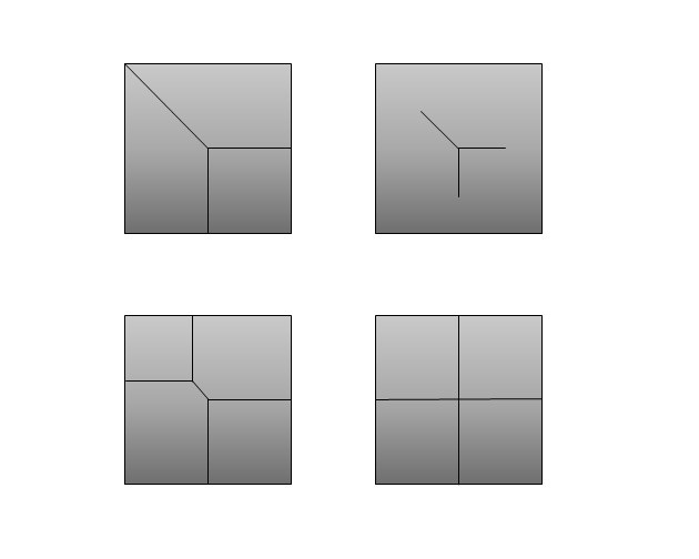
Figure 1. Top left: permissible. Top right: not permissible, since the lower-dimensional faces don’t extend to the boundary. Bottom left: permissible. Bottom Right: not permissible, since the mixed-dimensional and equidimensional indexing don’t match.

There are a few limitations to the embedding we describe in section 3 which are worth highlighting. The most significant limitation is that we do not account for mixed-dimensional geometries where lower-dimensional features do not extend towards the outer boundary. A second limitation is that we do not consider geometries where the index sets are not matching, e.g. higher degree of intersections. In fig. 1, we present two geometries which falls under these two limitations, and two geometries which are allowed, despite being similar to their non-permissible counterpart. We do not believe either of the restrictions mentioned here are indispensable, but imposing them simplifies the exposition considerably.

2.6. Differences between the Čech- and simplicial de Rham complexes

The two cochain complexes we consider are similar in several ways. They both consist of differential forms in a product space with a hierarchy of codimension/degree of overlap. Under our stated assumptions, we can index the hierarchies by the same index set $\mathcal{I}$. The 1-1 correspondence also is assumed to hold for the corresponding multi-indices. Both cochain complexes have the exterior derivative as one of the differential operators, and the jump/difference operator increases the degree $p$ of codimension/degree of overlap. One of the differences between the cochain complexes is their lengths. If the maximal degree of a differential form on a submanifold exceeds the dimension of the submanifold, the differential form is evaluated to zero. Therefore, non-trivial differential forms on the simplicial de Rham complex has maximal degree $n-p$, where $p$ is the codimension of the simplex it is defined on. On the other hand, the Čech-de Rham complex is equidimensional, and we can therefore have non-trivial differential forms of degree $n$ on intersections of degree $p$.

As a consequence, the bigrades of the double complexes are not matching. The Čech-de Rham complex is defined for each $\mathcal{A}^{p,q}$ with $p\in\{0,...,n\}$ and $q\in\{0,...,n\}$. On the other hand, the simplicial de Rham complex is only defined for $\mathcal{S}^{p,q}$ satisfying $0\leq p+q\leq n$. Thus the simplicial de Rham complex is triangular in shape, while the Čech-de Rham is rectangular in shape. The total complex of the Čech-de Rham complex is of length $2n$, but the the total simplicial de Rham complex has always length $n$:

(2.24)

Since the cochain complexes are not matching, in order for us to have a cochain map we require that the top cochain map $\Xi^{n}$ is a mapping to the kernel of $\mathcal{A}^{n}$, e.g. $\Xi^{n}:\mathcal{S}^{n}\to\ker(D^{n})$. Equivalently, we can say that we are constructing a cochain map to the truncated Čech-de Rham complex, which is the subcomplex

$$0\to\mathcal{A}^{0}\to...\to\mathcal{A}^{n-1}\to\ker(D^{n})\to 0.$$ (2.25)

By abuse of notation, we write $\mathcal{A}^{n}$ for the last part of the truncated complex and simply refer to it as the Čech-de Rham complex.

3. Constructing cochain maps

We now address the main goal of this paper, which is to construct an injective bigraded cochain map from the simplicial de Rham complex to the Čech-de Rham complex. More specifically, we are looking at the Sobolev simplicial de Rham complex with enhanced boundary regularity and where outer lower-dimensional simplices are ignored, and the truncated Čech-de Rham complex, also with Sobolev coefficients.

Although we are considering the simplicial de Rham complex, a larger class of mixed-dimensional geometries can be represented by bijectively mapping the more general mixed-dimensional geometry to the simplicial geometry.

3.1. Notation

We let $\{\Omega_{i}\}_{i\in\mathcal{I}}$ denote a given simplicial complex, and let $\mathcal{U}=\{U_{i}\}_{i\in\mathcal{I}}$ be the associated open cover, indexed by the same set $\mathcal{I}$. The construction of this open cover is described later in section 3.3. The simplicial de Rham complex is written as $(\mathcal{S}^{\bullet,\bullet},d_{\mathcal{S}},\delta_{\mathcal{S}})$, and the Čech-de Rham complex is written as $(\mathcal{A}^{\bullet,\bullet},d_{\mathcal{A}},\delta_{\mathcal{A}})$.

We write $\Xi$ for the cochain map between the double complexes, with components $\Xi^{p,q}:\mathcal{S}^{p,q}\to\mathcal{A}^{p,q}$ for ${p,q\geq 0}$.

(3.1)

By assumption, for each $\Omega_{i}$, there is a corresponding open set $U_{i}$. The intersection $U_{i}\cap U_{j}$ corresponds to $\Omega_{i,j}$, which is the common boundary of $\Omega_{i}$ and $\Omega_{j}$. We define $\tilde{U}_{i}\subset U_{i}$ to be the part of $U_{i}$ which does not intersect with any of the other open sets $U_{j}$, $j\in\mathcal{I}$. More precisely, for $i\in\mathcal{I}^{p}$, we define $\tilde{U}_{i}$ as follows:

$$\tilde{U}_{i}=U_{i}\setminus\{\bigcup_{j\in\mathcal{I}^{p},j\neq i}\overline{U_{j}}\},\qquad i\in\mathcal{I}^{p}.$$ (3.2)

We then consider for each $p$ and $i\in\mathcal{I}^{p}$, a transformation $\phi_{i}:\tilde{U}_{i}\to\Omega_{i}$. Each of the maps $\phi_{i}$ induces a pullback on differential forms: $\phi_{i}^{*}:H\Lambda^{\bullet}(\Omega_{i},\mathrm{tr})\to H\Lambda^{\bullet}(\tilde{U}_{i})$. An example of one of these pullbacks is illustrated in fig. 2. Our goal now is to extend the map $\phi_{i}^{*}:H\Lambda^{\bullet}(\Omega_{i},\mathrm{tr})\to H\Lambda^{\bullet}(\tilde{U}_{i})$ to a map which has codomain $H\Lambda^{\bullet}({U}_{i})$.

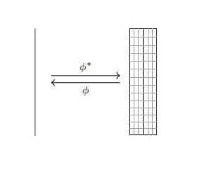
Figure 2. On the left, we have a one-dimensional manifold $\Omega_{i}$ with codimension one. On the right, we have the corresponding $\tilde{U}_{i}$. $\Omega_{i}$ is a submanifold of $\tilde{U}_{i}$, and $\phi$ is the restriction onto $\Omega_{i}$. The induced pullback is then a mapping of differential forms from $\Omega_{i}$ onto $\tilde{U}_{i}$, where the differential forms are constant along the lines normal to $\Omega_{i}$.

3.2. Example in $2D$

We consider the 2-dimensional mixed-dimensional geometry consisting of three domains $\Omega_{0},\Omega_{1},\Omega_{2}$, three interfaces $\Omega_{0,1},\Omega_{0,2},\Omega_{1,2}$ and an intersecting point $\Omega_{0,1,2}$, as illustrated in fig. 3.

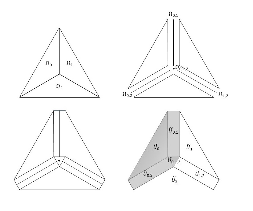
Figure 3. Top left: a simplicial geometry with three adjacent triangles. Top right: the mixed-dimensional decomposition, consisting of the three triangles, the three pairwise shared edges and a vertex in the center. Bottom left: the edges are stretched out in their tangent direction. Bottom right: the open set $U_{0}$ is highlighted in grey.

For our example geometry, we end up with a triangle in the middle covering the intersecting point $\Omega_{0,1,2}$. Each open set $U_{i}$ is then defined as the union of the original domain $\Omega_{i}$, together with the rectangles covering the interfaces $\Omega_{i,j}$ and the triangle covering $\Omega_{0,1,2}$.

For the example in question, we have the following diagram of cochain maps between the two complexes:

(3.3)

That is, we need to construct cochain maps $\Xi^{0}$, $\Xi^{1}=\Xi^{1,0}\oplus\Xi^{0,1}$ and $\Xi^{2}=\Xi^{2,0}\oplus\Xi^{1,1}\oplus\Xi^{0,2}$. For $p=0$, we have 3 domains, for $p=1$ we also have 3 domains, and for $p=2$ we have 1 domain in both the mixed-dimensional and equidimensional case. We write $f=(f_{0},f_{1},f_{2})$ for functions $f_{i}$ with domains $\Omega_{i}$, $g=(g_{0,1},g_{0,2},g_{1,2})$ for functions $g_{i,j}$ with domains $\Omega_{i,j}$ and $c$ for a constant on $\Omega_{0,1,2}$. For differential forms with degree $q>0$, we write $\alpha=(\alpha_{0},\alpha_{1},\alpha_{2})$ for differential 1-forms $\alpha_{i}$ with domains $\Omega_{i}$, $\beta=(\beta_{0,1},\beta_{0,2},\beta_{1,2})$ for differential 1-forms $\beta_{i,j}$ with domains $\Omega_{i,j}$ and $\omega=(\omega_{0},\omega_{1},\omega_{2})$ for differential 2-forms $\omega_{i}$ with domains $\Omega_{i}$. We make use of the pullbacks $\phi^{*}_{i}:H\Lambda^{\bullet}(\Omega_{i},\mathrm{tr})\to H\Lambda^{\bullet}(\tilde{U}_{i})$, for each $i\in\mathcal{I}^{p}$, the trace operator $\mathrm{tr}_{i,j}:H\Lambda^{\bullet}(\Omega_{i},\mathrm{tr})\to H\Lambda^{\bullet}(\Omega_{i,j},\mathrm{tr})$, as well as the iterated trace $\mathrm{tr}^{2}:H\Lambda^{\bullet}(\Omega_{i},\mathrm{tr})\to H\Lambda^{\bullet}(\Omega_{0,1,2},\mathrm{tr})$ to construct the cochain maps.

Consider the following cochain map for functions on the top level domains:

$$\Xi^{0,0}(f)_{i}=\begin{cases}\phi^{*}_{i}(f_{i})\qquad&\text{on}\;\tilde{U}_{i},\\ \phi_{i,j}^{*}(\mathrm{tr}\;f_{i})\qquad&\text{on}\;\tilde{U}_{i,j},\\ \phi_{0,1,2}^{*}(\mathrm{tr}^{2}\;f_{i})\qquad&\text{on}\;\tilde{U}_{0,1,2}.\end{cases}$$ (3.4)

The function $\Xi^{0,0}(f)_{i}\in\Lambda^{0}(U_{i})$, and $\tilde{U}_{i}$, $\tilde{U}_{i,j}$ and $\tilde{U}_{0,1,2}$ are understood as subsets of $U_{i}$ and note that $\tilde{U}_{0,1,2}=U_{0,1,2}$. The map $\phi_{i,j}^{*}(\mathrm{tr}\;f_{i})$ takes the boundary values of the function $f_{i}\in H\Lambda^{0}(\Omega_{i},\mathrm{tr})$ and maps it to the domain $\Omega_{i,j}$. The boundary data is then mapped to $U_{i,j}$, extended constantly in the direction which is normal to $\Omega_{i,j}$.

The next cochain map is $\Xi^{1}=\Xi^{1,0}\oplus\Xi^{0,1}$. For functions on the interfaces $\Omega_{i,j}$, we have the following cochain map:

$$\Xi^{1,0}(g)_{i,j}=\begin{cases}\phi_{i,j}^{*}(g_{i,j})\qquad&\text{on}\;\tilde{U}_{i,j},\\ \phi_{0,1,2}^{*}(\mathrm{tr}\;g_{i,j})\qquad&\text{on}\;\tilde{U}_{0,1,2}.\end{cases}$$ (3.5)

The cochain map $\Xi^{0,1}$ is similar to $\Xi^{0,0}$, except we are considering the pullback of differential forms of degree $1$:

$$\Xi^{0,1}(\alpha)_{i}=\begin{cases}\phi^{*}_{i}(\alpha_{i})\qquad&\text{on}\;\tilde{U}_{i},\\ \phi_{i,j}^{*}(\mathrm{tr}\;\alpha_{i})\qquad&\text{on}\;\tilde{U}_{i,j},\\ 0\qquad&\text{on}\;\tilde{U}_{0,1,2}.\end{cases}$$ (3.6)

Notice that we have $\phi_{0,1,2}^{*}(\mathrm{tr}^{2}\;\alpha_{i})=0$ because we are restricting a 1-form to a zero-dimensional tangent bundle. This is a recurring theme, that some terms with iterative traces will vanish for higher degrees of the cochain map.

For the final cochain map we have the following decomposition: $\Xi^{2}=\Xi^{2,0}\oplus\Xi^{1,1}\oplus\Xi^{0,2}$. Since $\Omega_{0,1,2}$ is a single point, we can only consider constant functions. The map $\Xi^{2,0}$ is just a constant map onto $\tilde{U}_{0,1,2}$:

$$\Xi^{2,0}(c)=\phi_{0,1,2}^{*}c=c|_{\tilde{U}_{0,1,2}}.$$ (3.7)

We have a cochain map for 1-forms on the interfaces $\Omega_{i,j}$:

$$\Xi^{1,1}(\beta)_{i,j}=\begin{cases}\phi_{i,j}^{*}(\beta_{i,j})\qquad&\text{on}\;\tilde{U}_{i,j},\\ 0\qquad&\text{on}\;\tilde{U}_{0,1,2}.\end{cases}$$ (3.8)

Following the same procedure, the 2-forms are evaluated to zero outside of $\tilde{U}_{i}$, since we are restricting a 2-form to a one/zero-dimensional tangent bundle, respectively:

$$\Xi^{0,2}(\omega)_{i}=\begin{cases}\phi^{*}_{i}\omega_{i}\qquad&\text{on}\;\tilde{U}_{i},\\ 0\qquad&\text{on}\;\tilde{U}_{i,j},\\ 0\qquad&\text{on}\;\tilde{U}_{0,1,2}.\end{cases}$$ (3.9)

We show that the image $\Xi^{p,q}(\alpha)$ is weakly differentiable and that these maps satisfies the properties of a cochain map in section 3.4.

3.3. Constructing an open cover with tubular neighborhoods

Given a simplicial complex, we want to construct an open cover for the Čech-de Rham complex. We can accomplish this by considering subsets of tubular neighborhoods of the lower-dimensional simplices.

Let $\Omega$ be an $(n-p)$-dimensional submanifold of $\mathbb{R}^{n}$, e.g. a simplex with codimension $p$. For a given $x\in\Omega$, we say that a vector $n\in T_{x}\mathbb{R}^{n}$ is normal to $\Omega$ if $\langle n,v\rangle=0$ for each $v\in T_{x}\Omega$, where $\langle\cdot,\cdot\rangle$ is the Euclidean inner product on $\mathbb{R}^{n}$. We define the normal space of $\Omega$ at $x$ to be the following vector space:

$$N_{x}\Omega=\{n\in T_{x}\mathbb{R}^{n}:\langle n,v\rangle=0,\forall v\in T_{x}\Omega\}.$$ (3.10)

The normal bundle is then the disjoint union of all the normal spaces:

$$N\Omega=\coprod_{x\in\Omega}N_{x}\Omega$$ (3.11)

One can describe the normal bundle without referring to an underlying Euclidean space, where we instead consider a Riemannian manifold $M$ with a submanifold $\Omega$, and replacing the Euclidean inner product with a Riemannian metric $g$.

Moreover, this construction can be done more generally without the use of a Riemannian metric for smooth manifold, by defining the normal bundle as the quotient bundle $N\Omega=TM|_{\Omega}/T\Omega$. This defines the topology of the normal bundle.

We define the map $E:N\Omega\to\mathbb{R}^{n}$ by

$$E(x,v)=x+v.$$ (3.12)

A tubular neighborhood of $\Omega$ is a neighborhood $U_{\Omega}\subset\mathbb{R}^{n}$ containing $\Omega$, which is diffeomorphic under $E$ to

$$V_{\Omega}=\{(x,v)\in N\Omega:|v|<\varepsilon(x)\},$$ (3.13)

where $\varepsilon:\Omega\to\mathbb{R}$ is a positive continuous function.

Theorem 3.1.

Every submanifold $\Omega$ embedded into $\mathbb{R}^{n}$ has a tubular neighborhood.

For proof of this claim, see [14, Theorem 5.2] or [15, Theorem 6.17]. This means that we assign a normal tubular neighborhood to each $(n-p)$-simplex, with $p$-dimensional normal space.

There are different ways to construct the open covers for a given simplicial geometry $\{\Omega_{i}\}_{i\in\mathcal{I}}$. One method for constructing an open cover is to assign a normal tubular neighborhood to each lower-dimensional simplex. Subsets of these tubular neighborhoods are chosen in such a way that they glue together to a simply-connected open set $U_{i}$.

Another construction is to consider the open set as everything which is $\varepsilon$-close to $\Omega_{i}$. For each $n$-simplex $\Omega_{i}$, we take a ball with radius $\varepsilon$ centered at each point on the boundary $x\in\partial\Omega_{i}$. We define $U_{i}$ to be the union of $\Omega_{i}$ and each of the open balls:

$$U_{i}=\Omega_{i}\cup\bigcup_{x\in\partial\Omega_{i}}B(x,\varepsilon).$$ (3.14)

The two methods for constructing an open cover that are described above are shown in fig. 4.

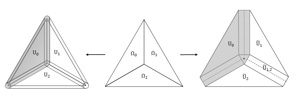
Figure 4. The figure illustrates two possible methods for constructing an open cover for a given simplicial geometry: asigning an $\varepsilon$-radius (left), or ”gluing” together subsets of tubular neighborhoods (right).

The following summarizes the assumption we put on the open cover $\mathcal{U}$:

• The indexing of the open cover $\mathcal{U}=\{U_{i}\}_{i\in\mathcal{I}}$ corresponds one-to-one with the indexing of $\{\Omega_{i}\}_{i\in\mathcal{I}}$.

• Each intersection $U_{i_{0},...,i_{p}}$ corresponds to a $(n-p)$-simplex $\Omega_{i_{0},...,i_{p}}$.

• The intersections $U_{i_{0},...,i_{p}}$ have a well-defined tangential direction and normal direction, as well as a positive distance function $\varepsilon_{i}$.

• For $i\in\mathcal{I}^{p}$, we have that $\partial\tilde{U}_{i}\cap\partial\tilde{U}_{j}$ has measure zero for all $j\in\mathcal{I}^{p+s}$, where $s\geq 2$.

The last assumption plays an important role in the next subsection, where we define the desired cochain map and show that the image of this cochain map is weakly differentiable.

3.4. The cochain maps

We now begin to describe the cochain map $\Xi^{p,q}$ locally for $i\in\mathcal{I}^{p}$. The cochain map is then obtained by assembly for each $i\in\mathcal{I}^{p}$.

We have the following formula for the cochain map:

$$\Xi^{p,q}(\alpha)_{i}=\phi_{i,j}^{*}(\mathrm{tr}^{s}\;\alpha_{i})\qquad \text{on}\;\tilde{U}_{i,j},\qquad i\in\mathcal{I}^{p},j\in\mathcal{I}^{s-1},$$ (3.15)

where $s\in\{0,...,n-p\}$, $i,j$ are disjoint and $\mathcal{I}^{-1}=\varnothing$.

We can write it explicitly for $\tilde{U}_{i}$ and each $\tilde{U}_{i,j}\subset\tilde{U}_{i}$ in the following way:

$$\Xi^{p,q}(\alpha)_{i}=\begin{cases}\phi^{*}_{i}\alpha_{i}\qquad&\text{on}\;\tilde{U}_{i},\qquad i\in\mathcal{I}^{p},\\ \vdots\\ \phi_{i,j}^{*}(\mathrm{tr}^{s}\;\alpha_{i})\qquad&\text{on}\;\tilde{U}_{i,j},\qquad i\in\mathcal{I}^{p},j\in\mathcal{I}^{s-1},\\ \vdots\\ \phi_{i,m}^{*}(\mathrm{tr}^{n-p}\;\alpha_{i})\qquad&\text{on}\;\tilde{U}_{i,m},\qquad i\in\mathcal{I}^{p},m\in\mathcal{I}^{n-p-1}.\\ \end{cases}$$ (3.16)

In order for us to prove the cochain property for $\Xi$, we first need to show that everything in the image of $\Xi$ permits a weak derivative.

Proposition 3.2.

For any $a\in\mathcal{S}^{p,q}=\prod_{i\in\mathcal{I}^{p}}H\Lambda^{q}(\Omega_{i},\mathrm{tr})$, we have that $\Xi^{p,q}(a)\in\prod_{i\in\mathcal{I}^{p}}H\Lambda^{q}(U_{i})$.

Proof.

We prove this for arbitrary fixed $p,q$ and $i\in\mathcal{I}^{p}$. We need to show that for a given $a_{i}\in H\Lambda^{q}(\Omega_{i},\mathrm{tr})$, $\alpha=\Xi^{p,q}(a_{i})$ admits a weak derivative, which we do by proving that the following integration by parts formula holds:

$$\int_{U_{i}}d\alpha\wedge\beta=(-1)^{q+1}\int_{U_{i}}\alpha\wedge d\beta,\qquad\beta\in C^{\infty}_{0}\Lambda^{n-q-1}(U_{i}).$$ (3.17)

In the expression above, $\beta$ is a smooth test-form which vanishes on the boundary of $U_{i}$, and it has degree $n-q-1$ so that $d\alpha\wedge\beta$ and $\alpha\wedge d\beta$ has degree $n$. Integration by parts and Stokes theorem gives us the following formula:

$$\int_{U_{i}}d\alpha\wedge\beta=(-1)^{q+1}\int_{U_{i}}\alpha\wedge d\beta+\int_{\partial U_{i}}\mathrm{tr}\;\alpha\wedge\mathrm{tr}\;\beta.$$ (3.18)

We write $\mathcal{I}_{i,+}=\mathcal{I}_{i}\cup\{i\}$, where $\mathcal{I}_{i}$ denotes all multi-indices containing $i$. If we show that

$$\sum_{j\in\mathcal{I}_{i,+}}\int_{\partial\tilde{U}_{j}}\mathrm{tr}\;\alpha_{j}\wedge\mathrm{tr}\;\beta_{j}=0,$$ (3.19)

then we can use the decomposition of $U_{i}$ given by eq. 3.2 to obtain the integration by parts formula:

$$\int_{U_{i}}d\alpha\wedge\beta=(-1)^{q+1}\int_{U_{i}}\alpha\wedge d\beta=(-1)^{q+1}\sum_{j\in\mathcal{I}_{i,+}}\int_{\tilde{U}_{j}}\alpha_{j}\wedge d\beta_{j}=\sum_{j\in\mathcal{I}_{i,+}}\int_{\tilde{U}_{j}}d\alpha_{j}\wedge\beta_{j}.$$ (3.20)

The first equality is the definition of weak derivative, the second equality is using the countable additivity of the Lebesgue integral, and the last equality holds if we show eq. 3.19.

We write $\Gamma_{i,j}$ for the boundary $\partial\tilde{U}_{i}\cap\partial\tilde{U}_{j}$, $j\in\mathcal{I}_{i}^{p+1}$, with orientation induced by the first index (each $\tilde{U}_{j}$ are $n$-dimensional and inherit the standard orientation from $\mathbb{R}^{n}$). The test form $\beta$ vanishes on the boundary of $U_{i}$, hence we only need to account for the boundaries of $\tilde{U}_{j}$ that are interior in $U_{i}$.

$$\int_{\partial\tilde{U}_{i}}\mathrm{tr}\;\alpha\wedge\mathrm{tr}\;\beta=\sum_{j\in\mathcal{I}_{i}^{p+1}}\int_{\Gamma_{i,j}}\mathrm{tr}\;\alpha\wedge\mathrm{tr}\;\beta.$$ (3.21)

For each integral in the right-hand side of eq. 3.21, there is a corresponding one from $\int_{\partial\tilde{U}_{j}}\mathrm{tr}\;\alpha\wedge\;\beta$ with opposite orientation due to different direction for the outward-pointing normal vector.

That is, for each integral from the boundary $\partial\tilde{U}_{i}$,

$$I_{i,j}=\int_{\Gamma_{i,j}}\mathrm{tr}\;\alpha\wedge\mathrm{tr}\;\beta=\int_{\Gamma_{i,j}}\mathrm{tr}\;\phi^{*}_{i}(a_{i})\wedge\mathrm{tr}\;\beta,$$ (3.22)

there is a corresponding integral from $\partial\tilde{U}_{j}$ with opposite orientation:

$$I_{j,i}=\int_{\Gamma_{j,i}}\mathrm{tr}\;\alpha\wedge\mathrm{tr}\;\beta=\int_{\Gamma_{j,i}}\mathrm{tr}\;\phi_{j}^{*}(\mathrm{tr}\;a_{i})\wedge\mathrm{tr}\;\beta.$$ (3.23)

By the definition of the pullback $\phi_{j}^{*}$, it extends the value of $\mathrm{tr}\;a$ constantly in the direction normal to the boundary $\Gamma_{i,j}$. The two trace operators in eq. 3.23 applies the same restriction of the tangent bundle (a projection normal to the boundary $\Gamma_{i,j}$). The integrands are therefore equal, and since the integrals have opposite orientation they cancel each other out.

More generally, we compare the integral

$$I_{l,m}=\int_{\Gamma_{l,m}}\mathrm{tr}\phi_{l}^{*}(\mathrm{tr}^{r}a_{i})\wedge\mathrm{tr}\beta$$ (3.24)

with its counterpart

$$I_{m,l}=\int_{\Gamma_{m,l}}\mathrm{tr}\phi_{m}^{*}(\mathrm{tr}^{r+1}a_{i})\wedge\mathrm{tr}\beta.$$ (3.25)

Here, $l\in\mathcal{I}^{p+r}$ and $m\in\mathcal{I}^{p+r+1}_{l}$, and the integrals $I_{l,m}$ and $I_{m,l}$ comes from $\partial\tilde{U}_{l}$ and $\partial\tilde{U}_{m}$, respectively. The expression $\phi_{m}^{*}(\mathrm{tr}^{r+1}a_{i})$ is constant in $p+r+1$ directions, including the normal direction to the boundary $\Gamma_{m,l}$. On the other hand, $\phi_{l}^{*}(\mathrm{tr}^{r}\;a_{i})$ is not constant normal to $\Gamma_{l,m}$. The two expressions inside the integrals have therefore the same codimension and are equal.

We conclude that the integrals $I_{l,m}$ and $I_{m,l}$ satisfies $I_{l,m}=-I_{m,l}$ for every $l\in\mathcal{I}^{p+r}_{i,+}$, $m\in\mathcal{I}^{p+r+1}_{l}$, and we have satisfied eq. 3.19. As a consequence, eq. 3.20 holds, and hence we have shown that the image of the cochain map permits a weak derivative. ∎

The fact that all the interior boundary integrals vanishes plays an important role in the next proposition.

Proposition 3.3.

eq. 3.15 describes an injective bigraded cochain map from the simplicial de Rham complex to the truncated Čech-de Rham complex. That is,

$$\Xi^{p,q}:\mathcal{S}^{p,q}\to\mathcal{A}^{p,q},\qquad\Xi^{p,q+1}d_{\mathcal{S}}=d_{\mathcal{A}}\Xi^{p,q},\qquad\Xi^{p+1,q}\delta_{\mathcal{S}}=\delta_{\mathcal{A}}\Xi^{p,q}.$$ (3.26)

Proof.

We let $\alpha=(\alpha_{i})_{i\in\mathcal{I}^{p}}\in\mathcal{S}^{p,q}$ be an arbitrary differential form of degree $(p,q)$. First, we want to show that the cochain map $\Xi^{p,q}$ commutes with the exterior derivative, for an arbitrary choice of $p$ and $q$. That is, $d\Xi^{p,q}(\alpha)=\Xi^{p,q+1}(d\alpha)$.

On one hand, applying the cochain map followed by the exterior derivative yields the following:

$$d\Xi^{p,q}(\alpha)_{i}=\begin{cases}d\phi^{*}_{i}\alpha_{i}\qquad&\text{on}\;\tilde{U}_{i},\qquad i\in\mathcal{I}^{p},\\ \vdots\\ d\phi_{i,j}^{*}(\mathrm{tr}^{k}\;\alpha_{i})\qquad&\text{on}\;\tilde{U}_{i,j},\qquad i\in\mathcal{I}^{p},j\in\mathcal{I}^{k-1},\\ \vdots\\ d\phi_{i,m}^{*}(\mathrm{tr}^{n-p}\;\alpha_{i})\qquad&\text{on}\;U_{i,m},\qquad i\in\mathcal{I}^{p},m\in\mathcal{I}^{n-p-1}.\\ \end{cases}$$ (3.27)

On the other hand,

$$\Xi^{p,q}(d\alpha)_{i}=\begin{cases}\phi^{*}_{i}d\alpha_{i}\qquad&\text{on}\;\tilde{U}_{i},\qquad i\in\mathcal{I}^{p},\\ \vdots\\ \phi_{i,j}^{*}(\mathrm{tr}^{k}\;d\alpha_{i})\qquad&\text{on}\;\tilde{U}_{i,j},\qquad i\in\mathcal{I}^{p},j\in\mathcal{I}^{k-1},\\ \vdots\\ \phi_{i,m}^{*}(\mathrm{tr}^{n-p}\;d\alpha_{i})\qquad&\text{on}\;U_{i,m},\qquad i\in\mathcal{I}^{p},m\in\mathcal{I}^{n-p-1}.\\ \end{cases}$$ (3.28)

We have shown in proposition 3.2 that the interior boundaries don’t contribute when we consider the decomposition of $U_{i}$. We have equality between the expressions since the exterior derivative commutes with pullbacks, and the trace operators are the pullback maps of inclusions, hence it also commutes with the exterior derivative.

Secondly, we want to show that the cochain map commutes with the difference and jump operator, i.e. that $\delta_{\mathcal{A}}\Xi^{p,q}(\alpha)=\Xi^{p+1,q}(\delta_{\mathcal{S}}\alpha)$. Recall that the difference operator is given by the following:

$$(\delta\alpha)_{i} =\sum_{l=0}^{p+1}(-1)^{k+l}\;\alpha_{i_{0},...,\hat{i}_{l},...,i_{p+1}}|_{U_{i}}, \forall i\in\mathcal{I}^{p+1}.$$ (3.29)

The jump operator $\delta_{\mathcal{S}}$ is structurally similar to the difference operator $\delta_{\mathcal{A}}$, where the dissimilarity is that we take the trace onto boundaries instead of restricting to overlaps:

$$(\delta_{\mathcal{S}}\alpha)_{i} =\sum_{l=0}^{p+1}(-1)^{k+l}\mathrm{tr}\;\alpha_{i_{0},...,\hat{i}_{l},...,i_{p+1}}, \forall i\in\mathcal{I}^{p+1}.$$ (3.30)

We let $i\in\mathcal{I}^{p+1}$ and $j\in\mathcal{I}^{s-1}$, and write $i\setminus l$ as short-hand for $(i_{0},...,\hat{i}_{l},...,i_{p+1})\in\mathcal{I}^{p}_{i}$. By applying $\Xi$ first, then the difference $\delta_{\mathcal{A}}$, we get

$$(\delta_{\mathcal{A}}\Xi^{p,q}(\alpha))_{i}=\sum_{l=0}^{p+1}(-1)^{k+l}(\Xi^{p,q}(\alpha))_{i\setminus l}|_{U_{i}}=\sum_{l=0}^{p+1}(-1)^{k+l}\phi^{*}_{i}\mathrm{tr}(\alpha_{i\setminus l}),\qquad\text{on}\;\tilde{U}_{i}.$$ (3.31)

More generally on $\tilde{U}_{i,j}$, we have

$$\delta_{\mathcal{A}}(\Xi^{p,q}(\alpha))_{i}=\sum_{l=0}^{p+1}(-1)^{k+l}\phi^{*}_{i,j}\mathrm{tr}^{s+1}(\alpha_{i\setminus l}),\qquad\text{on}\;\tilde{U}_{i,j}.$$ (3.32)

If we employ the jump operator $\delta_{\mathcal{S}}$ first, followed by the cochain map, we have the following:

$$\Xi^{p+1,q}(\delta_{\mathcal{S}}\alpha)_{i}=\phi_{(i,j)}^{*}\mathrm{tr}^{s}(\delta_{\mathcal{S}}\alpha)_{i}=\phi_{(i,j)}^{*}\mathrm{tr}^{s}\left(\sum_{l=0}^{p+1}(-1)^{k+l}\mathrm{tr}\;\alpha_{i\setminus l}\right)_{i},\qquad\text{on}\;\tilde{U}_{i,j}.$$ (3.33)

Because the pullback (and hence also the trace) is a linear operator, it commutes with the finite sum and hence we have equality between the two expressions. We therefore conclude that the cochain maps commute with the jump/difference operator.

Finally, we verify that the image of the cochain map $\Xi^{n}$ is a subset of $\ker D^{n}$. We let $\omega\in\mathcal{S}^{p,q}$ for $p+q=n$, and consider the image $\Xi^{p,q}(\omega)$. If $\omega\in\mathcal{S}^{0,n}$, then clearly the exterior derivative of $\omega$ vanishes, since we cannot have differential forms of degree $n+1$ in $n$-dimensional space. If $\omega\in\mathcal{S}^{p,q}$, with $p+q=n$ and $q<n$, then $\omega_{i}$ is a volume form on $\Omega_{i}$. Hence $\omega_{i}$ and $\Xi^{p,q}(\omega_{i})$ are $q$-forms with just one component. The differential form is extended constantly in the normal directions given by the normal tubular neighborhood, i.e. the function component of $\omega$ is constant in $p$ variables. We have the following expression for the exterior derivative of $\omega_{i}$ using local coordinates:

$$d\omega=\sum_{l=1}^{n}\frac{\partial w_{i}}{\partial x_{l}}dx_{l}\wedge dx_{i}.$$ (3.34)

For each $l\in\{1,...,n\}$, either the partial derivative $\frac{\partial w_{i}}{\partial x_{l}}$ is zero because $w_{i}$ is constant in the normal direction, or the covector $dx_{l}$ is already in $dx_{i}$. Each summand is therefore zero, and hence the exterior derivative of any differential form in the image of $\Xi^{n}$ must be zero.

We also require that everything in the image $\Xi^{n}(\omega)$ is mapped to zero by the difference operator $\delta_{\mathcal{A}}$. For $\omega\in\mathcal{S}^{p,q}$, the extension $\Xi^{p,q}(\omega)_{i}$ is nonzero only on $\tilde{U}_{i}$, and vanishes on overlaps of higher degree:

$$\Xi^{p,q}(\omega)_{i}=\begin{cases}\phi^{*}_{i}\omega_{i}\qquad&\text{on}\;\tilde{U}_{i},\qquad i\in\mathcal{I}^{p},\\ \vdots\\ \phi_{i,j}^{*}(\mathrm{tr}^{k}\;\omega_{i})=0\qquad&\text{on}\;\tilde{U}_{i,j},\qquad i\in\mathcal{I}^{p},j\in\mathcal{I}^{k-1},\\ \vdots\\ \phi_{i,m}^{*}(\mathrm{tr}^{n-p}\;\omega_{i})=0\qquad&\text{on}\;U_{i,m},\qquad i\in\mathcal{I}^{p},m\in\mathcal{I}^{n-p-1}.\\ \end{cases}$$ (3.35)

Since $\omega_{i}$ is a volume form on $\Omega_{i}$, its trace is zero, and hence $\Xi^{n}(\omega)_{i}$ is only nonzero on $\tilde{U}_{i}$. When we apply $\delta_{\mathcal{A}}$ we get that each $\Xi^{n}(\omega)_{i}$ is zero on overlaps, and hence the image of $\delta_{\mathcal{A}}^{n}$ is zero. We therefore conclude that the cochain map described is compatible with the truncation of the Čech-de Rham complex.

We have shown that the cochain maps in eq. 3.15 commute with the exterior derivative, commute with the jump/difference operators and that the image of the last cochain map $\Xi^{n}$ is in $\ker D^{n}$. ∎

4. Boundedness of the cochain map

We have in the previous section defined a cochain map from the simplicial de Rham complex to the Čech-de Rham complex, and we continue in this section by proving that $\Xi$ is bounded from both above and below. In order to do so we need to introduce the various norms associated with the two complexes. Since we are working with Hilbert complexes, each Hilbert complex has an associated inner product, and the associated inner product induces a norm $\|\alpha\|=\langle\alpha,\alpha\rangle_{C^{k}}^{1/2}$.

Recall that a graph norm of a cochain complex is defined as follows:

$$\|\alpha\|_{D}^{2}=\|\alpha\|^{2}+\|D\alpha\|^{2},$$ (4.1)

where we have omitted the subscript for the $L^{2}$ norms. Locally, the graph norm of the simplicial de Rham complex takes the following form:

$$\|\alpha_{i}\|_{\mathcal{S}^{p,q}_{i}}^{2}=\|\alpha_{i}\|^{2}+\|d\alpha_{i}\|^{2}+\sum_{j\in\mathcal{I}_{i}}\|\mathrm{tr}_{j}\alpha_{i}\|^{2}_{\mathcal{S}^{p+1,q}_{j}}.$$ (4.2)

The graph norm of the simplicial de Rham complex is the sum of the local norm defined above. We define a local graph norm for the Čech-de Rham complex to have the same recursive form as eq. 4.2:

$$\|\beta_{i}\|_{\mathcal{A}^{p,q}_{i}}^{2}=\|\beta_{i}\|^{2}+\|d\beta_{i}\|^{2}+\sum_{j\in\mathcal{I}_{i}}\|\beta_{i}|_{U_{j}}\|^{2}_{\mathcal{A}^{p+1,q}_{j}}.$$ (4.3)

As short-hand, we use subscripts $\mathcal{S}$ and $\mathcal{A}$ for the graph norms of the two double complexes and omit the indices.

Proposition 4.1.

$\Xi^{p,q}$ is a bounded cochain map, meaning there exists a constant $C_{1}$ such that

$$\|\Xi^{p,q}(\alpha)\|_{\mathcal{A}}\leq C_{1}\|\alpha\|_{\mathcal{S}},\qquad\forall\alpha\in\mathcal{S}^{p,q}.$$ (4.4)

Proof.

We consider the problem for a given component $\alpha_{i}$, $i\in\mathcal{I}^{p}$. If we show that

$$\|\Xi^{p,q}(\alpha_{i})\|_{\mathcal{A}}\leq C_{1}\|\alpha_{i}\|_{\mathcal{S}},\qquad\forall\alpha_{i}\in H\Lambda^{q}(\Omega_{i},\mathrm{tr}),$$ (4.5)

then the inequality in eq. 4.4 follows because we have a 1-1 correspondence between the domains $\Omega_{i}$ and $\tilde{U}_{i}$. Using the definition of $\Xi^{p,q}$, we split $\|\Xi^{p,q}(\alpha_{i})\|_{\mathcal{A}}$ further into the different components of the map $\Xi^{p,q}$:

$$\|\Xi^{p,q}(\alpha_{i})\|_{\mathcal{A}}=\|\phi_{i}^{*}\alpha_{i}\|_{\mathcal{A}}+\sum_{j\in\mathcal{I}_{i}}\|\phi^{*}_{j}\mathrm{tr}^{s}\alpha_{i}\|_{\mathcal{A}}.$$ (4.6)

Splitting $\|\Xi^{p,q}(\alpha_{i})\|_{\mathcal{A}}$ into the sum of norms works because of proposition 3.2. From the constructions detailed in section 3.3, we assume that each $U_{j}$ is contained in an $\varepsilon$-tubular neighborhood of $\Omega_{j}$. Since the pullbacks are constant in the normal directions, each pullback is bounded by the length $\varepsilon_{j}$:

$$c(\varepsilon_{j})\|\alpha_{i}\|_{\mathcal{S}}\leq\|\phi_{j}^{*}\alpha_{i}\|_{\mathcal{A}}\leq C(\varepsilon_{j})\|\alpha_{i}\|_{\mathcal{S}},$$ (4.7)

We therefore have

$$\|\Xi^{p,q}(\alpha_{i})\|_{\mathcal{A}} =\|\phi_{i}^{*}\alpha_{i}\|_{\mathcal{A}}+\sum_{j\in\mathcal{I}_{i}}\|\phi^{*}_{j}\mathrm{tr}^{s}\alpha_{i}\|_{\mathcal{A}}$$ (4.8)

$$\leq C(\varepsilon_{i})\|\alpha_{i}\|_{\mathcal{S}}+\sum_{j\in\mathcal{I}_{i}}C(\varepsilon_{j})\|\mathrm{tr}^{s}_{j}\alpha_{i}\|_{\mathcal{S}}.$$ (4.9)

Next, we make use of the norm in eq. 4.2. The term $\|\mathrm{tr}_{j}^{s}\alpha_{i}\|_{\mathcal{S}}$ is contained in the definition of the norm $\|\alpha_{i}\|_{\mathcal{S}}$ due to its recursive definition, hence we have a bound:

$$\|\mathrm{tr}_{j}^{s}\alpha_{i}\|_{\mathcal{S}}\leq\|\alpha_{i}\|_{\mathcal{S}}.$$ (4.10)

Putting it all together, we have the following estimate:

$$\|\Xi^{p,q}(\alpha_{i})\|_{\mathcal{A}} =\|\phi_{i}^{*}\alpha_{i}\|_{\mathcal{A}}+\sum_{j\in\mathcal{I}_{i}}\|\phi^{*}_{j}\mathrm{tr}^{s}_{j}\alpha_{i}\|_{\mathcal{A}}$$ (4.11)

$$\leq C(\varepsilon_{i})\|\alpha_{i}\|_{\mathcal{S}}+\sum_{j\in\mathcal{I}_{i}}C(\varepsilon_{j})\|\mathrm{tr}^{s}_{j}\alpha_{i}\|_{\mathcal{S}}$$ (4.12)

$$\leq C(\varepsilon_{i})\|\alpha_{i}\|_{\mathcal{S}}+\sum_{j\in\mathcal{I}_{i}}C(\varepsilon_{j})\|\alpha_{i}\|_{\mathcal{S}}$$ (4.13)

$$\leq(|\mathcal{I}_{i}|+1)\max_{j\in\mathcal{I}_{i}\cup\{i\}}C(\varepsilon_{j})\|\alpha_{i}\|_{\mathcal{S}}.$$ (4.14)

The final inequality is obtained by choosing the largest constant, multiplied with the number of summands plus one for the index $i$ itself. ∎

Proposition 4.2.

The cochain map $\Xi^{p,q}:\mathcal{S}^{p,q}\to\mathcal{A}^{p,q}$ is an injection, meaning that there exists a constant $C_{2}$ such that

$$\|\alpha\|_{\mathcal{S}}\leq C_{2}\|\Xi^{p,q}(\alpha)\|_{\mathcal{A}},\qquad\forall\alpha\in\mathcal{S}^{p,q}.$$ (4.15)

Proof.

Again we break it down for a single component, as the result stated in the proposition then immediately follows. On the left-hand side we have $\|\alpha_{i}\|_{\mathcal{S}}$, and on the right-hand side, we have

$$\|\Xi^{p,q}(\alpha_{i})\|_{\mathcal{A}}=\|\phi_{i}^{*}\alpha_{i}\|_{\mathcal{A}}+\sum_{j\in\mathcal{I}_{i}}\|\phi_{j}^{*}\mathrm{tr}^{s}\alpha_{i}\|_{\mathcal{A}}\geq\|\phi_{i}^{*}\alpha_{i}\|_{\mathcal{A}}.$$ (4.16)

Using the boundedness of the pullbacks, we have

$$c(\varepsilon_{i})\|\alpha_{i}\|_{\mathcal{S}}\leq\|\phi_{i}^{*}\alpha_{i}\|_{\mathcal{A}}\leq\|\Xi^{p,q}(\alpha_{i})\|_{\mathcal{A}}.$$ (4.17)

∎

Remark 4.3.

We emphasize that proposition 4.1 and proposition 4.2 together imply that the cochain map is a bijection on its range, and that the range of $\Xi$ thus defines a subcomplex of $\mathcal{A}$ which is isomorphic to $\mathcal{S}$.

We may choose to define an inner product and an associated graph norm that absorbs the constants $C(\varepsilon_{i})$. The local norm in eq. 4.2 is induced by the inner product:

$$\langle\alpha_{i},\beta_{i}\rangle_{\mathcal{S}} =\langle\alpha_{i},\beta_{i}\rangle+\langle d\alpha_{i},d\beta_{i}\rangle+\sum_{j\in\mathcal{I}_{i}}\langle\mathrm{tr}_{j}\alpha_{i},\mathrm{tr}_{j}\beta_{i}\rangle_{\mathcal{S}}.$$ (4.18)

The length $C(\varepsilon_{i})$ can be added as a weight to the inner product

$$\langle\alpha_{i},\beta_{i}\rangle_{\mathcal{S},\varepsilon_{i}}=\langle C(\varepsilon_{i})^{2}\alpha_{i},\beta_{i}\rangle_{\mathcal{S}}.$$ (4.19)

For constant weights $C(\varepsilon_{i})$, the associated weighted norm is given:

$$\|\alpha_{i}\|_{\mathcal{S},\varepsilon_{i}}=C(\varepsilon_{i})\|\alpha_{i}\|_{\mathcal{S}}.$$ (4.20)

From eq. 4.12, we have the following:

$$C(\varepsilon_{i})\|\alpha_{i}\|_{\mathcal{S}}+\sum_{j\in\mathcal{I}_{i}}C(\varepsilon_{j})\|\mathrm{tr}^{s}_{j}\alpha_{i}\|_{\mathcal{S}}=\|\alpha_{i}\|_{\mathcal{S},\varepsilon_{i}}+\sum_{j\in\mathcal{I}_{i}}\|\mathrm{tr}^{s}_{j}\alpha_{i}\|_{\mathcal{S},\varepsilon_{j}}.$$ (4.21)

Following the same arguments as in proposition 4.1, we obtain a proof which is independent of choice of $\varepsilon_{i}$ for the open cover.

5. Summary

We consider a simplicial geometry and construct an associated open cover with a matching index set $\mathcal{I}$, where each lower-dimensional manifold $\Omega_{j}$ is given a thickness $\varepsilon_{j}$ and corresponds to the overlap $U_{j}=U_{j_{0}}\cap...\cap U_{j_{p}}$. We define the Hilbert simplicial-de Rham complex for the simplicial geometry and the Hilbert Čech-de Rham complex for the open cover. By considering the correct subscomplexes of the simplicial de Rham complex and the Čech-de Rham complex, we are able to construct an injective cochain map between the two complexes. An explicit formula for the cochain map is expressed in eq. 3.15.

As a consequence, we can realize the simplicial de Rham complex as a subcomplex of the Čech-de Rham complex. This embedding plays an important role in comparing mixed-dimensional models with their equidimensional equivalent models. Concretely, since the image of the cochain map is a subcomplex of the Čech-de Rham complex, the complex $\mathcal{A}^{\bullet}$ becomes an appropriate setting for considering an approximation theory between mixed-dimensional and equidimensional models of compatible physical phenomena.

References

- [1] Paolo Aluffi. Algebra: chapter 0, volume 104. American Mathematical Soc., 2021.
- [2] Douglas N. Arnold, Richard S. Falk, and Ragnar Winther. Defferential complexes and stability of finite element methods ii: The elasticity complex. In Douglas N. Arnold, Pavel B. Bochev, Richard B. Lehoucq, Roy A. Nicolaides, and Mikhail Shashkov, editors, Compatible Spatial Discretizations, pages 47–67, 2006.
- [3] Douglas N Arnold, Richard S Falk, and Ragnar Winther. Finite element exterior calculus, homological techniques, and applications. Acta numerica, 15:1–155, 2006.
- [4] Douglas N Arnold, Richard S Falk, and Ragnar Winther. Finite element exterior calculus: from hodge theory to numerical stability. Bulletin of the American mathematical society, 47(2):281–354, 2010.
- [5] Wietse M Boon, Daniel F Holmen, Jan M Nordbotten, and Jon E Vatne. The Hodge-Laplacian on the Čech-de Rham complex governs coupled problems. arXiv preprint arXiv:2211.04556, 2022.
- [6] Wietse M Boon and Jan M Nordbotten. Mixed-dimensional poromechanical models of fractured porous media. Acta Mechanica, 234(3):1121–1168, 2023.
- [7] Wietse M Boon, Jan M Nordbotten, and Jon E Vatne. Functional analysis and exterior calculus on mixed-dimensional geometries. Annali di Matematica Pura ed Applicata (1923-), 200(2):757–789, 2021.
- [8] Raoul Bott and Loring W Tu. Differential forms in algebraic topology, volume 82. Springer, 1982.
- [9] John R Brauer and BS Brown. Mixed-dimensional finite-element models of electromagnetic coupling and shielding. IEEE transactions on electromagnetic compatibility, 35(2):235–241, 1993.
- [10] Annalisa Buffa and Snorre H Christiansen. The electric field integral equation on lipschitz screens: definitions and numerical approximation. Numerische Mathematik, 94:229–267, 2003.
- [11] Georges A Deschamps. Electromagnetics and differential forms. Proceedings of the IEEE, 69(6):676–696, 1981.
- [12] Richard S. Falk and Michael Neilan. Stokes complexes and the construction of stable finite elements with pointwise mass conservation. SIAM Journal on Numerical Analysis, 51(2):1308–1326, 2013.
- [13] Richard S Falk and Ragnar Winther. Double complexes and local cochain projections. Numerical methods for partial differential equations, 31(2):541–551, 2015.
- [14] Morris W Hirsch. Differential topology, volume 33. Springer Science & Business Media, 2012.
- [15] John M Lee. Smooth manifolds. Springer, 2012.
- [16] Martin W Licht. Complexes of discrete distributional differential forms and their homology theory. Foundations of Computational Mathematics, 17(4):1085–1122, 2017.
- [17] Dirk Pauly and Walter Zulehner. The elasticity complex: compact embeddings and regular decompositions. Applicable Analysis, 102(16):4393–4421, 2023.