Einstein-Podolsky-Rosen correlations in spontaneous parametric down-conversion:
Beyond the gaussian approximation

Abstract

We present analytic expressions for the coincidence detection probability amplitudes of photon pairs generated by spontaneous parametric down-conversion in both momentum and position spaces, without making use of the Gaussian approximation, and taking into account the effects of birefringence in the nonlinear crystal. We also present experimental data supporting our theoretical predictions, using Einstein-Podolsky-Rosen correlations as benchmarks, for 8 different pump beam configurations.

I Introduction

Einstein-Podolsky-Rosen (EPR) correlations in two-photon states generated by spontaneous parametric down-conversion (SPDC), first reported by Howell et al. [1] and by D’Angelo et al. [2], have been studied along the last two decades [3, 4, 5, 6, 7, 8, 9, 10, 11, 12]. As a rule, these works either rely on gaussian models or do not present a theoretical model for the SPDC two-photon state in both momentum and position representations to fit experimental data. A detailed discussion of Gaussian approximations in SPDC can be found in ref. [13], although in comparison with a simplified non Gaussian model, neglecting the crystal birefringence. Experimental conditions such as the pump laser beam focusing, the nonlinear crystal length and birefringence can affect EPR correlations in a way that is not explained by Gaussian models. In this work, we present a more precise theoretical model for the SPDC two-photon state in both position and momentum representations and show how well it fits experimental data.

II The two-photon state generated by SPDC

Let us consider a piece of negative birefringent nonlinear crystal (e. g., BBO) in the form of a block having its input face lying on the plane $z=0$, and cut for type I phase match with the principal plane (defined by optic axis and the pump beam propagation axis) parallel to the plane $xz$. A uv pump beam whose cross section lies entirely within the input and output faces of the crystal propagates along the $z$ axis with extraordinary ($x$) polarization. The crystal thickness in the $z$ direction is $L$.

In the k-vector (momentum) representation, the two-photon detection probability amplitude for the state generated by SPDC in the paraxial approximation is known to be well described (up to a normalization constant) by [14]

$$\psi({\bm{\mathrm{q}}}_{1},{\bm{\mathrm{q}}}_{2}) =\mathcal{E}_{0}({\bm{\mathrm{q}}}_{1}+{\bm{\mathrm{q}}}_{2})e^{-i\Delta_{oo}}\operatorname{sinc}\Delta_{oo},$$ (1)

where ${\bm{\mathrm{q}}}_{j}$ is the $xy$ component of ${\bm{\mathrm{k}}}_{j}$ ($j=1,2$), $\mathcal{E}_{0}({\bm{\mathrm{q}}})$ is the angular spectrum of the pump beam on the plane $z=0$,

$$\Delta_{oo}=\mu_{oo}+l_{t}(q_{1x}+q_{2x})-\frac{L}{4k_{p}}\bigg{|}\sqrt{\frac{\omega_{2}}{\omega_{1}}}{\bm{\mathrm{q}}}_{1}-\sqrt{\frac{\omega_{1}}{\omega_{2}}}{\bm{\mathrm{q}}}_{2}\bigg{|}^{2},$$

$k_{p}=\eta_{p}\omega_{p}/c$, $\omega_{p}$ is the pump laser frequency, $l_{t}$ is half of the transverse walk-off length, $\eta_{p}$ is the refractive index of the nonlinear crystal for the pump beam, $\mu_{oo}=(\bar{n}_{o}-\eta_{p})k_{p}L/2\eta_{p}$, and $\bar{n}_{o}$ is the ordinary refractive index of the nonlinear crystal at $\omega_{p}/2$. The transverse walk-off length is given by

$$2l_{t} =\frac{(n_{o}^{2}-n_{e}^{2})\sin\theta\cos\theta}{n_{o}^{2}\sin^{2}\theta+n_{e}^{2}\cos^{2}\theta}L,$$ (2)

where $n_{o}$ and $n_{e}$ are the ordinary and extraordinary refractive indices, respectively, at $\omega_{p}$, and $\theta$ is the angle between the optic axis and the pump beam propagation direction ($z$).

Here we work in the collinear phase match condition, where $\bar{n}_{o}=\eta_{p}\rightarrow\mu_{oo}=0$, and in the quasi-degenerate regime, where $\omega_{1}=(1+\nu)\omega_{p}/2$ and $\omega_{2}=(1-\nu)\omega_{p}/2$, with $\nu\ll 1$. This means that $\sqrt{\omega_{2}/\omega_{1}}\approx 1-\nu$ and $\sqrt{\omega_{1}/\omega_{2}}\approx 1+\nu$.

To simplify the notation, we make

$${\bm{\mathrm{Q}}} ={\bm{\mathrm{q}}}_{1}+{\bm{\mathrm{q}}}_{2},$$

$${\bm{\mathrm{P}}} =(1-\nu){\bm{\mathrm{q}}}_{1}-(1+\nu){\bm{\mathrm{q}}}_{2},$$

$$\beta^{2} =\frac{L}{4k_{p}}.$$ (3)

Then,

$$\psi({\bm{\mathrm{Q}}},{\bm{\mathrm{P}}})=\mathcal{E}_{0}({\bm{\mathrm{Q}}})\operatorname{sinc}(l_{t}Q_{x}-\beta^{2}P^{2})e^{-i(l_{t}Q_{x}-\beta^{2}P^{2})}.$$ (4)

On the output face of the nonlinear crystal, at $z=L$, the propagated $\psi({\bm{\mathrm{Q}}},{\bm{\mathrm{P}}})$ is

$$\psi({\bm{\mathrm{Q}}},{\bm{\mathrm{P}}},L) =\psi({\bm{\mathrm{Q}}},{\bm{\mathrm{P}}})e^{i(k_{1z}+k_{2z})L}.$$ (5)

Inside the crystal, in the collinear phase match [14],

$$(k_{1z}+k_{2z})L =\frac{\bar{n}_{o}L}{c}(\omega_{1}+\omega_{2})$$

$$-\frac{Lc}{\bar{n}_{o}}[(1-\nu)q_{1}^{2}+(1+\nu)q_{2}^{2}]$$

$$=k_{p}L-2\beta^{2}(Q^{2}+P^{2}).$$ (6)

Therefore,

$$\psi({\bm{\mathrm{Q}}},{\bm{\mathrm{P}}},L) =\mathcal{E}_{0}({\bm{\mathrm{Q}}})\operatorname{sinc}(l_{t}Q_{x}-\beta^{2}P^{2})$$

$$\times e^{-i(l_{t}Q_{x}+2\beta^{2}Q^{2})}e^{-i\beta^{2}P^{2}}.$$ (7)

Considering a Gaussian pump beam, we can write, in the complex notation [15],

$$\mathcal{E}({\bm{\mathrm{Q}}},z)=A\,e^{ik^{v}_{p}z}e^{-ia(z)Q^{2}/2k^{v}_{p}},$$ (8)

where $A$ is a constant, $k^{v}_{p}=\omega_{p}/c$ (superscript $v$ stands for vacuum), $a(z)=z-z_{c}-ik^{v}_{p}w_{0}^{2}/2$, $w_{0}$ is the beam waist and $z_{c}$ is the waist location on the $z$ axis. Hence,

$$\mathcal{E}_{0}({\bm{\mathrm{Q}}}) =A\,e^{-ia_{0}Q^{2}/2k^{v}_{p}},$$ (9)

where $a_{0}=a(0)$. Then, at the output face of the crystal,

$$\psi({\bm{\mathrm{Q}}},{\bm{\mathrm{P}}},L) =e^{-i(a_{0}/2k^{v}_{p}+2\beta^{2})Q^{2}}e^{-il_{t}Q_{x}}e^{-i\beta^{2}P^{2}}$$

$$\times\operatorname{sinc}(l_{t}Q_{x}-\beta^{2}P^{2}).$$ (10)

From $z=L$ to $z>L$, $\psi({\bm{\mathrm{Q}}},{\bm{\mathrm{P}}})$ propagates in free space, that is,

$$\psi({\bm{\mathrm{Q}}},{\bm{\mathrm{P}}},z)=\psi({\bm{\mathrm{Q}}},{\bm{\mathrm{P}}},L)e^{i(k^{v}_{1z}+k^{v}_{2z})(z-L)}.$$ (11)

In free space and collinear propagation,

$$(k^{v}_{1z}+k^{v}_{2z})(z-L) =\Big{(}k^{v}_{1}+k^{v}_{2}-\frac{q_{1}^{2}}{2k^{v}_{1}}-\frac{q_{2}^{2}}{2k^{v}_{2}}\Big{)}(z-L)$$

$$=k^{v}_{p}(z-L)+2\bar{n}_{o}\beta^{2}(Q^{2}+P^{2})$$

$$-\frac{z}{2k^{v}_{p}}(Q^{2}+P^{2}).$$ (12)

Therefore,

$$\psi({\bm{\mathrm{Q}}},{\bm{\mathrm{P}}},z) =\operatorname{sinc}(l_{t}Q_{x}-\beta^{2}P^{2})e^{-il_{t}Q_{x}}$$

$$\times e^{-ib_{1}(z)Q^{2}}e^{-ib_{2}(z)P^{2}},$$ (13)

where

$$b_{1}(z) =a(z)/2k^{v}_{p}-2(\bar{n}_{o}-1)\beta^{2},$$

$$b_{2}(z) =z/2k^{v}_{p}-(2\bar{n}_{o}-1)\beta^{2}.$$ (14)

To the best of our knowledge, an accurate analytic expression for $\psi$ in the coordinate representation is not available in the literature. To arrive at such expression, we adopt the following approximation: For pump beams with reasonably narrow-band angular spectra ($w_{0}\geq 50\,\mu$m) and $L\sim$ 1 mm to 5 mm, which cover most practical cases, we can make

$$\psi({\bm{\mathrm{Q}}},{\bm{\mathrm{P}}},z) =\operatorname{sinc}(l_{t}Q_{x})e^{-il_{t}Q_{x}}e^{-ib_{1}(z)Q^{2}}$$

$$\times\operatorname{sinc}(\beta^{2}P^{2})e^{-ib_{2}(z)P^{2}},$$ (15)

which turns $\psi({\bm{\mathrm{Q}}},{\bm{\mathrm{P}}},z)$ into a separable function of ${\bm{\mathrm{Q}}}$ and ${\bm{\mathrm{P}}}$. Defining the coordinates ${\bm{\mathrm{R}}}=[(1+\nu){\bm{\mathrm{\rho}}}_{1}+(1-\nu){\bm{\mathrm{\rho}}}_{2}]/2$ and ${\bm{\mathrm{S}}}=({\bm{\mathrm{\rho}}}_{1}-{\bm{\mathrm{\rho}}}_{2})/2$, the calculation of the Fourier transform of $\psi({\bm{\mathrm{Q}}},{\bm{\mathrm{P}}},z)$ is straightforward:

$$\psi({\bm{\mathrm{R}}},{\bm{\mathrm{S}}},z) =\frac{e^{-R_{y}^{2}/4ib_{1}(z)}}{l_{t}\sqrt{ib_{1}(z)}}$$

$$\times\Big{\{}\operatorname{Erf}\Big{[}\frac{R_{x}-2l_{t}}{2\sqrt{ib_{1}(z)}}\Big{]}-\operatorname{Erf}\Big{[}\frac{R_{x}}{2\sqrt{ib_{1}(z)}}\Big{]}\Big{\}}$$

$$\times\Big{\{}\operatorname{Ei}\Big{[}\frac{ik_{p}^{v}\,S^{2}}{2(z-L)}\Big{]}-\operatorname{Ei}\Big{[}\frac{ik_{p}^{v}\,S^{2}}{2(z-L^{\prime})}\Big{]}\Big{\}}$$ (16)

for $z>L$, where $L^{\prime}=(1-1/\bar{n}_{o})L$, $\operatorname{Erf}$ is the error function, and $\operatorname{Ei}$ is the exponential integral function [16].

III EPR correlations

With expressions (II) and (II) we can calculate the uncertainties $\Delta x_{1}$, $\Delta y_{1}$, for fixed $x_{2}$, $y_{2}$ and $z$, and $\Delta k_{x1}$, $\Delta k_{y1}$ for fixed $k_{x2}$, $k_{y2}$ as functions of the pump beam angular spectrum width (defined by the beam waist $w_{0}$) and see how they are affected by the crystal anisotropy (quantified here by walk-off parameter $l_{t}$). Assuming any fixed value for ${\bm{\mathrm{\rho}}}_{2}$, Eq. (II) allows us to calculate $\Delta x_{1}$ and $\Delta y_{1}$ for any $z>L$. By another side, assuming any fixed value for ${\bm{\mathrm{q}}}_{2}$, Eq. (II) allows us to calculate $\Delta k_{1x}$ and $\Delta k_{1y}$, which do not depend on $z$. As an example, Fig. 1 shows plots of $\Delta x_{1}$ and $\Delta y_{1}$ for ${\bm{\mathrm{\rho}}}_{2}=0$ and plots of $\Delta k_{x1}$ and $\Delta k_{y1}$ for ${\bm{\mathrm{q}}}_{2}=0$, for a 5 mm-long BBO crystal pumped by 355 nm gaussian laser beams whose waists $w_{0}$ and waist positions $z_{c}$ are shown in Table 1. Uncertainties $\Delta x_{1}$ and $\Delta y_{1}$ where calculated on the plane $z=5.0001$ mm.

Table 1: Pump beam parameters.

Beam	$w_{0}$ (mm)	$z_{c}$ (mm)
1	0.062	178
2	0.067	213
3	0.072	251
4	0.085	298
5	0.095	355
6	0.105	422
7	0.120	510
8	0.142	635

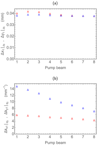
Figure 1: Predicted values of (a) $\Delta x_{1}|_{{\bm{\mathrm{\rho}}}_{2}=0}$ (red) and $\Delta y_{1}|_{{\bm{\mathrm{\rho}}}_{2}=0}$ (blue), (b) $\Delta k_{x1}|_{{\bm{\mathrm{q}}}_{2}=0}$ (red) and $\Delta k_{y1}|_{{\bm{\mathrm{q}}}_{2}=0}$ (blue) for a 5 mm-long BBO crystal pumped by 355 nm laser beams whose parameters are listed in Table 1.

One can see that while the position uncertainties in $x$ and $y$ directions are about the same, the momentum uncertainties are strongly affected by the anisotropy. This is a direct consequence of the partial transfer of the pump beam angular spectrum in the direction parallel to the principal plane [17], in our case, the $x$ direction.

It is interesting to note that the uncertainties $\Delta x_{1}$ and $\Delta y_{1}$ increase rapidly as the distance from the crystal increases in the $z$ direction. In general, position uncertainties depend on the pump beam parameters, as exemplified in Fig. 2. For a weakly focused laser beam ($w_{0}=0.5\,\mathrm{mm}$) whose waist is located at the crystal input face ($z=0$), our predictions shown in Fig. 2a are in good agreement with the results reported in Ref [11]. This agreement is due to the fact that in this case a Gaussian model fits well the uncertainty in position coordinates [13].

Figure 2: Predicted values of $\Delta x_{1}|_{{\bm{\mathrm{\rho}}}_{2}=0}$ (red) and $\Delta y_{1}|_{{\bm{\mathrm{\rho}}}_{2}=0}$ (blue) as functions of the distance from the output face of a 5 mm-long BBO crystal cut for collinear degenerate phase match, pumped by a 355 nm laser beam with (a) $w_{0}=0.5\,\mathrm{mm}$, $z_{c}=0$ and (b) $w_{0}=0.05\,\mathrm{mm}$, $z_{c}=150\,\mathrm{mm}$.

IV Experiment

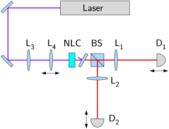
Figure 3: Experimental setup

EPR correlations predicted in the previous section were tested experimentally with the setup represented in Fig. 3. A 5 mm-long BBO crystal cut for type I collinear phase match (NLC) having its optic axis parallel to the $xz$ plane and input face located on the plane $z=0$ was pumped by a 355 nm laser beam polarized in the $x$ direction, propagating along the $z$ direction. The beam parameters, listed in Table 1, were changed with the help of a telescope composed by a lens $L_{3}$ of focal length 50 mm and a lens $L_{4}$ of focal length 40 mm separated from $L_{3}$ by a variable distance. The down-converted light, with $\lambda_{1}=690\,\mathrm{nm}$ and $\lambda_{2}=731\,\mathrm{nm}$ was sent to a beam splitter (BS) and directed to detectors $D_{1}$ (equipped with a 12 nm band-pass filter centered at 690 nm) and $D_{2}$ (equipped with a 40 nm band-pass filter centered at 730 nm). Lenses $L_{1}$ and $L_{2}$ of focal length 75 mm were placed at 150 mm from the output face of the nonlinear crystal. Detectors $D_{1}$ and $D_{2}$ were placed at 75 mm from $L_{1}$ and $L_{2}$ (Fourier plane) for the measurements of $|\psi({\bm{\mathrm{q}}}_{1},0,L)|^{2}$ and at 150 mm (1:1 image plane) for the measurements of $|\psi({\bm{\mathrm{\rho}}}_{1},0,L)|^{2}$. Each detector consists of a multimode optical fiber with diameter of $50\,\mu\mathrm{m}$, one tip mounted on a computer-controlled $xy$ motorized translation stage and the other tip coupled to a photon-counting avalanche photodiode. In all measurements, $D_{2}$ was kept at ${\bm{\mathrm{\rho}}}_{2}=0$.

Due to the relatively large fiber diameter and photon-counting fluctuations, experimental results are not directly comparable with theory. In order to check the accuracy of theoretical predictions, the following procedure was adopted: Experimental data for coincidence detections on the image plane were fit to a hyperbolic secant probability distribution $A\operatorname{sech}\pi\xi/2\sigma$ ($\xi=x,y$), whose standard deviation is given by $\sigma$. Numerical convolutions of the theoretical coincidence profiles with the 50 $\mu\mathrm{m}$ circular apertures of $D_{1}$ and $D_{2}$ were made, resulting in the expected detection probability distributions. Profiles obtained when the crystal was pumped with the laser beam #1 (see Table I) are shown in Fig. 4. An additional correction of the beam waist radius was made, due to the pump beam $M^{2}$ factor of 1.14. On the Fourier plane, a Gaussian distribution $A\exp(-\xi^{2}/2\sigma^{2})$ ($\xi=k_{x},k_{y}$) was used in a similar procedure. Experimental results and theoretical predictions are presented in Fig. 5.

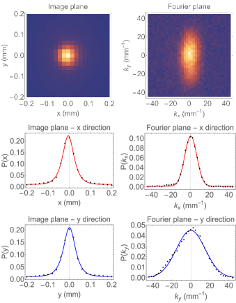
Figure 4: Top row: Examples of coincidence detection profiles on the image plane (left) and on the Fourier plane (right) for beam # 1 (see Table 1). Mid row: Corresponding detection probability densities $P(x_{1}|{\bm{\mathrm{\rho}}}_{2}=0)$ (left) and $P(y_{1}|{\bm{\mathrm{\rho}}}_{2}=0)$ (right). Bottom row: Corresponding detection probability densities $P(k_{x1}|{\bm{\mathrm{q}}}_{2}=0)$ (left) and $P(k_{y1}|{\bm{\mathrm{q}}}_{2}=0)$ (right). Dots are normalized experimental data and solid lines are best fits for distributions $A\operatorname{sech}\pi\xi/2\sigma$ ($\xi=x,y$ on the image plane) and $A\exp(-\xi^{2}/2\sigma^{2})$ ($\xi=k_{x},k_{y}$ on the Fourier plane).

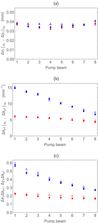
Figure 5: Measured ($\bullet$) and predicted ($\triangle$) values of (a) $\Delta x_{1}$ (red) and $\Delta y_{1}$ (blue), (b) $\Delta k_{x1}$ (red) and $\Delta k_{y1}$ (blue), (c) $\Delta x_{1}\Delta k_{x1}$ (red) and $\Delta y_{1}\Delta k_{y1}$ (blue) for a 5 mm-long BBO crystal pumped by 355 nm laser beams whose parameters are listed in Table 1.

V Discussion and Conclusion

From the results presented here, one can see that the EPR correlations $\Delta x\Delta k_{x}$ and $\Delta y\Delta k_{y}$ of the photons pairs generated by spontaneous parametric down-conversion are strongly affected by the pump beam angular spectrum in the direction normal to the principal plane (defined by the optic axis and the $z$ axis). By another side, such dependence is much smaller in the direction parallel to the principal plane. This effect is readily explained by the presence of the term $\operatorname{sinc}l_{t}Q_{x}$ in Eq. (II). That term, which depends on the birefringence, on the phase match angle, and on the crystal length (see Eq. (2)), acts as a spatial filter for the transfer of the angular spectrum from the pump beam to the two-photon state [17]. Because of this filtering effect, the product $\Delta x\Delta k_{x}$ behaves as if the laser beam were less focused. The two uncertainty products $\Delta x\Delta k_{x}$ and $\Delta y\Delta k_{y}$ tend to a unique minimum value as the pump beam gets more collimated, that is, $w_{0}\gg l_{t}$. In our case, $l_{t}=0.186\,\mathrm{mm}$.

In conclusion, we have presented: (a) Accurate analytic expressions for the coincidence detection probability amplitudes of photon pairs generated by spontaneous parametric down-conversion in both momentum and position spaces. Those expressions allow us to predict how the correlations in position and momentum depend on the system parameters like crystal length, crystal birefringence, pump beam focusing, pump beam waist location and detectors location. (b) Experimental data supporting our theoretical predictions, using Einstein-Podolsky-Rosen correlations as benchmarks, for 8 different pump beam configurations.

The results presented here may be useful in any application relying on position and momentum correlations of photon pairs generated by SPDC in birefringent crystals.

References

• Howell et al. [2004] J. C. Howell, R. S. Bennink, S. J. Bentley, and R. W. Boyd, Realization of the Einstein-Podolsky-Rosen paradox using momentum- and position-entangled photons from spontaneous parametric down conversion, Phys. Rev. Lett. 92, 210403 (2004).
• D’Angelo et al. [2004] M. D’Angelo, Y.-H. Kim, S. P. Kulik, and Y. Shih, Identifying entanglement using quantum ghost interference and imaging, Phys. Rev. Lett. 92, 233601 (2004).
• Walborn et al. [2011] S. P. Walborn, A. Salles, R. M. Gomes, F. Toscano, and P. H. S. Ribeiro, Revealing hidden Einstein-Podolsky-Rosen nonlocality, Phys. Rev. Lett. 106, 130402 (2011).
• Edgar et al. [2012] M. Edgar, D. Tasca, F. Izdebski, R. Warburton, J. Leach, M. Agnew, G. Buller, R. Boyd, and M. Padgett, Imaging high-dimensional spatial entanglement with a camera, Nat. Commun. 3, 984 (2012).
• Moreau et al. [2012] P.-A. Moreau, J. Mougin-Sisini, F. Devaux, and E. Lantz, Realization of the purely spatial Einstein-Podolsky-Rosen paradox in full-field images of spontaneous parametric down-conversion, Phys. Rev. A 86, 010101 (2012).
• Moreau et al. [2014] P.-A. Moreau, F. Devaux, and E. Lantz, Einstein-Podolsky-Rosen paradox in twin images, Phys. Rev. Lett. 113, 160401 (2014).
• Schneeloch and Howland [2018] J. Schneeloch and G. A. Howland, Quantifying high-dimensional entanglement with Einstein-Podolsky-Rosen correlations, Phys. Rev. A 97, 042338 (2018).
• Chen et al. [2019] L. Chen, T. Ma, X. Qiu, D. Zhang, W. Zhang, and R. W. Boyd, Realization of the Einstein-Podolsky-Rosen paradox using radial position and radial momentum variables, Phys. Rev. Lett. 123 (2019).
• Srivastav et al. [2022] V. Srivastav, N. H. Valencia, S. Leedumrongwatthanakun, W. McCutcheon, and M. Malik, Characterizing and tailoring spatial correlations in multimode parametric down-conversion, Phys. Rev. Appl. 18, 054006 (2022).
• Bhattacharjee et al. [2022a] A. Bhattacharjee, N. Meher, and A. K. Jha, Measurement of two-photon position-momentum Einstein-Podolsky-Rosen correlations through single-photon intensity measurements, New J. Phys. 24, 053033 (2022a).
• Bhattacharjee et al. [2022b] A. Bhattacharjee, M. K. Joshi, S. Karan, J. Leach, and A. K. Jha, Propagation-induced revival of entanglement in the angle-oam bases, Sci. Adv. 8, eabn7876 (2022b).
• Patil et al. [2023] S. Patil, S. Prabhakar, A. Biswas, A. Kumar, and R. P. Singh, Anisotropic spatial entanglement, Phys. Lett. A 457, 128583 (2023).
• Gómez et al. [2012] E. S. Gómez, W. A. T. Nogueira, C. H. Monken, and G. Lima, Quantifying the non-gaussianity of the state of spatially correlated down-converted photons, Opt. Express 20, 3753 (2012).
• Walborn et al. [2010] S. P. Walborn, C. H. Monken, S. Pádua, and P. H. S. Ribeiro, Spatial correlations in parametric down-conversion, Phys. Rep. 495, 87 (2010).
• Siegman [1986] A. E. Siegman, Lasers (University Science Books, 1986).
• Lebedev [1972] N. N. Lebedev, Special Functions & Their Applications (Dover, 1972).
• da Costa Moura et al. [2010] A. G. da Costa Moura, W. A. T. Nogueira, and C. H. Monken, Fourth-order image formation by spontaneous parametric down-conversion: The effect of anisotropy, Opt. Commun. 283, 2866 (2010).