Parameter identification in PDEs by the solution of monotone inclusion problems

Abstract

In this paper we consider a parameter identification problem for a semilinear parabolic PDE. For the regularized solution of this problem, we introduce a total variation based regularization method requiring the solution of a monotone inclusion problem. We show well-posedness in the sense of inverse problems of the resulting regularization scheme. In addition, we introduce and analyze a numerical algorithm for the solution of this inclusion problem using a nested inertial primal dual method. We demonstrate by means of numerical examples the convergence of both the numerical algorithm and the regularization method.

MSC Classification] 65J20, 47H05, 47J06, 49J20

1 Introduction

Denote by $I:=[0,1]$ the unit interval, and let $\Omega\subset\mathbb{R}^{d}$, $d\in\mathbb{N}$, be a bounded domain with Lipschitz boundary. Denote by $\mathcal{A}\colon L^{2}(I\times\Omega)\to L^{2}(I\times\Omega)$ the operator that maps $u$ to the (weak) solution of the PDE

$$y_{t}+y^{3}-\Delta y =u \text{ in }I\times\Omega,$$ (1)

$$y =0 \text{ on }I\times\partial\Omega,$$

$$y(0,\cdot) =y_{0} \text{ in }\Omega.$$

Here $y_{0}\in L^{2}(\Omega)$ is some given function. We consider the inverse problem of solving the equation

$$\mathcal{A}(u)=y^{\delta},$$ (2)

given noisy data $y^{\delta}\in L^{2}(I\times\Omega)$ satisfying

$$y^{\delta}=y^{\dagger}+n^{\delta}\qquad\text{ with }\lVert n^{\delta}\rVert_{L^{2}}\leq\delta.$$

Here $y^{\dagger}=\mathcal{A}(u^{\dagger})$ is the noise free data produced from the true solution $u^{\dagger}$. That is, we want to reconstruct the source term $u^{\dagger}$ in (1) from noisy measurements of the associated solution. We stress here that we consider the case where the source $u^{\dagger}$ is both space- and time-dependent.

The problem (2) is ill-posed in that it, in general, does not have a solution in the presence of noise. Also, if a solution exists, it does not depend continuously on the right hand side. Because of that, it is necessary to apply some regularization in order to obtain a stable solution. In the literature, there exist several approaches to the regularization of this type of problems:

• In Tikhonov regularization, one computes an approximate solution of (2) by solving the minimization problem

  $$\mathcal{T}_{\alpha}(u)=\frac{1}{2}\lVert\mathcal{A}(u)-y^{\delta}\rVert_{L^{2}}^{2}+\alpha\mathcal{R}(u)\to\min.$$ (3)

  Here $\mathcal{R}\colon L^{2}(I\times\Omega)\to\mathbb{R}\cup\{+\infty\}$ is a regularization term that encodes prior information about the true solution $u^{\dagger}$, and the regularization parameter $\alpha>0$ steers the trade-off between regularity of the solution and data fidelity. See e.g. [1, 2] for an overview and analysis of this approach.

• Iterative regularization methods consider the minimization of the norm of the residual $\lVert\mathcal{A}(u)-y^{\delta}\rVert_{L^{2}}^{2}$ or a similar term by means of an iterative method. Examples are Landweber iteration (that is, gradient descent) or the iteratively regularized Gauss–Newton or Levenberg–Marquardt method. Here the regularization is performed by stopping the iteration early, well before convergence. An overview of iterative methods in a general setting can be found in [3].

• In the specific case of parameter identification problems, there are also “all-at-once” formulations, which rewrite the problem (2) as a system of equations, the first describing the equation, the second the data observation, see e.g. [4, 5].

The approach we will discuss in the following is most closely related to the Tikhonov approach. In order to motivate the method, we note that the necessary optimality condition for a solution of (3) reads

$$\mathcal{A}^{\prime}(u)^{*}\mathcal{A}(u)+\alpha\partial\mathcal{R}(u)\ni\mathcal{A}^{\prime}(u)^{*}y^{\delta},$$ (4)

provided that $\mathcal{A}$ is Fréchet differentiable and $\mathcal{R}$ is convex and lower semi-continuous with subdifferential $\partial\mathcal{R}$. If $\mathcal{A}$ is bounded linear, the necessary optimality condition is also sufficient, and the minimizer of $\mathcal{T}_{\alpha}$ is uniquely characterized by (4). In the non-linear case, however, this is in general not the case, and there may exist non-optimal solutions of (4) as well as local minimizers of $\mathcal{T}_{\alpha}$. This makes both the theoretical analysis and numerical implementation of Tikhonov regularization challenging. Iterative regularization methods based on the minimization of the residual $\lVert\mathcal{A}(u)-y^{\delta}\rVert_{L^{2}}^{2}$ face the same challenge, and most convergence and stability results for these methods hold only for initializations of the iteration sufficiently close to the true solution. In addition, the operator $\mathcal{A}$ has to satisfy additional regularity conditions, a typical example being the tangential cone condition introduced in [6, Eq. 1.5].

An alternative to Tikhonov regularization that is applicable to monotone problems is Lavrentiev regularization, see e.g. [7, 8, 9]. The classical formulation requires the solution of the monotone equation $\mathcal{A}(u)+\alpha u=y^{\delta}$. In [10], however, a generalization in the form of the monotone inclusion problem

$$\mathcal{A}(u)+\alpha\partial\mathcal{R}(u)\ni y^{\delta}$$ (5)

was proposed, which also allows for the inclusion of non-quadratic regularization terms similar to Tikhonov regularization. In contrast to (4), this inclusion problem has, under certain coercivity conditions on $\mathcal{A}$ and $\mathcal{R}$, a unique solution, and it has been shown in [10] that this leads to a stable regularization method. In this paper, we will develop this approach further and show that it can be applied to the problem (2) with a regularization term that is a combination of a total variation term in time and a squared Sobolev norm in space. Moreover, we will discuss a globally convergent solution algorithm for the numerical solution of inclusion problems of the form (5).

In the last decades, there has been a growing interest in the study of monotone inclusion problems within the fields of operator theory and computational optimization. This field of study holds significant relevance, offering practical applications in domains such as partial differential equations, and signal and image processing. The pursuit of identifying the roots of the sum of two or more maximally monotone operators within Hilbert spaces remains a dynamically evolving focus of scientific investigation [11, 12]. Notably, among the methods commonly utilized to address these challenges, splitting algorithms (see [11, Chapter 25]) have garnered significant attention.

Driven by diverse application scenarios, the research community has expressed interest in investigating primal-dual splitting algorithms to address complex structured monotone inclusion problem that encompass the presence of finitely many operators, including cases where some of these operators are combined with linear continuous operators and parallel-sum type monotone operators, see [13, 14] and the references therein. The distinguishing feature of these algorithms lies in their complete decomposability, wherein each operator is individually assessed within the algorithm, utilizing either forward or backward steps.

Primal-dual splitting algorithms, incorporating inertial effects have been featured in [15, 16, 17]. These algorithms have demonstrated clear advantages over non-inertial versions in practical experiments [15, 16]. The inertial terminology can be noticed as discretization of second order differential equations proposed by Polyak [18] to minimize a smooth convex function, the so-called heavy ball method. The presence of an inertial term provides the advantage of using the two preceding terms to determine the next iteration in the algorithm, consequently increases the convergence speed of the algorithm. Nesterov [19] modified the heavy ball method to enhance the convergence rate for smooth convex functions by using the inertial point to evaluate the gradient. In [20], Beck and Teboulle have proposed a fast iterative shrinkage-thresholding algorithm (FISTA) within the forward-backward splitting framework for the sum of two convex function, one being non-smooth. The FISTA algorithm is versatile and finds application in numerous practical problems, including sparse signal recovery, image processing, and machine learning.

In this paper, we apply non-linear Lavrentiev regularization by combining a total variation term in time and a squared Sobolev norm in space to solve the problem of the form (2). This yields a completely new, well-posed regularization method that can be extended to the solution of more general monotone ill-posed problems. We discuss the properties of the regularizers and the well-posedness of the regularization method in Section 2. In addition to showing well-posedness, we discuss the numerical solution of the regularized problem by providing a numerical algorithm using an inertial technique. There, we follow the ideas of inexact forward-backward splitting to solve the monotone inclusion problems. Section 3 provides preliminaries on $L^{2}$-valued functions of bounded variation and then provided the proof of well-posedness. We study convergence of the proposed numerical algorithm in Section 4. In Section 5, we discuss how the numerical method can be applied to the solution of our inclusion problem. Finally, in Section 6 we present some numerical experiments that show the behavior of our regularization method as well as the solution algorithm.

2 Main Results

In this paper, we make the specific assumption that the true solution $u^{\dagger}$ of (2) is a function that is smooth in the space variable, but piecewise constant in the time variable. That is, we can write

$$u^{\dagger}(x,t)=u^{\dagger}_{i}(x)\qquad\text{ if }t\in[t_{i-1},t_{i}),$$ (6)

where $0=t_{0}<t_{1}<\ldots<t_{N}=1$ is some (unknown) discretization of the unit interval, and $u_{i}^{\dagger}\in H^{1}(\Omega)$ for $i=1,\ldots,N$. Because the true solution $u^{\dagger}$ is piecewise constant in the time variable, it makes sense to apply some form of total variation regularization, which is known to promote piecewise constant solutions. However, in the spatial direction we want the solutions to be smooth, which calls for regularization with some type of Sobolev (semi-)norm. Thus we will define a regularization term that consists of the total variation only in the time variable, and an $H^{1}$-semi-norm only in the spatial variable.

Denote by

$$\mathcal{R}(u):=\operatorname{var}_{t}(u):=\sup_{\begin{subarray}{c}\varphi\in C_{0}^{1}(I;L^{2}(\Omega))\\ \lVert\varphi(t)\rVert_{L^{2}}\leq 1\text{ for all }t\in I\end{subarray}}\int_{0}^{1}\langle\varphi(t),u(t,\cdot)\rangle_{L^{2}(\Omega)}\,dt$$ (7)

the total variation of $u$ in the time variable, and by

$$\mathcal{S}(u):=\frac{1}{2}\int_{I}\lvert u(t,\cdot)\rvert_{H^{1}}^{2}\,dt=\frac{1}{2}\int_{I}\int_{\Omega}\lvert\nabla_{x}u(t,x)\rvert^{2}dx\,dt$$

the spatial $H^{1}$-semi-norm of $u$, integrated over the whole time interval $I$. We consider the solution of (2) by applying non-linear Lavrentiev regularization, consisting in the solution of the monotone operator equation

$$\mathcal{A}(u)+\partial(\lambda\mathcal{R}+\mu\mathcal{S})(u)\ni y^{\delta},$$ (8)

where $\lambda>0$ and $\mu>0$ are regularization parameters that control the temporal and spatial smoothness of the regularized solutions, respectively. Moreover, $\partial(\lambda\mathcal{R}+\mu\mathcal{S})$ is the subdifferential of the convex and lower semi-continuous function $\lambda\mathcal{R}+\mu\mathcal{S}\colon L^{2}(I\times\Omega)\to\mathbb{R}\cup\{+\infty\}$.

2.1 Well-posedness

Our first main result states that the solution of (8) is well-posed in the sense of inverse problems. That is, for all positive regularization parameters the solution exists, is unique, and depends continuously on the right hand side $y^{\delta}$. Moreover, as the noise level decreases to zero, the solution of (8) converges to the true solution of the noise free problem (2) provided the regularization parameters are chosen appropriately.

Theorem 1.

Assume that the solution $u^{\dagger}$ of the noise-free equation $\mathcal{A}(u)=y^{\dagger}$ satisfies $\mathcal{R}(u^{\dagger})+\mathcal{S}(u^{\dagger})<\infty$. The solution of (8) defines a well-posed regularization method. That is, the following hold:

• The inclusion (8) admits for each $\lambda$, $\mu>0$ and each $y^{\delta}$ a unique solution.

• Assume that $\lambda$, $\mu>0$ are fixed, and assume that $\{y_{k}\}_{k\in\mathbb{N}}\in L^{2}(I\times\Omega)$ converge to some $y\in L^{2}(I\times\Omega)$. Denote moreover by $u_{k}$ and $u$ the solutions of (8) with right hand sides $y_{k}$ and $y$, respectively. If $\lVert y_{k}-y\rVert_{L^{2}}\to 0$, then also $\lVert u_{k}-u\rVert_{L^{2}}\to 0$.

• Assume that $\lambda=\lambda(\delta)$ and $\mu=\mu(\delta)$ are chosen such that

  $$\lambda(\delta),\ \mu(\delta)\to 0,\qquad\text{ and }\qquad\frac{\delta}{\lambda(\delta)},\ \frac{\delta}{\mu(\delta)}\qquad\text{ are bounded as }\delta\to 0.$$

  Denote by $u^{\delta}_{\lambda,\mu}=u^{\delta}_{\lambda(\delta),\mu(\delta)}$ the solution of (8) with right hand side $y^{\delta}$ satisfying $\lVert y^{\delta}-y^{\dagger}\rVert_{L^{2}}\leq\delta$. Then $\lVert u^{\delta}_{\lambda,\mu}-u^{\dagger}\rVert_{L^{2}}\to 0$ as $\delta\to 0$.

The proof of this result can be found in Section 3.2 below. It mainly relies on a recent general result concerning non-linear Lavrentiev regularization [10]. In addition, we rely on certain properties of functions of bounded variations with values in a Banach or Hilbert space, see [21]. The main results on functions of bounded variation that we need are collected in Section 3.1.

We now discuss the numerical solution of (8). First, we note that the domains of both $\mathcal{R}$ and $\mathcal{S}$ are dense proper subspaces of $L^{2}(I\times\Omega)$, and $\operatorname{dom}(\mathcal{R})+\operatorname{dom}(\mathcal{S})\neq L^{2}(I\times\Omega)$. Thus we cannot apply results from subdifferential calculus as found e.g. in [11, Sec. 16.4], and it is not clear whether the equality $\partial(\lambda\mathcal{R}+\mu\mathcal{S})=\lambda\partial\mathcal{R}+\mu\partial\mathcal{S}$ holds. Because of that and in view of our assumption concerning the structure of the true solution $u^{\dagger}$ (see (6)), we propose a semi-discretization of (8). We fix a grid $\Gamma:=\{0=t_{0},t_{1},\ldots,t_{N}=1\}\subset I$ with $t_{i-1}<t_{i}$ for $i=1,\ldots,N$ and denote by $L^{2}_{\Gamma}(I\times\Omega)$ the set of functions $u\in L^{2}(I\times\Omega)$ such that there exists $u_{i}\in L^{2}(\Omega)$, $i=1,\ldots,N$, with

$$u(t,x)=u_{i}(x)\qquad\text{ if }t\in[t_{i-1},t_{i}),\qquad i=1,\ldots,N.$$

That is, the functions in $L^{2}_{\Gamma}(I\times\Omega)$ are piecewise constant in the time variable with possible jumps at the grid points $t_{i}$.

Define now the operator $D_{\Gamma}\colon L^{2}(I\times\Omega)\to L^{2}(\Omega)^{N-1}$,

$$(D_{\Gamma}u)_{i}(x):=\frac{1}{t_{i+1}-t_{i}}\int_{t_{i}}^{t_{i+1}}u(x,t)\,dt-\frac{1}{t_{i}-t_{i-1}}\int_{t_{i-1}}^{t_{i}}u(x,t)\,dt$$

for $1\leq i\leq N-1$, and let $\mathcal{R}_{\Gamma}\colon L^{2}(\Omega)^{N-1}\to\mathbb{R}$,

$$\mathcal{R}_{\Gamma}(w):=\sum_{i=1}^{N-1}\lVert w_{i}\rVert_{L^{2}}.$$

Define moreover $\mathcal{S}_{\Gamma}\colon L^{2}(I\times\Omega)\to\mathbb{R}\cup\{+\infty\}$,

$$\mathcal{S}_{\Gamma}(u):=\begin{cases}\mathcal{S}(u)&\text{ if }u\in L^{2}_{\Gamma}(I\times\Omega)\cap\operatorname{dom}(\mathcal{S}),\\ +\infty&\text{ else.}\end{cases}$$

Instead of (8), we then consider the semi-discretization

$$\mathcal{A}(u)+\partial(\lambda\mathcal{R}_{\Gamma}\circ D_{\Gamma}+\mu\mathcal{S})(u)\ni y^{\delta}.$$ (9)

Note here that $\mathcal{R}(u)=\mathcal{R}_{\Gamma}(D_{\Gamma}u)$ and $\mathcal{S}(u)=\mathcal{S}_{\Gamma}(u)$ for all $u\in L^{2}_{\Gamma}(I\times\Omega)$ (see Theorem 6 below, which connects the weak definition of the variation used in (7) to a pointwise definition).

Lemma 2.

We have that

$$\partial(\lambda\mathcal{R}_{\Gamma}\circ D_{\Gamma}+\mu\mathcal{S})=\lambda D_{\Gamma}^{*}\circ\partial\mathcal{R}_{\Gamma}\circ D_{\Gamma}+\mu\partial\mathcal{S}_{\gamma}.$$

Proof.

The operator $D_{\Gamma}\colon L^{2}(I\times\Omega)\to L^{2}(\Omega)^{N-1}$ is bounded linear, and $\operatorname{dom}(\mathcal{R}_{\Gamma})=L^{2}(\Omega)^{N-1}$. Thus we can apply [11, Thm. 16.47], which proves the assertion. ∎

As a consequence, we can rewrite (9) as

$$\mathcal{A}(u)+\lambda D_{\Gamma}^{*}\partial\mathcal{R}_{\Gamma}(D_{\Gamma}u)+\mu\partial\mathcal{S}_{\Gamma}(u)\ni y^{\delta}.$$ (10)

In the following, we will discuss a general algorithmic approach for the solution of monotone inclusions of the form (10). Later in Section 5, we will discuss the concrete application to our case.

2.2 Numerical Algorithm

We now discuss a general algorithm for solving inclusions of the form

$$\text{find }\hat{u}\in\mathcal{U}\text{ such that }0\in\mathcal{T}(\hat{u})+\partial(f\circ L)(\hat{u})+\partial g(\hat{u}),$$ (11)

where $\mathcal{U}$ and $\mathcal{V}$ are Hilbert spaces, $\mathcal{T}\colon\mathcal{U}\to\mathcal{U}$ is a $C$-cocoercive operator, $L\colon\mathcal{U}\to\mathcal{V}$ is bounded linear, $f\colon\mathcal{U}\to\bar{\mathbb{R}}$, and $g\colon\mathcal{V}\to\bar{\mathbb{R}}$ are proper, convex and lower semicontinuous function and $\mathcal{U}$ is a real Hilbert space.

Definition 1.

Let $C>0$. An operator $\mathcal{T}\colon\mathcal{U}\to\mathcal{U}$ is said to be $C$-cocoercive if

$$\langle\mathcal{T}x-\mathcal{T}y,x-y\rangle\geq C\|\mathcal{T}x-\mathcal{T}y\|^{2}~{}\forall x,y\in\mathcal{U}.$$

A conventional methodology for addressing problem (11) involves the utilization of the forward-backward (FB) splitting method [22, 23, 11]. This method entails the amalgamation of a forward operator with the proximal of function $f\circ L+g$. Consequently, this approach engenders an iterative sequence $\{u_{n}\}$ following a prescribed form:

$$u_{n+1}=\operatorname{prox}_{\alpha(f\circ L+g)}(u_{n}-\alpha\mathcal{T}u_{n}),$$ (12)

where $\alpha>0$ is an appropriate parameter and the proximal operator is defined as

$$\operatorname{prox}_{\alpha(f\circ L+g)}(x)=\operatorname*{arg\,min}_{u\in\mathcal{U}}\left\{\alpha(f\circ L+g)(u)+\frac{1}{2}\|u-x\|^{2}\right\}.$$

The attainment of convergence of sequence (12) towards a solution of problem (11) can be achieved by making the assumption of cocoerciveness for $\mathcal{A}$ and selecting $\alpha\in(0,2C)$, where $C$ is cocoercive parameter of $\mathcal{A}$.

Nevertheless, in numerous practical scenarios including the solution of (9), obtaining the proximal operator for $f\circ L+g$ is not straightforward. Furthermore, a function in the form of $f\circ L$ may not possess a readily available closed-form expression for its proximal operator, which is often the situation with various sparsity-inducing priors used in image and signal processing applications.

In scenarios where explicit access to both the operators “$\operatorname{prox}g$" and the matrix $L$ is available, the proximal operator can be approximated during each outer iteration through the utilization of an inner iterative algorithm applied to the dual problem. The primary challenge is to determine the optimal number of inner iterations, which profoundly impacts the computational efficiency and theoretical convergence of FB algorithms.

In the literature, two principal strategies have been examined to address the inexact computation of the FB iterate. The first strategy involves developing inexact FB algorithm variants to meet predefined or adaptive tolerance levels. However, these stringent tolerances may lead to a substantial increase in inner iterations and computational costs. Alternatively, another approach prescribes a fixed number of inner iterations, albeit sacrificing some control over the proximal evaluation accuracy. This approach, exemplified in [24, 25], employs a nested primal-dual algorithm, “warm-started" in each inner loop with results from the previous one. This approach effectively demonstrates convergence towards a solution, even with predetermined proximal evaluation accuracy, as shown in [24, Theorem 3.1] and [25, Theorem 2].

In this section, we present an enhanced variant of the nested primal-dual algorithm that incorporates an inertial step, akin to the FISTA and other Nesterov-type forward-backward algorithms [20, 26], in the setting of the monotone inclusion problem (11). This adaptation can be characterized as an inexact inertial forward-backward algorithm, where the backward step is approximated through a predetermined number of primal-dual iterations and a “warm–start" strategy for the initialization of the inner loop.

For the numerical solution, we first rewrite (11) as the primal-dual inclusion

$$\text{find }\hat{v}\in\mathcal{V}\text{ such that }(\exists\hat{u}\in\mathcal{U})\begin{cases}-L^{*}\hat{v}\in\mathcal{T}\hat{u}+\partial g(\hat{u})\\ \hat{v}\in\partial f\circ L(\hat{u}).\end{cases}$$ (13)

under the assumption that solutions exist. As a next step, we reformulate (13) further in terms of fixed points of prox-operators.

Initialization: Choose $u_{0},v_{0}^{0}$, $0<\alpha<2C$, $0<\beta<1/\|L\|^{2}$, $k_{\max}\in\mathbb{N}$, $\{\gamma_{n}\}\subseteq\mathbb{R}_{\geq 0}$

for $n=0,1,2,\ldots$ do

       $\bar{u}_{n}=u_{n}+\gamma_{n}(u_{n}-u_{n-1})$;

       set: $v_{n}^{0}=v_{n-1}^{k_{\max}}$;

       for $k=0,1,\ldots,k_{{\max}-1}$ do

             $u^{k}_{n}=\operatorname{prox}_{\alpha g}(\bar{u}_{n}-\alpha(\mathcal{T}(\bar{u}_{n})-L^{*}v_{n}^{k}))$;

             $v_{n}^{k+1}=\operatorname{prox}_{\beta\alpha^{-1}f^{*}}(v_{n}^{k}+\beta\alpha^{-1}Lu_{n}^{k})$;

            

       end for

      $u_{n}^{k_{\max}}=\operatorname{prox}_{\alpha g}(\bar{u}_{n}-\alpha(\mathcal{T}(\bar{u}_{n})-L^{*}v_{n}^{k_{\max}}))$;

       ${\displaystyle u_{n+1}=\sum_{k=1}^{k_{\max}}\frac{u_{n}^{k}}{k_{\max}}}$;

      

end for

Algorithm 1 Nested inertial primal-dual algorithm

We first recall the following classical result from [27], which relates the subdifferential to the prox-operator.

Lemma 3.

Let $f\colon\mathcal{U}\to\mathbb{R}$ be a proper, convex and lower semicontinuous function. For all $\alpha,\beta>0$, the following are equivalent:

• $u=\operatorname{prox}_{\alpha f}(u+\alpha w)$;

• $w\in\partial f(u)$;

• $f(u)+f^{*}(w)=\langle w,u\rangle$;

• $u\in\partial f^{*}(w)$;

• $w=\operatorname{prox}_{\beta f^{*}}(\beta u+w)$.

Lemma 4.

The solutions $\hat{u}$ of problem (11) are characterized by the equations

$$\begin{cases}\hat{u}=\operatorname{prox}_{\alpha g}(\hat{u}-\alpha(\mathcal{T}(\hat{u})-L^{*}\hat{v}))\\ \hat{v}=\operatorname{prox}_{\beta\alpha^{-1}f^{*}}(\hat{v}+\beta\alpha^{-1}L\hat{u})\end{cases}$$ (14)

for any $\alpha,\beta>0$.

Proof.

If $\hat{u}$ is a solution of (11), then there exist $\hat{v}\in\partial f(L\hat{u})$ and $\hat{w}\in\partial g(\hat{u})$ such that $0=\mathcal{T}(\hat{u})+L^{*}\hat{v}+\hat{w}$, which implies that (using Lemma 3)

$$\hat{u}=\operatorname{prox}_{\alpha g}(\hat{u}+\alpha\hat{w})\quad\text{ and }\quad\hat{v}=\operatorname{prox}_{\beta\alpha^{-1}f^{*}}(\hat{v}+\beta\alpha^{-1}L\hat{u}),$$

where $\alpha$, $\beta>0$, and $f^{*}$ is the Fenchel dual of $f$. ∎

In the subsequent section, we articulate and substantiate the convergence of the primal-dual sequence produced by Algorithm 1 toward a solution of the problem (11), contingent upon the fulfillment of a suitable technical assumption concerning the inertial parameters.

Theorem 5.

Let $\mathcal{T}\colon\mathcal{U}\to\mathcal{U}$ be a $C$-cocoercive operator and let $L\colon\mathcal{U}\to\mathcal{V}$ be a bounded linear operator. Assume that $f\colon\mathcal{U}\to\bar{\mathbb{R}}$ and $g\colon\mathcal{V}\to\bar{\mathbb{R}}$ are proper, convex and lower semicontinuous functions and that the sequence $\{\gamma_{n}\}$ is such that

$$\gamma:=\sum_{n=0}^{\infty}\gamma_{n}\|u_{n}-u_{{n-1}}\|<\infty.$$ (15)

If problem (11) has a solution, then the sequence $\{(u_{n},v_{n}^{0})\}$ generated by Algorithm 1 is bounded and converges to the solution of (11)

The proof of this result can be found in Section 4.

3 Proof of well-posedness

3.1 Preliminaries on $L^{2}$-valued Functions of Bounded Variation

For the proof of Theorem 1, we will need some properties of the function $\lambda\mathcal{R}+\mu\mathcal{S}$, and also the set of functions $u\in L^{2}(I\times\Omega)$ for which $\mathcal{R}(u)+\mathcal{S}(u)$ is finite. For that, we note that we can identify the space $L^{2}(I\times\Omega)$ with the Bochner space $L^{2}(I;L^{2}(\Omega))$ of $L^{2}$-valued functions on the unit interval $I$. Thus we can interpret $\mathcal{R}(u)$ as the total variation of $u$ seen as a function in $L^{2}(I;L^{2}(\Omega))$. In the following, we will collect several results concerning such functions and the functional $\mathcal{R}$ taken from [21]. For that, we define

$$\textrm{BV}(I;L^{2}(\Omega)):=\bigl{\{}u\in L^{2}(I;L^{2}(\Omega)):\mathcal{R}(u)<\infty\bigr{\}}.$$

Theorem 6.

Assume that $u\in\textrm{BV}(I;L^{2}(\Omega))$. Then there exists a right-continuous representative $\tilde{u}$ of $u$ in the sense that

$$\lim_{s\to t^{+}}\lVert\tilde{u}(s,\cdot)-\tilde{u}(t,\cdot)\rVert_{L^{2}(\Omega)}=0$$

for every $t\in[0,1)$. Moreover, we have that

$$\mathcal{R}(u)=\sup_{0<t_{0}<t_{1}<\cdots<t_{N}<1}\sum_{i=1}^{N}\lVert\tilde{u}(t_{i},\cdot)-\tilde{u}(t_{i-1},\cdot)\rVert_{L^{2}(\Omega)}.$$

In addition, $\tilde{u}\colon I\to L^{2}(\Omega)$ is continuous outside an at most countable subset of $I$.

Proof.

See [21, Prop. 2.1, Prop. 2.3, Cor. 2.11]. ∎

In the following we will always identify a function $u\in\textrm{BV}(I;L^{2}(\Omega))$ with its right continuous representative according to Theorem 6.

Theorem 7.

For every $C>0$, the sub-level set

$$\bigl{\{}u\in L^{2}(I\times\Omega):\lVert u\rVert_{L^{2}}^{2}+\mathcal{R}(u)+\mathcal{S}(u)\leq C\bigr{\}}$$

is compact in $L^{2}(I\times\Omega)$.

Proof.

The embedding $L^{2}(\Omega)\subset H^{1}(\Omega)$ is compact. Thus we can apply [21, Thm. 3.22] with $Y=H^{1}(\Omega)$ and $Z=X^{*}=L^{2}(\Omega)$, which proves the assertion. ∎

3.2 Proof of Theorem 1

For the proof of Theorem 1, we make use of [10, Thms. 2.3–2.4], where it is shown that the assertions of the theorem hold, provided that the following assumptions are satisfied:

1. The underlying space is a Hilbert space.

2. The operator $\mathcal{A}$ is strictly monotone and hemicontinuous.

3. The regularizer $\mathcal{R}(u)+\mathcal{S}(u)$ is proper, convex, and lower semi-continuous.

4. There exists a solution $u^{\dagger}$ of the noise-free problem such that $\mathcal{R}(u^{\dagger})+\mathcal{S}(u^{\dagger})<\infty$.

5. For all $C>0$, the sublevel set $\{u\in L^{2}(I\times\Omega):\lVert u\rVert_{L^{2}}+\mathcal{R}(u)+\mathcal{S}(u)\leq C\}$ is compact.

6. For all sufficiently large $K$ we have that

   $$\lim_{r\to\infty}\inf_{u\in U_{K}}\bigl{\langle}\mathcal{A}(ru+(1-r)u^{\dagger}),u-u^{\dagger}\bigr{\rangle}=+\infty,$$

   where

   $$U_{K}:=\bigl{\{}u\in L^{2}(I\times\Omega):\mathcal{R}(u)+\mathcal{S}(u)\leq K\text{ and }\lVert u-u^{\dagger}\rVert_{L^{2}}=1\bigr{\}}.$$ (16)

Assumption 1 is obviously satisfied. Concerning the properties of $\mathcal{A}$, we note that the PDE (1) can be equivalently written as the gradient flow

$$y_{t}+\partial\mathcal{G}(y)\ni u,\qquad y(0,\cdot)=y_{0},$$

where $\mathcal{G}\colon L^{2}(\Omega)\to\mathbb{R}\cup\{+\infty\}$ is the convex and lower semi-continuous functional

$$\mathcal{G}(y)=\begin{cases}\frac{1}{4}\lVert y\rVert_{L^{4}}^{4}+\frac{1}{2}\lVert\nabla y\rVert_{L^{2}}^{2}&\text{ if }y\in H^{1}_{0}(\Omega)\cap L^{4}(\Omega),\\ +\infty&\text{ else.}\end{cases}$$

Thus we can apply the standard theory concerning gradient flows on Hilbert spaces and obtain the strict monotonicity and (hemi-)continuity of $\mathcal{A}$ (see e.g. [28, Thms. 4.2, 4.5, 4.11]), which shows Assumption 2. Assumption 3 follows immediately from the definitions of $\mathcal{R}$ and $\mathcal{S}$; Assumption 4 is one of the assumptions of the theorem; Assumption 5 is precisely the statement of Theorem 7. Thus it remains to verify Assumption 6, which is done in Proposition 8 below.

Proposition 8.

Let $K>0$ and let $U_{K}$ be as in (16). Then

$$\lim_{r\to\infty}\inf_{u\in U_{K}}\bigl{\langle}\mathcal{A}(ru+(1-r)u^{\dagger}),u-u^{\dagger}\bigr{\rangle}=+\infty.$$

Proof.

We can write

$$\bigl{\langle}\mathcal{A}(ru+(1-r)u^{\dagger}),u-u^{\dagger}\bigr{\rangle}\\ =\frac{1}{r}\bigl{\langle}\mathcal{A}(ru+(1-r)u^{\dagger}),ru+(1-r)u^{\dagger})\bigr{\rangle}-\frac{1}{r}\bigl{\langle}\mathcal{A}(ru+(1-r)u^{\dagger}),u^{\dagger}\bigr{\rangle}$$

From Lemma 12 below we obtain that

$$\lim_{r\to\infty}\frac{1}{r}\inf_{u\in U_{K}}\bigl{\langle}\mathcal{A}(ru+(1-r)u^{\dagger}),ru+(1-r)u^{\dagger}\bigr{\rangle}=+\infty.$$ (17)

On the other hand, we obtain from Lemma 13 below that

$$\lim_{r\to\infty}\sup_{u\in U_{K}}\frac{1}{r}\lvert\langle\mathcal{A}(ru+(1-r)u^{\dagger}),u^{\dagger}\rangle\rvert\\ \leq\lim_{r\to\infty}\sup_{u\in U_{K}}\frac{1}{r}\biggl{(}\lVert f\rVert_{L^{2}}^{2}+\frac{1}{4}\lVert ru+(1-r)u^{\dagger}\rVert_{L^{2}}^{2}+\frac{1}{4}\biggr{)}^{1/2}\lVert u^{\dagger}\rVert_{L^{2}}=\frac{1}{2}\lVert u^{\dagger}\rVert_{L^{2}}<\infty.$$ (18)

Here we have used that $\lVert u-u^{\dagger}\rVert_{L^{2}}=1$ for all $u\in U_{K}$. Together, these estimates prove the assertion. ∎

The results (17) and (18) are shown in Lemmas 12 and 13 below. For that, we require first a technical result on classical functions of bounded variation from [10], which states that such functions can be uniformly bounded away from $0$ on a small interval with the size of the interval and the bound only depending on the total variation and the $L^{1}$-norm of the function.

Lemma 9.

Let $K>0$ and $d>0$ be fixed. There exist $c>0$ and $\delta>0$ such that for all $h\in\textrm{BV}(I)$ with $\lvert Dh\rvert\leq K$ and $\lVert h\rVert_{1}\geq d$ there exists an interval $J\subset I$ with $\lvert J\rvert\geq\delta$ and either $h(t)\geq c$ for all $t\in J$ or $h(t)\leq-c$ for all $t\in J$.

Proof.

See [10, Lemma 7.3]. ∎

Next we show a similar result for projects of functions in $\textrm{BV}(I;L^{2}(\Omega))$.

Lemma 10.

Let $K>0$ be fixed and denote

$$W:=\bigl{\{}w\in C^{2}(\Omega):\lVert w\rVert_{L^{\infty}}+\lVert\Delta w\rVert_{L^{\infty}}\leq 1\bigr{\}}.$$

There exist $c>0$ and $\delta>0$ such that for every $u\in U_{K}$ there exist $w\in W$ and an interval $J\subset I$ with $\lvert J\rvert\geq\delta$ such that

$$\langle u(t,\cdot)-u^{\dagger}(t,\cdot),w\rangle_{L^{2}}\geq c$$

for every $t\in J$.

Proof.

Define $F\colon L^{2}(I\times\Omega)\to\mathbb{R}_{\geq 0}$,

$$F(u):=\sup_{w\in W}\int_{I}\lvert\langle u(t,\cdot)-u^{\dagger}(t,\cdot),w\rangle_{L^{2}}\rvert\,dt.$$

Then $F$ is convex and lower semi-continuous, as it is the supremum of convex and lower semi-continuous functions.

Let now $u\in U_{K}$, and let $0<t<1$ be such that $u(t,\cdot)\neq u^{\dagger}(t,\cdot)$. Here we identify $u$ and $u^{\dagger}$ with their right continuous representatives in $\textrm{BV}(I;L^{2}(\Omega))$ (see Theorem 6). Since $\lVert u-u^{\dagger}\rVert_{L^{2}}=1$ and thus $u\neq u^{\dagger}$, it follows that such a $t$ exists. Since $\operatorname{span}W=C^{2}(\Omega)$ is dense in $L^{2}(\Omega)$, there exists some $w\in W$ such that $\lvert\langle u(t,\cdot)-u^{\dagger}(t,\cdot),w\rangle_{L^{2}}\rvert>0$. Because of the right continuity of $u$ and $u^{\dagger}$ w.r.t. $t$, it follows that also $\int_{I}\lvert\langle u(t,\cdot)-u^{\dagger}(t,\cdot),w\rangle_{L^{2}}\rvert\,dt>0$. As a consequence, $F(u)>0$ for every $u\in U_{K}$.

Define now

$$\tilde{c}:=\inf_{u\in U_{K}}F(u).$$

The set $U_{K}$ is compact in $L^{2}(I\times\Omega)$ (see Theorem 7), which implies that the minimum in the definition of $\tilde{c}$ is actually attained. Since $F(u)>0$ for all $u$, it follows that $\tilde{c}>0$. As a consequence, there exists for every $u\in U_{K}$ some $w\in W$ such that

$$\int_{I}\lvert\langle u(t,\cdot)-u^{\dagger}(t,\cdot),w\rangle_{L^{2}}\rvert\,dt\geq\frac{\tilde{c}}{2}>0.$$ (19)

Now let $u\in U_{K}$, and let $w\in W$ be such that (19) holds. Define the mapping $h\in L^{2}(I)$,

$$h(t):=\langle u(t,\cdot)-u^{\dagger}(t,\cdot),w\rangle_{L^{2}}.$$

Then

$$\lvert Dh\rvert_{\textrm{BV}}\leq\mathcal{R}(u-u^{\dagger})\leq K+\mathcal{R}(u^{\dagger})\qquad\text{ and }\qquad\int_{I}\lvert h(t)\rvert\,dt\geq\frac{\tilde{c}}{2}.$$

From Lemma 9 it follows that there exist $\delta>0$ and $c>0$ only depending on $K$, $\mathcal{R}(u^{\dagger})$, and $\tilde{c}$ (and thus independent of the choice of $u\in U_{K}$), and an interval $J\subset I$ with $\lvert J\rvert\geq\delta$, such that either $h(t)\geq c$ for all $t\in J$ or $h(t)\leq-c$ for all $t\in J$. After replacing $w$ by $-w$ if necessary, we thus arrive at the claim. ∎

Lemma 11.

Let $K>0$ be fixed. There exist constants $C_{1}>0$ and $C_{2}\in\mathbb{R}$ such that for every $u\in U_{K}$ we have

$$\int_{I}\lVert\mathcal{A}(ru+(1-r)u^{\dagger})(t,\cdot)\rVert_{L^{3}}^{3}\,dt\geq C_{1}r-C_{2}.$$

Proof.

Let $u\in U_{K}$. Let $c>0$, $\delta>0$, $J\subset I$ and $w\in W$ be as in Lemma 10.

For $r>0$ denote $y_{r}=\mathcal{A}(ru+(1-r)u^{\dagger})$. Then

$$\langle ru(t,\cdot)+(1-r)u^{\dagger}(t,\cdot),w\rangle_{L^{2}}=\langle y_{r,t}(t,\cdot),w\rangle_{L^{2}}+\langle y_{r}^{3}(t,\cdot),w\rangle_{L^{2}}+\langle\nabla y_{r}(t,\cdot),\nabla w\rangle_{L^{2}}$$

for almost every $t\in I$. Next we can estimate, using Hölder’s inequality and the assumptions that $\lVert\Delta w\rVert_{\infty}\leq 1$ and $\lvert I\times\Omega\rvert=1$,

$$\langle\nabla y_{r}(t,\cdot),\nabla w\rangle_{L^{2}}=-\langle y_{r}(t,\cdot),\Delta w\rangle_{L^{2}}\\ \leq\frac{1}{3}\lVert y_{r}(t,\cdot)\rVert_{L^{3}}^{3}+\frac{2}{3}\lVert\Delta w\rVert_{L^{3/2}}^{3/2}\leq\frac{1}{3}\lVert y_{r}(t,\cdot)\rVert_{L^{3}}^{3}+\frac{2}{3}$$

for every $t\in I$, and similarly

$$\langle y_{r}^{3}(t,\cdot),w\rangle_{L^{2}}\leq\lVert y_{r}(t,\cdot)^{3}\rVert_{L^{1}}\lVert w\rVert_{L^{\infty}}\leq\lVert y_{r}(t,\cdot)\rVert_{L^{3}}^{3}.$$

Since by assumption

$$\langle ru(t,\cdot)+(1-r)u^{\dagger}(t,\cdot),w\rangle_{L^{2}}=r\langle u(t,\cdot)-u^{\dagger}(t,\cdot),w\rangle_{L^{2}}+\langle u^{\dagger}(t,\cdot),w\rangle_{L^{2}}\\ \geq cr+\langle u^{\dagger}(t,\cdot),w\rangle_{L^{2}}\geq cr-\lVert u^{\dagger}\rVert_{L^{2}},$$

we have for every $t\in J$ that

$$cr\leq\partial_{t}\langle y_{r}(t,\cdot),w\rangle_{L^{2}}+\frac{4}{3}\lVert y_{r}(t,\cdot)\rVert_{L^{3}}^{3}+L$$ (20)

with

$$L:=\frac{2}{3}-\lVert u^{\dagger}\rVert_{L^{2}}.$$

Now let $t_{0}\in J$ be such that the interval $(t_{0}-\delta/2,t_{0}+\delta/2)$ is contained in $J$ (choose e.g. the mid-point of $J$). Then we obtain by integrating (20) from $t_{0}-s$ to $t_{0}+s$ that

$$2rcs\leq\langle y_{r}(t_{0}+s,\cdot),w\rangle_{L^{2}}-\langle y_{r}(t_{0}-s,\cdot),w\rangle_{L^{2}}\\ +\frac{4}{3}\int_{t_{0}-s}^{t_{0}+s}\lVert y_{r}(p,\cdot)\rVert_{L^{3}}^{3}\,dp+Ls$$

for all $0\leq s\leq\delta/2$. Next, we can estimate by Hölder’s inequality and since $\lVert w\rVert_{\infty}\leq 1$

$$\pm\langle y_{r}(t_{0}\pm s,\cdot),w\rangle_{L^{2}}\leq\frac{1}{3}\lVert y_{r}(t_{0}\pm s,\cdot)\rVert_{L^{3}}^{3}+\frac{2}{3}.$$

Thus we obtain that

$$2rcs\leq\frac{1}{3}\lVert y_{r}(t_{0}+s,\cdot)\rVert_{L^{3}}^{3}+\frac{1}{3}\lVert y_{r}(t_{0}-s,\cdot)\rVert_{L^{3}}^{3}+\frac{4}{3}\int_{t_{0}-s}^{t_{0}+s}\lVert y_{r}(p,\cdot)\rVert_{L^{3}}^{3}\,dp+Ls+\frac{4}{3}$$ (21)

for every $0\leq s\leq\delta/2$.

Now define for $0\leq s\leq\delta/2$

$$G_{r}(s):=\int_{t_{0}-s}^{t_{0}+s}\lVert y_{r}(p,\cdot)\rVert_{L^{3}}^{3}\,dp.$$

Then

$$G_{r}^{\prime}(s)=\lVert y_{r}(t_{0}+s,\cdot)\rVert_{L^{3}}^{3}+\lVert y_{r}(t_{0}-s,\cdot)\rVert_{L^{3}}^{3}.$$

Thus (21) can be rewritten as

$$G_{r}^{\prime}(s)\geq(6rc-3L)s-4-4G_{r}(s)$$

for all $0\leq s\leq\delta/2$. Note also that $G_{r}(0)=0$.

Now let $H_{r}$ be the solution of the ODE

$$H_{r}^{\prime}(s)=(6rc-3L)s-4-4H_{r}(s),\qquad\qquad H_{r}(0)=0.$$

That is,

$$H_{r}(s)=-\frac{16+6rc-3L}{16}\bigl{(}1-e^{-4s}\bigr{)}+\frac{6rc-3L}{4}s.$$

Then

$$G_{r}(s)\geq H_{r}(s)\qquad\text{ for all }0\leq s\leq\delta/2.$$

Next we can estimate

$$1-e^{-4s}\leq 4s-8e^{-2\delta}s^{2}\qquad\text{ for all }0\leq s\leq\delta/2.$$

Thus we have that

$$G_{r}(s)\geq H_{r}(s)\geq-\frac{16+6rc-3L}{16}\bigl{(}4s-8e^{-2\delta}s^{2})+\frac{6rc-3L}{4}s=-4s+\frac{6rc-3L}{2}e^{-2\delta}s^{2}.$$

In particular,

$$\int_{I}\lVert y_{r}(p,\cdot)\rVert_{L^{3}}^{3}\,dp\geq\int_{t_{0}-\delta/2}^{t_{0}+\delta/2}\lVert y_{r}(p,\cdot)\rVert_{L^{3}}^{3}\,dp=G_{r}(\delta/2)\geq-2\delta+\frac{6rc-3L}{2}e^{-2\delta}\delta^{2}.$$

Since $c$, $\delta$, and $L$ were independent of $u$, the assertion follows. ∎

Lemma 12.

Let $K>0$ be fixed We have that

$$\lim_{r\to\infty}\frac{1}{r}\inf_{u\in U_{K}}\bigl{\langle}\mathcal{A}(ru+(1-r)u^{\dagger}),ru+(1-r)u^{\dagger}\bigr{\rangle}=+\infty.$$

Proof.

Let $u\in U_{K}$ be arbitrary and denote $y_{r}:=\mathcal{A}(ru+(1-r)u^{\dagger})$. Then

$$\bigl{\langle}\mathcal{A}(ru+(1-r)u^{\dagger}),ru+(1-r)u^{\dagger}\bigr{\rangle}\\ =\int_{\Omega}y_{r}(1,x)^{2}\,dx-\int_{\Omega}y_{0}(x)^{2}\,dx+\int_{I\times\Omega}y_{r}(t,x)^{4}\,dx\,dt+\int_{I\times\Omega}\lvert\nabla y_{r}(t,x)\rvert^{2}\,dx\,dt\\ \geq\int_{I\times\Omega}y_{r}(t,x)^{4}\,dx\,dt-\int_{\Omega}y_{0}(x)^{2}\,dx.$$

Now Hölder’s inequality (and the assumption that $\lvert I\times\Omega\rvert=1$) implies that

$$\int_{I\times\Omega}\lvert y_{r}(t,x)\rvert^{3}\,dt\,dx\leq\Bigl{(}\int_{I\times\Omega}y_{r}(t,x)^{4}\,dt\,dx\Bigr{)}^{3/4},$$

and therefore

$$\bigl{\langle}\mathcal{A}(ru+(1-r)u^{\dagger}),ru+(1-r)u^{\dagger}\bigr{\rangle}\geq\Bigl{(}\int_{I\times\Omega}\lvert y_{r}(t,x)\rvert^{3}\,dt\,dx\Bigr{)}^{4/3}-\int_{\Omega}y_{0}(x)^{2}\,dx.$$

Using Lemma 11, this can be further estimated by

$$\bigl{\langle}\mathcal{A}(ru+(1-r)u^{\dagger}),ru+(1-r)u^{\dagger}\bigr{\rangle}\geq(C_{1}r-C_{2})^{4/3}-C_{3},$$

provided that $r$ is sufficiently large so that $C_{1}r-C_{2}\geq 0$. Since $C_{1}$ and $C_{2}$ only depend on $K$ and $u^{\dagger}$ (but not on $u\in U_{K}$) and $C_{3}$ only depends on $y_{0}$, this proves the assertion. ∎

Lemma 13.

We have that

$$\lVert\mathcal{A}(u)\rVert_{L^{2}(I\times\Omega)}^{2}\leq\lVert f\rVert_{L^{2}}^{2}+\frac{1}{4}\lVert u\rVert_{L^{2}(I\times\Omega)}^{2}+\frac{1}{4}$$

for all $u\in L^{2}(I\times\Omega)$.

Proof.

Denote $y:=\mathcal{A}(u)$. Then

$$\langle y(t,\cdot),y_{t}(t,\cdot)\rangle+\langle y(t,\cdot)^{3},y(t,\cdot)\rangle+\langle\nabla y(t,\cdot),\nabla y(t,\cdot)\rangle=\langle y(t,\cdot),u(t,\cdot)\rangle$$

for all $t\in I$, and thus

$$\frac{d}{dt}\lVert y(t,\cdot)\rVert_{L^{2}}^{2}\leq-\frac{1}{2}\int_{\Omega}y(t,x)^{4}\,dx+\frac{1}{2}\lVert y(t,\cdot)\rVert_{L^{2}}\lVert u(t,\cdot)\rVert_{L^{2}}$$

for all $t\in I$. Estimating

$$\int_{\Omega}y(t,x)^{4}\,dx\geq\frac{1}{2}\int_{\Omega}y(t,x)^{2}\,dx-\frac{1}{2},$$

we then obtain that

$$\frac{d}{dt}\lVert y(t,\cdot)\rVert_{L^{2}}^{2}\leq\frac{1}{4}\lVert u(t,\cdot)\rVert_{L^{2}}^{2}+\frac{1}{4}.$$

Since $\lVert y(0,\cdot)\rVert_{L^{2}}^{2}=\lVert f\rVert_{L^{2}}^{2}$, this implies that

$$\lVert y\rVert_{L^{2}(I\times\Omega)}^{2}\leq\lVert f\rVert_{L^{2}}^{2}+\frac{1}{4}\lVert u\rVert_{L^{2}(I\times\Omega)}^{2}+\frac{1}{4},$$

which proves the assertion. ∎

4 Convergence of Algorithm 1

In this section, we systematically ascertain the convergence properties pertaining to the primal-dual sequences, which are iteratively produced by the execution of Algorithm 1, with the objective of reaching the optimal solution for inclusion problem (11). This analysis is conducted under the condition that the inertial parameters conform to a set of requisite technical assumptions. The proof of this result is to a large degree a combination of the proofs of [24, Theorem 3.1] and [25, Theorem 2].

For the remainder of this section, we denote by $(\hat{u},\hat{v})$ the primal-dual solution of (11).

4.1 Convergence: proof of Theorem 5(i)

We start by following the proof of [24, Theorem 3.1], where the convergence of Algorithm 1 is shown for the case where $\gamma_{n}=0$ for all $n$ and $\mathcal{T}(u)=\nabla h(u)$ for a convex and differentiable function $h\colon\mathcal{U}\to\mathbb{R}$ with Lipschitz continuous gradient.

Applying the same algebraic manipulations as in [24], we obtain (cf. (25) in [24])

$$\sum_{k=0}^{k_{\max}-1}\left(\beta\|u_{n}^{k+1}-\hat{u}\|^{2}+\alpha^{2}\|v_{n}^{k+1}-\hat{v}\|^{2}\right)\\ \begin{aligned} &\leq\sum_{k=0}^{k_{\max}-1}\Bigr{(}\beta\|\bar{u}_{n}-\hat{u}\|^{2}-\beta\lVert u_{n}^{k}-u_{n}^{k+1}\rVert^{2}-\beta\lVert u_{n}^{k}-\bar{u}_{n}\rVert^{2}\\ &{}\qquad\qquad-2\alpha\beta\langle u_{n}^{k}-\hat{u},\mathcal{T}(\bar{u}_{n})-\mathcal{T}(\hat{u})\rangle+\alpha^{2}\lVert v_{n}^{k}-\hat{v}\rVert^{2}-\alpha^{2}\lVert v_{n}^{k+1}-v_{n}^{k}\rVert^{2}\\ &{}\qquad\qquad+2\alpha\beta\langle u_{n}^{k}-u_{n}^{k+1},L^{*}(v_{n}^{k+1}-v_{n}^{k})\rangle\Bigr{)}.\end{aligned}$$

The cocoercivity of $\mathcal{T}$ now lets us estimate

$$-\lVert u_{n}^{k}-\bar{u}_{n}\rVert^{2}-2\alpha\langle u_{n}^{k}-\hat{u},\mathcal{T}(\bar{u}_{n})-\mathcal{T}(\hat{u})\rangle\\ \begin{aligned} &=\alpha^{2}\lVert\mathcal{T}(\bar{u}_{n})-\mathcal{T}(\hat{u})\rVert^{2}-2\alpha\langle\bar{u}_{n}-\hat{u},\mathcal{T}(\bar{u}_{n})-\mathcal{T}(\hat{u})\rangle\\ &{}\qquad\qquad-\|u_{n}^{k}-\bar{u}_{n}+\alpha(\mathcal{T}(\bar{u}_{n})-\mathcal{T}(\hat{u}))\|^{2}\\ &\leq\alpha(\alpha-2C)\|\mathcal{T}(\bar{u}_{n})-\mathcal{T}(\hat{u})\|^{2}-\|u_{n}^{k}-\bar{u}_{n}+\alpha(\mathcal{T}(\bar{u}_{n})-\mathcal{T}(\hat{u}))\|^{2}.\end{aligned}$$

We thus obtain the estimate (cf. (27) of [24, Theorem 3.1])

$$\sum_{k=0}^{k_{\max}-1}\bigl{(}\beta\|u_{n}^{k+1}-\hat{u}\|^{2}+\alpha^{2}\|v_{n}^{k+1}-\hat{v}\|^{2}\bigr{)}$$

$$\quad\leq\sum_{k=0}^{k_{\max}-1}\Bigl{(}\beta\|\bar{u}_{n}-\hat{u}\|^{2}+\alpha^{2}\|v_{n}^{k}-\hat{v}\|^{2}+\alpha\beta(\alpha-2C)\|\mathcal{T}(\bar{u}_{n})-\mathcal{T}(\hat{u})\|^{2}$$

$$\qquad-\beta\|u_{n}^{k}-\bar{u}_{n}+\alpha(\mathcal{T}(\bar{u}_{n})-\mathcal{T}(\hat{u}))\|^{2}-\alpha^{2}\|v_{n}^{k+1}-v_{n}^{k}\|^{2}$$

$$\qquad+\alpha^{2}\beta\|L^{*}(v_{n}^{k+1}-v_{n}^{k})\|^{2}-\beta\|u_{n}^{k}-u_{n}^{k+1}-\alpha L^{*}(v_{n}^{k+1}-v_{n}^{k})\|^{2}\Bigr{)}.$$

Inserting the inertial term $\bar{u}_{n}=u_{n}+\gamma_{n}(u_{n}-u_{n-1})$ and using the Cauchy–Schwarz inequality in the above estimate, we deduce

$$\sum_{k=0}^{k_{\max}-1}\bigl{(}\beta\|u_{n}^{k+1}-\hat{u}\|^{2}+\alpha^{2}\|v_{n}^{k+1}-\hat{v}\|^{2}\bigr{)}$$

$$\quad\leq\sum_{k=0}^{k_{\max}-1}\Bigl{(}\beta(\|\bar{u}_{n}-\hat{u}\|^{2}+\gamma_{n}^{2}\|u_{n}-u_{n-1}\|^{2}+2\gamma_{n}\|u_{n}-\hat{u}\|\|u_{n}-u_{n-1}\|)$$

$$\qquad+\alpha^{2}\|v_{n}^{k}-\hat{v}\|^{2}+\alpha\beta(\alpha-2C)\|\mathcal{T}(\bar{u}_{n})-\mathcal{T}(\hat{u})\|^{2}$$

$$\qquad-\beta\|u_{n}^{k}-\bar{u}_{n}+\alpha(\mathcal{T}(\bar{u}_{n})-\mathcal{T}(\hat{u}))\|^{2}-\alpha^{2}\|v_{n}^{k+1}-v_{n}^{k}\|^{2}$$

$$\qquad+\alpha^{2}\beta\|L^{*}(v_{n}^{k+1}-v_{n}^{k})\|^{2}-\beta\|u_{n}^{k}-u_{n}^{k+1}-\alpha L^{*}(v_{n}^{k+1}-v_{n}^{k})\|^{2}\Bigr{)}.$$

By the convexity of $\|u-\hat{u}\|^{2}$ (as a function of $u$) and the last line of Algorithm 1, we get

$$\beta k_{max}\|u_{n+1}-\hat{u}\|^{2}+\alpha^{2}\|v_{n+1}^{0}-\hat{v}\|^{2}$$

$$\leq\beta k_{\max}(\|u_{n}-\hat{u}\|^{2}+\gamma_{n}^{2}\|u_{n}-u_{n-1}\|^{2}+2\gamma_{n}\|u_{n}-\hat{u}\|\|u_{n}-u_{n-1}\|)$$

$$\quad+\alpha^{2}\|v_{n}^{0}-\hat{v}\|^{2}+\alpha\beta(\alpha-2C)\|\mathcal{T}(\bar{u}_{n})-\mathcal{T}(\hat{u})\|^{2}$$

$$\quad-\sum_{k=0}^{k_{\max}-1}\Bigl{(}\beta\bigl{\lVert}u_{n}^{k}-\bar{u}_{n}+\alpha(\mathcal{T}(\bar{u}_{n})-\mathcal{T}(\hat{u}))\bigr{\rVert}^{2}+\alpha^{2}\|v_{n}^{k+1}-v_{n}^{k}\|_{L}^{2}$$

$$\quad+\beta\|u_{n}^{k}-u_{n}^{k+1}-\alpha L^{*}(v_{n}^{k+1}-v_{n}^{k})\|^{2}\Bigr{)},$$ (22)

where $\|\cdot\|^{2}_{L}=\|\cdot\|^{2}-\beta\|L^{*}(\cdot)\|^{2}$. Since the terms inside the summation of above inequality are all positive, we have

$$\beta k_{max}\|u_{n+1}-\hat{u}\|^{2}+\alpha^{2}\|v_{n+1}^{0}-\hat{v}\|^{2}$$

$$\leq\beta k_{\max}\|u_{n}-\hat{u}\|^{2}+\alpha^{2}\|v_{n}^{0}-\hat{v}\|^{2}$$

$$\quad+\beta k_{\max}(\gamma_{n}^{2}\|u_{n}-u_{n-1}\|^{2}+2\gamma_{n}\|u_{n}-\hat{u}\|\|u_{n}-u_{n-1}\|),$$ (23)

which is same as (33) of [25, Theorem 2]. We now follow that proof further and obtain that the sequence $\{(u_{n},v_{n}^{0})\}$ is bounded and that the sequence $\{\beta k_{\max}\lVert\hat{u}-u_{n}\rVert^{2}+\alpha^{2}\lVert\hat{v}-v_{n}^{0}\rVert^{2}\}$ converges. By boundedness of $\{(u_{n},v_{n}^{0})\}$ and convergence of $\{\beta k_{\max}\lVert\hat{u}-u_{n}\rVert^{2}+\alpha^{2}\lVert\hat{v}-v_{n}^{0}\rVert^{2}\}$, there exists a point $(u^{{\dagger}},v^{{\dagger}})$ such that $(u_{n_{j}},v_{n_{j}}^{0})\to(u^{{\dagger}},v^{{\dagger}})$ as $j\to\infty$.

Now, first summing the relation (22) from $n=0$ to $n=N$ and then taking the limit $N\to\infty$ and using the condition (15), we observe the following:

$$\lim_{n\to\infty}\|\mathcal{T}(\bar{u}_{n})-\mathcal{T}(\hat{u})\|^{2} =0,$$

$$\lim_{n\to\infty}\|u_{n}^{k}-\bar{u}_{n}+\alpha(\mathcal{T}(\bar{u}_{n})-\mathcal{T}(\hat{u}))\|^{2} =0, k:0,1,\dots,k_{\max}-1,$$

$$\lim_{n\to\infty}\|v_{n}^{k+1}-v_{n}^{k}\|_{L}^{2} =0, k:0,1,\dots,k_{\max}-1,$$

$$\lim_{n\to\infty}\|u_{n}^{k}-u_{n}^{k+1}-\alpha L^{*}(v_{n}^{k+1}-v_{n}^{k})\|^{2} =0, k:0,1,\dots,k_{\max}-1.$$

The above estimates consequently imply that

$$u_{n_{j}}^{k+1}\to u^{{\dagger}},\qquad v_{n_{j}}^{k+1}\to v^{{\dagger}}\qquad k:0,1,\dots,k_{\max}-1,~{}\text{as}~{}j\to\infty.$$

Due to the continuous nature of the proximal operation of the Algorithm 1, it can be deduced that $(u^{{\dagger}},v^{{\dagger}})$ adheres to (14), which defines the solution of the problem (11). Since $(u^{{\dagger}},v^{{\dagger}})$ is a saddle point and convergence of the sequence $\{\beta k_{\max}\|u_{n}-u^{{\dagger}}\|^{2}+\alpha^{2}\|v_{n}^{0}-v^{{\dagger}}\|\}$, it admits a subsequence converging to zero. Hence the sequence $\{(u_{n},v_{n}^{0})\}$ converges to $(u^{{\dagger}},v^{{\dagger}})$.

5 Application to (8)

We now discuss how to apply Algorithm 1 to the solution of (10). That is, we use Algorithm 1 with $\mathcal{T}(u)=\mathcal{A}(u)-y^{\delta}$, $f=\lambda\mathcal{R}_{\Gamma}$, $g=\mu\mathcal{S}_{\Gamma}$, and $L=D_{\Gamma}$.

In order to apply the convergence result Theorem 5, we first have to verify that the operator $\mathcal{A}$ is cocoercive.

Lemma 14.

The operator $\mathcal{A}$ is cocoercive. That is, there exists $C>0$ such that

$$\langle\mathcal{A}(u)-\mathcal{A}(v),u-v\rangle_{L^{2}}\geq C\lVert\mathcal{A}(u)-\mathcal{A}(v)\rVert_{L^{2}}^{2}$$

for all $u$, $v\in L^{2}(I\times\Omega)$.

Proof.

Let $u$, $v\in L^{2}(I\times\Omega)$ and denote $y=\mathcal{A}(u)$ and $z=\mathcal{A}(v)$. Then

$$\langle\mathcal{A}(u)-\mathcal{A}(v),u-v\rangle_{L^{2}}=\int_{I\times\Omega}(y-z)(u-v)\,d(t\otimes x)\\ =\int_{\Omega}\int_{I}(y-z)(y_{t}-z_{t})\,dt\,dx+\int_{I\times\Omega}(y^{3}-z^{3})(y-z)\,d(t\otimes x)+\int_{I\times\Omega}\lVert\nabla(y-z)\rVert^{2}\,d(t\otimes x)\\ \geq\frac{1}{2}\int_{\Omega}(y(1,x)-z(1,x))^{2}\,dx+0+\int_{I\times\Omega}\lVert\nabla(y-z)\rVert^{2}\,d(t\otimes x).$$

Moreover, we obtain from the Poincaré inequality for the set $\Omega$ that

$$\int_{\Omega}\lVert\nabla y(t,x)-\nabla z(t,x)\rVert^{2}\,dx\geq C\int_{\Omega}(y(t,x)-z(t,x))^{2}\,dx$$

for some $C>0$ and almost every $t\in I$. Thus

$$\langle\mathcal{A}(u)-\mathcal{A}(v),u-v\rangle_{L^{2}}\geq C\int_{I}\int_{\Omega}(y(t,x)-z(t,x))^{2}\,dx\,dt=C\lVert y-z\rVert_{L^{2}}^{2},$$

where $C$ is the constant from the Poincaré inequality for the set $\Omega$. ∎

Remark 1.

In the one-dimensional case with $\Omega=[0,1]\subset\mathbb{R}$, it is known that the optimal constant in the Poincaré inequality is $C=\pi^{2}$.

Next, we will provide explicit formulas for the prox-operators that have to be evaluated in each step of the algorithm. For that, we will identify a function $u\in L^{2}_{\Gamma}(I\times\Omega)$ with the $N$-tuple $(u_{i})_{i=1,\ldots,N}\in L^{2}(\Omega)^{N}$ satisfying

$$u(t,x)=u_{i}(x)\qquad\text{ if }t\in[t_{i-1},t_{i}),\qquad i=1,\ldots,N.$$

The function $\operatorname{prox}_{\alpha\mu\mathcal{S}}(w)$ is defined as

$$\operatorname{prox}_{\alpha\mu\mathcal{S}}(w)=\min_{u\in L^{2}_{\Gamma}(I\times\Omega)}\Bigl{[}\frac{1}{2}\int_{I}\int_{\Omega}(u(t,x)-w(t,x))^{2}+\alpha\mu\lvert\nabla_{x}u(t,x)\rvert^{2}\,dx\,dt\Bigr{]}.$$

Since we are only taking derivatives in the space variable, the expression to be minimized includes no coupling between the different times $t$ apart from the requirement that $u\in L^{2}_{\Gamma}(I\times\Omega)$, and thus we can minimize it separately on each strip $[t_{i-1},t_{i})\times\Omega$. Identifying the restriction of $u$ to this strip with $u_{i}$ we therefore obtain the problem

$$\min_{u_{i}\in L^{2}(\Omega)}\Bigl{[}\frac{1}{2}\int_{t_{i-1}}^{t_{i}}\int_{\Omega}(u_{i}(x)-w(t,x))^{2}+\alpha\mu\lvert\nabla u_{i}(x)\rvert^{2}\,dx\,dt\Bigr{]}$$

for $i=1,\ldots,N$. The first order optimality condition (or Euler–Lagrange equation) for this problem is the condition that $u_{i}\in H^{1}(\Omega)$ and

$$\int_{t_{i-1}}^{t_{i}}\int_{\Omega}(u_{i}(x)-w(t,x))v(x)+\alpha\mu\nabla u_{i}(x)\cdot\nabla v(x)\,dx\,dt=0$$

for all $v\in H^{1}(\Omega)$. This is the weak form of the equation

$$(t_{i}-t_{i-1})\bigl{(}u_{i}(x)-\alpha\mu\Delta u_{i}(x)\bigr{)} =\int_{t_{i-1}}^{t_{i}}w(t,x)\,dt \text{ for }x\in\Omega$$

$$\partial_{\nu}u_{i}(x) =0 \text{ for }x\in\partial\Omega.$$

Thus

$$(\operatorname{prox}_{\alpha\mu\mathcal{S}}(w))_{i}=(I-\alpha\mu\Delta)^{-1}\Bigl{(}\frac{1}{t_{i}-t_{i-1}}\int_{t_{i-1}}^{t_{i}}w(t,x)\,dt\Bigr{)},$$

where we solve the PDE with homogeneous Neumann boundary conditions on $\partial\Omega$.

Next, we note that $\mathcal{R}_{\Gamma}(u)=\sum_{i=1}^{N-1}\lVert u_{i}\rVert_{L^{2}}$ is positively homogeneous. Thus we have that

$$(\lambda\mathcal{R}_{\Gamma})^{*}(v)=\begin{cases}+\infty&\text{ if }\lVert v_{i}\rVert_{L^{2}}>\lambda\text{ for some }1\leq i\leq N-1,\\ 0&\text{ if }\lVert v_{i}\rVert_{L^{2}}\leq\lambda\text{ for all }1\leq i\leq N-1.\end{cases}$$

As a consequence, the prox-operator $\operatorname{prox}_{\beta\alpha^{-1}(\lambda\mathcal{R}_{\Gamma})^{*}}$ is a componentwise projection onto the ball of radius $\lambda$ in $L^{2}(\Omega)$, that is,

$$(\operatorname{prox}_{\beta\alpha^{-1}(\lambda\mathcal{R})^{*}}(v))_{i}=\left\{\begin{aligned} \frac{\lambda v_{i}}{\lVert v_{i}\rVert_{L^{2}}}&\qquad\text{ if }\lvert v_{i}\rVert_{L^{2}}>\lambda\\ v_{i}&\qquad\text{ if }\lVert v_{i}\rVert_{L^{2}}\leq\lambda\end{aligned}\right\}=\frac{\lambda v_{i}}{\max\{\lambda,\lVert v_{i}\rVert_{L^{2}}\}}.$$

Finally, we see that $D_{\Gamma}^{*}\colon L^{2}(\Omega)^{N-1}\to L^{2}(I\times\Omega)$ actually maps into the subspace $L^{2}_{\Gamma}(\Omega)$, and we have that

$$(D_{\Gamma}^{*}v)_{i}=\begin{cases}\displaystyle{-\frac{1}{t_{1}-t_{0}}v_{1}}&\text{ if }i=1,\\ \displaystyle{\frac{1}{t_{i}-t_{i-1}}v_{i}-\frac{1}{t_{i+1}-t_{i}}v_{i+1}}&\text{ if }2\leq i\leq N,\\ \displaystyle{\frac{1}{t_{N}-t_{n-1}}v_{N}}&\text{ if }i=N,\end{cases}$$

where we have again identified the function $(D_{\Gamma}^{*}v)\in L^{2}_{\Gamma}(I\times\Omega)$ with and $N$-tuple in $L^{2}(\Omega)^{N}$.

For the inertial parameter $\gamma_{n}$ we follow the strategy proposed in [25] and define $\gamma_{n}$ as

$$\gamma_{n}=\begin{cases}0,&n=0\\ \min\left\{\gamma_{n}^{FISTA},\frac{\sigma\rho_{n}}{\|u_{n}-u_{n-1}\|}\right\},&n=1,2,\dots\end{cases}$$

where $\sigma>0$ is a constant, $\{\rho_{n}\}$ is a fixed summable sequence, and $\gamma_{n}^{FISTA}$ is computed according to the usual FISTA rule [20]

$$t_{0}=1,\quad\begin{cases}t_{n+1}&=\dfrac{1+\sqrt{1+4t_{n}^{2}}}{2}\\ \gamma_{n}^{FISTA}&=\dfrac{t_{n}-1}{t_{n+1}}\end{cases}n=0,1\dots$$

This guarantees that the condition (15) required for the convergence of the iteration holds.

The resulting method is summarized in Algorithm 2.

Initialization: Choose $u\in L^{2}(\Omega)^{N}$, $v\in L^{2}(\Omega)^{N-1}$, $0<\alpha<2C$, $0<\beta<1/\lVert D_{\Gamma}\rVert^{2}$, $k_{\max}\in\mathbb{N}$, $\{\gamma_{n}\}\subseteq\mathbb{R}_{\geq 0}$;

Set $u^{(\text{old})}=0$;

for $n=0,1,2,\ldots$ do

       $\bar{u}\leftarrow u+\gamma_{n}(u-u^{(\textrm{old})})$;

       $w\leftarrow\mathcal{A}(\bar{u})-y^{\delta}$;

       for $i=1,\ldots,N$ do

             ${\displaystyle w_{i}\leftarrow\frac{1}{t_{i}-t_{i-1}}\int_{t_{i-1}}^{t_{i}}w(t,x)-y^{\delta}(t,x)\,dt}$;

            

       end for

      for $k=0,1,\ldots,k_{{\max}}-1$ do

             for $i=1,\ldots,N$ do

                   $u_{i}^{(k)}\leftarrow(I-\alpha\mu\Delta)^{-1}(\bar{u}_{i}-\alpha(w_{i}+(D_{\Gamma}^{*}v)_{i}))$;

                  

             end for

            for $i=1,\ldots,N-1$ do

                   $v_{i}\leftarrow\lambda\dfrac{v_{i}+\beta\alpha^{-1}(D_{\Gamma}u^{(k)})_{i}}{\max\{\lambda,\lVert v_{i}+\beta\alpha^{-1}(D_{\Gamma}u^{(k)})_{i}\rVert\}}$;

                  

             end for

            

       end for

      for $i=1,\ldots,N$ do

             $u_{i}^{(k_{\text{max}})}\leftarrow(I-\alpha\mu\Delta)^{-1}(\bar{u}_{i}-\alpha(w_{i}+(D_{\Gamma}^{*}v)_{i}))$;

            

       end for

      $u^{(\text{old})}\leftarrow u$;

       ${\displaystyle u\leftarrow\frac{1}{k_{\max}}\sum_{k=1}^{k_{\max}}u^{(k)}}$;

      

end for

Algorithm 2 Nested inertial primal-dual algorithm for (9)

6 Numerical Experiments

We have tested the method in the one-dimensional case $\Omega=[0,1]$. For the true solution of the inverse problem we have considered two examples, first the function

$$u_{1}^{\dagger}(x,t)=\begin{cases}4\sin(\pi x)&\text{ if }0<t<\frac{1}{4},\\ 2\cos(7\pi x)&\text{ if }\frac{1}{4}<t<\frac{2}{3},\\ 5x-\cos(\pi x)&\text{ if }\frac{2}{3}<t<\frac{3}{4},\\ 5-4\sin(\pi x)&\text{ if }\frac{3}{4}<t<1,\end{cases}$$ (24)

then the function

$$u_{2}^{\dagger}=\sin(2\pi t)^{5}\cos(2\pi x).$$ (25)

For the initial condition for the PDE we used the function $y_{0}=0$.

The function $u_{1}^{\dagger}$ satisfies the assumptions that our regularization method makes, in that $u_{1}^{\dagger}$ is piecewise constant in the time variable, but not in the space variable, where we have significant, but smooth, variations. In contrast, the function $u_{2}^{\dagger}$ is smooth both in time and space, though there are still large regions, where the function is almost constant in time. Still, the function $u_{2}^{\dagger}$ has finite total variation and thus falls into the theoretical setting considered here.

For the numerical solution of the PDE, we have used a semi-implicit Crank–Nicolson method. The data $u_{i}^{\dagger}$ as well as the corresponding solution $y_{i}=\mathcal{A}(u_{i}^{\dagger})$ of the forward model are shown in Figure 1.

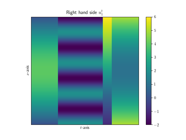
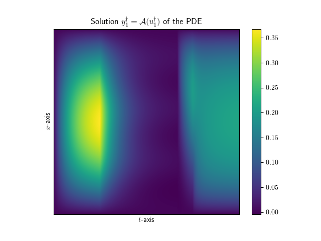
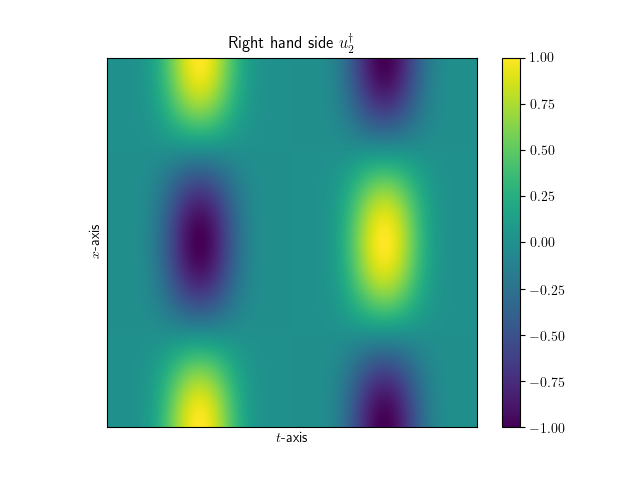
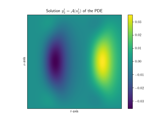
Figure 1: Solution of the PDE (1). First row, left: right hand side $u=u_{1}^{\dagger}$ as defined in (24). First row, right: corresponding solution $y_{1}:=\mathcal{A}(u_{1}^{\dagger})$. Second row, left: right hand side $u=u_{2}^{\dagger}$ as defined in (25). Second row, right: corresponding solution $y_{2}:=\mathcal{A}(u_{2}^{\dagger})$.

For the numerical tests of the algorithm and the regularization method, we have generated noisy data $n^{\delta}_{i}$ by sampling from an i.i.d. Gaussian random variable with mean $0$ and standard deviation $\sigma=\delta\lVert y_{i}\rVert_{L^{2}}$ and then defined $y_{i}^{\delta}=y_{i}+n_{i}^{\delta}$. Thus the noise level $\delta$ always refers to the relative noise level as compared to the true data $y_{i}=\mathcal{A}(u^{\dagger})$.

Figure 2 shows the reconstructions we obtain for a noise level $\delta=10^{-2}$ by solving (8). For the true solution $u_{1}^{\dagger}$, we have set the regularisation parameters to $\lambda=10^{-4}$ and $\mu=10^{-5}$; for the true solution $u_{2}^{\dagger}$ to $\lambda=2\cdot 10^{-6}$ and $\mu=10^{-5}$. The general shape of the true solution is well reconstructed, and the method is also able to reconstruct the jumps in the function $u_{1}^{\dagger}$, although the position of the jumps is not detected precisely. Also, the error is relatively large at the boundary of the domain, which can be explained by the fact that we solve the PDE (1) with Dirichlet boundary conditions. Thus the function $u^{\dagger}$ has only very little influence on $y^{\dagger}$ near the boundary, which makes it hard to reconstruct.

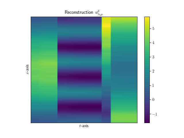
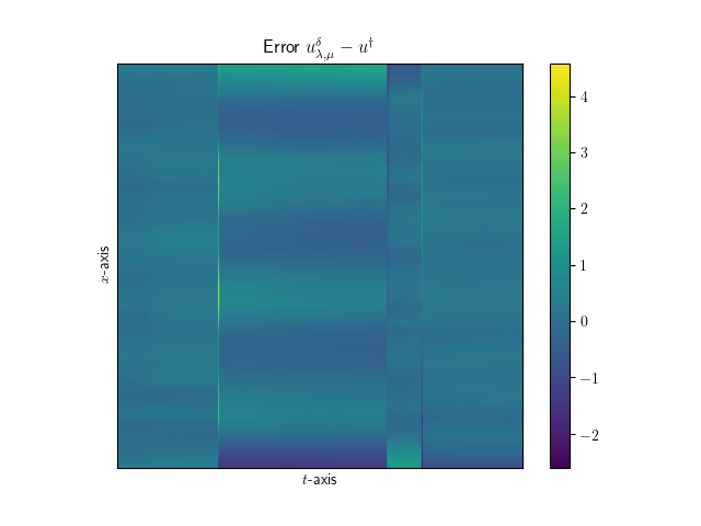
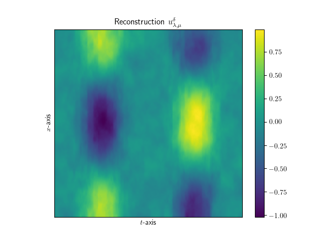
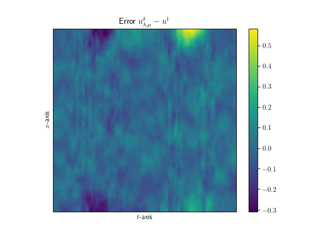
Figure 2: Regularised solution of (2) by the solution of (8). First row, left: regularised solution $u_{\lambda,\mu}^{\delta}$ with noisy data $y^{\delta}=u_{1}^{\dagger}+n^{\delta}$ with $u_{1}^{\dagger}$ as defined in (24), noise level $\delta=10^{-2}$, and regularisation parameters $\lambda=10^{-4}$ and $\mu=10^{-5}$. First row, right: resulting error $u_{\lambda,\mu}^{\delta}-u^{\dagger}$. Second row, left: regularised solution $u_{\lambda,\mu}^{\delta}$ with noisy data $y^{\delta}=u_{2}^{\dagger}+n^{\delta}$ with $u=u_{2}^{\dagger}$ as defined in (25), noise level $\delta=10^{-2}$, and regularisation parameters $\lambda=2\cdot 10^{-6}$ and $\mu=10^{-5}$. Second row, right: resulting error $u_{\lambda,\mu}^{\delta}-u^{\dagger}$.

Convergence of the algorithm

In order to demonstrate the convergence properties of Algorithm 2, we have applied the algorithm to a noisy version $y_{1}^{\delta}=y_{1}+n^{\delta}$ of $y_{1}$ with a noise level $\delta=0.01$. For the regularization parameters we chosen the values $\lambda=10^{-5}$ and $\mu=2\cdot 10^{-6}$. The number of iterations for the inner loop in Algorithm 2 was set to $k_{\text{max}}=5$.

Figure 3 (left) shows how the size of the updates $\lVert u^{\textrm{old}}-u\rVert$ changes over the iterations. We see how these step lengths roughly decrease linearly with the number of steps. In Figure 3 (right), we show the convergence behavior of the iterates towards the actual (numerical) solution of the variational inequality. For this, we have computed a numerical approximation to the actual solution $\hat{u}$ by running the algorithm for 10000 iterations. We see that the error decreases roughly linearly with the iterations. In addition, we see in 3 (middle) how the different term $\lVert\mathcal{A}(u)-y^{\delta}\rVert$, $\lambda\mathcal{R}(u)$, $\mu\mathcal{S}(u)$ change with the iterations.

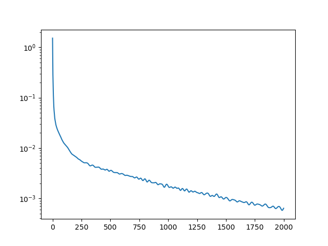
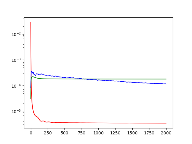
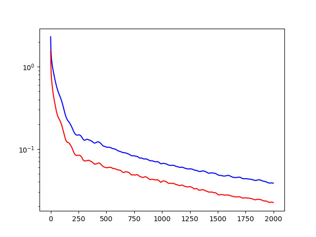
Figure 3: Demonstration of the convergence behavior of Algorithm 2. Left: Size of the updates $\lVert u^{(\text{old})}-u\rVert_{2}$. Middle: Values of the residual $\lVert\mathcal{A}(u)-y^{\delta}\rVert_{2}$ (red), the total variation regularization term $\lambda\mathcal{R}(u)$ (blue), and the $H^{1}$ regularization term $\mu\mathcal{S}(u)$ (green). Right: Errors $\lVert u-\hat{u}\rVert_{2}$ (blue) and $\lVert u-\hat{u}\rVert_{1}$ (red), where $\hat{u}$

Semi-convergence of the regularization method

Finally, we study the behavior of the regularized solutions as noise levels and regularization parameters simultaneously tend to $0$. According to Theorem 1, the regularized solutions converge in this case to the true solution, provided that the regularization parameters tend to $0$ in such a way that the ratios $\lambda/\delta$ and $\mu/\delta$ remain bounded.

In order to verify this result numerically, we have selected initial regularization parameters $\lambda_{0}$, $\mu_{0}>0$, and an initial noise level $\delta_{0}$. We have then applied our method with parameters $\lambda_{i}=2^{-i}\lambda_{0}$, $\mu_{i}=2^{-i}\mu_{0}$, and noise level $\delta_{i}=2^{-i}\delta_{0}$ to the two true solutions $u_{1}^{\dagger}$ and $u_{2}^{\dagger}$ defined in (24) and (25).

Figure 4 shows convergence plots for these experiments. We see there that the error $\lVert u-u_{i}^{\dagger}\rVert_{L^{2}}$ for both of the true solutions $u_{1}^{\dagger}$ and $u_{2}^{\dagger}$ roughly behaves like $O(\delta^{1/2})$ whereas the residual $\lVert\mathcal{A}(u)-u_{i}^{\dagger}\rVert_{L^{2}}$ behaves like $O(\delta)$. This is in agreement with the theory for standard Lavrentiev regularization for linear operators, where it is known that $O(\delta^{1/2})$ is the best possible rate for the error in non-trivial situations, see [29]. We note here, though, that as of now there exist no theoretical results concerning convergence rates with respect to the norm for our method. In [10], convergence rates with respect to the Bregman distance defined by $\mathcal{R}+\mathcal{S}$ have been derived. Because this functional is not strictly convex, let alone $p$-convex, these rates cannot be translated to rates in the $L^{2}$-norm, though. Also, it is not clear whether the variational source condition required in [10] holds for the test functions used for our experiments.

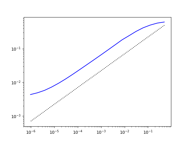
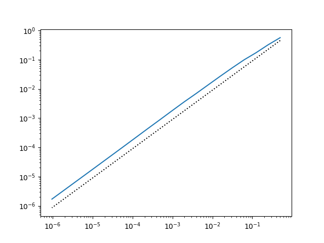
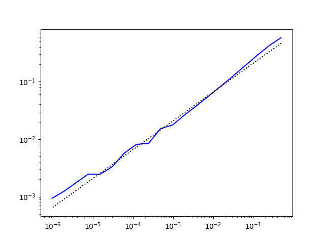
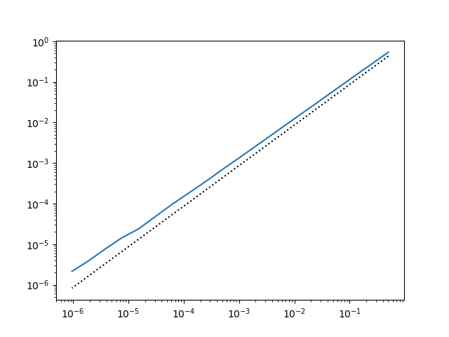
Figure 4: Convergence of the regularization method. Left: Plot of the relative error $\lVert u-u_{1}^{\dagger}\rVert_{2}/\lVert u_{1}^{\dagger}\rVert_{2}$ (blue). The black dotted line indicates a rate of order $\sqrt{\delta}$. Right: Plot of the relative residual $\lVert\mathcal{A}(u)-y_{1}\rVert_{2}/\lVert y_{1}\rVert_{2}$ (blue). The black dotted line indicates a rate of order $\delta$.

References

• \bibcommenthead
• Engl et al. [1996] Engl, H.W., Hanke, M., Neubauer, A.: Regularization of Inverse Problems. Mathematics and its Applications, vol. 375, p. 321. Kluwer Academic Publishers Group, Dordrecht (1996)
• Scherzer et al. [2009] Scherzer, O., Grasmair, M., Grossauer, H., Haltmeier, M., Lenzen, F.: Variational Methods in Imaging. Applied Mathematical Sciences, vol. 167, p. 320. Springer, New York (2009). https://doi.org/10.1007/978-0-387-69277-7
• Kaltenbacher et al. [2008] Kaltenbacher, B., Neubauer, A., Scherzer, O.: Iterative Regularization Methods for Nonlinear Ill-posed Problems. Radon Series on Computational and Applied Mathematics, vol. 6, p. 194. Walter de Gruyter GmbH & Co. KG, Berlin (2008). https://doi.org/10.1515/9783110208276
• Kaltenbacher [2016] Kaltenbacher, B.: Regularization based on all-at-once formulations for inverse problems. SIAM J. Numer. Anal. 54(4), 2594–2618 (2016) https://doi.org/10.1137/16M1060984
• Kunisch and Sachs [1992] Kunisch, K., Sachs, E.W.: Reduced SQP methods for parameter identification problems. SIAM J. Numer. Anal. 29(6), 1793–1820 (1992) https://doi.org/10.1137/0729100
• Hanke et al. [1995] Hanke, M., Neubauer, A., Scherzer, O.: A convergence analysis of the Landweber iteration for nonlinear ill-posed problems. Numer. Math. 72(1), 21–37 (1995) https://doi.org/10.1007/s002110050158
• Tautenhahn [2002] Tautenhahn, U.: On the method of Lavrentiev regularization for nonlinear ill-posed problems. Inverse Problems 18(1), 191–207 (2002) https://doi.org/10.1088/0266-5611/18/1/313
• Alber and Ryazantseva [2006] Alber, Y., Ryazantseva, I.: Nonlinear Ill-posed Problems of Monotone Type, p. 410. Springer, Dordrecht (2006)
• Hofmann et al. [2016] Hofmann, B., Kaltenbacher, B., Resmerita, E.: Lavrentiev’s regularization method in Hilbert spaces revisited. Inverse Probl. Imaging 10(3), 741–764 (2016) https://doi.org/10.3934/ipi.2016019
• Grasmair and Hildrum [2024] Grasmair, M., Hildrum, F.: Subgradient-based Lavrentiev regularisation of monotone ill-posed problems. Work in progress; an earlier version of this paper is available on arXiv at https://arxiv.org/abs/2005.08917 (2024)
• Bauschke and Combettes [2011] Bauschke, H.H., Combettes, P.L.: Convex Analysis and Monotone Operator Theory in Hilbert Spaces. CMS Books in Mathematics, p. 468. Springer, New York (2011). https://doi.org/10.1007/978-1-4419-9467-7
• Gautam et al. [2021] Gautam, P., Sahu, D.R., Dixit, A., Som, T.: Forward-backward-half forward dynamical systems for monotone inclusion problems with application to v-GNE. J. Optim. Theory Appl. 190(2), 491–523 (2021) https://doi.org/10.1007/s10957-021-01891-2
• Boţ et al. [2015] Boţ, R.I., Csetnek, E.R., Heinrich, A., Hendrich, C.: On the convergence rate improvement of a primal-dual splitting algorithm for solving monotone inclusion problems. Math. Program. 150(2), 251–279 (2015) https://doi.org/10.1007/s10107-014-0766-0
• Vũ [2013] Vũ, B.C.: A splitting algorithm for dual monotone inclusions involving cocoercive operators. Adv. Comput. Math. 38(3), 667–681 (2013) https://doi.org/10.1007/s10444-011-9254-8
• Lorenz and Pock [2015] Lorenz, D.A., Pock, T.: An inertial forward-backward algorithm for monotone inclusions. J. Math. Imaging Vision 51(2), 311–325 (2015) https://doi.org/%****␣ParIdPDE_MonIncl.tex␣Line␣1725␣****10.1007/s10851-014-0523-2
• Boţ and Csetnek [2016] Boţ, R.I., Csetnek, E.R.: An inertial forward-backward-forward primal-dual splitting algorithm for solving monotone inclusion problems. Numer. Algorithms 71(3), 519–540 (2016) https://doi.org/10.1007/s11075-015-0007-5
• Chambolle and Pock [2016] Chambolle, A., Pock, T.: On the ergodic convergence rates of a first-order primal-dual algorithm. Math. Program. 159(1-2), 253–287 (2016) https://doi.org/10.1007/s10107-015-0957-3
• Poljak [1964] Poljak, B.T.: Some methods of speeding up the convergence of iterative methods. Ž. Vyčisl. Mat i Mat. Fiz. 4, 791–803 (1964)
• Nesterov [1983] Nesterov, Y.E.: A method for solving the convex programming problem with convergence rate $O(1/k^{2})$. Dokl. Akad. Nauk SSSR 269(3), 543–547 (1983)
• Beck and Teboulle [2009] Beck, A., Teboulle, M.: A fast iterative shrinkage-thresholding algorithm for linear inverse problems. SIAM J. Imaging Sci. 2(1), 183–202 (2009) https://doi.org/10.1137/080716542
• Heida et al. [2019] Heida, M., Patterson, R.I.A., Renger, D.R.M.: Topologies and measures on the space of functions of bounded variation taking values in a Banach or metric space. J. Evol. Equ. 19(1), 111–152 (2019) https://doi.org/10.1007/s00028-018-0471-1
• Lions and Mercier [1979] Lions, P.-L., Mercier, B.: Splitting algorithms for the sum of two nonlinear operators. SIAM J. Numer. Anal. 16(6), 964–979 (1979) https://doi.org/%****␣ParIdPDE_MonIncl.tex␣Line␣1825␣****10.1137/0716071
• Abbas and Attouch [2015] Abbas, B., Attouch, H.: Dynamical systems and forward-backward algorithms associated with the sum of a convex subdifferential and a monotone cocoercive operator. Optimization 64(10), 2223–2252 (2015) https://doi.org/10.1080/02331934.2014.971412
• Chen and Loris [2019] Chen, J., Loris, I.: On starting and stopping criteria for nested primal-dual iterations. Numer. Algorithms 82(2), 605–621 (2019) https://doi.org/10.1007/s11075-018-0616-x
• Bonettini et al. [2023] Bonettini, S., Prato, M., Rebegoldi, S.: A nested primal-dual FISTA-like scheme for composite convex optimization problems. Comput. Optim. Appl. 84(1), 85–123 (2023) https://doi.org/10.1007/s10589-022-00410-x
• Attouch and Peypouquet [2016] Attouch, H., Peypouquet, J.: The rate of convergence of Nesterov’s accelerated forward-backward method is actually faster than $1/k^{2}$. SIAM J. Optim. 26(3), 1824–1834 (2016) https://doi.org/10.1137/15M1046095
• Moreau [1965] Moreau, J.-J.: Proximité et dualité dans un espace Hilbertien. Bull. Soc. Math. France 93, 273–299 (1965)
• Barbu [1976] Barbu, V.: Nonlinear Semigroups and Differential Equations in Banach Spaces, p. 352. Editura Academiei Republicii Socialiste România, Bucharest, Noordhoff International Publishing, Leiden (1976). Translated from the Romanian
• Plato [2017] Plato, R.: Converse results, saturation and quasi-optimality for Lavrentiev regularization of accretive problems. SIAM J. Numer. Anal. 55(3), 1315–1329 (2017) https://doi.org/%****␣ParIdPDE_MonIncl.tex␣Line␣1925␣****10.1137/16M1089125