mO#3m#1[#2]#3*

An Introduction to T-Systems

Samuel Karlin (June 8, 1924 – December 18, 2007)
He solved almost unnoticed an
important algebraic question.

These are the lecture notes based on dD (23) for the (upcoming) lecture T-systems with a special emphasis on sparse moment problems and sparse Positivstellensätze in the summer semester 2024 at the University of Konstanz.

The main purpose of this lecture is to prove the sparse Positiv- and Nichtnegativstellensätze of Samuel Karlin (1963) and to apply them to the algebraic setting. That means given finitely many monomials, e.g.

$$1,x^{2},x^{3},x^{6},x^{7},x^{9},$$

how do all linear combinations of these look like which are strictly positive or non-negative on some interval $[a,b]$ or $[0,\infty)$, e.g. describe and even write down all

$$f(x)=a_{0}+a_{1}x^{2}+a_{2}x^{3}+a_{3}x^{6}+a_{4}x^{7}+a_{5}x^{9}$$

with $f(x)>0$ or $f(x)\geq 0$ on $[a,b]$ or $[0,\infty)$, respectively.

To do this we introduce the theoretical framework in which this question can be answered: T-systems. We study these T-systems to arrive at Karlin’s Positiv- and Nichtnegativstellensatz but we also do not hide the limitations of the T-systems approach.

The main limitation is the Curtis–Mairhuber–Sieklucki Theorem which essentially states that every T-system is only one-dimensional and hence we can only apply these results to the univariate polynomial case. This can also be understood as a lesson or even a warning that this approach has been investigated and found to fail, i.e., learning about these results and limitations shall save students and researchers from following old footpaths which lead to a dead end.

We took great care finding the correct historical references where the results appeared first but are perfectly aware that like people before we not always succeed.

Konstanz,  
February 2024 Philipp J. di Dio

Acknowledgements

The author was supported by the Deutsche Forschungsgemeinschaft DFG with the grant DI-2780/2-1 and his research fellowship at the Zukunfskolleg of the University of Konstanz, funded as part of the Excellence Strategy of the German Federal and State Government.

The author thanks Konrad Schmüdgen for reading large parts of the manuscript and providing valuable remarks.

Contents

chapter*.1chapter*.2chapter*.3chapter.0section.0.1section.0.2section.0.3section.0.4section.0.5section.0.6section.0.7section.0.8section.0.9part.1chapter.1section.1.1section.1.2section*.6chapter.2section.2.1section.2.2section.2.3section.2.4section.2.5section*.7chapter.3section.3.1section.3.2section.3.3section.3.4section.3.5section*.8part.2chapter.4section.4.1section.4.2section.4.3section.4.4section.4.5section*.9chapter.5section.5.1section.5.2section.5.3section.5.4section.5.5section*.10chapter.6section.6.1section.6.2section.6.3section*.11part.3chapter.7section.7.1section.7.2section.7.3section*.14chapter.8section.8.1section.8.2section.8.3section.8.4section*.15part.4chapter.9section.9.1section.9.2section.9.3section*.24chapter.10section.10.1section.10.2section.10.3section.10.4section*.25part.5chapter.11section.11.1section.11.2chapter.12section.12.1section.12.2part*.34appendix*.35section*.36section*.37section*.38section*.39section*.40section*.42section*.43section*.44section*.45section*.46appendix*.47appendix*.48appendix*.52

Pure mathematics is, in its way, the poetry of logical ideas.
           Albert Einstein Ein (35)

Chapter 0 Preliminaries

The purpose of this preliminary chapter is not to establish and prove results but to clarify notation and to give the reader a survey of what will be assumed as known.

For the representation theorems of linear functionals of Daniell (0.17) and Riesz (0.18) more care is invested since these are the essential representation theorems in the theory of moments in the following chapters, i.e., we include the proofs.

1 Sets, Relations, and Orders

We let $\mathds{N}:=\{1,2,3,\dots\}$ be the natural numbers, $\mathds{N}_{0}:=\{0,1,2,\dots,\}$ be the natural numbers including zero, and as usual $\mathds{Z}$, $\mathds{Q}$, $\mathds{R}$, and $\mathds{C}$. The unit circle is denoted by $\mathds{T}:=\{(x,y)\in\mathds{R}^{2}\,|\,x^{2}+y^{2}=1\}$.

For inclusions we use $\subseteq$ and $\subsetneq$. To avoid any confusion we avoid the use of $\subset$ since $\subset$ is used in the literature by different authors either as $\subseteq$ or $\subsetneq$.

For a set $\mathcal{X}$ we denote by $\mathcal{P}(\mathcal{X})$ the set of all subsets of $\mathcal{X}$.

A partial order on a set $\mathcal{X}$ is a relation $R\subseteq\mathcal{X}\times\mathcal{X}$, usually denoted by $\leq$, such that

1. $x=y\quad\Leftrightarrow\quad x\leq y$ and $y\leq x$,

2. $x\leq y$ and $y\leq z\quad\Rightarrow\quad x\leq z$.

A relation $\leq$ is a total order if for all $x,y\in\mathcal{X}$ we have either $x\leq y$ or $y\leq x$. A vector space $E$ with a partial order $\leq$ such that

1. $x\leq y$ and $z\in\mathcal{X}\quad\Rightarrow\quad x+z\leq y+z$,

2. $x\leq y$ and $a\in[0,\infty)\quad\Rightarrow\quad ax\leq ay$

is called an ordered vector space. If $E$ is an ordered vector space then $E_{+}:=\{x\in E\,|\,0\leq x\}$ denotes the positive cone and $E_{-}:=\{x\in E\,|\,x\leq 0\}$ denoted the negative cone. Let $C\subseteq E$ be a cone in a vector space $E$. Then $E$ with $x\leq y$ if and only if $y-x\in C$ is a (partially) ordered vector space.

For a vector space $E$ a (linear) function $f:E\to\mathds{R}$ is called (linear) functional. For a vector space $E$ the (algebraic) dual $E^{*}$ is the set of all linear functionals $f:E\to\mathds{R}$. A functional $f:E\to\mathds{R}$ is called sublinear if $f(\rho x)\leq\rho f(x)$ and $f(x+y)\leq f(x)+f(y)$ hold for all $\rho\geq 0$ and $x,y\in E$. It is called superlinear if $-f$ is sublinear.

Hahn–Banach Theorem 0.1.

Let $\mathcal{X}$ be a real vector space, let $p:\mathcal{X}\to\mathds{R}$ be a sublinear function, $\mathcal{V}\subseteq\mathcal{X}$ be a subspace, and $f:\mathcal{V}\to\mathds{R}$ be a linear functional such that $f(x)\leq p(x)$ for all $x\in\mathcal{V}$. Then there exists a linear functional $F:\mathcal{X}\to\mathds{R}$ such that

1. $f(x)=F(x)$ for all $x\in\mathcal{V}$, and

2. $F(x)\leq p(x)$ for all $x\in\mathcal{X}$.

The 0.1 was proved by H. Hahn Hah (27) and S. Banach Ban29a ; Ban29b . A previous version is due to E. Helly Hel (12). For more see e.g. Pie (07) or standard functional analysis textbooks like Yos (68); Wer (07).

2 Topology

A topology $\mathcal{T}$ on a set $\mathcal{X}$ is a set $\mathcal{T}\subseteq\mathcal{P}(\mathcal{X})$ of subsets of $\mathcal{X}$ which is closed under finite intersections and arbitrary unions, i.e., especially $\emptyset,\mathcal{X}\in\mathcal{T}$. $(\mathcal{X},\mathcal{T})$ is called a topological space and sets $A\in\mathcal{T}$ are called open. A set $A\subseteq\mathcal{X}$ is called closed if $\mathcal{X}\setminus A$ is open. The interior $\mathrm{int}\,A$ of a set $A\subseteq\mathcal{X}$ is the union of all open sets $O\subseteq A$. A subset $U$ of a topological space $(\mathcal{X},\mathcal{T})$ is called a neighborhood of $x$ if $x\in\mathrm{int}\,U$.

A function $f:\mathcal{X}\to\mathcal{Y}$ between two topological spaces $\mathcal{X}$ and $\mathcal{Y}$ is called continuous at $x\in\mathcal{X}$ if for each neighborhood $V$ of $y=f(x)$ the set $f^{-1}(y)$ is a neighborhood of $x$. The function $f$ is called continuous if it is continuous at every $x\in\mathcal{X}$. The set of continuous functions $f:\mathcal{X}\to\mathcal{Y}$ is denoted by $\mathcal{C}(\mathcal{X},\mathcal{Y})$. A set $K\subseteq\mathcal{X}$ is called compact if every open cover $K\subseteq\bigcup_{i\in I}U_{i}$, $U_{i}\in\mathcal{T}$, has a finite subcover $K\subseteq\bigcup_{k=1}^{n}U_{i_{k}}$. For a function $f:\mathcal{X}\to\mathds{R}$ we have the support $\mathrm{supp}\,f:=\{x\in\mathcal{X}\,|\,f(x)\neq 0\}$. The set of all continuous functions with compact support are denoted by $\mathcal{C}_{c}(\mathcal{X},\mathds{R})$.

A topological space $\mathcal{X}$ is called Hausdorff space if each pair of distinct points $x,y\in\mathcal{X}$ have disjoint neighborhoods. A Hausdorff space $\mathcal{X}$ is called locally compact if every point $x\in\mathcal{X}$ has a compact neighborhood. On Hausdorff spaces we have the following important topological result.

Urysohn’s Lemma 0.2 (see Ury (25)).

Let $\mathcal{X}$ be a Hausdorff space. The following are equivalent:

1. For every pair of disjoint closed sets $A,B\subseteq\mathcal{X}$ there exist a neighborhood $U$ of $A$ and a neighborhood $V$ of $B$ such that $U\cap V=\emptyset$.

2. For each pair $A,B\subseteq\mathcal{X}$ of disjoint closed sets there exists a continuous function $f:\mathcal{X}\to[0,1]$ such that $f(x)=1$ for all $x\in A$ and $f(y)=0$ for all $y\in B$.

3 Stone–Weierstrass Theorem

Stone–Weierstrass Theorem 0.3 (Wei (85) and (Sto, 37, pp. 467–468) or e.g. (Yos, 68, p. 9)).

Let $\mathcal{X}$ be a compact set and let $B\subseteq\mathcal{C}(X,\mathds{R})$ be such that

1. $fg,\alpha f+\beta g\in B$ for all $f,g\in B$ and $\alpha,\beta\in\mathds{R}$,

2. there exists a $f\in B$ with $f>0$ on $\mathcal{X}$, and

3. for all $x,y\in\mathcal{X}$ with $x\neq y$ there is a $f\in B$ such that $f(x)\neq f(y)$

then for any $f\in\mathcal{C}(\mathcal{X},\mathds{R})$ there exists $\{f_{n}\}_{n\in\mathds{N}_{0}}\subseteq B$ such that

$$\|f-f_{n}\|_{\infty}\xrightarrow{n\to\infty}0.$$

Especially $\mathds{R}[x_{1},\dots,x_{n}]$ on any compact $K\subseteq\mathds{R}^{n}$, $n\in\mathds{N}$, is dense in $\mathcal{C}(K,\mathds{R})$ in the $\sup$-norm.

For more on the history of the 0.3 see e.g. (Pie, 07, §4.5.6–§4.5.8).

4 Convex Geometry

A set $\mathcal{X}$ is convex if $\lambda x+(1-\lambda)y\in\mathcal{X}$ for all $x,y\in\mathcal{X}$ and $\lambda\in[0,1]$. A set $\mathcal{X}$ is a cone if $\lambda x\in\mathcal{X}$ for all $x\in\mathcal{X}$ and $\lambda\in[0,\infty)$. For a set $A\subseteq\mathds{R}^{n}$ we denote by $\mathrm{conv}\,A$ the convex hull of $A$.

Carathéodory’s Theorem 0.4 (see Car (11)).

Let $n\in\mathds{N}$ and let $S\subseteq\mathds{R}^{n}$ be a set. If $x\in\mathrm{conv}\,A$ then there is a $k\leq n+1$, points $x_{1},\dots,x_{k}\in A$, and $\lambda_{1},\dots,\lambda_{k}>0$ with

$$x=\lambda_{1}x_{1}+\dots+\lambda_{k}x_{k}\qquad\text{and}\qquad\lambda_{1}+\dots+\lambda_{k}=1.$$

For more on convex geometry we recommend Roc (72) and Sch (14).

5 Linear Algebra

A matrix $M=(a_{i,j})_{i,j=1}^{n}$ with $a_{i,j}=a_{k,l}$ if $i+j=k+l$ is called Hankel matrix. For a sequence $s=(s_{\alpha})_{\alpha\in\mathds{N}_{0}:|\alpha|\leq 2n}$ with $n\in\mathds{N}_{0}$ we denote by

$$\mathcal{H}(s):=(s_{\alpha+\beta})_{\alpha,\beta\in\mathds{N}_{0}:|\alpha|,|\beta|\leq n}$$ (1)

the Hankel matrix of $s$.

6 Measures

For a set $\mathcal{X}$ an algebra $\mathfrak{A}$ is a set $\mathfrak{A}\subseteq\mathcal{P}(\mathcal{X})$ such that $\emptyset,\mathcal{X}\in\mathfrak{A}$ and for all $A,B\in\mathfrak{A}$ we have $A\cap B,A\cup B,A\setminus B\in\mathfrak{A}$. If additionally $\bigcup_{n=1}^{\infty}A_{n}\in\mathfrak{A}$ for all $A_{n}\in\mathfrak{A}$ then $\mathfrak{A}$ called a $\sigma$-algebra and $(\mathcal{X},\mathfrak{A})$ is called a measurable space. By $\mathfrak{B}(\mathds{R}^{n})$ we denote the Borel $\sigma$-algebra. For $A\subseteq\mathcal{P}(\mathcal{X})$ we denote by $\sigma(A)$ the smallest $\sigma$-algebra containing $A$. A function $f:(\mathcal{X},\mathfrak{A})\to(\mathcal{Y},\mathfrak{B})$ between two measurable spaces is called measurable if $f^{-1}(B)\in\mathfrak{A}$ for all $B\in\mathfrak{B}$.

A measure $\mu$ is a function $\mu:\mathfrak{A}\to[0,\infty]$ on an algebra $\mathfrak{A}$ such that $\mu$ is countably additive, i.e.,

$$\mu\left(\bigcup_{n=1}^{\infty}A_{n}\right)=\sum_{n=1}^{\infty}\mu(A_{n})$$

for all pairwise disjoint sets $A_{n}\in\mathfrak{A}$. A measure $\mu$ on $\mathfrak{B}(\mathds{R}^{n})$ is called Borel measure. A Borel measure $\mu$ is called a Radon measure if for every $A\in\mathfrak{B}(\mathds{R}^{n})$ and $\varepsilon>0$ there exists a compact set $K_{\varepsilon}\subseteq A$ such that $\mu(A\setminus K_{\varepsilon})<\varepsilon$. We denote by $\mathcal{M}(\mathcal{X})_{+}$ the set of all Borel measures on $(\mathcal{X},\mathfrak{A})$. By $(\mathcal{X},\mathfrak{A},\mu)$ we denote a measure space. A measurable function $f:(\mathcal{X},\mathfrak{A})\to\mathds{R}$ is called $\mu$-integrable if

$$\int_{\mathcal{X}}|f(x)|~{}\mathrm{d}\mu(x)<\infty.$$

For any $p\geq 1$ we denote by $\mathcal{L}^{p}(\mathcal{X},\mu)$ all $\mu$-integrable functions on $\mathcal{X}$. For $p=\infty$, i.e., $\mathcal{L}^{\infty}(\mathcal{X},\mu)$, the essential supremum is bounded.

Since we are proving the (signed) Daniell’s Theorem and the (signed) Riesz’ Representation Theorem we will give a more detailed background on measures. For more on measure theory we recommend Bog (07) and Fed (69).

Definition 0.5.

Let $\mathcal{X}$ be a set. A function $\mu:\mathcal{P}(\mathcal{X})\to[0,\infty]$ with

1. $\mu(\emptyset)=0$,

2. $\mu(A)\leq\mu(B)$ for all $A\subseteq B\subseteq\mathcal{X}$, and

3. $\mu\left(\bigcup_{i=1}^{\infty}A_{i}\right)\leq\sum_{i=1}^{\infty}\mu(A_{i})$ for all $A_{i}\in\mathcal{X}$

is called a (Carathéodory) outer measure.

Definition 0.6.

For an outer measure $\mu$ on $\mathcal{X}$ a set $A\subseteq\mathcal{X}$ is called (Carathéodory) $\mu$-measurable if for every $E\subseteq\mathcal{X}$ we have $\mu(E)=\mu(E\cap A)+\mu(E\setminus A)$.

Remark 0.7.

Since by 0.5 (iii) we always have

$$\mu(E)=\mu((E\cap A)\cup(E\setminus A))\leq\mu(E\cap A)+\mu(E\setminus A)$$

it is sufficient for $\mu$-measurability to test

$$\mu(E)\geq\mu(E\cap A)+\mu(E\setminus A).$$ (2)

An outer measure is in fact a measure on all its measurable sets.

Theorem 0.8.

Let $\mu$ be an outer measure on a set $\mathcal{X}$ and $\mathcal{A}_{\mu}\subseteq\mathcal{P}(\mathcal{X})$ be the set of all $\mu$-measurable sets. Then $\mathcal{A}_{\mu}$ is a $\sigma$-algebra of $\mathcal{X}$ and $\mu$ is a measure on $(\mathcal{X},\mathcal{A}_{\mu})$.

Proof.

See e.g. (Bog, 07, Thm. 1.11.4 (iii)). ∎

Outer measures give another characterization of measurable functions.

Lemma 0.9.

Let $\mu$ be an outer measure on $\mathcal{X}$ and $f:\mathcal{X}\to[-\infty,\infty]$ be a function. Then $f$ is $\mu$-measurable if and only if

$$\mu(A)\geq\mu(\{x\in A\,|\,f(x)\leq a\})+\mu(\{x\in A\,|\,f(x)\geq b\})$$

for all $A\subseteq\mathcal{X}$ and $-\infty<a<b<\infty$.

Proof.

See e.g. (Fed, 69, §2.3.2(7), pp. 74–75). ∎

Definition 0.10.

An outer measure $\mu$ is called regular if for each set $A\subseteq\mathcal{X}$ there exists a $\mu$-measurable set $B\subseteq\mathcal{X}$ with $A\subseteq B$ and $\mu(A)=\mu(B)$.

Definition 0.11.

Let $f,g:(\mathcal{X},\mathcal{A})\to\mathds{R}$ be two functions. Then we define $\inf(f,g)$ by

$$\inf(f,g)(x):=\inf(f(x),g(x))$$

for all $x\in\mathcal{X}$ and similarly $\sup(f,g)$. Additionally, $f\leq g$ iff $f(x)\leq g(x)$ for all $x\in\mathcal{X}$. We have $f_{+}:=\sup(f,0)$, $f_{-}:=f-f_{+}$, and $|f|=f_{+}-f_{-}$.

Definition 0.12.

Let $\mathcal{X}$ be a set. We call a set $\mathcal{F}$ of functions $f:\mathcal{X}\to\mathds{R}$ a lattice (of functions) if the following holds:

1. $c\cdot f\in\mathcal{F}$ for all $c\geq 0$ and $f\in\mathcal{F}$,

2. $f+g\in\mathcal{F}$ for all $f,g\in\mathcal{F}$,

3. $\inf(f,g)\in\mathcal{F}$ for all $f,g\in\mathcal{F}$,

4. $\inf(f,c)\in\mathcal{F}$ for all $c\geq 0$ and $f\in\mathcal{F}$, and

5. $g-f\in\mathcal{F}$ for all $f,g\in\mathcal{F}$ with $f\leq g$.

Some authors require that a lattice of functions is a vector space (lattice space). But for proving 0.15 it is only necessary that a lattice is a convex cone as in 0.12.

Example 0.13.

Let $\mathcal{X}$ be a locally compact Hausdorff space. Then $\mathcal{C}_{c}(\mathcal{X},\mathds{R})$ is a lattice of functions and even a lattice space. $\circ$

Given a lattice $\mathcal{F}$ we get another lattice $\mathcal{F}_{+}$ by taking only the non-negative functions.

Lemma 0.14 (see e.g. (Fed, 69, §2.5.1, p. 91)).

Let $\mathcal{F}$ be a non-empty lattice on a set $\mathcal{X}$ and define

$$\mathcal{F}_{+}:=\{f\in\mathcal{F}\,|\,f\geq 0\}.$$

Then

1. $f_{+},f_{-},|f|\in\mathcal{F}_{+}$ for all $f\in\mathcal{F}$ and

2. $\mathcal{F}_{+}$ is a non-empty lattice on $\mathcal{X}$.

Proof.

(i): Since $\inf(f,0)\in\mathcal{F}$ and $\inf(f,0)\leq f$ we have $f_{+}=\sup(f,0)=f-\inf(f,0)\in\mathcal{F}_{+}$ for all $f\in\mathcal{F}$. Since $f\leq f_{+}=\sup(f,0)\in\mathcal{F}$ we have $f_{-}=f_{+}-f\in\mathcal{F}_{+}$ for all $f\in\mathcal{F}$. It follows that $|f|=f_{+}+f_{-}\in\mathcal{F}_{+}$ for all $f\in\mathcal{F}$.

(ii): Since $\mathcal{F}$ is non-empty there is a $f\in\mathcal{F}$ and by (ii) we have $|f|\in\mathcal{F}$ and hence $|f|\in\mathcal{F}_{+}$. $\mathcal{F}_{+}$ is a lattice by directly checking the 0.12. ∎

7 Daniell’s Representation Theorem

The question when a linear functional acting on (not necessarily measurable) functions is represented by a measure was already fully answered by P. J. Daniell in 1918 Dan (18), see also Dan (20).

Nowadays only the 0.20 is given in standard texts for the moment problem. We therefore take the time to present also Daniell’s approach which is more general and has some interesting features the standard 0.20 does not have.

Note, that $h_{n}\nearrow g$ denotes a sequence $(h_{n})_{n\in\mathds{N}}$ with $h_{1}\leq h_{2}\leq...\leq g$, i.e., point-wise non-decreasing, with $\lim_{n\to\infty}h_{n}(x)=g(x)$ for all $x\in\mathcal{X}$. Equivalently, $h_{n}\searrow 0$ denotes a point-wise non-increasing sequence with $\lim_{n\to\infty}h_{n}(x)=0$ for all $x\in\mathcal{X}$.

Daniell’s Representation Theorem 0.15 (Dan (18), see also Dan (20) or (Fed, 69, Thm. 2.5.2)).

Let $\mathcal{F}$ be a lattice of functions on a set $\mathcal{X}$ and let $L:\mathcal{F}\to\mathds{R}$ be such that

1. $L(f+g)=L(f)+L(g)$ for all $f,g\in\mathcal{F}$,

2. $L(c\cdot f)=c\cdot L(f)$ for all $c\geq 0$ and $f\in\mathcal{F}$,

3. $L(f)\leq L(g)$ for all $f,g\in\mathcal{F}$ with $f\leq g$,

4. $L(f_{n})\nearrow L(g)$ as $n\to\infty$ for all $g\in\mathcal{F}$ and $f_{n}\in\mathcal{F}$ with $f_{n}\nearrow g$.

Then there exists a measure $\mu$ on $(\mathcal{X},\mathcal{A})$ with

$$\mathcal{A}:=\sigma(\{f^{-1}((-\infty,a])\,|\,a\in\mathds{R},\ f\in\mathcal{F}\})$$ (3)

such that

$$L(f)=\int_{\mathcal{X}}f(x)~{}\mathrm{d}\mu(x)$$

for all $f\in\mathcal{F}$.

We follow the proof in (Fed, 69, Thm. 2.5.2, pp. 92–93).

Proof.

By assumption (iii) we have $L(f)\geq L(0\cdot f)=0$ for all $f\in\mathcal{F}_{+}$.

For any $A\subseteq\mathcal{X}$ we say a sequence $(f_{n})_{n\in\mathds{N}}$ suits $A$ if and only if $f_{n}\in\mathcal{F}_{+}$ and $f_{n}\leq f_{n+1}$ for all $n\in\mathds{N}$ and

$$\lim_{n\to\infty}f_{n}(x)\geq 1\qquad\text{for all}\ x\in A.$$

Note, that we can even assume equality by replacing the $f_{n}$’s by $\tilde{f}_{n}:=\inf(f_{n},1)\in\mathcal{F}_{+}$. Then we define

$$\mu(A):=\inf\left\{\lim_{n\to\infty}L(f_{n})\;\middle|\;(f_{n})_{n\in\mathds{N}}\ \text{suits}\ A\right\}$$ (4)

which is $\infty$ if there is no sequence $(f_{n})_{n\in\mathds{N}}$ that suits $A$.

We prove that $\mu$ is an outer measure, see 0.5. By assumption (iii) $L(f_{n})$ is a non-negative increasing sequence and therefore $\lim_{n\to\infty}L(f_{n})$ exists and is in $[0,\infty]$. Hence, $\mu:\mathcal{P}(\mathcal{X})\to[0,\infty]$. For $A=\emptyset$ the zero sequence $f_{n}=0\in\mathcal{F}_{+}$ is suited and therefore $\mu(\emptyset)=0$. Let $A\subseteq B\subseteq\mathcal{X}$, then a suited sequence $(f_{n})_{n\in\mathds{N}}$ of $B$ is also a suited sequence for $A$ and therefore $\mu(A)\leq\mu(B)$. Let $A_{i}\subseteq\mathcal{X}$, $i\in\mathds{N}$, and set $A:=\bigcup_{i=1}^{\infty}A_{i}$. Any suited sequence for $A$ is a suited sequences for all $A_{i}$. Assume there is an $A_{i}$ which has no suited sequence, then $A$ has no suited sequence and $\mu(A)=\infty\leq\sum_{i=1}^{\infty}\mu(A_{i})=\infty$. So assume all $A_{i}$ have suited sequences, say $(f_{i,n})_{n\in\mathds{N}}$ suits $A_{i}$, $i\in\mathds{N}$. Then $f_{n}:=\sum_{i=1}^{n}f_{i,n}$ suits $A$ and

$$\mu(A)\leq\lim_{n\to\infty}L(f_{n})=\lim_{n\to\infty}\sum_{i=1}^{n}L(f_{i,n})\leq\sum_{i=1}^{\infty}\lim_{m\to\infty}L(f_{i,m}).$$

Taking the infimum on the right side for all $A_{i}$’s retains the inequality and gives

$$\mu\left(\bigcup_{i=1}^{\infty}A_{i}\right)=\mu(A)\leq\sum_{i=1}^{\infty}\mu(A_{i}).$$

Hence, all conditions in 0.5 are fulfilled and $\mu$ is an outer measure.

Since $\mu$ is an outer measure on $\mathcal{X}$ by 0.8 the set $\tilde{\mathcal{A}}$ of all $\mu$-measurable sets of $\mathcal{X}$ is a $\sigma$-algebra and $\mu$ is a measure on $(\mathcal{X},\tilde{\mathcal{A}})$.

It remains to show that all $f\in\mathcal{F}$ are $\mu$-measurable, $\mu$ is a measure on $(\mathcal{X},\mathcal{A})$ with $\mathcal{A}=\sigma(\{f^{-1}((-\infty,a])\,|\,a\in\mathds{R},\ f\in\mathcal{F}\})$, and $L(f)=\int_{\mathcal{X}}f(x)~{}\mathrm{d}\mu(x)$ for all $f\in\mathcal{F}$.

Since $f=f_{+}-f_{-}$ with $f_{+},f_{-}\in\mathcal{F}_{+}$ it is sufficient to show that every function in $\mathcal{F}_{+}$ is $\mu$-measurable. So let $f\in\mathcal{F}_{+}$. To show that $f$ is $\mu$-measurable it is sufficient to show that $A:=f^{-1}((-\infty,a])=\{x\in\mathcal{X}\,|\,f(x)\leq a\}\in\mathcal{A}$ for all $a\in\mathds{R}$, i.e., $A$ is $\mu$-measurable by 0.6 resp. 0.7 if (2) holds for all $E\subseteq\mathcal{X}$. From $E\setminus A=E\cap(\mathcal{X}\setminus A)=E\cap\{x\in\mathcal{X}\,|\,f(x)>a\}$ we have to verify

$$\mu(E)\geq\mu\big{(}\{x\in E\,|\,f(x)\leq a\}\big{)}+\mu\big{(}\{x\in E\,|\,f(x)>a\}\big{)}$$

and by 0.9 this is equivalent to

$$\mu(E)\geq\mu\big{(}\underbrace{\{x\in E\,|\,f(x)\leq a\}}_{=:E_{a}}\big{)}+\mu\big{(}\underbrace{\{x\in E\,|\,f(x)\geq b\}}_{=:E_{b}}\big{)}$$ (5)

for all $a<b$. For $a<0$ or $\mu(E)=\infty$ (5) is trivial, so assume $a\geq 0$ and $\mu(E)<\infty$.

Let $(g_{n})_{n\in\mathds{N}}$ be a sequence that suits $E$ and set

$$h:=(b-a)^{-1}\cdot[\inf(f,b)-\inf(f,a)]\in\mathcal{F}_{+}\qquad\text{and}\qquad k_{n}:=\inf(g_{n},h)\in\mathcal{F}_{+}.$$

Then we have $0\leq k_{n+1}-k_{n}\leq g_{n+1}-g_{n}$,

$$h(x) =1\qquad\text{for all}\ x\in\mathcal{X}\ \text{with}\ f(x)\geq b,$$

and

$$h(x) =0\qquad\text{for all}\ x\in\mathcal{X}\ \text{with}\ f(x)\leq a.$$

It follows that $(k_{n})_{n\in\mathds{N}}$ suits $E_{b}$ and $(g_{n}-k_{n})_{n\in\mathds{N}}$ suits $E_{a}$. Therefore,

$$\lim_{n\to\infty}L(g_{n})=\lim_{n\to\infty}[L(g_{n}-k_{n})+L(k_{n})]\geq\mu(E_{a})+\mu(E_{b})$$

and taking the infimum on the left side retains the inequality and proves (5). Hence, all $f\in\mathcal{F}_{+}$ and therefore all $f\in\mathcal{F}$ are $\mu$-measurable.

Let us show that $\mu$ remains a measure on $(\mathcal{X},\mathcal{A})$. Since all $f\in\mathcal{F}$ are $\mu$- and $\mathcal{A}$-measurable we have

$$f^{-1}((-\infty,a])\in\tilde{\mathcal{A}}$$

for all $a\in\mathds{R}$ and $f\in\mathcal{F}$. Therefore,

$$\mathcal{A}=\sigma(\{f^{-1}((-\infty,a])\,|\,a\in\mathds{R},\ f\in\mathcal{F}\})\subseteq\tilde{\mathcal{A}}$$

is a $\sigma$-algebra and we can restrict $\mu$ resp. $\tilde{\mathcal{A}}$ to $\mathcal{A}$. $\mu$ is a measure on $(\mathcal{X},\mathcal{A})$.

We show that $L(f)=\int_{\mathcal{X}}f(x)~{}\mathrm{d}\mu(x)$ holds for all $f\in\mathcal{F}_{+}$. Let $f\in\mathcal{F}_{+}$ and set

$$f_{t}:=\inf(f,t)$$

for $t\geq 0$. If $\varepsilon>0$ and $k\in\mathds{N}$ then

$$0\leq f_{k\varepsilon}(x)-f_{(k-1)\varepsilon}(x) \leq\varepsilon\quad\text{for all}\ x\in\mathcal{X},$$

$$f_{k\varepsilon}(x)-f_{(k-1)\varepsilon}(x) =\varepsilon\quad\text{for all}\ x\in\mathcal{X}\ \text{with}\ f(x)\geq k\varepsilon,$$

and

$$f_{k\varepsilon}(x)-f_{(k-1)\varepsilon}(x) =0\quad\text{for all}\ x\in\mathcal{X}\ \text{with}\ f(x)\leq(k-1)\varepsilon.$$

The constant sequence $(\varepsilon^{-1}\cdot(f_{k\varepsilon}-f_{(k-1)\varepsilon}))_{n\in\mathds{N}}$ suits $\{x\in\mathcal{X}\,|\,f(x)\geq k\varepsilon\}$ and consequently

$$L(f_{k\varepsilon}-f_{(k-1)\varepsilon}) \geq\varepsilon\cdot\mu(\{x\in\mathcal{X}\,|\,f(x)\geq k\varepsilon\})$$

$$\geq\int_{\mathcal{X}}f_{(k+1)\varepsilon}(x)-f_{k\varepsilon}(x)~{}\mathrm{d}\mu(x)$$

$$\geq\varepsilon\cdot\mu(\{x\in\mathcal{X}\,|\,f(x)\geq(k+1)\varepsilon\}) \geq L(f_{(k+2)\varepsilon}-f_{(k+1)\varepsilon}).$$

Summing with respect to $$k 1 n$$ from to we find

$$L(f_{n\varepsilon}) \geq\;\;\int_{\mathcal{X}}f_{(n+1)\varepsilon}(x)-f_{\varepsilon}(x)~{}\mathrm{d}\mu(x) \geq L(f_{(n+2)\varepsilon}-f_{2\varepsilon})$$

and since $$f_{n\varepsilon}\nearrow f n\to\infty n\to\infty$$ as we get from assumption (iv) for

$$L(f) \geq\qquad\int_{\mathcal{X}}f(x)-f_{\varepsilon}(x)~{}\mathrm{d}\mu(x) \geq L(f-f_{2\varepsilon})$$

which gives again from assumption (iv) for $$\varepsilon\searrow 0$$

$$L(f) \geq\qquad\quad\;\int_{\mathcal{X}}f(x)~{}\mathrm{d}\mu(x) \geq L(f).$$

Hence, $L(f)=\int_{\mathcal{X}}f(x)~{}\mathrm{d}\mu(x)$ for all $f\in\mathcal{F}_{+}$.

Finally, for all $f\in\mathcal{F}$ we have $f=f_{+}-f_{-}$ with $f_{+},f_{-}\in\mathcal{F}_{+}$ which implies

$$\int_{\mathcal{X}}f(x)~{}\mathrm{d}\mu(x)=\int_{\mathcal{X}}f_{+}(x)~{}\mathrm{d}\mu(x)-\int_{\mathcal{X}}f_{-}(x)~{}\mathrm{d}\mu(x)=L(f_{+})-L(f_{-})=L(f)$$

where the last equality follows from $f_{+}=f+f_{-}$ and assumption (i). ∎

The most impressive part is that the functional $L:\mathcal{F}\to\mathds{R}$ lives only on a lattice $\mathcal{F}$ of functions $f:\mathcal{X}\to\mathds{R}$ where $\mathcal{X}$ is a set without any structure. 0.15 provides a representing measure $\mu$ by (4) including the $\sigma$-algebra $\mathcal{A}$ of the measurable space $(\mathcal{X},\mathcal{A})$ by (3).

Remark 0.16.

In 0.15 the assumption (iv) is equivalent to

1. $L(h_{n})\searrow 0$ as $n\to\infty$ for all $h_{n}\in\mathcal{F}$ with $h_{n}\searrow 0$ as $n\to\infty$

since $f_{n}\nearrow g$ implies $f_{n}\leq g$ and $0\leq h_{n}=g-f_{n}\in\mathcal{F}$:

$$L(g)=L(g-f_{n}+f_{n})=L(g-f_{n})+\underbrace{L(f_{n})}_{\nearrow L(g)}=\underbrace{L(h_{n})}_{\searrow 0}\ +\ L(f_{n}).$$

The representing measure $\mu$ in 0.15 is not unique. But the representing measure $\mu$ constructed in (4) has further properties, see e.g. (Fed, 69, §2.5.3).

0.15 also has a signed version.

Signed Daniell’s Representation Theorem 0.17 (Dan (18), see also (Fed, 69, Thm. 2.5.5)).

Let $\mathcal{F}$ be a lattice of functions on some set $\mathcal{X}$ and let $L:\mathcal{F}\to\mathds{R}$ be such that for all $f,g,h_{1},h_{2},h_{3},{\dots}\in\mathcal{F}$ we have

1. $L(f+g)=L(f)+L(g)$,

2. $L(c\cdot f)=c\cdot L(f)$ for all $c\geq 0$,

3. $\sup L\big{(}\{k\in\mathcal{F}\,|\,0\leq k\leq f\}\big{)}<\infty$,

4. $h_{n}\nearrow g$ as $n\to\infty$ implies $L(h_{n})\to L(g)$ as $n\to\infty$.

Let $L_{+}$ and $L_{-}$ be the functionals on $\mathcal{F}_{+}$ defined by

$$L_{+}(f):=\sup L\big{(}\{k\in\mathcal{F}\,|\,0\leq k\leq f\}\big{)}$$

and

$$L_{-}(f):=-\inf L\big{(}\{k\in\mathcal{F}\,|\,0\leq k\leq f\}\big{)}$$

for all $f\in\mathcal{F}_{+}$. Then there exist $\mathcal{F}_{+}$ regular measures $\mu_{+}$ and $\mu_{-}$ on $\mathcal{X}$ such that

1. $L_{+}(f)=\int_{\mathcal{X}}f(x)~{}\mathrm{d}\mu_{+}(x)$ for all $f\in\mathcal{F}_{+}$,

2. $L_{-}(f)=\int_{\mathcal{X}}f(x)~{}\mathrm{d}\mu_{-}(x)$ for all $f\in\mathcal{F}_{+}$, and

3. $L(f)=L_{+}(f)-L_{-}(f)$ for all $f\in\mathcal{F}$.

The proof is taken from (Fed, 69, pp. 96–97) and uses 0.15.

Proof.

Let $f_{+}\in\mathcal{F}_{+}$. Then $f\geq g\in\mathcal{F}_{+}$ implies $f\geq f-g\in\mathcal{F}_{+}$ and

$$L(g)-L_{-}(f)\leq L(g)+L(f-g)\leq L(g)+L_{+}(f).$$

Hence,

$$L_{+}(f)-L_{-}(f)\leq L(f)\leq-L_{-}(f)+L_{+}(f)$$

so that

$$L(f)=L_{+}(f)-L_{-}(f).$$

Now let $f,g\in\mathcal{F}_{+}$. If $f+g\geq h\in\mathcal{F}_{+}$ then

$$f\geq k:=\inf(f,h)\in\mathcal{F}_{+}\quad\text{and}\quad g\geq h-k\in\mathcal{F}_{+}$$

and hence

$$L_{+}(f)+L_{+}(g)\geq L(k)+L(h-k)=L(h).$$

Therefore, $L_{+}(f)+L_{+}(g)\geq L_{+}(f+g)$. Since the opposite inequality is clear, we have that $L_{+}$ is additive on $\mathcal{F}_{+}$. Additionally, $L_{+}$ is positively homogeneous and monotone.

We now show that $L_{+}$ preserves increasing convergence. Suppose $h_{n}\nearrow g$ as $n\nearrow\infty$ with $g,h_{n}\in\mathcal{F}_{+}$. If $g\geq k\in\mathcal{F}_{+}$ then $f_{n}:=\inf(h_{n},k)\nearrow k$ as $n\nearrow\infty$, i.e.,

$$L(k)=\lim_{n\to\infty}L(f_{n})\leq\lim_{n\to\infty}L_{+}(h_{n}).$$

Hence, $L_{+}(h_{n})\nearrow L_{+}(g)$ as $n\nearrow\infty$. By 0.15 we have that there is a $\mathcal{F}_{+}$ regular measure $\mu_{+}$ on $\mathcal{X}$ such that $L_{+}(f)=\int f(x)~{}\mathrm{d}\mu_{+}(x)$ for all $f\in\mathcal{F}_{+}$.

Similarly, we have $L_{-}(f)=\int f(x)~{}\mathrm{d}\mu_{-}(x)$ for some measure $\mu_{-}$ on $\mathcal{X}$. ∎

8 Riesz’ Representation Theorem

The 0.20 was developed in several stages. A first version for continuous functions on the unit interval $[0,1]$ is due to F. Riesz Rie (09). It was extended by Markov to some non-compact spaces Mar (38) and then by Kakutani to locally compact Hausdorff spaces Kak (41). It is therefore sometimes also called the Riesz–Markov–Kakutani Representation Theorem.

However, we will see now that the general version already follows from the 0.17 and 0.15 from 1918 Dan (18) combined with 0.2 from 1925 Ury (25), see also (Fed, 69, Sect. 2.5). 0.2 is used to ensure that $\mathcal{C}_{c}(\mathcal{X},\mathds{R})$ is large enough.

At first let us give the signed version.

Signed Riesz’ Representation Theorem 0.18 (see e.g. (Fed, 69, Thm. 2.5.13)).

Let $\mathcal{X}$ be a locally compact Hausdorff space. If $L:\mathcal{C}_{c}(\mathcal{X},\mathds{R})\to\mathds{R}$ is a linear functional such that

$$\sup L(\{g\in\mathcal{C}_{c}(\mathcal{X},\mathds{R})\,|\,0\leq g\leq f\})<\infty$$ (6)

for all $f\in\mathcal{C}_{c}(\mathcal{X},\mathds{R})_{+}$ then there exist $\mathcal{C}_{c}(\mathcal{X},\mathds{R})$ regular measures $\mu_{+}$ and $\mu_{-}$ such that

$$L(f)=\int_{\mathcal{X}}f(x)~{}\mathrm{d}\mu_{+}(x)-\int_{\mathcal{X}}f(x)~{}\mathrm{d}\mu_{-}(x)$$

for all $f\in\mathcal{C}_{c}(\mathcal{X},\mathds{R})$.

The following proof is taken from (Fed, 69, Thm. 2.5.13, pp. 106–107).

Proof.

It is sufficient to verify condition (d) in the 0.17.

Let $g,h_{1},h_{2},{\dots}\in\mathcal{C}_{c}(\mathcal{X},\mathds{R})_{+}$ be such that $h_{n}\nearrow g$ as $n\to\infty$. By 0.2 there exists a $f\in\mathcal{C}_{c}(\mathcal{X},\mathds{R})_{+}$ such that $f(x)=1$ for all $x\in\mathrm{supp}\,g$. Then

$$c:=\sup\left\{|L(k)|\,\middle|\,k\in\mathcal{C}_{c}(\mathcal{X},\mathds{R})\ \text{and}\ 0\leq k\leq f\right\}<\infty.$$

For each $\varepsilon>0$ the intersection of all compact sets

$$S_{n}:=\{x\in\mathcal{X}\,|\,g(x)\geq h_{n}(x)+\varepsilon\}$$

is empty. Since $S_{n+1}\subset S_{n}$ for all $n\in\mathds{N}$ it follows that $S_{n}=\emptyset$ when $n$ is sufficiently large. But $S_{n}=\emptyset$ implies $0\leq g-h_{n}\leq\varepsilon f$ and $|L(g-h_{n})|\leq\varepsilon c$ which proves condition (d). ∎

Corollary 0.19 (see e.g. (Fed, 69, §2.5.14)).

If in the 0.18 we additionally have that the topology of $\mathcal{X}$ has a countable base then $\mu_{+}$ and $\mu_{-}$ are Radon measures.

Since positivity of $L$ on $\mathcal{C}_{c}(\mathcal{X},\mathds{R})_{+}$ implies (6) by

$$0\leq g\leq f\;\;\Rightarrow\;\;0\leq f-g\;\;\Rightarrow\;\;0\leq L(f-g)\;\;\Rightarrow\;\;0\leq L(g)\leq L(f)<\infty$$

we have as an immediate consequence of the 0.18 the non-negative version.

Riesz’ Representation Theorem 0.20.

Let $\mathcal{X}$ be a locally compact Hausdorff space and $L:\mathcal{C}_{c}(\mathcal{X},\mathds{R})\to\mathds{R}$ be a non-negative linear functional on $\mathcal{C}_{c}(\mathcal{X},\mathds{R})_{+}$. Then there exists a measure $\mu$ on $\mathcal{X}$ such that

$$L(f)=\int_{\mathcal{X}}f(x)~{}\mathrm{d}\mu(x)$$

for all $f\in\mathcal{C}_{c}(\mathcal{X},\mathds{R})$.

If additionally $\mathcal{X}$ as a topological space has a countable base then $\mu$ can be chosen to be a Radon measure.

From a topological point of view measures can also be introduced abstractly as linear functionals over certain spaces, see e.g. (Trè, 67, p. 216). The Riesz representation theorem is then used to show the equivalence of the measure theoretic approach and the topological approach.

9 Riesz Decomposition

The results in this section about the Riesz decomposition will be used only in 13 (ii) about adapted cones and extensions of linear functionals on these. 13 is not used for the T-systems and can be omitted on first reading.

In 0.12 we introduced lattices. Lattice spaces fulfill the following.

Riesz Decomposition Lemma 0.21 (see e.g. (Cho, 69, Lem. 10.5)).

Let $\mathcal{F}$ be a lattice space and $x,y_{1},y_{2}\geq 0$ with $x\leq y_{1}+y_{2}$. Then there exist $x_{1},x_{2}\geq 0$ such that

$$x=x_{1}+x_{2},\quad x_{1}\leq y_{1},\quad\text{and}\quad x_{2}\leq y_{2}$$

hold.

While the previous results holds for lattice spaces, also other spaces have this property.

Definition 0.22.

Let $F$ be an ordered vector space. We say $F$ has the Riesz decomposition property if

$$x,y_{1},y_{2}\in F_{+}:x\leq y_{1}+y_{2}\quad\Rightarrow\quad\exists x_{1},x_{2}\in F_{+}:x=x_{1}+x_{2},\ x_{1}\leq y_{1},\ x_{2}\leq y_{2}.$$ (7)

We have the following corollary.

Corollary 0.23 (see e.g. (Cho, 69, Cor. 10.6)).

Let $F$ be an ordered vector space with the Riesz decomposition property, let $x_{1},\dots,x_{n}\in F_{+}$, and let $y_{1},\dots,y_{m}\in F_{+}$ with

$$\sum_{i=1}^{n}x_{i}=\sum_{j=1}^{m}y_{j}.$$

Then for all $i=1,\dots,n$ and $j=1,\dots,m$ there exist $z_{i,j}\in F_{+}$ such that

$$x_{i}=\sum_{j=1}^{m}z_{i,j}\qquad\text{and}\qquad y_{j}=\sum_{i=1}^{n}z_{i,j}.$$

Part I Introduction to Moments

Extremes in nature equal ends produce;
In man they join to some mysterious use.
           Alexander Pope: Essay on Man, Epistle II

Chapter 1 Moments and Moment Functionals

In this chapter we deal with the basics of moments and moment functionals. More on moments and moment functionals can be found e.g. in Sch (17); Lau (09); Mar (08) and the classical literature ST (43); AK (62); KN (77).

10 Moments and Moment Functionals

Definition 1.1.

Let $(\mathcal{X},\mathfrak{A},\mu)$ be a measure space and let $f:\mathcal{X}\to\mathds{R}$ be a $\mu$-integrable function. The real number

$$\int_{\mathcal{X}}f(x)~{}\mathrm{d}\mu(x)$$

is called the $f$-moment of $\mu$.

The name moment comes from the most famous example of moments: $\mathcal{X}=\mathds{R}^{3}$ and $f(x,y,z)=f_{\alpha}(x,y,z)=x^{\alpha_{1}}\cdot y^{\alpha_{2}}\cdot z^{\alpha_{3}}$. Then

$$\int_{\mathds{R}^{3}}(x^{2}+y^{2})\cdot\rho(x,y,z)~{}\mathrm{d}x~{}\mathrm{d}y~{}\mathrm{d}z$$

is the $z$-rotational moment of a body with mass distribution $\rho$ in $\mathds{R}^{3}$.

In the modern theory of moments the investigation is about moment functionals.

Definition 1.2.

Let $(\mathcal{X},\mathfrak{A})$ be a measurable space and let $\mathcal{V}$ be a vector space of real-valued measurable functions on $(\mathcal{X},\mathfrak{A})$. A linear functional $L:\mathcal{V}\to\mathds{R}$ is called a moment functional if there exists a measure $\mu$ such that

$$L(f)=\int_{\mathcal{X}}f(x)~{}\mathrm{d}\mu(x)$$ (8)

for all $f\in\mathcal{V}$. Any measure $\mu$ such that (8) holds is called a representing measure of $L$. We denote by $\mathcal{M}(L)$ the set of all representing measures of $L$.

Corollary 1.3.

Let $(\mathcal{X},\mathfrak{A})$ be a measurable space, $\mathcal{V}$ be a space of measurable functions $f:\mathcal{X}\to\mathds{R}$, and let $L:\mathcal{V}\to\mathds{R}$ be a moment functional. Then $\mathcal{M}(L)$ is convex.

Proof.

See Problem 13. ∎

While a moment functional comes from a measure, conversely a measure $\mu$ gives a moment functional on $\mu$-integrable functions.

Definition 1.4.

Let $(\mathcal{X},\mathfrak{A})$ be a measurable space and let $\mathcal{V}$ be a vector space of measurable functions on $(\mathcal{X},\mathfrak{A})$. Given a measure $\mu$ such that all $f\in\mathcal{V}$ are $\mu$-integrable then

$$L_{\mu}:\mathcal{V}\to\mathds{R},\quad f\mapsto L_{\mu}(f):=\int_{\mathcal{X}}f(x)~{}\mathrm{d}\mu(x)$$

is the moment functional generated by $\mu$.

We did not give any restrictions to the possible representing measures $\mu$ of a moment functional $L$. In practice and hence also in theory restrictions can and even must be made, e.g., $\mathrm{supp}\,\mu\subseteq K$ for some $K\in\mathfrak{A}$.

Definition 1.5.

Let $(\mathcal{X},\mathfrak{A})$ be a measurable space, $K\in\mathfrak{A}$ be a measurable set, let $\mathcal{V}$ be a vector space of measurable functions $f:\mathcal{X}\to\mathds{R}$, and let $L:\mathcal{V}\to\mathds{R}$ be a linear functional. We call $L$ to be a $K$-moment functional if there exists a measure $\mu$ on $\mathcal{X}$ such that

$$L(f)=\int_{\mathcal{X}}f(x)~{}\mathrm{d}\mu(x)$$

for all $f\in\mathcal{V}$ and $\mathrm{supp}\,\mu\subseteq K$.

A linear functional $L:\mathcal{V}\to\mathds{R}$ can also be described by the numbers $s_{i}:=L(f_{i})$ for a basis $\{f_{i}\}_{i\in I}$ of $\mathcal{V}$.

Definition 1.6.

Let $(\mathcal{X},\mathfrak{A})$ be a measurable space, let $\mathcal{V}$ be a space of measurable functions $f:\mathcal{X}\to\mathds{R}$ with basis $\{f_{i}\}_{i\in I}$ for some index set $I$. Given any real sequence $s=(s_{i})_{i\in I}$ the linear functional $L_{s}:\mathcal{V}\to\mathds{R}$ defined by

$$L_{s}(f_{i}):=s_{i}$$

for all $i\in I$ is called the Riesz functional of $s$. The sequence $s$ is called a moment sequence if $L_{s}:\mathcal{V}\to\mathds{R}$ is a moment functional.

Example 1.7.

Let $n\in\mathds{N}$, $\mathcal{X}=\mathds{R}^{n}$ with $\mathfrak{A}=\mathfrak{B}(\mathds{R}^{n})$ the Borel $\sigma$-algebra, and let $\mathcal{V}=\mathds{R}[x_{1},\dots,x_{n}]$ be the ring of polynomials. Then a real sequence $s=(s_{\alpha})_{\alpha\in\mathds{N}_{0}^{n}}$ gives a linear functional $L_{s}:\mathds{R}[x_{1},\dots,x_{n}]\to\mathds{R}$ by $L_{s}(x^{\alpha}):=s_{\alpha}$ for all $\alpha\in\mathds{N}_{0}^{n}$. The matrix $\mathcal{H}(s)=(s_{\alpha+\beta})_{\alpha,\beta\in\mathds{N}_{0}^{n}}$ is the Hankel matrix of the sequence $s$ (resp. the linear functional $L_{s}$). $\circ$

In practice and hence also in theory we have the special case that $\mathcal{V}$ is finite dimensional.

Definition 1.8.

Let $(\mathcal{X},\mathfrak{A})$ be a measurable space, let $\mathcal{V}$ be a vector space of measurable functions $f:\mathcal{X}\to\mathds{R}$, and $L:\mathcal{V}\to\mathds{R}$ be a moment functional. Then $L$ is called a truncated moment functional if $\mathcal{V}$ is finite dimensional.

11 Determinacy and Indeterminacy

We introduced the set of all representing measures $\mathcal{M}(L)$ of a moment functional in 1.2. We have the special and important case when $\mathcal{M}(L)$ is a singleton, i.e., the moment functional $L$ has a unique representing measure.

Definition 1.9.

Let $(\mathcal{X},\mathfrak{A})$ be a measurable space, $\mathcal{V}$ a real vector space of measurable functions $f:\mathcal{X}\to\mathds{R}$, and let $L:\mathcal{V}\to\mathds{R}$ be a moment functional. If $\mathcal{M}(L)$ is a singleton, i.e., $L$ has a unique representing measure, then $L$ is called determinate. Otherwise it is call indeterminate.

Corollary 1.10.

Let $(\mathcal{X},\mathfrak{A})$ be a measurable space, $\mathcal{V}$ a real vector space of measurable functions $f:\mathcal{X}\to\mathds{R}$, and let $L:\mathcal{V}\to\mathds{R}$ be an indeterminate moment functional. Then $L$ has infinitely many representing measures.

Proof.

See Problem 14. ∎

The first example of an indeterminate moment functional/sequence was given by T. J. Stieltjes Sti (94). In (Sti, 94, p. J.105, §55) he states that all

$$s_{k}=\int_{0}^{\infty}x^{k}\cdot\left(1+c\cdot\sin(\sqrt[4]{x})\right)\cdot e^{-\sqrt[4]{x}}~{}\mathrm{d}x$$

are independent on $c\in[-1,1]$.

The first explicit example then follows in (Sti, 94, pp. J.106–J.107, §56).

Example 1.11 (see (Sti, 94, pp. J.106–J.107, §56)).

Let $c\in[-1,1]$ and

$$f(x)=\frac{1}{\sqrt{\pi}}\cdot\exp\left(-\frac{1}{2}(\ln x)^{2}\right)$$

for all $x\in[0,\infty)$. Then the measure $\mu_{c}\in\mathcal{M}(\mathds{R})$ defined by

$$\mathrm{d}\mu_{c}(x):=[1+c\cdot\sin(2\pi\ln x)]\cdot f(x)~{}\mathrm{d}x$$

has the moments

$$s_{k}=\int_{0}^{\infty}x^{k}~{}\mathrm{d}\mu_{c}(x)=e^{\frac{1}{4}(k+1)^{2}}$$

for all $k\in\mathds{N}_{0}$, i.e., independent on $c\in[-1,1]$. $\circ$

Criteria for determinacy and indeterminacy are well-studied, see e.g. Sch (17) and reference therein.

Problems

Problem 12.

Let $n\in\mathds{N}$ and let $L:\mathds{R}[x_{1},\dots,x_{n}]\to\mathds{R}$ be a moment functional with a representing measure $\mu$ such that $\mathrm{supp}\,\mu\subseteq K$ for some compact $K\subset\mathds{R}^{n}$. Show that $L$ is determinate, i.e., show that $\mu$ is the unique representing measure of $L$.

Hint: Use the 0.3.

Problem 13.

Prove 1.3.

Problem 14.

Prove 1.10.

Progress imposes not only new possibilities for the future
but new restrictions.
           Norbert Wiener (Wie, 88, p. 46)

Chapter 2 Choquet’s Theory and Adapted Spaces

This chapter is devoted to the theory of Choquet and the concept of adapted spaces. The results can also be found in e.g. Cho (69); Phe (01); Sch (17).

12 Extensions of Linear Functionals preserving Positivity

We remind the reader that a convex cone $C\subseteq F$ in a real vector space $F$ induces an order $\leq$ on $F$, i.e., for any $x,y\in F$ we have $x\leq y$ iff $y-x\in C$, see Section 1.

Lemma 1 (see e.g. (Cho, 69, Prop. 34.1)).

Let $F$ be a real vector space, $E\subseteq F$ be a linear subspace, and let $C\subseteq F$ be a convex cone which induces the order $\leq$ on $F$. Then the following are equivalent:

1. $F+C$ is a vector space.

2. $F+C=F-C$.

3. Any $x\in(F+C)\cup(F-C)$ is majorized by some $z\in F$, i.e., $x\leq z$, and is minorized by some $y\in F$, i.e., $y\leq x$.

Proof 12.1.

See Problem 18.

Definition 2.

Let $F$ be a real vector space and $C\subseteq F$ be a convex cone. A linear functional $L:F\to\mathds{R}$ is called $C$-positive if $L(f)\geq 0$ holds for all $f\in C$. $L$ is called strictly $C$-positive if $L(f)>0$ holds for all $f\in C\setminus\{0\}$.

Theorem 3 (see e.g. (Cho, 69, Thm. 34.2)).

Let $F$ be a real vector space, $E\subseteq F$ be a linear subspace, and $C\subseteq F$ be a convex cone with $F=E+C$. Then any $(C\cap E)$-positive linear functional $L:E\to\mathds{R}$ can be extended to a $C$-positive linear functional $\tilde{L}:F\to\mathds{R}$.

The extension $\tilde{L}$ is unique if and only if for all $x\in E$ we have

$$\sup\{L(y)\,|\,y\leq x,\ y\in F\}=\inf\{L(y)\,|\,x\leq y,\ y\in F\}.$$ (8)

The proof is taken from (Cho, 69, vol. 2, p. 270–271). It adapts the idea behind the proof of the 0.1.

Proof 12.2.

Let $\mathcal{H}:=\{(H,h)\}_{H\ \text{subspace}:\ E\subseteq H\subseteq F}$ where $h:H\to\mathds{R}$ extends $L$. The family $\mathcal{H}$ has a natural order by the extension property, i.e., we have $(H_{1},h_{1})\leq(H_{2},h_{2})$ if $h_{2}:H_{2}\to\mathds{R}$ is an extension of $h_{1}:H_{1}\to\mathds{R}$. By Zorn’s Lemma $\mathcal{H}$ has a maximal element $(G,g)$. We have to show $G=F$. For that it is sufficient that $E$ is a hyperplane in $F$ and $L$ can be extended to $F$.

Let $x_{0}\in F\setminus E$. By 1 (iii) there exist $y,z\in E$ with $y\leq x_{0}\leq z$. We define

$$\alpha:=\sup\{L(y)\,|\,y\leq x_{0}\ \text{and}\ y\in E\}$$

and

$$\beta:=\inf\{L(z)\,|\,x_{0}\leq z\ \text{and}\ z\in E\}.$$

Since $L$ is $C$-positive we have $\alpha\leq\beta$ and any extension $\tilde{L}$ must satisfy $\alpha\leq\tilde{L}(x_{0})\leq\beta$.

We show that for each $\gamma\in[\alpha,\beta]$ there exists an extension $\tilde{L}$ with $\tilde{L}(x_{0})=\gamma$. Each point $u\in F$ can be uniquely written as $u=y-\lambda x_{0}$ with $y\in E$ and $\lambda\in\mathds{R}$. Define $\tilde{L}(u):=L(y)-\lambda\gamma$. Then $\tilde{L}$ is a linear extension of $L$ and we have to show that $\tilde{L}$ is $C$-positive. Let $u\in C$, i.e., $y\geq\lambda x_{0}$. If $\lambda>0$ then $x_{0}\leq y/\lambda$ and $\beta\leq L(y/\lambda)$. Hence, $L(y)\geq\lambda\beta\geq\lambda\gamma$ and so $\tilde{L}(u)\geq 0$. If on the other hand $\lambda<0$ then $x_{0}\geq y/\lambda$ and $\alpha\geq L(y/\lambda)$ which implies $L(y)\geq\lambda\alpha\geq\lambda\gamma$ and $\tilde{L}(u)\geq 0$. At last, if $\lambda=0$ then $\tilde{L}(u)=\tilde{L}(y)\geq 0$. In summary, we proved that $\tilde{L}$ is $C$-positive.

For the uniqueness it is sufficient to note that if (8) holds for all $x\in E$ then $\tilde{L}$ is uniquely determined since every extension $\tilde{L}$ arises from this construction. If on the other hand $\alpha<\beta$, i.e., (8) does not hold, then some extension $(H,h)\in\mathcal{H}$ is not unique for $H$ and consequently $\tilde{L}$ is not a unique extension of $L$.

From the previous proof we see that by redoing the proof of the Hahn–Banach Theorem the uniqueness criteria (8) can be incorporated. A second proof using the Hahn–Banach Theorem is much shorter but loses the uniqueness condition (8), see e.g. (Sch, 17, Prop. 1.7).

A third proof of 3 follows from the following lemma.

Lemma 4 (see e.g. (Cho, 69, Prop. 34.3)).

Let $E$ be a real vector space, let $g:E\to\mathds{R}$ be superlinear and let $h:E\to\mathds{R}$ be sublinear. Then there exists a linear map $f:E\to\mathds{R}$ such that $g\leq f\leq h$.

Proof 12.3.

Equip $E$ with the topology of all semi-norms. Then $p(x):=\sup\{h(x),h(-x)\}$ is a semi-norm and $h\leq p$. Since $p$ is continuous and $h$ is convex we have that $h$ is continuous. Thus $g$ and $h$ can be separated by a closed hyperplane.

4 not only gives a third proof of 3 but also has a generalization which is known as Strassen’s Theorem Str (65).

Strassen’s Theorem states that if $(\mathcal{Y},\mu)$ is a measure space, $\{h_{y}:E\to\mathds{R}\}_{y\in\mathcal{Y}}$ is a family of sublinear maps, and let $l:E\to\mathds{R}$ be a linear map with

$$l\leq\int_{\mathcal{Y}}h_{y}~{}\mathrm{d}\mu(y).$$

Then there exists a family $\{l_{y}:E\to\mathds{R}\}_{y\in\mathcal{Y}}$ of linear maps $l_{y}$ with $l_{y}\leq h_{y}$ such that

$$l=\int_{\mathcal{Y}}l_{y}~{}\mathrm{d}\mu(y).$$

For more on Strassen’s Theorem see e.g. Edw (78); Ska (93); Lin (99) and references therein.

13 Adapted Spaces of Continuous Functions

We now come to the adapted spaces. To define them we need the following.

Definition 5.

Let $\mathcal{X}$ be a locally compact Hausdorff space and $f,g\in\mathcal{C}(\mathcal{X},\mathds{R})_{+}$. We say $f$ dominates $g$ if for any $\varepsilon>0$ there is an $h_{\varepsilon}\in\mathcal{C}_{c}(\mathcal{X},\mathds{R})$ such that $g\leq\varepsilon f+h_{\varepsilon}$.

Equivalent expressions are the following.

Lemma 6 (see e.g. (Sch, 17, Lem. 1.4)).

Let $\mathcal{X}$ be a locally compact Hausdorff space and let $f,g\in\mathcal{C}(\mathcal{X},\mathds{R})_{+}$. Then the following are equivalent:

1. $f$ dominates $g$.

2. For every $\varepsilon>0$ there exists a compact set $K_{\varepsilon}\subseteq\mathcal{X}$ such that $g(x)\leq\varepsilon\cdot f(x)$ holds for all $x\in\mathcal{X}\setminus K_{\varepsilon}$.

3. For every $\varepsilon>0$ there exists an $\eta_{\varepsilon}\in\mathcal{C}_{c}(\mathcal{X},\mathds{R})$ with $0\leq\eta_{\varepsilon}\leq 1$ such that $g\leq\varepsilon\cdot f+\eta_{\varepsilon}\cdot g$.

Proof 13.1.

See Problem 19.

The main definition of this chapter is the following.

Definition 7.

Let $\mathcal{X}$ be a locally compact Hausdorff space and let $E\subseteq\mathcal{C}(\mathcal{X},\mathds{R})$ be a vector space. Then $E$ is called an adapted space if the following conditions hold:

1. $E=E_{+}-E_{+}$,

2. for all $x\in\mathcal{X}$ there is a $f\in E_{+}$ such that $f(x)>0$, and

3. every $g\in E_{+}$ is dominated by some $f\in E_{+}$.

The space $\mathcal{C}_{c}(\mathcal{X},\mathds{R})_{+}$ is of special interest because of the 0.20. The following result shows that any $g\in\mathcal{C}_{c}(\mathcal{X},\mathds{R})_{+}$ is dominated (and even bounded) by some $f\in E_{+}$ for any given adapted space $E\subseteq\mathcal{C}(\mathcal{X},\mathds{R})$.

Lemma 8.

Let $\mathcal{X}$ be a locally compact Hausdorff space, $g\in\mathcal{C}_{c}(\mathcal{X},\mathds{R})_{+}$, and let $E\subseteq\mathcal{C}(\mathcal{X},\mathds{R})$ be an adapted space. Then there exists a $f\in E_{+}$ such that $f>g$.

Proof 13.2.

See Problem 23.

14 Existence of Integral Representations

One important reason adapted spaces have been introduced is to get the following representation theorem. It is a general version of 4 and will be used to solve most moment problems in an efficient way.

Basic Representation Theorem 9 (see e.g. (Cho, 69, Thm. 34.6)).

Let $\mathcal{X}$ be a locally compact Hausdorff space, $E\subseteq\mathcal{C}(\mathcal{X},\mathds{R})$ be an adapted subspace, and let $L:E\to\mathds{R}$ be a linear functional. The following are equivalent:

1. The functional $L$ is $E_{+}$-positive.

2. $L$ is a moment functional, i.e., there exists a (Radon) measure $\mu$ on $\mathcal{X}$ such that

   1. all $f\in E$ are $\mu$-integrable and

   2. $L(f)=\int_{\mathcal{X}}f(x)~{}\mathrm{d}\mu(x)$ holds for all $f\in E$.

The following proof is adapted from (Cho, 69, vol. 2, p. 276–277).

Proof 14.1.

The direction (ii) $\Rightarrow$ (i) is clear. It is therefore sufficient to prove (i) $\Rightarrow$ (ii).

Define

$$F:=\{f\in\mathcal{C}(\mathcal{X},\mathds{R})\,|\,|f|\leq g\ \text{for some}\ g\in E_{+}\}.$$ (9)

Then $F_{+}$ is a convex cone. We have $F=E+F_{+}$. To see this let $f\in F$ and write $f=-g+(f+g)$ where $|f|\leq g$ for some $g\in E_{+}$, i.e., $f\in E+F_{+}$ and hence $F\subseteq E+F_{+}$. The inclusion $E+F_{+}\subseteq F$ is clear and we therefore have $F=E+F_{+}$.

By 3 we can extend $L$ to a $F_{+}$-positive linear functional $\tilde{L}:F\to\mathds{R}$. By 8 we have $\mathcal{C}_{c}(\mathcal{X},\mathds{R})\subseteq F$ and hence by the 0.20 there exists a representing Radon measure $\mu$ on $\mathcal{X}$ of $\tilde{L}|_{\mathcal{C}_{c}(\mathcal{X},\mathds{R})}$.

We need to show that $\mu$ is also a representing measure of $L$. Let $f\in E_{+}$. Since $\mu$ is Radon we have

$$\int_{\mathcal{X}}f(x)~{}\mathrm{d}\mu(x)=\sup\left\{\int_{\mathcal{X}}\varphi(x)~{}\mathrm{d}\mu(x)\,\middle|\,\varphi\in\mathcal{C}_{c}(\mathcal{X},\mathds{R}),\ \varphi\leq f\right\}\leq\tilde{L}(f)=L(f)$$ (10)

and hence $f$ is $\mu$-integrable. Since $E=E_{+}-E_{+}$ we have that all $f\in E$ are $\mu$-integrable.

Then

$$K(f):=\tilde{L}(f)-\int_{\mathcal{X}}f(x)~{}\mathrm{d}\mu(x)$$ (11)

for all $f\in F$ defines a $F_{+}$-positive linear functional on $F$ which vanishes on $\mathcal{C}_{c}(\mathcal{X},\mathds{R})$. For every $g\in E_{+}$ there is an $f\in E_{+}$ dominating $g$. Let $\varepsilon>0$ and $h_{\varepsilon}\in\mathcal{C}_{c}(\mathcal{X},\mathds{R})$ be such that $g\leq\varepsilon f+h_{\varepsilon}$. Then $0\leq K(g)\leq\varepsilon\cdot K(f)\xrightarrow{\varepsilon\to 0}0$, i.e., $K=0$ on $E_{+}$ and hence on $E$ which proves that $\mu$ is a representing measure of $L$.

We actually proved that $L$ can be extended to $\tilde{L}$ on $F$ in (9) and that $\mu$ is a representing measure for $\tilde{L}$. This is included in (ii-b).

For the uniqueness of the representing measure $\mu$ of $L$ we have the following.

Corollary 10 (see e.g. (Cho, 69, Cor. 34.7)).

Let $\mathcal{X}$ be a locally compact Hausdorff space, $E\subseteq\mathcal{C}(\mathcal{X},\mathds{R})$ be an adapted space, and let $L:E\to\mathds{R}$ be a $E_{+}$-positive linear functional. Then the following are equivalent:

1. The representing measure $\mu$ of $L$ from the 9 is unique.

2. For any $f\in\mathcal{C}_{c}(\mathcal{X},\mathds{R})$ and $\varepsilon>0$ there are $f_{1},f_{2}\in E$ with $f_{1}\leq f\leq f_{2}$ and $0\leq T(f_{2}-f_{1})\leq\varepsilon$.

Proof 14.2.

Reformulating (i) we get that the measure $\mu$ must be uniquely defined by the extension of $L:E\to\mathds{R}$ to $\tilde{L}:E+\mathcal{C}_{c}(\mathcal{X},\mathds{R})\to\mathds{R}$. By 3 eq. (8) this is equivalent to

$$\sup\{L(\varphi)\,|\,\varphi\leq f,\ \varphi\in E\}=\inf\{L(\varphi)\,|\,f\leq\varphi,\ \varphi\in E\}.$$

But this is equivalent to our condition (ii), i.e., we showed (i) $\Leftrightarrow$ (ii).

15 Adapted Cones

A generalization of adapted spaces is to go to adapted cones, i.e., dropping the vector space property. This is presented in Cho (69) but not included in Sch (17) and we want to show it to the reader for the sake (or at least a glimpse) of completeness. It is not used in the T-systems and can be omitted on first reading.

Definition 11.

Let $F$ be an ordered vector space and let $E\subseteq F$ be a convex cone. For $x,y\in F$ with $x,y\geq 0$ we say that $y$ dominates $x$ (relative to $E$) if for any $\varepsilon>0$ there exists a $z_{\varepsilon}\in E$ such that $x\leq\varepsilon y+z_{\varepsilon}$.

For two convex cones $C,E\subseteq F_{+}$ we say that $(C,E)$ are adapted (cones) if every $x\in C$ is dominated by some $x^{\prime}\in C$ (relative to $E$) and for each $g\in E$ there is an $f\in C$ so that $g\leq f$.

The previous definition is a generalization of 5. The convex cone $C$ has the role of $\mathcal{C}_{c}(\mathcal{X},\mathds{R})_{+}$, $F$ has the role of $\mathcal{C}(\mathcal{X},\mathds{R})$, and $E$ is the adapted space.

Lemma 12 (see e.g. (Cho, 69, Prop. 35.3)).

Let $F$ be an ordered vector space, let $(C,E)$ be adapted cones, and let $L:E\to\mathds{R}$ be a positive linear functional. Then

$$L|_{E}=0\quad\Rightarrow\quad L|_{C}=0.$$

Proof 15.1.

Let $x\in C$. Since $(C,E)$ are adapted cones there exists a $x^{\prime}\in C$ such that for any $\varepsilon>0$ there is a $z_{\varepsilon}\in E$ with

$$0\leq x\leq\varepsilon x^{\prime}+z_{\varepsilon}.$$

Since $L\geq 0$ on $E$ we have

$$0\leq L(x)\leq\varepsilon L(x^{\prime})\xrightarrow{\varepsilon\to 0}0$$

which proves $L|_{C}=0$.

Theorem 13 (see e.g. (Cho, 69, Thm. 35.4)).

Let $F$ be an ordered vector space.

1. Let $C\subseteq F_{+}$ be a convex cone and let $L:C\to[0,\infty)$ be a positive linear functional. Define

   $$\hat{C}:=\{g\in F_{+}\,|\,g\leq f\ \text{for some}\ x\in C\}.$$

   Then $L$ has an extension to a positive linear functional $\hat{L}:\hat{C}\to[0,\infty)$.

2. Let $(C,E)$ be adapted cones such that $E\subseteq\hat{C}$ and $\hat{C}$ has the Riesz decomposition property (7). Then for each $f\in\hat{C}$ we have

   $$\hat{L}(f)=\sup\left\{\hat{L}(g)\,\middle|\,g\in E\ \text{with}\ g\leq f\right\}.$$

Proof 15.2.

(i): First, extend $L$ by linearity to the vector space $C-C$. Let $F_{0}:=\hat{C}-\hat{C}$. Then $F_{0}=C-C+\hat{C}=-C+\hat{C}$. By 3 $L$ extends to a $\hat{C}$-positive linear functional on $F_{0}$.

(ii): Define $L_{0}:\hat{C}\to\mathds{R}$ by

$$L_{0}(f):=\sup\{L(g)\,|\,g\in E\ \text{with}\ g\leq f\}.$$

Hence, $0\leq L_{0}(f)\leq\hat{L}(f)$ for all $f\in\hat{C}$. Clearly, $L_{0}(\lambda f)=\lambda L_{0}(f)$ holds for all $\lambda\geq 0$ and $f\in\hat{C}$. Additionally,

$$L_{0}(f_{1}+f_{2}) =\sup\left\{\hat{L}(g)\,\middle|\,g\in E,\ g\leq f_{1}+f_{2}\right\}$$

which is by the Riesz decomposition property (7)

$$=\sup\left\{\hat{L}(g_{1}+g_{2})\,\middle|\,g_{1},g_{2}\in E,\ g_{1}\leq f_{1},\ g_{2}\leq f_{2}\right\}$$

$$=L_{0}(f_{1})+L_{0}(f_{2})$$

for all $f_{1},f_{2}\in\hat{C}$ and hence by linearity extension $L_{0}$ is linear on $F_{0}$.

We now show at last that $L-L_{0}=0$ on $\hat{C}$. Since $(C,E)$ are adapted cones we have that $(\hat{C},E)$ are adapted cones. We have $L(f)-L_{0}(f)=0$ for all $f\in E$ and hence by 12 we have $L=L_{0}$ on $\hat{C}$ which proves (ii).

13 (ii) is the analogue of extending a Radon measure on $\mathcal{C}_{c}(\mathcal{X},\mathds{R})$ to continuous integrable functions.

Example 14 (see e.g. (Cho, 69, Exm. 35.5)).

Let $(\mathcal{X},\mathfrak{A},\mu)$ be a measure space. Let $C=(\mathcal{L}^{1}(\mathcal{X},\mu))_{+}$ and $E=\mathcal{L}^{\infty}(\mathcal{X},\mu)\cap(\mathcal{L}^{1}(\mathcal{X},\mu))_{+}$. Then $(C,E)$ are adapted cones. Hence, every positive linear functional is uniquely determined by its values on $\mathcal{L}^{\infty}\cap\mathcal{L}^{1}$. $\circ$

16 Continuity of Positive Linear Functionals

At the end of this chapter we want to point out some continuity results. But we will leave out the proofs since these results will not be used for our T-system treatment.

Theorem 15 (see e.g. (Cho, 69, Thm. 36.1)).

Let $E$ be an ordered Hausdorff topological vector space such that $E=E_{+}-E_{+}$ and let either

1. $\mathrm{int}\,E_{+}\neq\emptyset$

or

1. $E$ is complete, metrizable, and $E_{+}$ is closed.

Then any positive linear functional $L:E\to\mathds{R}$ is continuous.

The previous results holds for general convex pointed cones in $E$.

Corollary 16 (see e.g. (Cho, 69, Cor. 36.1)).

Let $E$ be a Hausdorff topological vector space and $P\subset E$ be a convex pointed cone. The following hold:

1. If $\mathrm{int}\,P\neq\emptyset$ then any linear $P$-positive functional $T:E\to\mathds{R}$ is continuous.

2. If $E$ is complete, metrizable, $P$ is closed, and $E=P-P$, then any linear $P$-positive functional $T:E\to\mathds{R}$ is continuous.

Further conditions for continuity can be found e.g. in (Cho, 69, Ch. 36) or SW (99). (Cho, 69, Ch. 36) also gives results for positive linear functionals on C^∗-algebras, the Schwartz space $\mathcal{S}(\mathds{R}^{n},\mathds{R})$, Lipschitz functions, and on general vector lattices.

Another direction is more operator theoretic and deals with linear functionals over algebras. An algebra $\mathcal{A}$ is a (complex) vector space with a multiplication $\cdot\,:\mathcal{A}\times\mathcal{A}\to\mathcal{A}$, $(a,b)\mapsto ab$ such that

1. $a(bc)=(ab)c$,

2. $(a+b)c=ac+bc$, and

3. $\alpha(ab)=(\alpha a)b=a(\alpha b)$

for all $a,b,c\in\mathcal{A}$ and $\alpha\in\mathds{C}$. An element $1\in\mathcal{A}$ is called unit element if $1a=a=a1$ for all $a\in\mathcal{A}$. A $*$-algebra is an algebra with an involution ${}^{*}:\mathcal{A}\to\mathcal{A}$, $a\mapsto a^{*}$ that also satisfies $(ab)^{*}=b^{*}a^{*}$ and $(\alpha a)^{*}=\overline{\alpha}a^{*}$. A linear functional $L:\mathcal{A}\to\mathds{C}$ is called non-negative if $L(a^{*}a)\geq 0$ for all $a\in\mathcal{A}$. A topological $*$-algebra is a $*$-algebra with a topology $\mathcal{T}$ such that the multiplication and involution are continuous. A Fréchet topological $*$-algebra is a topological algebra which is a Fréchet space, i.e., a complete metrizable locally convex space. An example is $\mathds{C}[x_{1},\dots,x_{n}]$.

We have the following.

Theorem 17 (Xia (59) and NW (72); or e.g. (Sch, 90, Thm. 3.6.1)).

Let $\mathcal{A}$ be a Fréchet topological $*$-algebra with unit element and let $L:\mathcal{A}\to\mathds{C}$ be a linear functional. If $L$ is non-negative then it is continuous.

A more general statement is (NW, 72, Thm. 1). For more see e.g. (Sch, 90, Ch. 3.6) and references therein.

Problems

Problem 18.

Prove 1.

Problem 19.

Prove 6.

Problem 20.

Let $\mathcal{X}$ be a compact topological Hausdorff space and let $E\subseteq\mathcal{C}(\mathcal{X},\mathds{R})$ be a subspace such that there exists an $e\in E$ such that $e(x)>0$ for all $x\in\mathcal{X}$. Show that $E$ is an adapted space.

Problem 21.

Let $n\in\mathds{N}$ and $\mathcal{X}\subseteq\mathds{R}^{n}$ be closed. Show that $\mathds{R}[x_{1},\dots,x_{n}]$ on $\mathcal{X}$ is an adapted space.

Problem 22.

Let $n\in\mathds{N}$, $\mathcal{X}\subseteq\mathds{R}^{n}$ be closed, and let $E\subseteq\mathds{R}[x_{1},\dots,x_{n}]$ be an adapted space. Show that if $E$ is finite dimensional then $\mathcal{X}$ is compact.

Problem 23.

Prove 8.

Those who cannot remember the past are condemned to repeat it.
           George Santayana San (05)

Chapter 3 The Classical Moment Problems

In this chapter we give several classical solutions of moment problems: the Stieltjes, Hamburger, and Hausdorff moment problem. Additionally, we collect other classical results such as Haviland’s Theorem, Richter’s Theorem on the existence of finitely atomic representing measures for truncated moment functionals, and Boas’ Theorem on the existence of signed representing measures for any linear functional $L:\mathds{R}[x_{1},\dots,x_{n}]\to\mathds{R}$.

17 Classical Results

In this section we give a chronological list of the early moment problems which have been solved. We will explicitly discuss the historical (first) proofs of these results. Our modern proofs here will be based on the Choquet’s theory from Chapter 2 and for a modern operator theoretic approach see e.g. Sch (17).

The first moment problem was solved by T. J. Stieltjes Sti (94). He was the first who fully stated the moment problem, solved the first one, and by doing that also introduced the integral theory named after him: the Stieltjes integral.

Stieltjes’ Theorem 1.

Let $s=(s_{i})_{i\in\mathds{N}_{0}}$ be a real sequence. The following are equivalent:

1. $s$ is a $[0,\infty)$-moment sequence (Stieltjes moment sequence).

2. $L_{s}(p)\geq 0$ for all $p\in\mathrm{Pos}([0,\infty))$.

3. $L_{s}(p^{2})\geq 0$ and $L_{Xs}(p^{2})=L_{s}(x\cdot p^{2})\geq 0$ for all $p\in\mathds{R}[x]$.

4. $s$ and $Xs=(s_{i+1})_{i\in\mathds{N}_{0}}$ are positive semidefinite.

5. $\mathcal{H}(s)\succeq 0$ and $\mathcal{H}(Xs)\succeq 0$ for all $d\in\mathds{N}_{0}$.

Proof 17.1.

See Problem 13.

In the original proof of 1 Stieltjes Sti (94) does not use non-negative polynomials. Instead he uses continued fractions and introduces new sequences which we (nowadays) denote by $s$ and $Xs$.

Stieltjes only proves (i) $\Leftrightarrow$ (iv). The implication (i) $\Leftrightarrow$ (ii) is 4, (ii) $\Leftrightarrow$ (iii) is the description of $\mathrm{Pos}([0,\infty))$, and (iv) $\Leftrightarrow$ (v) is a reformulation of $s$ and $Xs$ being positive semi-definite.

The next moment problem was solved by H. L. Hamburger (Ham, 20, Satz X and Existenztheorem (§8, p. 289)).

Hamburger’s Theorem 2.

Let $s=(s_{i})_{i\in\mathds{N}_{0}}$ be a real sequence. The following are equivalent:

1. $s$ is a $\mathds{R}$-moment sequence (Hamburger moment sequence or short moment sequence).

2. $L_{s}(p)\geq 0$ for all $p\in\mathrm{Pos}(\mathds{R})$.

3. $L_{s}(p^{2})\geq 0$ for all $p\in\mathds{R}[x]$.

4. $s$ is positive semidefinite.

5. $\mathcal{H}(s)\succeq 0$.

Proof 17.2.

See Problem 14.

Hamburger proved similar to Stieltjes the equivalence (i) $\Leftrightarrow$ (iv) via continued fractions. In (Ham, 20, Satz XIII) Hamburger solves the full moment problem by approximation with truncated moment problems. This was later in a slightly more general framework proved in Sto (01), see also Section 21. Hamburger needed to assume that the sequence of measures $\mu_{k}$ (which he called “Belegungen” and denoted by $\mathrm{d}\Phi^{(k)}(u)$) to converge to some measure $\mu$ (condition 2 of (Ham, 20, Satz XIII)). Hamburgers additional condition 2 is nowadays replaced by the vague convergence and the fact that the solution set of representing measures is vaguely compact (Sch, 17, Thm. 1.19), i.e., it assures the existence of a $\mu$ as required by Hamburger in the additional condition 2.

Shortly after Hamburger the moment problem on $[0,1]$ was solved by F. Hausdorff (Hau21a, , Satz II and III).

Hausdorff’s Theorem 3.

Let $s=(s_{i})_{i\in\mathds{N}_{0}}$ be a real sequence. The following are equivalent:

1. $s$ is a $[0,1]$-moment sequence (Hausdorff moment sequence).

2. $L_{s}(p)\geq 0$ for all $p\in\mathrm{Pos}([0,1])$.

3. $L_{s}(p^{2})\geq 0$, $L_{Xs}(p^{2})\geq 0$, and $L_{(1-X)s}(p^{2})\geq 0$ for all $p\in\mathds{R}[x]$.

4. $s$, $Xs$, and $(1-X)s$ are positive semidefinite.

5. $\mathcal{H}(s)\succeq 0$, $\mathcal{H}(Xs)\succeq 0$, and $\mathcal{H}((1-X)s)\succeq 0$.

Proof 17.3.

See Problem 15.

Hausdorff proved the equivalence (i) $\Leftrightarrow$ (iii) via so called C-sequences. In Toe (11) Toeplitz treats general linear averaging methods. In Hau21a Hausdorff uses these. Let the infinite dimensional matrix $\lambda=(\lambda_{i,j})_{i,j\in\mathds{N}_{0}}$ be row-finite, i.e., for every row $i$ only finitely many $\lambda_{i,j}$ are non-zero. Then the averaging method

$$A_{i}=\sum_{j\in\mathds{N}_{0}}\lambda_{i,j}a_{j}$$

shall be consistent: If $a_{j}\to\alpha$ converges then $A_{i}\to\alpha$ converges to the same limit. Toeplitz proved a necessary and sufficient condition on $\lambda$ for this property. Hausdorff uses only part of this property. He calls a matrix $(\lambda_{i,j})_{i,j\in\mathds{N}_{0}}$ with the property that a convergent sequence $(a_{j})_{j\in\mathds{N}_{0}}$ is mapped to a convergent sequence $(A_{j})_{j\in\mathds{N}_{0}}$ (the limit does not need to be preserved) a C-matrix (convergence preserving matrix). Hausdorff gives the characterization of C-matrices (Hau21a, , p. 75, conditions (A) – (C)). Additionally, if $\lambda$ is a C-matrix and a diagonal matrix with diagonal entries $\lambda_{i,i}=s_{i}$ then $s=(s_{i})_{i\in\mathds{N}_{0}}$ is called a C-sequence. The equivalence (i) $\Leftrightarrow$ (iii) is then shown by Hausdorff in the result that a sequence is a $[0,1]$-moment sequence if and only if it is a C-sequence (Hau21a, , p. 102).

A much simpler approach to solve the $K$-moment problem for any closed $K\subseteq\mathds{R}^{n}$, $n\in\mathds{N}$, was presented by E. K. Haviland in (Hav, 36, Theorem), see also (Hav, 35, Theorem) for the earlier case $K=\mathds{R}^{n}$. He no longer used continued fractions but employed the 0.20, i.e., representing a linear functional by integration, and connected the existence of a representing measure to the non-negativity of the linear functional on

$$\mathrm{Pos}(K):=\{f\in\mathds{R}[x_{1},\dots,x_{n}]\,|\,f\geq 0\ \text{on}\ K\}.$$ (12)

Haviland’s Theorem 4.

Let $n\in\mathds{N}$, $K\subseteq\mathds{R}^{n}$ be closed, and $s=(s_{\alpha})_{\alpha\in\mathds{N}_{0}^{n}}$ be a real sequence. The following are equivalent:

1. $s$ is a $K$-moment sequence.

2. $L_{s}(p)\geq 0$ for all $p\in\mathrm{Pos}(K)$.

Proof 17.4.

See Problem 16.

As noted before, in (Hav, 35, Theorem) Haviland proves “only” the case $K=\mathds{R}^{n}$ with the extension method by M. Riesz. In (Hav, 36, Theorem) this is extended to any closed $K\subseteq\mathds{R}^{n}$. The idea to do so is attributed by Haviland to A. Wintner (Hav, 36, p. 164):

A. Wintner has subsequently suggested that it should be possible to extend this result [(Hav, 35, Theorem)] by requiring that the distribution function [measure] solving the problem have a spectrum [support] contained in a preassigned set, a result which would show the well-known criteria for the various standard special momentum problems (Stieltjes, Herglotz [trigonometric], Hamburger, Hausdorff in one or more dimensions) to be put particular cases of the general $n$-dimensional momentum problem mentioned above. The purpose of this note [Hav (36)] is to carry out this extension.

In Hav (36) after the general Theorem 4 Haviland then goes through all the classical results (Theorems 1 to 3, and the Herglotz (trigonometric) moment problem on the unit circle $\mathds{T}$ which we did not included here) and shows how all these results (i.e., conditions on the sequences) are recovered from the at this point known representations of non-negative polynomials.

For the Hamburger moment problem (2) Haviland uses

$$\mathrm{Pos}(\mathds{R})=\left\{f^{2}+g^{2}\,\middle|\,f,g\in\mathds{R}[x]\right\}$$ (13)

which was already known to D. Hilbert Hil (88). We prove a stronger version of (13) in 7. For the Stieltjes moment problem (1) he uses

$$\mathrm{Pos}([0,\infty))=\left\{f_{1}^{2}+f_{2}^{2}+x\cdot(g_{1}^{2}+g_{2}^{2})\,\middle|\,f_{1},f_{2},g_{1},g_{2}\in\mathds{R}[x]\right\}$$ (14)

with the reference to G. Pólya and G. Szegö (previous editions of PS (64, 70)). In (PS, 64, p. 82, ex. 45) the representation (14) is still included while it was already known before, see (ST, 43, p. 6, footnote), that

$$\mathrm{Pos}([0,\infty))=\left\{f^{2}+x\cdot g^{2}\,\middle|\,f,g\in\mathds{R}[x]\right\}$$ (15)

is sufficient. Also in (Sch, 17, Prop. 3.2) the representation (14) is used, not the simpler representation (15). We prove a stronger version of (15) in 2.

For the $[-1,1]$-moment problem Haviland uses

$$\mathrm{Pos}([-1,1])=\left\{f^{2}+(1-x^{2})\cdot g^{2}\,\middle|\,f,g\in\mathds{R}[x]\right\}.$$ (16)

For the Hausdorff moment problem (3) he uses that any strictly positive polynomial on $[0,1]$ is a linear combination of

$$x^{m}\cdot(1-x)^{p}$$ (17)

with $m,p\in\mathds{N}_{0}$, $p\geq m$, and with non-negative coefficients.

Haviland gives this with the references to a previous edition of PS (70). This result is actually due to S. N. Bernstein Ber (12, 15).

Bernstein’s Theorem 5 (Ber (12) for (i), Ber (15) for (ii); or see e.g. (Ach, 56, p. 30) or (Sch, 17, Prop. 3.4)).

Let $f\in\mathcal{C}([0,1],\mathds{R})$ and let

$$B_{f,d}(x):=\sum_{k=0}^{d}\binom{d}{k}\cdot x^{k}\cdot(1-x)^{d-k}\cdot f\left(\frac{k}{d}\right)$$ (18)

be the Bernstein polynomials of $f$ with $d\in\mathds{N}$. Then the following hold:

1. The polynomials $B_{f,d}$ converge uniformly on $[0,1]$ to $f$, i.e.,

   $$\|f-B_{f,d}\|_{\infty}\xrightarrow{d\to\infty}\infty.$$

2. If additionally $f\in\mathds{R}[x]$ with $f>0$ on $[0,1]$ then there exist a constant $D=D(f)\in\mathds{N}$ and constants $c_{k,l}\geq 0$ for all $k,l=0,\dots,D$ such that

   $$f(x)=\sum_{k,l=0}^{D}c_{k,l}\cdot x^{k}\cdot(1-x)^{l}.$$

3. The statements (i) and (ii) also hold on $[0,1]^{n}$ for any $n\in\mathds{N}$. Especially every $f\in\mathds{R}[x_{1},\dots,x_{n}]$ with $f>0$ on $[0,1]^{n}$ is of the form

   $$f(x)=\sum_{\alpha_{1},\dots,\beta_{n}=0}^{D}c_{\alpha_{1},\dots,\beta_{n}}\cdot x_{1}^{\alpha_{1}}\cdots x_{n}^{\alpha_{n}}\cdot(1-x_{1})^{\beta_{1}}\cdots(1-x_{n})^{\beta_{n}}$$

   for some $D\in\mathds{N}$ and $c_{\alpha_{1},\dots,\beta_{n}}\geq 0$.

The multidimensional statement (iii) follows from the classical one-dimensional cases (i) and (ii). For this and more on Bernstein polynomials see e.g. Lor (86).

5 only holds for $f>0$. Allowing zeros at the interval end points is possible and gives the following “if and only if”-statement.

Corollary 6.

Let $f\in\mathds{R}[x]\setminus\{0\}$. The following are equivalent:

1. $f>0$ on $(0,1)$.

2. $\displaystyle f(x)=\sum_{i=0}^{D}c_{k,l}\cdot x^{l}\cdot(1-x)^{k}$ for some $D\in\mathds{N}$, $c_{k,l}\geq 0$ for all $k,l=0,\dots,D$, and $c_{k^{\prime},l^{\prime}}>0$ at least once.

Proof 17.5.

See Problem 17.

On $[-1,1]$ a strengthened version of 5 (ii) is attributed to F. Lukács Luk (18) (Lukács Theorem). Note that Lukács in Luk (18) reproves several results/formulas which already appeared in a work by M. R. Radau Rad (80), as pointed out by L. Brickman (Bri, 59, p. 196). Additionally, in (KN, 77, p. 61, footnote 4) M. G. Krein and A. A. Nudel’man state that A. A. Markov proved a more precise version of Lukács Theorem already in 1906 Mar (06), see also Mar (95). Krein and Nudel’man call it Markov’s Theorem. It is the following.

Lukács–Markov Theorem 7 (Mar (06) or e.g. Luk (18), (KN, 77, p. 61, Thm. 2.2)).

Let $-\infty<a<b<\infty$ and let $p\in\mathds{R}[x]$ be with $\deg p=n$ and $p\geq 0$ on $[a,b]$. The following hold:

1. If $\deg p=2m$ for some $m\in\mathds{N}_{0}$ then $p$ is of the form

   $$p(x)=f(x)^{2}+(x-a)(b-x)\cdot g(x)^{2}$$

   for some $f,g\in\mathds{R}[x]$ with $\deg f=m$ and $\deg g=m-1$.

2. If $\deg p=2m+1$ for some $m\in\mathds{N}_{0}$ then $p$ is of the form

   $$p(x)=(x-a)\cdot f(x)^{2}+(b-x)\cdot g(x)^{2}$$

   for some $f,g\in\mathds{R}[x]$ with $\deg f=\deg g=m$.

For case (i) note that the relation

$$(x-a)(b-x)=\frac{1}{b-a}\left[(x-a)^{2}(b-x)+(x-a)(b-x)^{2}\right]$$ (19)

implies

$$\mathrm{Pos}([a,b])=\left\{f(x)^{2}+(x-a)\cdot g(x)^{2}+(b-x)\cdot h(x)^{2}\,\middle|\,f,g,h\in\mathds{R}[x]\right\}.$$ (20)

The special part about the 7 are the degree bounds on the polynomials $f$ and $g$. Equation (19) destroyes these degree bounds since we have to go one degree higher.

In the 5 we will see how from 3 an even stronger version follows which describes the polynomials $a$ and $b$ more precisely and up to a certain point uniquely. In (KN, 77, p. 61 Thm. 2.2 and p. 373 Thm. 6.4) the 7 is called Markov–Lukács Theorem since Markov gave the more precise version much earlier than Lukács. In Hav (36) Haviland uses this result without any reference or attribution to either Lukács or Markov.

For the two-dimensional Hausdorff moment problem Haviland uses with a reference to HS (33) that any polynomial $f\in\mathds{R}[x,y]$ which is strictly positive on $[0,1]^{2}$ is a linear combination of $x^{m}\cdot y^{n}\cdot(1-x)^{p}\cdot(1-y)^{q}$, $n,m,q,p\in\mathds{N}_{0}$, with non-negative coefficients. This is actually 5 (iii).

T. H. Hildebrandt and I. J. Schoenberg HS (33) already solved the moment problem on $[0,1]^{2}$ (and even on $[0,1]^{n}$ for all $n\in\mathds{N}$) getting the same result as Haviland. The idea of using $\mathrm{Pos}(K)$-descriptions to solve the moment problem was therefore already used by Hildebrandt and Schoenberg in 1933 HS (33) before Haviland uses this in Hav (35) and generalized this in Hav (36) as suggested to him by Wintner.

With these broader historical remarks we see that of course more people are connected to Theorem 4. It might also be appropriate to call Theorem 4 the Haviland–Wintner or Haviland–Hildebrandt–Schoenberg–Wintner Theorem. But as so often, the list of contributors is long (and maybe even longer) and hence the main contribution (the general proof) is rewarded by calling it just Haviland’s Theorem.

The last classical moment problem which we want to mention on the long list was solved by K. I. Švenco Šve (39).

Švenco’s Theorem 8.

Let $s=(s_{i})_{i\in\mathds{N}_{0}}$ be a real sequence. The following are equivalent:

1. $s$ is a $(-\infty,0]\cup[1,\infty)$-moment sequence.

2. $L_{s}(p)\geq 0$ for all $p\in\mathrm{Pos}((-\infty,0]\cup[1,\infty))$.

3. $L_{s}(p^{2})\geq 0$, $L_{(X^{2}-X)s}(p^{2})\geq 0$ for all $p\in\mathds{R}[x]$.

4. $s$ and $(X^{2}-X)s$ are positive semi-definite.

5. $\mathcal{H}(s)\succeq 0$ and $\mathcal{H}((X^{2}-X)s)\succeq 0$.

The general case of 8 on

$$\mathds{R}\setminus\bigcup_{i=1}^{n}(a_{i},b_{i})$$ (21)

for any $n\in\mathds{N}$ and $a_{1}<b_{1}<\dots<a_{n}<b_{n}$ was proved by V. A. Fil’štinskiǐ Fil (64). All non-negative polynomials on (21) can be explicitly written down. More precisely, all moment problems on closed and semi-algebraic sets $K\subseteq\mathds{R}$ follow nowadays easily from 4 resp. the 9 and some well established results from real algebraic geometry, e.g. (Mar, 08, Prop. 2.7.3).

4 was important to give the solutions of the classical moment problem, i.e., mostly one-dimensional cases. After that is was no longer used and only became important again when descriptions of strictly positive and non-negative polynomials on $K\subseteq\mathds{R}^{n}$ with $n\geq 2$ be came available. This process was started with and real algebraic geometry was revived by Sch (91).

18 Early Results with Gaps

The early history of moment problems with gaps is very thin. We discuss only Hau21b and Boa39a .

Hausdorff just solved 3 in Hau21a and in Hau21b he treats

$$s_{n}=\int_{0}^{1}x^{k_{n}}~{}\mathrm{d}\mu(x)$$

with

$$k_{0}=0<k_{1}<k_{2}<\dots<k_{n}<\dots$$

for a sequence of real numbers $k_{i}$, i.e., not necessarily in $\mathds{N}_{0}$. See also (ST, 43, p. 104). Since Hausdorff in Hau21b did not have access to 4 Hav (36) or the description of all non-negative linear combinations of $1,x^{k_{1}},\dots,x^{k_{n}},\dots$ the results in Hau21b need complicated formulations and are not very strong. Only with the description of non-negative linear combinations by Karlin Kar (63) an easy formulation of the result is possible. We will therefore postpone the exact formulation to 6 and 8 where we present easy proofs using also the theory of adapted spaces from Chapter 2, especially the 9.

In Boa39a Boas investigates the Stieltjes moment problem ($K=[0,\infty)$) with gaps. Similar to Hau21b the results are difficult to read and they are unfortunately incomplete since Boas (like Hausdorff) did not have access to the description of all non-negative or strictly positive polynomials with gaps (or more general exponents). We will give the complete solution of the $[0,\infty)$-moment problem with gaps and more general exponents in 4.

19 Finitely Atomic Representing Measures: Richter’s Theorem

When working with a truncated moment sequence resp. functionals it is often useful in theory and applications to find a representing measure with finitely many atoms. That this is always possible for truncated moment functionals was first proved in full generality by H. Richter (Ric, 57, Satz 4).

Its proof proceeds by induction via the dimension of the moment cone. To do that we need to look at the boundary of the moment cone. We need that when part of the boundary of the moment cone is cut out by a supporting hyperplane then this intersection is again a moment cone of strictly smaller dimension. That is the content of the following lemma.

Lemma 9.

Let $n\in\mathds{N}$, $(\mathcal{X},\mathfrak{A})$ be a measurable space, $\mathcal{F}=\{f_{i}\}_{i=1}^{n}$ be a family of measurable functions $f_{i}:\mathcal{X}\to\mathds{R}$, $\mathcal{S}_{\mathcal{F}}$ be the moment cone spanned by $\mathcal{F}$, and let $H$ be a supporting hyperplane of $\mathcal{S}_{\mathcal{F}}$. Then $\mathcal{S}_{\mathcal{F}}\cap H$ is a moment cone of dimension $m=\dim(\mathcal{S}_{\mathcal{F}}\cap H)<n$ spanned by a family $\mathcal{G}\subset\mathrm{lin}\,\mathcal{F}$ on a measurable space $(\mathcal{Y},\mathfrak{A}|_{\mathcal{Y}})$ with $\mathcal{Y}\subseteq\mathcal{X}$.

Proof 19.1.

See Problem 18.

With the previous lemma we can now prove Richter’s Theorem.

Richter’s Theorem 10 ((Ric, 57, Satz 4); or see e.g. (Kem, 68, Thm. 1), (FP, 01, p. 198, Thm. 1)).

Let $n\in\mathds{N}$, let $(\mathcal{X},\mathfrak{A})$ be a measurable space, and let $\{f_{i}\}_{i=1}^{n}$ be a family of real linearly independent measurable functions $f_{i}:\mathcal{X}\to\mathds{R}$. Then for every measure $\mu$ on $\mathcal{X}$ such that all $f_{i}$ are $\mu$-integrable, i.e.,

$$s_{i}:=\int_{\mathcal{X}}f_{i}(x)~{}\mathrm{d}\mu(x)\quad\in\mathds{R}$$

for all $i=1,\dots,n$, there exist a $k\in\mathds{N}_{0}$ with $k\leq n$, points $x_{1},\dots,x_{k}\in\mathcal{X}$ pairwise different, and $c_{1},\dots,c_{k}\in(0,\infty)$ such that

$$s_{i}=\sum_{j=1}^{k}c_{j}\cdot f_{i}(x_{j})=\int_{\mathcal{X}}f_{i}(x)~{}\mathrm{d}\nu(x)\quad\text{with}\quad\nu=\sum_{j=1}^{k}c_{j}\cdot\delta_{x_{j}}$$

holds for all $i=1,\dots,n$.

Proof 19.2.

We show that every truncated moment sequence $s=(s_{1},\dots,s_{n})$ has a finitely atomic representing measure with at most $n$ atoms in $\mathcal{X}$. We prove this statement by induction on $n$.

$n=1$: We have

$$s_{1}=\int_{\mathcal{X}}f_{1}(x)~{}\mathrm{d}\mu(x).$$

If $s_{1}=0$ then take $\nu=0$ which proves the statement. Let us assume $s_{1}\neq 0$. Since $\mu\geq 0$ on $\mathcal{X}$ there exists a point $x_{1}\in\mathcal{X}$ such that $\mathrm{sgn}\,f_{1}(x_{1})=\mathrm{sgn}\,s_{1}$. Hence, we have $\frac{s_{1}}{f_{1}(x_{1})}=:c_{1}>0$ and

$$s_{1}=\frac{s_{1}}{f_{1}(x_{1})}\cdot f_{1}(x_{1})=\int_{\mathcal{X}}f_{1}(x)~{}\mathrm{d}(c_{1}\cdot\delta_{x_{1}})(x)$$

which proves the statement.

$n\geq 2$: Let $\mathcal{S}_{\mathcal{F}}\subseteq\mathds{R}^{n}$ be the moment cone generated from $\mathcal{F}$. We make the distinction of the two cases

1. $s=(s_{1},\dots,s_{n})\in\mathrm{int}\,\mathcal{S}_{\mathcal{F}}$ and

2. $s\in\partial\mathcal{S}_{\mathcal{F}}\cap\mathcal{S}_{\mathcal{F}}$.

For (a) let $\mathcal{S}:=\mathrm{cone}\,\{(f_{1}(x),\dots,f_{n}(x))^{T}\,|\,x\in\mathcal{X}\}$ be the cone generated by all point evaluations $(f_{1}(x),\dots,f_{n}(x))^{T}$. By 0.4 every $s\in\mathcal{S}$ is a moment sequences with a $k$-atomic representing measure with $k\leq n$. Additionally, we have that $\mathrm{int}\,\mathcal{S}$ is non-empty since $\mathcal{S}$ is full dimensional.

Assume $\mathrm{int}\,\mathcal{S}\neq\mathrm{int}\,\mathcal{S}_{\mathcal{F}}$ then $\mathrm{int}\,(\mathcal{S}_{\mathcal{F}}\setminus\mathcal{S})\neq\emptyset$. Let $s\in\mathrm{int}\,(\mathcal{S}_{\mathcal{F}}\setminus\mathcal{S})$ with a representing measure $\mu$. Then there exists a separating linear functional $l$, i.e., $l(s)<0$ and $l(t)>0$ for all $t\in\mathcal{S}$. Since $(f_{1}(x),\dots,f_{n}(x))^{T}\in\mathcal{S}$ we have that $f(x):=l((f_{1}(x),\dots,f_{n}(x))>0$ for all $x\in\mathcal{X}$ but

$$\int_{\mathcal{X}}f(x)~{}\mathrm{d}\mu(x)=l(s)<0$$

with is a contradiction to $\mu\geq 0$. Hence, $\mathrm{int}\,\mathcal{S}=\mathrm{int}\,\mathcal{S}_{\mathcal{F}}$ and every $s\in\mathrm{int}\,\mathcal{S}_{\mathcal{F}}$ has a $k$-atomic representing measure with $k\leq n$.

For (b) assume $s\in\partial\mathcal{S}_{\mathcal{F}}\cap\mathcal{S}_{\mathcal{F}}$. Since $\mathcal{S}_{\mathcal{F}}$ is a convex cone there exists a supporting hyperplane $H$ of $\mathcal{S}_{\mathcal{F}}$ at $s$. But then $\mathcal{S}_{\mathcal{F}}\cap H$ is by 9 a moment cone of dimension at most $n-1$ and here the theorem holds by induction.

The previous proof is the original proof by Richter and only the mathematical language is updated. The following historical overview about 10 first appeared in dDS (22).

Replacing integration by finitely many point evaluations was already used and investigated by C. F. Gauß Gau (15). The $k$-atomic representing measures from 10 are therefore also called (Gaussian) cubature formulas.

The history of 10 is confusing and the literature is often misleading. We therefore list in chronological order previous versions or versions which appeared almost at the same time. The conditions of these versions (including Richter) are the following:

1. A. Wald 1939 (Wal, 39, Prop. 13): $\mathcal{X}=\mathds{R}$ and $f_{i}(x)=|x-x_{0}|^{d_{i}}$ with $d_{i}\in\mathds{N}_{0}$, $0\leq d_{1}<d_{2}<\dots<d_{n}$, and $x_{0}\in\mathcal{X}$.

2. P. C. Rosenbloom 1952 (Ros, 52, Cor. 38e): $(\mathcal{X},\mathfrak{A})$ a measurable space and $f_{i}$ bounded measurable functions.

3. H. Richter 1957 (Ric, 57, Satz 4): $(\mathcal{X},\mathfrak{A})$ measurable space and $f_{i}$ measurable functions.

4. M. V. Tchakaloff 1957 (Tch, 57, Thm. II): $\mathcal{X}\subset\mathds{R}^{n}$ compact and $f_{i}$ monomials of degree at most $d$.

5. W. W. Rogosinski 1958 (Rog, 58, Thm. 1): $(\mathcal{X},\mathfrak{A})$ measurable space and $f_{i}$ measurable functions.

From this list we see that Tchakaloff’s result (7) from 1957 is a special case of Rosenbloom’s result (8) from 1952 and that the general case was proved by Richter and Rogosinski almost about at the same time, see the exact dates in the footnotes. If one reads Richter’s paper, one might think at first glance that he treats only the one-dimensional case, but a closer look reveals that his Proposition (Satz) 4 covers actually the general case of measurable functions. Rogosinski treats the one-dimensional case, but states at the end of the introduction of Rog (58):

Lastly, the restrictions in this paper to moment problems of dimension one is hardly essential. Much of our geometrical arguments carries through, with obvious modifications, to any finite number of dimensions, and even to certain more general measure spaces.

The above proof of 10, and likewise the one in (Sch, 17, Theorem 1.24), are nothing but modern formulations of the proofs of Richter and Rogosinski without additional arguments. Note that Rogosinki’s paper Rog (58) was submitted about a half year after the appearance of Richter’s Ric (57).

It might be of interest that the general results of Richter and Rogosinski from 1957/58 can be derived from Rosenbloom’s Theorem from 1952, see Problem 19. With that wider historical perspective in mind it might be justified to call 10 also the Richter–Rogosinski–Rosenbloom Theorem.

10 was overlooked in the modern literature on truncated polynomial moment problems. The problem probably arose around 1997/98 when it was stated as an open problem in a published paper. The paper Ric (57) and numerous works of J. H. B. Kemperman were not included back then. Especially (Kem, 68, Thm. 1) where Kemperman fully states the general theorem (10) and attributed it therein to Richter and Rogosinski is missing. Later on, this missing piece was not added in several other works. The error continued in the literature for several years and 10 was reproved in several papers in weaker forms. Even nowadays papers appear not aware of 10 or of the content of Ric (57).

20 Signed Representing Measures: Boas’ Theorem

In the theory of moments almost exclusively the representation by non-negative measures is treated. The reason is the following result due to R. P. Boas from 1939.

Boas’ Theorem 11 (Boa39b or e.g. (ST, 43, p. 103, Thm. 3.11)).

Let $s=(s_{i})_{i\in\mathds{N}_{0}}$ be a real sequence. Then there exist infinitely many signed measures $\mu$ on $\mathds{R}$ and infinitely many signed measures $\nu$ on $[0,\infty)$ such that

$$s_{i}=\int_{\mathds{R}}x^{i}~{}\mathrm{d}\mu(x)=\int_{0}^{\infty}x^{i}~{}\mathrm{d}\nu(x)$$

holds for all $i\in\mathds{N}_{0}$.

The proof follows the arguments in (ST, 43, pp. 103–104).

Proof 20.1.

We prove the case on $[0,\infty)$. The case on $\mathds{R}$ is then only a special case.

By induction we write $s=v-w$ such that $v$ and $w$ are positive definite sequences where we can apply the 9.

$i=0$: We can chose $v_{0},w_{0}\gg 1$ with $s_{0}=v_{0}-w_{0}$, i.e., $L_{v}(p),L_{w}(p)\geq 0$ for all $p\in\mathrm{Pos}([0,\infty))_{\leq 0}=[0,\infty)$.

$i\to i+1$: Assume we found $(v_{j})_{j=0}^{i}$ and $(w_{j})_{j=0}^{i}$ such that $L_{v}(p),L_{w}(p)\geq 0$ for all $p\in\mathrm{Pos}([0,\infty))_{\leq i}$. Since for $i+1$ the term $x^{i+1}$ appears additionally to $1,x,x^{2},\dots,x^{i}$, the convex cone $\mathrm{Pos}([0,\infty))_{\leq i+1}$ has compact base, and $L$ is continuous on $\mathds{R}[x]_{\leq i+1}$ we find $v_{i+1},w_{i+1}\gg 1$ with $s_{i+1}=v_{i+1}-w_{i+1}$ such that $L_{v}(p),L_{w}(p)\geq 0$ for all $p\in\mathrm{Pos}([0,\infty))_{\leq i+1}$.

Hence, we found sequences $v,w$ with $s=v-w$ and $L_{v}(p),L_{w}(p)\geq 0$ for all $p\in\mathrm{Pos}([0,\infty))$. By the 9 $L_{v}$ is represented by some non-negative $\mu_{+}$ and $L_{w}$ is represented by some non-negative $\mu_{-}$ both with support in $[0,\infty)$, i.e., $L_{s}$ is represented by $\mu=\mu_{+}-\mu_{-}$ supported on $[0,\infty)$.

T. Sherman showed that 11 (even when $L$ is a complex linear functional) also holds in the $n$-dimensional case on $\mathds{R}^{n}$ and $[0,\infty)^{n}$ for any $n\in\mathds{N}$ (She, 64, Thm. 1). Similar results are proved for linear functionals on the universal enveloping algebra $\mathcal{E}(G)$ of a Lie group $G$ by K. Schmüdgen Sch (78). If the Lie group $G$ is $\mathds{R}^{n}$ then this again gives Sherman’s result. G. Pólya Pól (38) (see also (ST, 43, p. 104)) showed an extension which kinds of measures can be chosen. On $\mathds{R}^{n}$ it is even possible to find a Schwartz function $f\in\mathcal{S}(\mathds{R}^{n})$ such that

$$s_{\alpha}=\int_{\mathds{R}^{n}}x^{\alpha}\cdot f(x)~{}\mathrm{d}x$$

for all $\alpha\in\mathds{N}_{0}^{n}$. Use e.g. CdD (22).

11 also covers the case with gaps. If any gaps in the real sequence $s$ are present then fill them with any real number you like.

21 Solving all Truncated Moment Problems solves the Moment Problem

The following result was already indicated by Hamburger in Ham (20) and formalized by J. Stochel in Sto (01). We have the following.

Theorem 12.

Let $n\in\mathds{N}$, $K\subseteq\mathds{R}^{n}$ be closed, $\mathcal{V}\subseteq\mathds{R}[x_{1},\dots,x_{n}]$ be an adapted space on $K$, and let $L:\mathcal{V}\to\mathds{R}$ be a linear functional on $\mathcal{V}$. The following are equivalent:

1. $L:\mathcal{V}\to\mathds{R}$ is a $K$-moment functional.

2. $L_{k}:=L|_{\mathcal{V}\cap\mathds{R}[x_{1},\dots,x_{n}]_{\leq k}}$ are truncated $K$-moment functionals for all $k\in\mathds{N}_{0}$.

Proof 21.1.

While “(i) $\Rightarrow$ (ii)” is clear it is sufficient to prove the reverse direction.

Let $L_{k}$ be a truncated $K$-moment functionals for all $k\in\mathds{N}_{0}$. Since $\mathcal{V}\subseteq\mathds{R}[x_{1},\dots,x_{n}]$ for any $p\in\mathcal{V}$ we have that $L:\mathcal{V}\to\mathds{R}$ is well-defined by $L(p):=L_{\deg p}(p)$. Let $p\in\mathcal{V}$ with $p\geq 0$ on $K$ then $L(p)=L_{\deg p}(p)\geq 0$, i.e., by the 9 we have that $L$ is a $K$-moment functional.

Note, $\mathcal{V}$ can also be finite dimensional when $K$ is compact. Then the result is trivial. For unbounded $K$ the adapted space $\mathcal{V}$ is always infinite dimensional.

A more general version of 12 can e.g. be found in (Sch, 17, Thm. 1.20).

Problems

Problem 13.

Prove 1 with the 9 and the representation (15).

Problem 14.

Prove 2 with the 9 and the representation (13).

Problem 15.

Prove 3 with the 9 and the 7, resp. $\mathrm{Pos}([a,b])$ in (20).

Problem 16.

Prove 4 with the 9.

Problem 17.

Use 5 (ii) to prove 6.

Problem 18.

Prove 9.

Problem 19.

Show that 10 follows from Rosenbloom’s Theorem, i.e., show that the additional assumption that all $f_{i}$ are bounded on the measurable space $(\mathcal{X},\mathfrak{A})$ can be removed.

Part II Tchebycheff Systems

There is nothing more practical than a good theory.
           Kurt Lewin Lew (43)

Chapter 4 T-Systems

In this chapter we introduce the Tchebycheff systems or short T-systems. We give basic examples and properties.

22 The Early History of T-Systems

In our presentation we mostly limit ourselves to the works Kre (51); Kar (63); KS (66); KN (77). However, the concept of T-system was introduces much earlier. It goes back to its name giver: P. L. Tchebycheff Tch (74). See especially Kre (51) for a good overview of the history of the development of T-systems and also Gon (00).

In Tch (74) Tchebycheff states the following open problem:

Let

$$a<\xi<\eta<b$$

be real numbers and let the numbers

$$s_{k}=\int_{a}^{b}x^{k}f(x)~{}\mathrm{d}x$$ (22)

for $k=0,1,\dots,n-1$ for some $n\in\mathds{N}_{0}$ be given. Find the bounds on the integral

$$\int_{\xi}^{\eta}f(x)~{}\mathrm{d}x$$ (23)

under the conditions that $f\geq 0$ on $[a,b]$ and (22) holds.

From this investigation Tchebycheff arrives at the method of continued fractions, which was used in the early results in the moment problems, see Section 17. Tchebycheff gives without proof the inequalities (upper and lower bounds) of (23). The proof was independently found by others, see (Kre, 51, pp. 3–4). The key here is to work over a finitely dimensional space spanned by $f_{0},\dots,f_{n}$.

A well-known and guiding example are the functions $1,x,\dots,x^{n}$.

Example 1.

Let $n\in\mathds{N}$ and $\mathcal{X}\subseteq\mathds{R}$ with $|\mathcal{X}|\geq n+1$. Then the family $\mathcal{F}=\{x^{i}\}_{i=0}^{n}$ is a T-system, see 2 below. This follows immediately from the Vandermonde determinant

$$\det\big{(}x_{i}^{j}\big{)}_{i,j=0}^{n}=\prod_{0\leq i<j\leq n}(x_{j}-x_{i})$$

for any $x_{0},\dots,x_{n}\in\mathcal{X}$. $\circ$

Krein states that he developed “the connection between ideas of Markov and functional-geometric ideas” which made it possible to remove the Wronskian approach (6) and replacing it with continuity and the condition

The curve $\Gamma$ of the $(n+1)$-dimensional space $\mathds{R}^{n+1}$:

$$y_{0}=f_{0}(x),\quad y_{1}=f_{1}(x),\quad\dots,y_{n}=f_{n}(x)$$

does not intersect itself and no hyperplane through the origin intersects it in more than $n$ points.

which is equivalent to

No linear combination

$$\sum_{i=0}^{n}a_{i}f_{i}\quad\text{with}\quad\sum_{i=0}^{n}a_{i}^{2}>0$$

vanishes more than $n$ times in the closed interval $[a,b]$.

see (Kre, 51, pp. 19–20). The later is then generalized to leave out continuity and replacing $[a,b]$ with any set $\mathcal{X}$, see 2. For a family $\{f_{i}\}_{i=0}^{n}$ with this property S. N. Bernstein Ber (37) introduced the name Tchebycheff system and Krein (Kre, 51, p. 20) and Archieser (Ach, 56, p. 73, §47) continued using this terminology.

For more on the history see e.g. Kre (51). We especially recommend the very nice survey article Gon (00) with the references therein for more on the works, the contributions, and the impact of Tchebycheff’s work.

23 Definition and Basic Properties

Definition 2.

Let $n\in\mathds{N}_{0}$, $\mathcal{X}$ be a set with $|\mathcal{X}|\geq n+1$, and $\mathcal{F}=\{f_{i}\}_{i=0}^{n}$ be a family of real functions $f_{i}:\mathcal{X}\to\mathds{R}$. We call a linear combination

$$f=\sum_{i=0}^{n}a_{i}\cdot f_{i}\quad\in\mathrm{lin}\,\mathcal{F}:=\{a_{0}f_{0}+\dots+a_{n}f_{n}\,|\,a_{0},\dots,a_{n}\in\mathds{R}\}$$ (24)

a polynomial. The family $\mathcal{F}$ on $\mathcal{X}$ is called a Tchebycheff system (or short T-system) of order $n$ on $\mathcal{X}$ if every polynomial $f\in\mathrm{lin}\,\mathcal{F}$ with $\sum_{i=0}^{n}a_{i}^{2}>0$ has at most $n$ zeros in $\mathcal{X}$.

If additionally $\mathcal{X}$ is a topological space and $\mathcal{F}$ is a family of continuous functions we call $\mathcal{F}$ a continuous T-system. If additionally $\mathcal{X}$ is the unit circle $\mathds{T}$ then we call $\mathcal{F}$ a periodic T-system.

The following immediate consequence shows that we can restrict the domain $\mathcal{X}$ of the T-system $\mathcal{F}$ to some $\mathcal{Y}\subseteq\mathcal{X}$ and as long as $|\mathcal{Y}|\geq n+1$ the restricted T-system remains a T-system. In applications and examples we therefore only need to prove the T-system property on some larger set $\mathcal{X}$.

Corollary 3.

Let $n\in\mathds{N}_{0}$ and let $\mathcal{F}=\{f_{i}\}_{i=0}^{n}$ be a T-system of order $n$ on some set $\mathcal{X}$ with $|\mathcal{X}|\geq n+1$. Let $\mathcal{Y}\subseteq\mathcal{X}$ with $|\mathcal{Y}|\geq n+1$. Then $\mathcal{G}:=\{f_{i}|_{\mathcal{Y}}\}_{i=0}^{n}$ is a T-system of order $n$ on $\mathcal{Y}$.

Proof 23.1.

See Problem 32.

The set $\mathcal{X}$ does not require any structure or property except $|\mathcal{X}|\geq n+1$.

In the theory of T-systems we often deal with one special matrix. We use the following abbreviation.

Definition 4.

Let $n\in\mathds{N}_{0}$, $\mathcal{F}=\{f_{i}\}_{i=0}^{n}$ be a family of real functions on a set $\mathcal{X}$ with $|\mathcal{X}|\geq n+1$. We define the matrix

$$\begin{pmatrix}f_{0}&f_{1}&\dots&f_{n}\\ x_{0}&x_{1}&\dots&x_{n}\end{pmatrix}:=\begin{pmatrix}f_{0}(x_{0})&f_{1}(x_{0})&\dots&f_{n}(x_{0})\\ f_{0}(x_{1})&f_{1}(x_{1})&\dots&f_{n}(x_{1})\\ \vdots&\vdots&&\vdots\\ f_{0}(x_{n})&f_{1}(x_{n})&\dots&f_{n}(x_{n})\end{pmatrix}=(f_{i}(x_{j}))_{i,j=0}^{n}$$ (25)

for any $x_{0},\dots,x_{n}\in\mathcal{X}$.

Lemma 5 (see e.g. (KN, 77, p. 31)).

Let $n\in\mathds{N}_{0}$, $\mathcal{X}$ be a set with $|\mathcal{X}|\geq n+1$, and $\mathcal{F}=\{f_{i}\}_{i=0}^{n}$ be a family of real functions $f_{i}:\mathcal{X}\to\mathds{R}$. The following are equivalent:

1. $\mathcal{F}$ is a T-system of order $n$ on $\mathcal{X}$.

2. The determinant

   $$\det\begin{pmatrix}f_{0}&f_{1}&\dots&f_{n}\\ x_{0}&x_{1}&\dots&x_{n}\end{pmatrix}$$

   does not vanish for any pairwise distinct points $x_{0},\dots,x_{n}\in\mathcal{X}$.

Proof 23.2.

(i) $\Rightarrow$ (ii): Let $x_{0},\dots,x_{n}\in\mathcal{X}$ be pairwise distinct. Since $\mathcal{F}$ is a T-system we have that any non-trivial polynomial $f$ has at most $n$ zeros, i.e., the matrix

$$\begin{pmatrix}f_{0}&f_{1}&\dots&f_{n}\\ x_{0}&x_{1}&\dots&x_{n}\end{pmatrix}$$

has trivial kernel and hence its determinant is non-zero. Since $x_{0},\dots,x_{n}\in\mathcal{X}$ are arbitrary pairwise distinct we have (ii).

(ii) $\Rightarrow$ (i): Assume there is a polynomial $f$ with $\sum_{i=0}^{n}a_{i}^{2}>0$ which has the $n+1$ pairwise distinct zeros $z_{0},\dots,z_{n}\in\mathcal{X}$. Then the matrix

$$Z=\begin{pmatrix}f_{0}&f_{1}&\dots&f_{n}\\ z_{0}&z_{1}&\dots&z_{n}\end{pmatrix}$$

has non-trivial kernel since $0\neq(a_{0},a_{1},\dots,a_{n})^{T}\in\ker Z$ and hence $\det Z=0$ in contradiction to (ii).

5 is used in (KS, 66, p. 3, Dfn. 2.1) as the definition of a continuous T-system where it is called a weak T-system. In (KS, 66, p. 22, Thm. 4.1) then the equivalence to 2 is shown.

Remark 6.

5 implies that for any $x\in\mathcal{X}$ there is a $f\in\mathrm{lin}\,\mathcal{F}$ such that $f(x)\neq 0$, i.e., the $f_{0},\dots,f_{n}$ do not have common zeros. $\circ$

Remark 7.

After adjusting the sign of $f_{n}$ in a continuous T-system $\mathcal{F}=\{f_{i}\}_{i=0}^{n}$ on $[a,b]$ we can assume that

$$\det\begin{pmatrix}f_{0}&f_{1}&\dots&f_{n}\\ x_{0}&x_{1}&\dots&x_{n}\end{pmatrix}>0$$

holds for all $a\leq x_{1}<x_{2}<\dots<x_{n}\leq b$. $\circ$

The previous lemma implies the following.

Corollary 8 (see e.g. (KN, 77, p. 33)).

Let $n\in\mathds{N}_{0}$, and $\mathcal{F}=\{f_{i}\}_{i=0}^{n}$ be a T-system of order $n$ on some set $\mathcal{X}$ with $|\mathcal{X}|\geq n+1$. Let $\mathcal{W}$ be a set with $n+1\leq|\mathcal{W}|\leq|\mathcal{X}|$ and let $g:\mathcal{W}\to\mathcal{X}$ be injective. Then $\mathcal{G}=\{g_{i}\}_{i=0}^{n}$ with $g_{i}:=f_{i}\circ g$ is a T-system of order $n$ on $\mathcal{W}$.

Proof 23.3.

See Problem 33.

Corollary 9 (see e.g. (KS, 66, p. 10) or (KN, 77, p. 33)).

Let $n\in\mathds{N}_{0}$, and $\mathcal{F}=\{f_{i}\}_{i=0}^{n}$ be a T-system of order $n$ on some set $\mathcal{X}$ with $|\mathcal{X}|\geq n+1$. Let $g:\mathcal{X}\to\mathds{R}$ be such that $g>0$ on $\mathcal{X}$. Then $\mathcal{G}=\{g_{i}\}_{i=0}^{n}$ with $g_{i}:=g\cdot f_{i}$ is a T-system of order $n$ on $\mathcal{X}$.

Proof 23.4.

See Problem 34.

Corollary 10 (see e.g. (KN, 77, p. 33)).

Let $n\in\mathds{N}_{0}$, and $\mathcal{F}=\{f_{i}\}_{i=0}^{n}$ be a T-system of order $n$ on some set $\mathcal{X}$ with $|\mathcal{X}|\geq n+1$. The following hold:

1. The functions $f_{0},\dots,f_{n}$ are linearly independent over $\mathcal{X}$.

2. For any $f=\sum_{i=0}^{n}a_{i}\cdot f_{i}\in\mathrm{lin}\,\mathcal{F}$ the coefficients $a_{0},\dots,a_{n}\in\mathds{R}$ are unique.

Proof 23.5.

See Problem 35.

The previous corollary extends to the following result.

Theorem 11 (see e.g. (KN, 77, p. 33)).

Let $n\in\mathds{N}_{0}$, $\mathcal{F}$ be a T-system on some set $\mathcal{X}$ with $|\mathcal{X}|\geq n+1$, and let $x_{0},\dots,x_{n}\in\mathcal{X}$ be $n+1$ pairwise different points. The following hold:

1. Every $f\in\mathrm{lin}\,\mathcal{F}$ is uniquely determined by its values $f(x_{0}),\dots,f(x_{n})$.

2. For any $y_{0},\dots,y_{n}\in\mathds{R}$ there exists a unique $f\in\mathrm{lin}\,\mathcal{F}$ such that $f(x_{i})=y_{i}$ holds for all $i=0,\dots,n$.

Proof 23.6.

(i): Since $f\in\mathrm{lin}\,\mathcal{F}$ we have $f=\sum_{i=0}^{n}a_{i}\cdot f_{i}$. Let $x_{1},\dots,x_{n}\in\mathcal{X}$ be pairwise distinct points. Then by 5 (i) $\Rightarrow$ (ii) we have that

$$\begin{pmatrix}f(x_{0})\\ \vdots\\ f(x_{n})\end{pmatrix}=\begin{pmatrix}f_{0}&f_{1}&\dots&f_{n}\\ x_{0}&x_{1}&\dots&x_{n}\end{pmatrix}\cdot\begin{pmatrix}\alpha_{0}\\ \vdots\\ \alpha_{n}\end{pmatrix}$$

has the unique solution $\alpha_{0}=a_{0}$, …, $\alpha_{n}=a_{n}$.

(ii): By the same argument as in (i) the system

$$\begin{pmatrix}y_{0}\\ \vdots\\ y_{n}\end{pmatrix}=\begin{pmatrix}f_{0}&f_{1}&\dots&f_{n}\\ x_{0}&x_{1}&\dots&x_{n}\end{pmatrix}\cdot\begin{pmatrix}\alpha_{0}\\ \vdots\\ \alpha_{n}\end{pmatrix}$$

has the unique solution $\alpha_{0}=a_{0}$, …, $\alpha_{n}=a_{n}$.

24 The Curtis–Mairhuber–Sieklucki Theorem

So far we imposed no structure on the set $\mathcal{X}$. We now get a structure of $\mathcal{X}$. The following structural result was proved in (Mai, 56, Thm. 2) for compact subsets $\mathcal{X}$ of $\mathds{R}^{n}$ and for arbitrary compact sets $\mathcal{X}$ in Sie (58) and (Cur, 59, Thm. 8 and Cor.).

Curtis–Mairhuber–Sieklucki Theorem 12.

Let $n\in\mathds{N}_{0}$ and $\mathcal{F}$ be a continuous T-system of order $n$ on a topological space $\mathcal{X}$. If $\mathcal{X}$ is a compact metrizable space then $\mathcal{X}$ can be homeomorphically embedded in the unit circle $\{(x,y)\in\mathds{R}^{2}\,|\,x^{2}+y^{2}=1\}$.

The proof is not difficult but technical and too lengthy for our purposes. We therefore refer the reader to (Cur, 59, Thm. 8).

An immediate consequence of the 12 is that every T-system is up to homomorphisms one-dimensional, i.e., in algebraic applications of the theory of T-systems we can only deal with the univariate case. Additionally, we have the following result.

Corollary 13 (see e.g. (Cur, 59, Cor. after Thm. 8)).

The order $n$ of a periodic T-system is even.

Proof 24.1.

Let $\varphi:[0,2\pi]\to S=\{(x,y)\in\mathds{R}^{2}\,|\,x^{2}+y^{2}\}$ with $\varphi(\alpha)=(\sin\alpha,\cos\alpha)$ and $\mathcal{F}=\{f_{i}\}_{i=0}^{n}$ be a periodic T-system. Then the $f_{i}$ are continuous and hence also

$$\det\begin{pmatrix}f_{0}&f_{1}&\dots&f_{n}\\ t_{0}&t_{1}&\dots&t_{n}\end{pmatrix}$$

is continuous in $t_{0},\dots,t_{n}\in S$. If $\mathcal{F}$ is a T-system we have that

$$d(\alpha):=\det\begin{pmatrix}f_{0}&f_{1}&\dots&f_{n}\\ \varphi(\alpha)&\varphi(\alpha+2\pi/(n+1))&\dots&\varphi(\alpha+2n\pi/(n+1))\end{pmatrix}$$

in non-zero for all $\alpha\in[0,2\pi]$ and never changes singes. If $n$ is odd then $d(0)=-d(2\pi/(n+1))$ which is a contradiction. Hence, $n$ must be even.

25 Examples of T-Systems

Example 14 (1 continued).

Let $n\in\mathds{N}_{0}$ and $\mathcal{X}=\mathds{R}$. Then the family $\mathcal{F}=\{x^{i}\}_{i=0}^{n}$ of monomials is a T-system. To see this let $x_{0}<x_{1}<\dots<x_{n}$ be $n+1$ points in $\mathds{R}$. We then have by the Vandermonde determinant

$$\det\begin{pmatrix}1&x&\dots&x^{n}\\ x_{0}&x_{1}&\dots&x_{n}\end{pmatrix}=\prod_{0\leq i<j\leq n}(x_{j}-x_{i})$$ (26)

which is always non-zero and hence $\mathcal{F}$ is a T-system of order $n$ on $\mathds{R}$ by 5. Additionally, by 3 we have that $\mathcal{F}$ is a T-system of order $n$ on any $\mathcal{Y}\subseteq\mathds{R}$ with $|\mathcal{Y}|\geq n+1$. $\circ$

Note, that in (26) the functions $f_{i}$ should be written more precisely as

$$f_{i}:\mathds{R}\to\mathds{R},\ x\mapsto x^{i}$$

and not just as $x^{i}$. However, we then would have the notation

$$\begin{pmatrix}\cdot^{0}&\cdot^{1}&\dots&\cdot^{n}\\ x_{0}&x_{1}&\dots&x_{n}\end{pmatrix}\quad\text{or more general}\quad\begin{pmatrix}\cdot^{\alpha_{0}}&\cdot^{\alpha_{1}}&\dots&\cdot^{\alpha_{n}}\\ x_{0}&x_{1}&\dots&x_{n}\end{pmatrix}$$

for $\alpha_{i}$ with $-\infty<\alpha_{0}<\alpha_{1}<\dots<\alpha_{n}<\infty$ which seems to be hard to read. We will therefore abuse the notation and use $x^{i}$, $x^{\alpha_{i}}$, and (26).

14 can be generalized to non-negative real exponents.

Example 15 (see e.g. (KS, 66, p. 9, Exm. 1) or (KN, 77, p. 38, §2(d))).

Let $n\in\mathds{N}_{0}$ and let $0=\alpha_{0}<\alpha_{1}<\dots<\alpha_{n}$ be non-negative reals. Then

$$\mathcal{F}=\{x^{\alpha_{0}},x^{\alpha_{1}},\dots,x^{\alpha_{n}}\}$$

is a T-system of order $n$ on any $\mathcal{X}\subseteq[0,\infty)$ with $|\mathcal{X}|\geq n+1$. $\circ$

If we restrict $\mathcal{X}$ to $\mathcal{X}\subseteq(0,\infty)$ then we can allow arbitrary real exponents $\alpha_{i}$.

Example 16.

Let $n\in\mathds{N}$ and $\alpha_{0}<\alpha_{1}<\dots<\alpha_{n}$ be reals. Then

$$\mathcal{F}=\left\{x^{\alpha_{0}},x^{\alpha_{1}},\dots,x^{\alpha_{n}}\right\}$$

is a T-system on any $\mathcal{X}\subseteq(0,\infty)$ with $|\mathcal{X}|\geq n+1$. $\circ$

By using $\exp:\mathds{R}\to(0,\infty)$ we find that the previous example is by 8 equivalent to the following.

Example 17 (see e.g. (KN, 77, p. 38)).

Let $n\in\mathds{N}$ and $\alpha_{0}<\alpha_{1}<\dots<\alpha_{n}$ be reals. Then

$$\mathcal{G}=\left\{e^{\alpha_{0}x},e^{\alpha_{1}x},\dots,e^{\alpha_{n}x}\right\}$$

is a T-system on any $\mathcal{Y}\subseteq\mathds{R}$ with $|\mathcal{Y}|\geq n+1$. $\circ$

That the equivalent Examples 16 and 17 are T-systems will be postponed to 18. The reason is that with the introduction of ET-systems in Chapter 5 and especially 14 we generate plenty of examples of ET- and T-systems.

Example 18 (see e.g. (PS, 64, p. 41, no. 26) or (KN, 77, p. 37-38)).

Let $n\in\mathds{N}$ and $\alpha_{0}<\alpha_{1}<\dots<\alpha_{n}$ be reals. Then

$$\mathcal{F}=\left\{\frac{1}{x+\alpha_{0}},\frac{1}{x+\alpha_{1}},\dots,\frac{1}{x+\alpha_{n}}\right\}$$

is a continuous T-system on any $[a,b]$ or $[a,\infty)$ with $-\alpha_{0}<a<b$. $\circ$

Proof 25.1.

See Problem 36.

Example 19 (see e.g. (KN, 77, p. 38)).

Let $n\in\mathds{N}$ and let $f\in\mathcal{C}^{n}(\mathcal{X},\mathds{R})$ with $\mathcal{X}=[a,b]$, $a<b$, and $f^{(n)}>0$ on $\mathcal{X}$. Then

$$\mathcal{F}=\{1,x,x^{2},\dots,x^{n-1},f\}$$

is a continuous T-system of order $n$ on $\mathcal{X}=[a,b]$. We can also allow $\mathcal{X}=(a,b)$, $[a,\infty)$, $(-\infty,b)$, …. $\circ$

With the techniques developed in Chapter 5 it will be easy to show that 19 is not only a T-system but in fact also an ET- and ECT-system. We will therefore postpone its proof to Problem 25.

26 Representation as a Determinant, Zeros, and Non-Negativity

The following result shows that when enough zeros of a polynomial $f\in\mathrm{lin}\,\mathcal{F}$ are known then $f$ has the following representation as a determinant.

Theorem 20 (see e.g. (KN, 77, p. 33)).

Let $n\in\mathds{N}$, $\mathcal{F}=\{f_{i}\}_{i=0}^{n}$ be a T-system on some set $\mathcal{X}$ with $|\mathcal{X}|\geq n+1$, $x_{1},\dots,x_{n}\in\mathcal{X}$ be $n$ pairwise distinct points, and let $f\in\mathrm{lin}\,\mathcal{F}$. The following are equivalent:

1. $f(x_{i})=0$ holds for all $i=1,\dots,n$.

2. There exists a constant $c\in\mathds{R}$ such that

   $$f(x)=c\cdot\det\begin{pmatrix}f_{0}&f_{1}&\dots&f_{n}\\ x&x_{1}&\dots&x_{n}\end{pmatrix}.$$ (27)

Proof 26.1.

(ii) $\Rightarrow$ (i): Clear.

(i) $\Rightarrow$ (ii): If $f=0$ then $c=0$ so the assertion holds. If $f\neq 0$ then there exists a point $x_{0}\in\mathcal{X}\setminus\{x_{1},\dots,x_{n}\}$ such that $f(x_{0})\neq 0$ since $\mathcal{F}$ is a T-system. Then also the determinant in (ii) is non-zero and we can choose $c$ such that both $f$ and the scaled determinant coincide also in $x_{0}$. By 10 a polynomial $f$ is uniquely determined by its values $f(x_{i})$ at $x_{0},\dots,x_{n}$. This shows that (27) is the only polynomial which fulfills (i).

So far we treated general T-systems. For further properties we go to continuous T-systems. By the 12 we can assume $\mathcal{X}\subseteq\mathds{R}$.

Definition 21.

Let $n\in\mathds{N}_{0}$, $\mathcal{F}$ be a continuous T-system on $\mathcal{X}\subseteq\mathds{R}$ an interval, $f\in\mathrm{lin}\,\mathcal{F}$, and let $x_{0}$ be a zero of $f$. Then $x_{0}\in\mathrm{int}\,\mathcal{X}$ is called a non-nodal zero if $f$ does not change sign at $x_{0}$. Otherwise the zero $x_{0}$ is called nodal, i.e., either $f$ changes signs at $x_{0}$ or $x_{0}$ is a boundary point of $\mathcal{X}$.

The following result bounds the number of nodal and non-nodal zeros.

Theorem 22 (see (Kre, 51, Lem. 3.1) or e.g. (KN, 77, p. 34, Thm. 1.1)).

Let $n\in\mathds{N}_{0}$, $\mathcal{F}$ be a continuous T-system of order $n$ on $\mathcal{X}=[a,b]$ with $-\infty<a<b<\infty$. If $f\in\mathrm{lin}\,\mathcal{F}$ has $k\in\mathds{N}_{0}$ non-nodal zeros and $l\in\mathds{N}_{0}$ nodal zeros in $\mathcal{X}$ then $2k+l\leq n$.

The proof is adapted from (KN, 77, pp. 34, Thm. 1.1).

Proof 26.2.

We make two case distinctions, one for $k=0$ and one for $k\geq 1$.

$k=0$: If $f\in\mathrm{lin}\,\mathcal{F}$ has $l$ zeros then $l\leq n$ by 2.

$k\geq 1$: Let $x_{1},\dots,x_{p}\in\mathrm{int}\,\mathcal{X}$ with $p\leq k+l$ be the zeros of $f$ in $\mathrm{int}\,\mathcal{X}$. Set

$$M_{i}:=\max_{x_{i-1}\leq x\leq x_{i}}|f(x)|$$

for all $i=1,\dots,p+1$ with $x_{0}=a$ and $x_{p+1}=b$. Additionally, set

$$m:=\frac{1}{2}\min_{i=1,\dots,p+1}M_{i},$$

i.e., $m>0$.

We construct a polynomial $g_{1}\in\mathrm{lin}\,\mathcal{F}$ such that

1. $g_{1}$ has the value $g(x_{i})=m$ at the non-nodal zeros $x_{i}$ of $f$ with $f\geq 0$ in a neighborhood of $x_{i}$,

2. $g_{1}$ has the values $g(x_{i})=-m$ at the non-nodal zeros $x_{i}$ of $f$ with $f\leq 0$ in a neighborhood of $x_{i}$, and

3. $g_{1}$ vanishes at all nodal zeros $x_{i}$, i.e., $g(x_{i})=0$.

After renumbering the zeros $x_{i}$ we can assume $x_{1},\dots,x_{k_{1}}$ fulfill (a), $x_{k_{1}+1},\dots,x_{k_{1}+k_{2}}$ fulfill (b), and $x_{k_{1}+k_{2}+1},\dots,x_{k_{1}+k_{2}+l}$ fulfill (c) with $k_{1}+k_{2}=k$. By 2 we have $k+l\leq n$ and hence by 5 we have that

$$\begin{pmatrix}m\\ \vdots\\ m\\ -m\\ \vdots\\ -m\\ 0\\ \vdots\\ 0\end{pmatrix}=\begin{pmatrix}f_{0}(x_{1})&\dots&f_{n}(x_{1})\\ \vdots&&\vdots\\ f_{0}(x_{k_{1}})&\dots&f_{n}(x_{k_{1}})\\ f_{0}(x_{k_{1}+1})&\dots&f_{n}(x_{k_{1}+1})\\ \vdots&&\vdots\\ f_{0}(x_{k})&\dots&f_{n}(x_{k})\\ f_{0}(x_{k+1})&\dots&f_{n}(x_{k+1})\\ \vdots&&\vdots\\ f_{0}(x_{k+l})&\dots&f_{n}(x_{k+l})\end{pmatrix}\cdot\begin{pmatrix}\beta_{0}\\ \vdots\\ \beta_{n}\end{pmatrix}$$ (28)

has at least one solution, say $\beta_{0}=b_{0}$, …, $\beta_{n}=b_{n}$. Then $g_{1}=\sum_{i=0}^{n}b_{i}\cdot f_{i}\in\mathrm{lin}\,\mathcal{F}$ fulfills (a) to (c).

Set

$$\rho:=\frac{m}{2\cdot\|g_{1}\|_{\infty}}$$

and define $g_{2}:=f-g_{1}$.

We show that to each non-nodal zero $x_{i}$ of $f$ there correspond two zeros of $g_{2}$. Let $x_{i}$ be a non-nodal zero of $f$ with $f\geq 0$ in a neighborhood of $x_{i}$. We can find a point $y_{i}\in(x_{i-1},x_{i})$ and a point $y_{i+1}\in(x_{i},x_{i+1})$ such that

$$f(y_{i})=M_{i}>m\qquad\text{and}\qquad f(y_{i+1})=M_{i+1}>m.$$

Hence, $g_{2}(y_{i})>0$ and $g_{2}(y_{i+1})>0$. Since $g_{2}(x_{i})=-\rho\cdot m<0$ it follows that $g_{2}$ has a zero both in $(y_{i},x_{i})$ and in $(x_{i},y_{i+1})$.

Additionally, $g_{2}$ also vanishes at all nodal zeros of $f$ and therefore has at least $2k+l$ distinct zeros. By 2 we have $2k+l\leq n$.

The previous result holds for more general sets $\mathcal{X}$.

Corollary 23.

22 holds for sets $\mathcal{X}\subseteq\mathds{R}$ of the form

1. $\mathcal{X}=(a,b)$, $[a,b)$, $(a,b]$ with $-\infty<a<b<\infty$,

2. $\mathcal{X}=(a,\infty)$, $[a,\infty)$, $(-\infty,b)$, $(-\infty,b]$ with $-\infty<a,b<\infty$,

3. $\mathcal{X}=\{x_{1},\dots,x_{k}\}\subseteq\mathds{R}$ with $k\geq n+1$ and $x_{1}<\dots<x_{k}$, and

4. countable unions of (i) to (iii).

Proof 26.3.

$\mathcal{X}=[0,\infty)$: Let $0\leq x_{1}<\dots<x_{k}$ be the zeros of $f$ in $[0,\infty)$. Since every T-system on $[0,\infty)$ is also a T-system on $[0,b]$ for any $b>0$ by 3 the assertion follows from 22 with $b=x_{k}+1$.

For the other assertions adapt (if necessary) the proof of 22.

That non-nodal points are always inner points and have a weight of (at least) $2$ in counting with multiplicities as well as that boundary points are always non-nodal and are counted (at least) once in counting the multiplicities is generalized in the following.

Definition 24.

Let $x\in[a,b]$ with $a\leq b$. We define the index $\varepsilon(x)$ by

$$\varepsilon(x):=\begin{cases}2&\text{if}\ x\in(a,b),\\ 1&\text{if}\ x=a\ \text{or}\ b.\end{cases}$$ (29)

The same definition holds for sets as in 23.

Let $\mathcal{X}\subseteq\mathds{R}$ be a set. We define the index $\varepsilon(\mathcal{X})$ of the set $\mathcal{X}$ by

$$\varepsilon(\mathcal{X}):=\sum_{x\in\mathcal{X}}\varepsilon(x).$$ (30)

We now want to show that for each T-system $\mathcal{F}$ not only non-negative polynomials $f\in\mathrm{lin}\,\mathcal{F}$ exists but we can even specify the zeros. We need the following definition.

Definition 25.

Let $n\in\mathds{N}_{0}$ and $\mathcal{F}$ be a T-system of order $n$ on some set $\mathcal{X}$. We define

$$(\mathrm{lin}\,\mathcal{F})^{e} :=\left\{\;\sum_{i=0}^{n}a_{i}\cdot f_{i}\;\middle|\;\sum_{i=0}^{n}a_{i}^{2}=1\;\right\},$$

$$(\mathrm{lin}\,\mathcal{F})_{+} :=\left\{f\in\mathrm{lin}\,\mathcal{F}\,\middle|\,f\geq 0\ \text{on}\ \mathcal{X}\right\},$$

and

$$(\mathrm{lin}\,\mathcal{F})_{+}^{e} :=(\mathrm{lin}\,\mathcal{F})^{e}\cap(\mathrm{lin}\,\mathcal{F})_{+}.$$

With these definitions we can prove the following existence criteria for non-negative polynomials in a T-systems on $[a,b]$.

Theorem 26 (see (Kre, 51, Lem. 3.2) or e.g. (KN, 77, p. 35, Thm. 1.2)).

Let $n\in\mathds{N}_{0}$, $\mathcal{F}$ be a continuous T-system on $\mathcal{X}=[a,b]$, and let $x_{1},\dots,x_{m}\in\mathcal{X}$ be $m$ distinct points for some $m\in\mathds{N}$. The following are equivalent:

1. The points $x_{1},\dots,x_{m}$ are zeros of a non-negative polynomial $f\in\mathrm{lin}\,\mathcal{F}$.

2. $\displaystyle\sum_{i=1}^{m}\varepsilon(x_{i})\leq n$.

The proof is adapted from (KN, 77, pp. 35, Thm. 1.2).

Proof 26.4.

“(i) $\Rightarrow$ (ii)” is 22 and we therefore only have to prove “(ii) $\Rightarrow$ (i)”.

Case I: At first assume that $a<x_{1}<\dots<x_{m}<b$ and $\sum_{i=0}^{m}\varepsilon(x_{i})=2m=n$. If $2m<n$ then add $k$ additional points $x_{m+1},\dots,x_{m+k}$ such that $2m+2k=n$ and $x_{m}<x_{m+1}<\dots<x_{m+k}<b$.

Select a sequence of points $(x_{1}^{(j)},\dots,x_{m}^{(j)})\in\mathds{R}^{m}$, $j\in\mathds{N}$, such that

$$a<x_{1}<x_{1}^{(j)}<\dots<x_{m}<x_{m}^{(j)}<b$$

for all $j\in\mathds{N}$ and $\lim_{j\to\infty}x_{i}^{(j)}=x_{i}$ for all $i=1,\dots,m$. Set

$$g_{j}(x):=c_{j}\cdot\det\begin{pmatrix}f_{0}&f_{1}&f_{2}&\dots&f_{2m-1}&f_{2m}\\ x&x_{1}&x_{1}^{(j)}&\dots&x_{m}&x_{m}^{(j)}\end{pmatrix}\quad\in(\mathrm{lin}\,\mathcal{F})^{e}$$ (31)

for some $c_{j}>0$. Since $(\mathrm{lin}\,\mathcal{F})^{e}$ is compact we can assume that $g_{j}$ converges to some $g_{0}\in(\mathrm{lin}\,\mathcal{F})^{e}$. Then $g_{0}$ has $x_{1},\dots,x_{m}$ as zeros with $\varepsilon(x_{i})=2$ and $g_{0}$ is non-negative since $g_{j}>0$ on $[a,x_{1})$, $(x_{1}^{(j)},x_{2})$, …, $(x_{m-1}^{(j)},x_{m})$, and $(x_{m}^{(j)},b]$ as well as $g_{j}<0$ on $(x_{1},x_{1}^{(j)})$, $(x_{2},x_{2}^{(j)})$, …, $(x_{m},x_{m}^{(j)})$.

Case II: If $a=x_{1}<x_{2}<\dots<x_{m}<b$ with $\sum_{i=1}^{m}\varepsilon(x_{i})=2m-1=n$ the only modification required in case I is to replace (31) by

$$g_{j}(x):=-c_{j}\cdot\det\begin{pmatrix}f_{0}&f_{1}&f_{2}&f_{3}&\dots&f_{2m-2}&f_{2m-1}\\ x&a&x_{2}&x_{2}^{(j)}&\dots&x_{m}&x_{m}^{(j)}\end{pmatrix}\quad\in(\mathrm{lin}\,\mathcal{F})^{e}$$

with some normalizing factor $c_{j}>0$.

Case III: The procedure is similar if $x_{m}=b$ and $\sum_{i=1}^{m}\varepsilon(x_{i})=n$.

Remark 27.

26 appears in (KN, 77, p. 35, Thm. 1.2) in a stronger version, see also (Kre, 51, Lem. 3.4).

In (KN, 77, p. 35, Thm. 1.2) and (Kre, 51, Lem. 3.4) Krein claims that the $x_{1},\dots,x_{m}$ are the only zeros of some non-negative $f\in\mathrm{lin}\,\mathcal{F}$. This holds when $n=2m+2p$ for some $p\geq 0$ and $x_{1},\dots,x_{m}\in\mathrm{int}\,\mathcal{X}$. To see this add to $x_{1},\dots,x_{m}$ in (31) points $x_{m+1},\dots,x_{m+p}\in\mathrm{int}\,\mathcal{X}\setminus\{x_{1},\dots,x_{m}\}$ and get $g_{0}$. Hence, $g_{0}\geq 0$ has exactly the zeros $x_{1},\dots,x_{m+p}$. Then construct in a similar way $\tilde{g}_{0}$ with the zeros $x_{1},\dots,x_{m},\tilde{x}_{m+1},\dots,\tilde{x}_{m+p}$ with $\tilde{x}_{m+1},\dots,\tilde{x}_{m+p}\in\mathrm{int}\,\mathcal{X}\setminus\{x_{1},\dots,x_{m+p}\}$. Hence, $g_{0}+\tilde{g}_{0}\geq 0$ has only the zeros $x_{1},\dots,x_{m}$.

A similar construction works for $n=2m+1$ with or without end points $a$ or $b$. If $x_{1},\dots,x_{m}$ contains no end point, i.e., all $x_{i}\in\mathrm{int}\,\mathcal{X}$, then construct a $g_{0}$ with an zero in $a$ (and therefore $g_{0}(b)>0$ since the index is odd) and a $\tilde{g}_{0}$ with zero in $b$ (and therefore $\tilde{g}_{0}(a)>0$). Then $g_{0}+\tilde{g}_{0}$ has no end point as a zero.

However, Krein misses that for $n=2m+2p$ with $p\geq 0$ and when one end point is contained in $x_{1},\dots,x_{m}$ then it might happen that also the other end point must appear. In (KS, 66, p. 28, Thm. 5.1) additional conditions are given which ensure that $x_{1},\dots,x_{m}$ are the only zeros of some $f\geq 0$.

For example if also $\{f_{i}\}_{i=0}^{n-1}$ is a T-system then it can be ensured that $x_{1},\dots,x_{m}$ are the only zeros of some non-negative polynomial $f\in\mathrm{lin}\,\mathcal{F}$, see (KS, 66, p. 28, Thm. 5.1 (b-i)), see Problem 38. For our main example(s), the algebraic polynomials with gaps, this holds.

The same problem appears in (KN, 77, p. 36, Thm. 1.3). A weaker but correct version is given in 30 below.

22 with the condition that $\mathcal{F}$ is an ET-system (KS, 66, p. 28, Thm. 5.1) is given below in 20. $\circ$

Remark 28.

Assume that in 26 we have additionally that $f_{0},\dots,f_{n}\in\mathcal{C}^{1}([a,b],\mathds{R})$. Then in (31) we can set $x_{i}^{(j)}=x_{i}+j^{-1}$ for all $i=0,\dots,m$ and $j\gg 1$. For $j\to\infty$ with $c_{j}:=j^{m}$ we then get

$$g_{0}(x) =\lim_{j\to\infty}j^{m}\cdot\det\begin{pmatrix}f_{0}&f_{1}&f_{2}&\dots&f_{2m-1}&f_{2m}\\ x&x_{1}&x_{1}+j^{-1}&\dots&x_{m}&x_{m}+j^{-1}\end{pmatrix}$$

$$=\lim_{j\to\infty}j^{m}\cdot\det\begin{pmatrix}f_{0}(x)&\dots&f_{2m}(x)\\ f_{0}(x_{1})&\dots&f_{2m}(x_{1})\\ f_{0}(x_{1}+j^{-1})&\dots&f_{2m}(x_{1}+j^{-1})\\ \vdots&&\vdots\\ f_{0}(x_{m})&\dots&f_{2m}(x_{m})\\ f_{0}(x_{m}+j^{-1})&\dots&f_{2m}(x_{m}+j^{-1})\\ \end{pmatrix}$$

$$=\lim_{j\to\infty}\det\begin{pmatrix}f_{0}(x)&\dots&f_{2m}(x)\\ f_{0}(x_{1})&\dots&f_{2m}(x_{1})\\ \frac{f_{0}(x_{1}+j^{-1})-f_{0}(x_{1})}{j^{-1}}&\dots&\frac{f_{2m}(x_{1}+j^{-1})-f_{2m}(x_{1})}{j^{-1}}\\ \vdots&&\vdots\\ f_{0}(x_{m})&\dots&f_{2m}(x_{m})\\ \frac{f_{0}(x_{m}+j^{-1})-f_{0}(x_{m})}{j^{-1}}&\dots&\frac{f_{2m}(x_{m}+j^{-1})-f_{2m}(x_{m})}{j^{-1}}\end{pmatrix}$$ (32)

$$=\det\begin{pmatrix}f_{0}(x)&\dots&f_{2m}(x)\\ f_{0}(x_{1})&\dots&f_{2m}(x_{1})\\ f_{0}^{\prime}(x_{1})&\dots&f_{2m}^{\prime}(x_{1})\\ \vdots&&\vdots\\ f_{0}(x_{m})&\dots&f_{2m}(x_{m})\\ f_{0}^{\prime}(x_{m})&\dots&f_{2m}^{\prime}(x_{m})\end{pmatrix},$$

i.e., a double zero at $x_{j}$ is included by including the values $f_{i}^{\prime}(x_{j})$, $i=0,\dots,n$. We will define that procedure and need these definitions for ET-systems in Chapter 5. $\circ$

Corollary 29.

26 also holds for intervals $\mathcal{X}\subseteq\mathds{R}$, i.e.,

$$\mathcal{X}=(a,b),\ (a,b],\ [a,b),\ [a,b],\ (a,\infty),\ [a,\infty),\ (-\infty,b),\ (-\infty,b],\ \text{and}\ \mathds{R}$$ (33)

with $a<b$.

Proof 26.5.

We have that “(i) $\Rightarrow$ (ii)” follows from 23. For “(ii) $\Rightarrow$ (i)” we apply 26 on $[\min_{i}x_{i},\max_{i}x_{i}]$.

We will now give a sharper version of 22, see also 27.

Theorem 30 (see e.g. (KS, 66, p. 30, Thm. 5.2)).

Let $n\in\mathds{N}$ and $\mathcal{F}$ be a continuous T-system on $\mathcal{X}=[a,b]$. Additionally, let $x_{1},\dots,x_{k}\in\mathcal{X}$ and $y_{1},\dots,y_{l}\in\mathcal{X}$ be pairwise distinct points. The following are equivalent:

1. There exists a polynomial $f\in\mathrm{lin}\,\mathcal{F}$ such that

   1. $x_{1},\dots,x_{k}$ are the non-nodal zeros of $f$ and

   2. $y_{1},\dots,y_{l}$ are the nodal zeros of $f$.

2. $2k+l\leq n$.

Proof 26.6.

(i) $\Rightarrow$ (ii): That is 22.

(ii) $\Rightarrow$ (i): Adapt the proof and especially the $g_{j}$’s in (31) of 26 accordingly. Let $z_{1}<\dots<z_{k+l}$ be the $x_{i}$’s and $y_{i}$’s together ordered by size. Then in $g_{j}$ treat every nodal $z_{i}$ like the endpoint $a$ or $b$, i.e., include it only once in the determinant, and insert for every non-nodal point $z_{i}$ the point $z_{i}$ and the sequence $z_{i}^{(j)}\in(z_{i},z_{i+1})$ with $\lim_{j\to\infty}z_{i}^{(j)}=z_{i}$.

Corollary 31.

30 also holds for sets $\mathcal{X}\subseteq\mathds{R}$ of the form

1. $\mathcal{X}=(a,b)$, $[a,b)$, $(a,b]$ with $a<b$,

2. $\mathcal{X}=(a,\infty)$, $[a,\infty)$, $(-\infty,b)$, $(-\infty,b]$,

3. $\mathcal{X}=\{x_{1},\dots,x_{k}\}\subseteq\mathds{R}$ with $k\geq n+1$ and $x_{1}<\dots<x_{k}$, and

4. finitely many unions of (i) to (iii).

Proof 26.7.

In the adapted proof and the $g_{j}$’s in (31) of 26 we do not need to have non-negativity, i.e., in the $g_{j}$’s sign changes at the $y_{i}$’s are allowed (and even required).

Problems

Problem 32.

Prove 3.

Problem 33.

Prove 8.

Problem 34.

Prove 9.

Problem 35.

Prove 10.

Problem 36.

Prove 18.

Problem 37.

Why does (28) have at least one solution?

Problem 38.

Assume in 26 we not only have that $\mathcal{F}=\{f_{i}\}_{i=0}^{n}$ is a T-system of order $n$, but additionally that $\{f_{i}\}_{i=0}^{n-1}$ is T-systems of order $n-1$. Then show that the following are equivalent:

1. The distinct points $x_{1},\dots,x_{p}\in[a,b]$ are the only zeros of some non-negative polynomial $f\in\mathrm{lin}\,\mathcal{F}$.

2. $\sum_{i=1}^{p}\varepsilon(x_{i})\leq n$.

Curiouser and curiouser!
           Lewis Carroll: Alice’s Adventures in Wonderland

Chapter 5 ET- and ECT-Systems

In this chapter we introduce the concept of ET- and ECT-systems, i.e., extended and extended complete Tchebycheff systems. The sparse algebraic polynomial systems on $(0,\infty)$ are the main examples. Being an ET-system is required for certain Positiv- and Nichtnegativstellensätze in later chapters.

27 Definitions and Basic Properties

We remind the reader that a function $f\in\mathcal{C}^{n}(\mathds{R},\mathds{R})$ has a zero at $x_{0}\in\mathds{R}$ of multiplicity (at least) $m$ if

$$f^{(k)}(x_{0})=0\qquad\text{for all}\ k=0,1,\dots,m-1.$$ (34)

For univariate polynomials $f\in\mathds{R}[x]$ this translates into a factorization

$$f(x)=(x-x_{0})^{m}\cdot g(x)\qquad\text{for some}\ g\in\mathds{R}[x].$$ (35)

While the concept of T-systems comes from the univariate polynomials, a relation like (35) is in general not accessible for T-systems. Hence, we rely on the more general (analytic) notion (34) of multiplicity but still call it algebraic multiplicity. At endpoints of intervals $[a,b]$ we use of course the one-sided derivatives.

Definition 1.

Let $n\in\mathds{N}$ and let $\mathcal{F}=\{f_{i}\}_{i=0}^{n}\subseteq\mathcal{C}^{n}([a,b],\mathds{R})$ be a T-system of order $n$ on $[a,b]$ with $a<b$. $\mathcal{F}$ is called an extended Tchebycheff system (short ET-system) on $[a,b]$ if any polynomial $f\in\mathrm{lin}\,\mathcal{F}\setminus\{0\}$ has at most $n$ zeros in $[a,b]$ counting algebraic multiplicities.

Remark 2.

It is clear that every ET-system is also a T-system by only allowing multiplicity one for each zero. $\circ$

In 28 eq. (32) we showed how double zeros can be included in the determinantal representation. Whenever we have $\mathcal{C}^{1}$-functions in $\mathcal{F}=\{f_{i}\}_{i=0}^{n}$ and

$$x_{0}<\dots<x_{i}=x_{i+1}<\dots<x_{n}$$

we define

$$\begin{pmatrix}f_{0}&\dots&f_{i-1}&f_{i}&f_{i+1}&f_{i+2}&\dots&f_{n}\\ x_{0}&\dots&x_{i-1}&(x_{i}&x_{i})&x_{i+2}&\dots&x_{n}\end{pmatrix}:=\begin{pmatrix}f_{0}(x_{0})&\dots&f_{n}(x_{0})\\ \vdots&&\vdots\\ f_{0}(x_{i-1})&\dots&f_{n}(x_{i-1})\\ f_{0}(x_{i})&\dots&f_{n}(x_{i})\\ f_{0}^{\prime}(x_{i})&\dots&f_{n}^{\prime}(x_{i})\\ f_{0}(x_{i+2})&\dots&f_{n}(x_{i+2})\\ \vdots&&\vdots\\ f_{0}(x_{n})&\dots&f_{n}(x_{n})\end{pmatrix}$$ (36)

and equivalently when $x_{j}=x_{j+1}$, $x_{k}=x_{k+1}$, … for additional entries.

We use the additional brackets “$($” and “$)$” to indicate that $x_{i}$ is inserted in the $f_{0},\dots,f_{n}$ and then also into $f_{0}^{\prime},\dots,f_{n}^{\prime}$ to distinguish (36) from 4 to avoid confusion. Hence, in 4 we have

$$\det\begin{pmatrix}f_{0}&\dots&f_{i-1}&f_{i}&f_{i+1}&f_{i+2}&\dots&f_{n}\\ x_{0}&\dots&x_{i-1}&x_{i}&x_{i}&x_{i+2}&\dots&x_{n}\end{pmatrix}=0$$

since in two rows $x_{i}$ is inserted into $f_{0},\dots,f_{n}$, while in (36) we have that

$$\begin{pmatrix}f_{0}&\dots&f_{i-1}&f_{i}&f_{i+1}&f_{i+2}&\dots&f_{n}\\ x_{0}&\dots&x_{i-1}&(x_{i}&x_{i})&x_{i+2}&\dots&x_{n}\end{pmatrix}$$

indicates that $x_{i}$ is inserted in $f_{0},\dots,f_{n}$ and then also into $f_{0}^{\prime},\dots,f_{n}^{\prime}$.

Extending this to zeros of multiplicity $m$ for $\mathcal{C}^{m-1}$-functions is straight forward and we leave it to the reader to write down the formulas. Similar to (36) we write for any $a\leq x_{0}\leq x_{1}\leq\dots\leq x_{n}\leq b$ the matrix as

$$\begin{pmatrix}f_{0}&f_{1}&\dots&f_{n}\\ x_{0}&x_{1}&\dots&x_{n}\end{pmatrix}^{*}$$ (37)

when $f_{0},\dots,f_{n}$ are sufficiently differentiable.

We often want to express polynomials $f\in\mathrm{lin}\,\mathcal{F}$ as determinants (31) only by knowing their zeros $x_{1},\dots,x_{k}$. If arbitrary multiplicities appear we only have $x_{1}\leq x_{2}\leq\dots\leq x_{n}$ where we include zeros multiple times according to their algebraic multiplicities. Hence, for

$$x_{0}=\dots=x_{i_{1}}\;<\;x_{i_{1}+1}=\dots=x_{i_{2}}\;<\;\dots\;<\;x_{i_{k}+1}=\dots=x_{n}$$

we introduce a simpler notation to write down (36):

$$\left(\begin{array}[]{c|cccc}f_{0}&\,f_{1}&f_{2}&\dots&f_{n}\\ x&\,x_{1}&x_{2}&\dots&x_{n}\end{array}\right):=\begin{pmatrix}f_{0}&f_{1}\;\dots\;f_{i_{1}}&f_{i_{1}+1}\;\dots\;f_{i_{2}}&\dots&f_{i_{k}+1}\;\dots\;f_{i_{k}+1}\\ x&(x_{1}\;\dots\;x_{i_{1}})&(x_{i_{1}+1}\;\dots\;x_{i_{2}})&\dots&(x_{i_{k}+1}\;\dots\;\;\;x_{n})\;\,\end{pmatrix}.$$ (38)

Clearly $(\ref{eq:doublezeroDfn2})\in\mathrm{lin}\,\mathcal{F}$. For (38) to be well-defined we need $\mathcal{F}\subseteq\mathcal{C}^{m-1}$ where $m$ is the largest multiplicity of any zero.

We see here why we require in 1 $\mathcal{F}=\{f_{i}\}_{i=0}^{n}\subseteq\mathcal{C}^{n}([a,b],\mathds{R})$. In the case of $x_{0}=x_{1}=\dots=x_{n}$ the functions $f_{i}$ need to be $\mathcal{C}^{n}([a,b],\mathds{R})$, not just $\mathcal{C}^{n-1}([a,b],\mathds{R})$.

Similar to 5 we have the following.

Theorem 3 (Kre (51) or e.g. (KN, 77, p. 37, P.1.1)).

Let $n\in\mathds{N}$ and $\mathcal{F}=\{f_{i}\}_{i=0}^{n}\subseteq\mathcal{C}^{n}([a,b],\mathds{R})$ with $a<b$. Then the following are equivalent:

1. $\mathcal{F}$ is an ET-system.

2. We have

   $$\det\begin{pmatrix}f_{0}&f_{1}&\dots&f_{n}\\ x_{0}&x_{1}&\dots&x_{n}\end{pmatrix}^{*}\neq 0$$

   for every $a\leq x_{0}\leq x_{1}\leq\dots\leq x_{n}\leq b$.

Proof 27.1.

Let $x_{0},\dots,x_{n}\in[a,b]$ with

$$a\;\leq\;x_{0}=\dots=x_{i_{1}}\;<\;x_{i_{1}+1}=\dots=x_{i_{2}}\;<\;\dots\;<\;x_{i_{k}}=\dots=x_{n}\;\leq\;b$$

be the zeros of some $f=\sum_{i=0}^{n}a_{n}f_{i}\in\mathrm{lin}\,\mathcal{F}$. We get the coefficients $a_{0},\dots,a_{n}$ from the system

$$0=\begin{pmatrix}f(x_{0})\\ f^{\prime}(x_{0})\\ \vdots\\ f^{(i_{1})}(x_{0})\\ f(x_{i_{1}+1})\\ \vdots\\ f^{(n-i_{k})}(x_{i_{k}})\end{pmatrix}=\underbrace{\begin{pmatrix}f_{0}&f_{1}&\dots&f_{n}\\ x_{0}&x_{1}&\dots&x_{n}\end{pmatrix}^{*}}_{=:M}\cdot\begin{pmatrix}a_{0}\\ a_{1}\\ \vdots\\ a_{n}\end{pmatrix}.$$ (39)

Hence, since $x_{0},\dots,x_{n}$ are arbitrary we have (i) $\mathcal{F}$ is an ET-systems $\Leftrightarrow a_{0}=\dots=a_{n}=0\Leftrightarrow$ (39) has only the trivial solution $\Leftrightarrow$ $M$ has full rank $\Leftrightarrow$ (ii).

Remark 4.

Similar to 7 for T-systems we can assume after a sign change in $f_{n}$ that for every ET-system $\mathcal{F}=\{f_{i}\}_{i=0}^{n}$ on $[a,b]$ we have that

$$\det\begin{pmatrix}f_{0}&f_{1}&\dots&f_{n}\\ x_{0}&x_{1}&\dots&x_{n}\end{pmatrix}^{*}>0$$

holds for all $a\leq x_{0}\leq x_{1}\leq\dots\leq x_{n}\leq b$ since $\mathcal{F}\subseteq\mathcal{C}^{n}([a,b],\mathds{R})$. $\circ$

An even more special case of ET-systems and therefore T-systems are the ECT-systems which we define now.

Definition 5.

Let $n\in\mathds{N}_{0}$ and let $f_{0},\dots,f_{n}\in\mathcal{C}^{n}([a,b],\mathds{R})$ with $a<b$. The family $\mathcal{F}=\{f_{0}\}_{i=0}^{n}$ is called an extended complete Tchebycheff system (short ECT-system) on $[a,b]$ if $\{f_{i}\}_{i=0}^{k}$ is an ET-system on $[a,b]$ for all $k=0,\dots,n$.

28 Wronskian Determinant

To handle and work with ECT-systems it is useful to introduce the following determinant.

Definition 6.

Let $n\in\mathds{N}_{0}$ and let $f_{0},\dots,f_{n}\in\mathcal{C}^{n}([a,b],\mathds{R})$ be with $a<b$. For each $k=0,\dots,n$ we define the Wronskian determinant (short Wronskian) $\mathcal{W}(f_{0},\dots,f_{k})$ of $f_{0},\dots,f_{k}$ to be

$$\mathcal{W}(f_{0},f_{1},\dots,f_{k}):=\det\begin{pmatrix}f_{0}&f_{0}^{\prime}&\dots&f_{0}^{(k)}\\ f_{1}&f_{1}^{\prime}&\dots&f_{1}^{(k)}\\ \vdots&\vdots&&\vdots\\ f_{k}&f_{k}^{\prime}&\dots&f_{k}^{(k)}\end{pmatrix}.$$ (40)

The Wronskian is a common tool in the theory of ordinary differential equations.

In the previous definition (40) we could also shortly write

$$\mathcal{W}(f_{0},\dots,f_{k})(x):=\det\begin{pmatrix}f_{0}&f_{1}&\dots&f_{k}\\ x&x&\dots&x\end{pmatrix}^{*}$$

for all $x\in[a,b]$.

Let $m_{1},\dots,m_{k}\in\mathds{N}$ with $m_{1}+\dots+m_{k}=n+1$ and $x_{1}<\dots<x_{k}$. Then the first $m_{j}$ columns of $\mathcal{W}(f_{0},\dots,f_{n})$ are the $m_{j}$ columns in

$$\begin{pmatrix}f_{0}&\dots&f_{m_{1}-1}&f_{m_{1}}&\dots&f_{m_{1}+m_{2}-1}&f_{m_{1}+m_{2}}&\dots&f_{n}\\ x_{1}&\dots&x_{1}&x_{2}&\dots&x_{2}&x_{3}&\dots&x_{k}\end{pmatrix}^{*}$$

involving $x_{j}$.

Lemma 7.

Let $n\in\mathds{N}_{0}$, let $\mathcal{F}=\{f_{i}\}_{i=0}^{n}$ be an ET-system on $[a,b]$ with $a<b$, and let $g\in\mathcal{C}^{n}([a,b],\mathds{R})$ with $g>0$. Then

$$\mathcal{G}:=\{g_{i}\}_{i=0}^{n}\quad\text{with}\quad g_{i}:=g\cdot f_{i}$$

is an ET-system and we have

$$\mathcal{W}(g_{0},\dots,g_{n})=g^{n+1}\cdot\mathcal{W}(f_{0},\dots,f_{n}).$$

Proof 28.1.

See Problem 21.

Lemma 8.

Let $n\in\mathds{N}_{0}$, let $\mathcal{F}=\{f_{i}\}_{i=0}^{n}$ be an ET-system on $[c,d]$, and $g\in\mathcal{C}^{n}([a,b],[c,d])$ with $g^{\prime}>0$ on $[a,b]$. Then

$$\mathcal{G}:=\{f_{i}\circ g\}_{i=0}^{n}\quad\text{with}\quad g_{i}:=f_{i}\circ g$$

is an ET-system on $[a,b]$ with

$$\mathcal{W}(g_{0},\dots,g_{n})=(g^{\prime})^{\frac{n(n+1)}{2}}\cdot\mathcal{W}(f_{0},\dots,f_{n})\circ g.$$

Proof 28.2.

See Problem 22.

For the Wronskian the following reduction property holds.

Lemma 9 (see e.g. (KS, 66, p. 377)).

Let $n\in\mathds{N}_{0}$ and let $f_{0},\dots,f_{n}\in\mathcal{C}^{n}([a,b],\mathds{R})$ be with $a<b$ and $f_{0}>0$. Then for the reduced system $g_{0},\dots,g_{n-1}\in\mathcal{C}^{n-1}([a,b],\mathds{R})$ defined by

$$g_{i}:=\left(\frac{f_{i+1}}{f_{0}}\right)^{\prime}$$ (41)

for all $i=0,\dots,n-1$ we have

$$\mathcal{W}(f_{0},\dots,f_{n})=f_{0}^{n+1}\cdot\mathcal{W}(g_{0},\dots,g_{n-1}).$$ (42)

Proof 28.3.

See Problem 23.

Remark 10.

Since $f_{0},\dots,f_{n}\in\mathcal{C}^{n}([a,b],\mathds{R})$ we have that $\mathcal{W}(f_{0},\dots,f_{k})(x)$ is continuous in $x\in[a,b]$ and hence after adjusting the signs of $f_{0},\dots,f_{n}$ we have that (40) being non-zero on $[a,b]$ is equivalent to $\mathcal{W}(f_{0},\dots,f_{k})>0$ on $[a,b]$ for all $k=0,\dots,n$, see also 7 and 4. $\circ$

Lemma 11 (see e.g. (KS, 66, pp. 242–245, Lem. 5.1 - 5.3)).

Let $n\in\mathds{N}_{0}$ and let $f_{1},\dots,f_{n}\in\mathcal{C}^{n}([a,b],\mathds{R})$ be such that

$$\mathcal{W}(f_{0})>0,\quad\dots,\quad\mathcal{W}(f_{0},\dots,f_{n})>0$$

on $[a,b]$. Define functions $g_{0},\dots,g_{n}:[a,b]\to\mathds{R}$ by

$$g_{0} :=f_{0}$$

$$g_{1} :=D_{0}f_{1}$$

$$g_{2} :=D_{1}D_{0}f_{2}$$

$$\ \;\;\vdots$$

$$g_{n} :=D_{n-1}\dots D_{1}D_{0}f_{n}$$

with

$$D_{j}f:=\left(\frac{f}{g_{j}}\right)^{\prime},\quad i.e.,\quad D_{j}=\frac{\mathrm{d}}{\mathrm{d}x}\frac{1}{g_{j}}.$$ (43)

Then

1. $g_{i}\in\mathcal{C}^{n-i}([a,b],\mathds{R})$ are well defined with

   $$g_{1}=\frac{\mathcal{W}(f_{0},f_{1})}{f_{0}^{2}}\qquad\text{and}\qquad g_{i}=\frac{\mathcal{W}(f_{0},\dots,f_{i})\cdot\mathcal{W}(f_{0},\dots,f_{i-2})}{\mathcal{W}(f_{0},\dots,f_{i-1})^{2}}$$

   for all $i=2,\dots,n$,

2. $g_{i}>0$ on $[a,b]$ for all $i=0,\dots,n$,

3. for any $g_{n+1}\in\mathcal{C}([a,b],\mathds{R})$ with $g_{n+1}>0$ on $[a,b]$ we define

   $$f_{n+1}(x):=g_{0}(x)\int_{a}^{x}g_{1}(y_{1})\int_{a}^{y_{1}}g_{2}(y_{2})\dots\int_{a}^{y_{n}}g_{n+1}(y_{n+1})~{}\mathrm{d}y_{n+1}\dots\mathrm{d}y_{1}$$

   and we get

   $$g_{n+1}=D_{n}\dots D_{1}D_{0}f_{n+1},$$

4. for all $k=0,\dots,n+1$ we have

   $$\mathcal{W}(f_{0},\dots,f_{k})=g_{0}^{k+1}g_{1}^{k}\cdots g_{k}$$

   with $g_{n+1}$ and $f_{n+1}$ from (iii),

5. there exists a $f_{n+1}\in\mathcal{C}^{n+1}([a,b],\mathds{R})$ such that

   $$\mathcal{W}(f_{0},\dots,f_{n},f_{n+1})>0$$

   on $[a,b]$, and

6. for all $k=0,\dots,n+1$ the families $\{f_{i}\}_{i=0}^{k}$ are T-systems on $[a,b]$.

Proof 28.4.

(i) and (ii): Since $\mathcal{W}(f_{0})>0$ we have $f_{0}>0$ and hence $g_{1}=(f_{1}/f_{0})^{\prime}$ is well-defined and we have

$$\frac{\mathcal{W}(f_{0},f_{1})}{f_{0}^{2}}=f_{0}^{-2}\cdot\det\begin{pmatrix}f_{0}&f_{0}^{\prime}\\ f_{1}&f_{1}^{\prime}\end{pmatrix}=\frac{f_{0}f_{1}^{\prime}-f_{1}f_{0}^{\prime}}{f_{0}^{2}}=\left(\frac{f_{1}}{f_{0}}\right)^{\prime}=g_{1},$$

i.e., $g_{1}>0$ on $[a,b]$. The relations for $g_{i}$ for all $i=2,\dots,n$ follow by induction from Sylvester’s identity Syl (51); AAM (96).

(iii): From the definition of $f_{n+1}$ we get immediately $g_{n+1}=D_{n}\dots D_{1}D_{0}f_{n+1}$.

(iv): Follows immediately from (i).

(v): Take the $f_{n+1}$ from (iii).

(vi): For $k=0$ it is clear that $\{f_{i}\}_{i=0}^{0}$ is a T-system since $f_{0}>0$ on $[a,b]$. So assume that for any $f_{0},\dots,f_{n-1}$ with $\mathcal{W}(f_{0},\dots,f_{k})>0$ on $[a,b]$ for all $k=0,\dots,n-1$ we have that all $\{f_{i}\}_{i=0}^{k}$ with $k=0,\dots,n-1$ are T-systems. We show that $\{f_{i}\}_{i=0}^{n}$ is also a T-system. So let $x_{0},\dots,x_{n}\in[a,b]$ with $x_{0}<x_{1}<\dots<x_{n}$. We then have

$$\det\begin{pmatrix}f_{0}&\dots&f_{n}\\ x_{0}&\dots&x_{n}\end{pmatrix}=\det(f_{i}(x_{j}))_{i,j=0}^{n}$$

and factoring out $$f_{0}(x_{j})>0$$ in each column gives

$$=\prod_{j=0}^{n}f_{0}(x_{j})\cdot\det\left(\tilde{f}_{i}(x_{j})\right)_{i,j=0}^{n}$$

with $$\tilde{f}_{i}:=f_{i}/f_{0} i=0,\dots,n$$ for all and substracting from each row its predecessor (the row above) gives

$$=\prod_{j=0}^{n}f_{0}(x_{j})\cdot\det\left(\delta_{0,j},\tilde{f}_{1}(x_{j})-\tilde{f}_{1}(x_{j-1}),\dots,\tilde{f}_{n}(x_{j})-\tilde{f}_{n}(x_{j-1})\right)_{j=0}^{n}.$$

Expanding along the first column and applying the theorem of the mean gives

$$=\prod_{j=0}^{n}f_{0}(x_{j})\cdot\prod_{i=0}^{n-1}(x_{i+1}-x_{i})\cdot\det\left(\hat{f}_{i}(y_{j})\right)_{i,j=0}^{n-1}$$

for some $y_{0},\dots,y_{n-1}$ with $x_{0}<y_{0}<x_{1}<y_{1}<\dots<y_{n-1}<x_{n}$ and $\hat{f}_{i}:=(f_{i+1}/f_{0})^{\prime}$ for all $i=0,\dots,n-1$. The family $\{\hat{f}_{i}\}_{i=0}^{n-1}$ is the reduced system from 9 and hence by (42) we have

$$\mathcal{W}(\hat{f}_{0},\dots,\hat{f}_{k-1})=\frac{\mathcal{W}(f_{0},\dots,f_{k})}{f_{0}^{k+1}}>0$$

on $[a,b]$ for all $k=1,\dots,n$. By the induction hypothesis we have that $\{\hat{f}_{i}\}_{i=0}^{n-1}$ is a T-system, i.e.,

$$\det\left(\hat{f}_{i}(y_{j})\right)_{i,j=0}^{n-1}\neq 0\quad\Rightarrow\quad\det\begin{pmatrix}f_{0}&\dots&f_{n}\\ x_{0}&\dots&x_{n}\end{pmatrix}\neq 0$$

and $\{f_{i}\}_{i=0}^{n}$ is a T-system which ends the proof.

The previous lemma is used to characterize all ECT-systems.

29 Characterizations of ECT-Systems

We have the following characterization of ECT-systems.

Theorem 12 (see e.g. (KS, 66, p. 376, Thm. 1.1)).

Let $n\in\mathds{N}_{0}$ and let $f_{0},\dots,f_{n}\in\mathcal{C}^{n}([a,b],\mathds{R})$ be with $a<b$. The following are equivalent:

1. $\mathcal{F}=\{f_{i}\}_{i=0}^{n}$ is an ECT-system.

2. For all $k=0,\dots,n$ we have that $\mathcal{W}(f_{0},\dots,f_{k})\neq 0$ on $[a,b]$.

After adjusting the signs of $f_{0},\dots,f_{n}$ by 10 we can in 12 (ii) also assume that $\mathcal{W}(f_{0},\dots,f_{k})>0$ on $[a,b]$ for all $k=0,\dots,n$.

The following proof is adapted from (KS, 66, pp. 376–379).

Proof 29.1.

(i) $\Rightarrow$ (ii): Since every ECT-system is also an ET-system the statement is 3 (i) $\Rightarrow$ (ii) because

$$\mathcal{W}(f_{0},\dots,f_{k})(x)=\begin{pmatrix}f_{0}&f_{1}&\dots&f_{k}\\ x&x&\dots&x\end{pmatrix}^{*}$$

for all $x\in[a,b]$.

(ii) $\Rightarrow$ (i): To show that $\mathcal{F}$ is an ECT-system we have to show that $\{f_{i}\}_{i=0}^{k}$ is an ET-system for all $k=0,\dots,n$. And to show that $\{f_{i}\}_{i=0}^{k}$ is an ET-system it is by 3 sufficient to show

$$\det\begin{pmatrix}f_{0}&f_{1}&\dots&f_{k}\\ x_{0}&x_{1}&\dots&x_{k}\end{pmatrix}^{*}\neq 0$$

for every $a\leq x_{0}\leq x_{1}\leq\dots\leq x_{k}\leq b$. We make two case distinctions:

1. All $x_{0},\dots,x_{k}$ are pairwise distinct: $x_{0}<x_{1}<\dots<x_{n}$.

2. At least once we have $x_{j}=x_{j+1}$ for some $j=0,\dots,n-1$.

After renaming $x_{0},\dots,x_{k}$ we can assume $a\leq x_{1}<x_{2}<\dots<x_{l}\leq b$ and $m_{1},\dots,m_{l}\in\mathds{N}$ are the algebraic multiplicities with $m_{1}+\dots+m_{l}=n+1$ for some $l\in\mathds{N}_{0}$.

Case I: We have $m_{0}=\dots=m_{k}=1$ and that is 11 (vi).

Case II: We assume $m_{j}\geq 2$ for some $j$. We show that we can reduce the system.

We show this reduction by induction over $n$.

Induction beginning ($n=0$): Since $\mathcal{W}(f_{0})(x)\neq 0$ it is an ET- and an ECT-system. We can assume by changing the sign of $f_{0}$ that $f_{0}>0$ on $[a,b]$.

Induction step ($n-1\to n$): By the induction beginning ($n=0$) we can assume $f_{0}>0$ on $[a,b]$. Then we have to show that

$$\det\begin{pmatrix}f_{0}&f_{1}&\dots&f_{m_{1}-1}&f_{m_{1}}&\dots&f_{n}\\ x_{1}&x_{1}&\dots&x_{1}&x_{2}&\dots&x_{l}\end{pmatrix}^{*}$$ (44)

is non-zero. To show this we factor $f_{0}(x_{j})>0$ out of the $m_{j}$ rows containing $x_{j}$ in (44) for each $j=0,\dots,l$ to get

$$\det\begin{pmatrix}1&\frac{f_{0}^{\prime}}{f_{0}}(x_{1})&\dots&\frac{f_{0}^{(m_{1}-1)}}{f_{0}}(x_{1})&1&\dots&\frac{f_{0}^{(m_{l}-1)}}{f_{0}}(x_{l})\\ \frac{f_{1}}{f_{0}}(x_{1})&\frac{f_{1}^{\prime}}{f_{0}}(x_{1})&\dots&\frac{f_{1}^{(m_{1}-1)}}{f_{0}}(x_{1})&\frac{f_{1}}{f_{0}}(x_{2})&\dots&\frac{f_{1}^{(m_{l}-1)}}{f_{0}}(x_{l})\\ \vdots&\vdots&&\vdots&\vdots&&\vdots\\ \frac{f_{n}}{f_{0}}(x_{1})&\frac{f_{n}^{\prime}}{f_{0}}(x_{1})&\dots&\frac{f_{n}^{(m_{1}-1)}}{f_{0}}(x_{1})&\frac{f_{n}}{f_{0}}(x_{2})&\dots&\frac{f_{n}^{(m_{l}-1)}}{f_{0}}(x_{l})\end{pmatrix}.$$

Then subtract from each of the columns containing $x_{j}$ a linear combination of its predecessors to obtain for these $m_{j}$ columns the first $m_{j}$ columns of $\mathcal{W}(1,f_{1}/f_{0},\dots,f_{n}/f_{0})$ evaluated at $x_{j}$:

$$\det\begin{pmatrix}1&\left(\frac{f_{0}}{f_{0}}\right)^{\prime}(x_{1})&\dots&\left(\frac{f_{0}}{f_{0}}\right)^{(m_{1}-1)}(x_{1})&1&\dots&\left(\frac{f_{0}}{f_{0}}\right)^{(m_{l}-1)}(x_{l})\\ \frac{f_{1}}{f_{0}}(x_{1})&\left(\frac{f_{1}}{f_{0}}\right)^{\prime}(x_{1})&\dots&\left(\frac{f_{1}}{f_{0}}\right)^{(m_{1}-1)}(x_{1})&\frac{f_{1}}{f_{0}}(x_{2})&\dots&\left(\frac{f_{1}}{f_{0}}\right)^{(m_{l}-1)}(x_{l})\\ \vdots&\vdots&&\vdots&\vdots&&\vdots\\ \frac{f_{n}}{f_{0}}(x_{1})&\left(\frac{f_{n}}{f_{0}}\right)^{\prime}(x_{1})&\dots&\left(\frac{f_{n}}{f_{0}}\right)^{(m_{1}-1)}(x_{1})&\frac{f_{n}}{f_{0}}(x_{2})&\dots&\left(\frac{f_{n}}{f_{0}}\right)^{(m_{l}-1)}(x_{l})\end{pmatrix}\\ =\det\begin{pmatrix}1&0&\dots&0&1&\dots&0\\ \frac{f_{1}}{f_{0}}(x_{1})&\left(\frac{f_{1}}{f_{0}}\right)^{\prime}(x_{1})&\dots&\left(\frac{f_{1}}{f_{0}}\right)^{(m_{1}-1)}(x_{1})&\frac{f_{1}}{f_{0}}(x_{2})&\dots&\left(\frac{f_{1}}{f_{0}}\right)^{(m_{l}-1)}(x_{l})\\ \vdots&\vdots&&\vdots&\vdots&&\vdots\\ \frac{f_{n}}{f_{0}}(x_{1})&\left(\frac{f_{n}}{f_{0}}\right)^{\prime}(x_{1})&\dots&\left(\frac{f_{n}}{f_{0}}\right)^{(m_{1}-1)}(x_{1})&\frac{f_{n}}{f_{0}}(x_{2})&\dots&\left(\frac{f_{n}}{f_{0}}\right)^{(m_{l}-1)}(x_{l})\end{pmatrix}.$$

The Leibniz rule on differentiation, here for us explicitly

$$\left(\frac{f_{i}}{f_{0}}\right)^{(k)}=\sum_{j=0}^{k}\binom{k}{j}\cdot f_{i}^{(k-j)}\cdot\left(\frac{1}{f_{0}}\right)^{(j)},$$

ensures that this is always possible.

We then subtract from each column which starts with a $1$ its predecessor which also starts with a $1$ and apply the mean value theorem to get apart from the positive factor $(x_{j+1}-x_{j})$

$$\det\begin{pmatrix}1&0&\dots&0&0&0&\dots&0\\ \frac{f_{1}}{f_{0}}(x_{1})&\left(\frac{f_{1}}{f_{0}}\right)^{\prime}(x_{1})&\dots&\left(\frac{f_{1}}{f_{0}}\right)^{(m_{1}-1)}(x_{1})&\left(\frac{f_{1}}{f_{0}}\right)^{\prime}(y_{2})&\left(\frac{f_{1}}{f_{0}}\right)^{\prime}(x_{2})&\dots&\left(\frac{f_{1}}{f_{0}}\right)^{(m_{l}-1)}(x_{l})\\ \vdots&\vdots&&\vdots&\vdots&&\vdots\\ \frac{f_{n}}{f_{0}}(x_{1})&\left(\frac{f_{n}}{f_{0}}\right)^{\prime}(x_{1})&\dots&\left(\frac{f_{n}}{f_{0}}\right)^{(m_{1}-1)}(x_{1})&\left(\frac{f_{n}}{f_{0}}\right)^{\prime}(y_{2})&\left(\frac{f_{1}}{f_{0}}\right)^{\prime}(x_{2})&\dots&\left(\frac{f_{n}}{f_{0}}\right)^{(m_{l}-1)}(x_{l})\end{pmatrix}$$

with $x_{1}<y_{2}<x_{2}<\dots<x_{l}$ and expanding by the first row gives

$$\det\begin{pmatrix}\left(\frac{f_{1}}{f_{0}}\right)^{\prime}(x_{1})&\dots&\left(\frac{f_{1}}{f_{0}}\right)^{(m_{1}-1)}(x_{1})&\left(\frac{f_{1}}{f_{0}}\right)^{\prime}(y_{2})&\left(\frac{f_{1}}{f_{0}}\right)^{\prime}(x_{2})&\dots&\left(\frac{f_{1}}{f_{0}}\right)^{(m_{l}-1)}(x_{l})\\ \vdots&&\vdots&\vdots&&\vdots\\ \left(\frac{f_{n}}{f_{0}}\right)^{\prime}(x_{1})&\dots&\left(\frac{f_{n}}{f_{0}}\right)^{(m_{1}-1)}(x_{1})&\left(\frac{f_{n}}{f_{0}}\right)^{\prime}(y_{2})&\left(\frac{f_{1}}{f_{0}}\right)^{\prime}(x_{2})&\dots&\left(\frac{f_{n}}{f_{0}}\right)^{(m_{l}-1)}(x_{l})\end{pmatrix}.$$ (45)

In (45) we now have the reduced system $g_{i}:=(f_{i+1}/f_{0})^{\prime}$ with $i=0,\dots,n-1$ from (41) in 9. By (42) in 9 and since the reduced systems is of dimension $n-1$ where the inductions hypotheses holds we have that (45) is non-zero and hence also (44) is non-zero which we wanted to prove.

Remark 13 (see e.g. (KS, 66, p. 379, Rem. 1.2)).

We find the following complete characterization of ECT-systems which requires the additional property (46). Fortunately, this seemingly additional property can always be generated by a change of basis vectors, i.e., for any vector space spanned by an ECT-system a suitable basis with (46) can be found. $\circ$

Theorem 14 (see e.g. (KS, 66, p. 379, Thm. 1.2)).

Let $n\in\mathds{N}_{0}$ and let $f_{0},\dots,f_{n}\in\mathcal{C}^{n}([a,b],\mathds{R})$ be such that

$$f_{j}^{(k)}(a)=0$$ (46)

holds for all $k=0,\dots,j-1$ and $j=1,\dots,n$. After suitable sign changes in $f_{0},\dots,f_{n}$ the following are equivalent:

1. There exist $g_{0},\dots,g_{n}$ with $g_{i}\in\mathcal{C}^{n-i}([a,b],\mathds{R})$ and $g_{i}>0$ on $[a,b]$ for all $i=0,\dots,n$ such that

   $$f_{0}(x) =g_{0}(x)$$

   $$f_{1}(x) =g_{0}(x)\cdot\int_{a}^{x}g_{1}(y_{1})~{}\mathrm{d}y_{1}$$

   $$f_{2}(x) =g_{0}(x)\cdot\int_{a}^{x}g_{1}(y_{1})\cdot\int_{a}^{y_{1}}g_{2}(y_{2})~{}\mathrm{d}y_{2}~{}\mathrm{d}y_{1}$$

   $$\;\,\vdots$$

   $$f_{n}(x) =g_{0}(x)\cdot\int_{a}^{x}g_{1}(y_{1})\cdot\int_{a}^{y_{1}}g_{2}(y_{2})~{}{\dots}\int_{a}^{y_{n-1}}g_{n}(y_{n})~{}\mathrm{d}y_{n}~{}\dots~{}\mathrm{d}y_{2}~{}\mathrm{d}y_{1}.$$

2. $\{f_{i}\}_{i=0}^{n}$ is an ECT-system on $[a,b]$.

3. $\mathcal{W}(f_{0},\dots,f_{k})>0$ on $[a,b]$ for all $k=0,\dots,n$.

If one and therefore all of the equivalent conditions (i) – (iii) hold then the $g_{i}$ in (i) are given by

$$g_{0}:=f_{0}\quad\text{and}\quad g_{i}:=D_{i-1}\dots D_{1}D_{0}f_{i}\quad\text{with}\quad D_{i}:=\frac{\mathrm{d}}{\mathrm{d}x}\frac{1}{f_{0}}$$

for all $i=1,\dots,n$ or equivalently by

$$g_{0}:=f_{0},\quad g_{1}:=\frac{\mathcal{W}(f_{0},f_{1})}{f_{0}^{2}},\quad\text{and}\quad g_{i}:=\frac{\mathcal{W}(f_{0},\dots,f_{i})\cdot\mathcal{W}(f_{0},\dots,f_{i-2})}{\mathcal{W}(f_{0},\dots,f_{i-1})^{2}}$$

for all $i=2,\dots,n$.

Proof 29.2.

“(ii) $\Leftrightarrow$ (iii)” is 12, “(iii) $\Rightarrow$ (i)” is 11 (i) – (iii), and “(i) $\Rightarrow$ (iii)” is 11 (iv).

Condition (ii) in 14 is of course to be understood after suitable sign changes in $f_{0},\dots,f_{n}$.

The partial statement 14 (i) $\Rightarrow$ (ii) can be found e.g. in (KS, 66, p. 19, Exm. 12) and (KN, 77, pp. 39–40, P.2.4).

30 Examples of ET- and ECT-Systems

An equivalent result as 3 for T-systems, i.e., restricting the domain $\mathcal{X}$ of a T-system leads again to a T-system, also holds for ET- and ECT-systems. We leave that to the reader, see Problem 24. Hence, it is sufficient to give (examples of) ET- and ECT-systems with the largest possible domain $\mathcal{X}\subseteq\mathds{R}$.

While the condition of being an ET-system or being even an ECT-system seems very restrictive, several examples are known.

Example 15.

Let $n\in\mathds{N}_{0}$ and $\mathcal{F}=\{x^{i}\}_{i=0}^{n}$. Then $\mathcal{F}$ on $\mathds{R}$ is an ECT-system. $\circ$

Proof 30.1.

Clearly, $\mathcal{F}\subset\mathcal{C}^{\infty}(\mathds{R},\mathds{R})$ and every non-trivial $f\in\mathrm{lin}\,\mathcal{F}=\mathds{R}[x]_{\leq n}$ has at most $n$ real zeros counting multiplicities by the fundamental theorem of algebra, i.e., $\mathcal{F}$ is an ET-systems. Besides that we have that

$$\mathcal{W}(1,x,x^{2},\dots,x^{k})(x)=\det\begin{pmatrix}1&0&0&\dots&0\\ x&1&0&\dots&0\\ x^{2}&2x&2&\dots&0\\ \vdots&\vdots&\vdots&&\vdots\\ x^{k}&kx^{k}&k(k-1)x^{k-1}&\dots&k!\end{pmatrix}\geq 1$$

holds for all $x\in\mathds{R}$ and $k=0,\dots,n$ which shows that $\mathcal{F}$ is also an ECT-system.

Example 16.

Let $\mathcal{F}=\{1,x,x^{3}\}$ on $[0,b]$ with $b>0$. Then $\mathcal{F}$ is a T-system (see 15) but not an ET-system. To see this let $x_{0}=x_{1}=x_{2}=0$, then

$$\begin{pmatrix}f_{0}&f_{1}&f_{2}\\ 0&0&0\end{pmatrix}^{*}=\begin{pmatrix}1&0&0\\ 0&1&0\\ 0&0&0\end{pmatrix}.$$

This shows that $\mathcal{F}$ is not an ET-system. $\circ$

In the previous example the position $x=0$ prevents the T-system to be an ET-system. If $x=0$ is removed then it is even an ECT-system.

Example 17.

Let $\alpha_{0},\dots,\alpha_{n}\in\mathds{N}_{0}$ with $\alpha_{0}<\alpha_{1}<\dots<\alpha_{n}$. Then $\mathcal{F}=\{x^{\alpha_{i}}\}_{i=0}^{n}$ on $(0,\infty)$ is an ECT-system. For $n=2m$ and $0<x_{1}<x_{2}<\dots<x_{m}$ we often encounter a specific polynomial structure and hence we write it down explicitly once:

$$\det\begin{pmatrix}x^{\alpha_{0}}&x^{\alpha_{1}}&x^{\alpha_{2}}&\dots&x^{\alpha_{2m-1}}&x^{\alpha_{2m}}\\ x&(x_{1}&x_{1})&\dots&(x_{m}&x_{m})\end{pmatrix}$$

$$=\lim_{\varepsilon\to 0}\varepsilon^{-m}\cdot\det\begin{pmatrix}x^{\alpha_{0}}&x^{\alpha_{1}}&x^{\alpha_{2}}&\dots&x^{\alpha_{2m-1}}&x^{\alpha_{2m}}\\ x&x_{1}&x_{1}+\varepsilon&\dots&x_{m}&x_{m}+\varepsilon\end{pmatrix}$$

$$=\lim_{\varepsilon\to 0}\left[\prod_{i=1}^{m}(x_{i}-x)(x_{i}+\varepsilon-x)\right]\cdot\left[\prod_{1\leq i<j\leq m}(x_{j}-x_{i})^{2}(x_{j}-x_{i}-\varepsilon)(x_{j}+\varepsilon-x_{i})\right]$$ (47)

$$\qquad\times s_{\alpha}(x,x_{1},x_{1}+\varepsilon,\dots,x_{m},x_{m}+\varepsilon)$$

$$=\prod_{i=1}^{m}(x_{i}-x)^{2}\cdot\prod_{1\leq i<j\leq m}(x_{j}-x_{i})^{4}\cdot s_{\alpha}(x,x_{1},x_{1},\dots,x_{m},x_{m})$$

where $s_{\alpha}$ is the Schur polynomial of $\alpha=(\alpha_{0},\dots,\alpha_{n})$ Mac (95). Hence,

$$s_{\alpha}(x,x_{1},x_{1},\dots,x_{m},x_{m})$$

is not divisible by any $(x_{i}-x)$. $\circ$

Proof 30.2.

Combine the induction

$$f^{(m+1)}(x)=\lim_{h\to 0}\frac{f^{(m)}(x+h)-f^{(m)}(x)}{h}$$

and

$$\det\begin{pmatrix}x^{\alpha_{0}}&\dots&x^{\alpha_{n}}\\ x_{0}&\dots&x_{n}\end{pmatrix}=\prod_{0\leq i<j\leq n}(x_{j}-x_{i})\cdot s_{\alpha}(x_{0},\dots,x_{n})$$

where $s_{\alpha}$ is the Schur polynomial of $\alpha=(\alpha_{0},\dots,\alpha_{n})$.

With 14 the previous example can be generalized.

Examples 18 (Examples 16 and 17 continued).

Let $n\in\mathds{N}_{0}$ and let

$$-\infty<\alpha_{0}<\alpha_{1}<\dots<\alpha_{n}<\infty$$

be reals. Then

1. $\mathcal{F}=\{x^{\alpha_{0}},\dots,x^{\alpha_{n}}\}$ on $\mathcal{X}=(0,\infty)$ (16) and

2. $\mathcal{G}=\{e^{\alpha_{0}x},\dots,e^{\alpha_{n}x}\}$ on $\mathcal{Y}=\mathds{R}$ (17)

are ECT-systems. $\circ$

Proof 30.3.

See Problem 26.

In Problem 25 we will see that also 19 are ET- and ECT-systems.

31 Representation as a Determinant, Zeros, and Non-Negativity

Similar to 20 we have the following for ET-systems, i.e., knowing $n$ zeros of a polynomial $f$ counting multiplicities determines $f$ uniquely up to a scalar.

Theorem 19.

Let $n\in\mathds{N}_{0}$ and let $\mathcal{F}=\{f_{i}\}_{i=0}^{n}\subseteq\mathcal{C}^{n}([a,b],\mathds{R})$ be an ET-system. Let $x_{1},\dots,x_{n}\in[a,b]$ with

$$x_{1}=\dots=x_{i_{1}}\;<\;x_{i_{1}+1}=\dots=x_{i_{1}+i_{2}}\;<\;\dots\;<\;x_{i_{1}+\dots+i_{k-1}+1}=\dots=x_{i_{1}+\dots+i_{k}=n}$$

for some $k,i_{1},\dots,i_{k}\in\mathds{N}$ and let $f\in\mathrm{lin}\,\mathcal{F}$. The following are equivalent:

1. $f^{(l)}(x_{j})=0$ for all $j=1,\dots,k$ and $l=0,\dots,i_{j}-1$.

2. There exists a constant $c\in\mathds{R}$ such that

   $$f(x)=c\cdot\det\left(\begin{array}[]{c|cccc}f_{0}&\,f_{1}&f_{2}&\dots&f_{n}\\ x&\,x_{1}&x_{2}&\dots&x_{n}\end{array}\right).$$

Proof 31.1.

(ii) $\Rightarrow$ (i): Clear.

(i) $\Rightarrow$ (ii): If $f=0$ then $c=0$ so the assertion holds. If $f\neq 0$ then there exists a point $x_{0}\in\mathcal{X}\setminus\{x_{1},\dots,x_{n}\}$ such that $f(x_{0})\neq 0$ since $\mathcal{F}$ is an ET-system. Then also the determinant in (ii) is non-zero and we can choose $c$ such that both $f$ and the scaled determinant coincide also in $x_{0}$. Since $\mathcal{F}$ is an ET-system we have by 3 that

$$\begin{pmatrix}f_{0}&f_{1}&\dots&f_{n}\\ x_{0}&x_{1}&\dots&x_{n}\end{pmatrix}^{*}$$

has full rank, i.e., the coefficients of $f$ and

$$c\cdot\det\left(\begin{array}[]{c|cccc}f_{0}&\,f_{1}&f_{2}&\dots&f_{n}\\ x&\,x_{1}&x_{2}&\dots&x_{n}\end{array}\right)$$

coincide.

The following result is a strengthened version of 26. It is a small extension of e.g. (KS, 66, p. 28, Thm. 5.1) with explicit multiplicities of the zeros of a non-negative polynomial.

Theorem 20.

Let $n\in\mathds{N}_{0}$ and let $\mathcal{F}=\{f_{i}\}_{i=0}^{n}$ be an ET-system on $[a,b]$ with $a<b$. Let $x_{1}<\dots<x_{k}$ in $[a,b]$ and let $m_{1},\dots,m_{k}\in\mathds{N}$ for some $k\in\mathds{N}$. The following hold:

1. If $m_{1}+\dots+m_{k}\leq n$ and $m_{i}\in 2\mathds{N}$ for all $x_{i}\in(a,b)$ then there exists a $f\in\mathrm{lin}\,\mathcal{F}$ such that

   1. $f\geq 0$ on $[a,b]$,

   2. $f$ has precisely the zeros $x_{1},\dots,x_{k}$,

   3. the zeros $x_{i}\in(a,b)$ of $f$ have multiplicity $m_{i}$,

   4. if $x_{1}=a$ then $x_{1}=a$ has multiplicity $m_{1}$ or $m_{1}+1$, and

   5. if $x_{k}=b$ then $x_{k}=b$ has multiplicity $m_{k}$ or $m_{k}+1$.

2. If $\mathcal{F}$ is an ECT-system or $m_{1}+\dots+m_{k}=n$ then there exists a $f\in\mathrm{lin}\,\mathcal{F}$ such that

   1. $f\geq 0$ on $[a,b]$,

   2. $f$ has precisely the zeros $x_{1},\dots,x_{k}$, and

   3. the zeros $x_{i}$ of $f$ have multiplicity exactly $m_{i}$.

Proof 31.2.

(a): Set $m:=m_{1}+\dots+m_{k}$. If all $x_{1},\dots,x_{k}\in(a,b)$ and $n=m+p$ for some $p\in\mathds{N}_{0}$ then the polynomial

$$f(x) =(-1)^{p}\cdot\det\left(\begin{array}[]{c|cccccccc}f_{0}&\,f_{1}&\dots&f_{p}&f_{p+1}&\dots&f_{p+m_{1}}&\dots&f_{n}\\ x&\,(a&\dots&a)&(x_{1}&\dots&x_{1})&\dots&x_{k})\end{array}\right)$$

$$\quad+\det\left(\begin{array}[]{c|cccccccc}f_{0}&\,f_{1}&\dots&f_{m_{1}}&\dots&f_{m}&f_{m+1}&\dots&f_{n}\\ x&\,(x_{1}&\dots&x_{1})&\dots&x_{k})&(b&\dots&b)\end{array}\right)$$

fulfills the requirements. If $x_{1}=a$ and/or $x_{k}=b$ then include $x_{1}=a$ with multiplicity $m_{1}$ or $m_{1}+1$ and $x_{k}=b$ with multiplicity $m_{k}$ or $m_{k}+1$. Use the choice $m_{1}$ or $m_{1}+1$ resp. $m_{k}$ or $m_{k}+1$ to let $p\in 2\mathds{N}_{0}$ and add $y$ and $z$ with $x_{k-1}<y<z<x_{k}$. Once construct a polynomial with the zeros $x_{1},\dots,x_{k},y$ with the corresponding multiplicities and add another polynomial with the zeros $x_{1},\dots,x_{k},z$ with the corresponding multiplicities to it as above.

(b): Use $\{f_{i}\}_{i=0}^{m}$ as the ET-system in (a).

Problems

Problem 21.

Prove 7.

Problem 22.

Prove 8.

Problem 23.

Prove 9.

Problem 24.

1. Let $n\in\mathds{N}_{0}$ and let $\mathcal{F}=\{f_{i}\}_{i=0}^{n}$ be an ET-system on $[a,b]$ for some $a<b$. Show that $\mathcal{F}$ on $[a^{\prime},b^{\prime}]$ with $a<a^{\prime}<b^{\prime}<b$ is also an ET-system.

1. Show (a) for ECT-systems.

Problem 25.

Prove that 19 is an ECT-system.

Problem 26.

Prove that the 18 are ECT-systems.

Problem 27.

Let

$$\mathcal{F}:=\{1,x^{2},x^{3},x^{5},x^{8},x^{11},x^{13},x^{42}\}$$

on $[0,\infty)$. Give an algebraic polynomial $f\in\mathrm{lin}\,\mathcal{F}$ such that

1. $f$ is non-negative on $[0,\infty)$,

2. $f$ has $x_{1}=1$ as a zero with multiplicity $m_{1}=2$,

3. $f$ has $x_{2}=3$ as a zero with multiplicity $m_{2}=4$, and

4. $f$ has no zeros in $[0,\infty)$ other than $x_{1}$ and $x_{2}$.

Life is a short affair;
we should try to make it smooth, and free from strife.
           Euripides: The Suppliant Women (Eur, 13, p. 175)

Chapter 6 Generating ET-Systems from T-Systems by Using Kernels

We have seen that ET- and especially ECT-systems have much nicer properties than T-systems. Therefore, especially for technical reasons, it is desirable to smoothen a T-system into an ET-system. Usually, a function is smoothed by convolution with e.g. the Gaussian kernel. This procedure is also used for T-systems.

32 Kernels

Let $\mathcal{X}$ and $\mathcal{Y}$ be sets and

$$K:\mathcal{X}\times\mathcal{Y}\to\mathds{R}$$

be a bivariate function, also called kernel. A family $\{f_{i}\}_{i=0}^{n}$ on $\mathcal{Y}$ can then be seen as a special case of $K$ with $\mathcal{X}=\{0,1,\dots,n\}$, i.e., $f_{i}=K(i,\,\cdot\,)$ for all $i\in\mathcal{X}$. For a kernel $K$ we define the short hand notation

$$K\!\begin{pmatrix}x_{0}&x_{1}&\dots&x_{n}\\ y_{0}&y_{1}&\dots&y_{n}\end{pmatrix}:=\det(K(x_{i},y_{j}))_{i,j=0}^{n}.$$ (48)

Definition 1.

Let $k\in\mathds{N}_{0}$, $\mathcal{X}$ and $\mathcal{Y}$ be ordered sets, and $K:\mathcal{X}\times\mathcal{Y}\to\mathds{R}$ be a kernel. The kernel $K$ is called totally positive (of order $k$), short (TP_k) property, if for all $i=0,1,\dots,k$ we have

$$K\!\begin{pmatrix}x_{1}&x_{2}&\dots&x_{i}\\ y_{1}&y_{2}&\dots&y_{i}\end{pmatrix}\geq 0$$

for all $x_{1}<x_{2}<\dots<x_{i}$, $y_{1}<y_{2}<\dots<y_{i}$, and $(x_{l},y_{m})\in\mathcal{X}\times\mathcal{Y}$ for all $l,m=1,\dots,i$. The kernel $K$ is called strictly totally positive (of order $k$), short (STP_k), if we always have

$$K\!\begin{pmatrix}x_{1}&x_{2}&\dots&x_{i}\\ y_{1}&y_{2}&\dots&y_{i}\end{pmatrix}>0.$$

For more on sign regular kernels see e.g. Kar (68) and GM (96).

Corollary 2 (see e.g. (KS, 66, p. 10, Exm. 3)).

Let $n\in\mathds{N}_{0}$, let $K$ be a STP_n+1 kernel with $\mathcal{X}=[a,b]$, $\mathcal{Y}=[c,d]$ and $K(x,\,\cdot\,)\in\mathcal{C}([c,d],\mathds{R})$ for all $x\in\mathcal{X}$, and let $x_{0}<x_{1}<\dots<x_{n}$ in $\mathcal{X}$.

Then $\{K(x_{i},\,\cdot\,)\}_{i=0}^{k}$ is a continuous T-system on $\mathcal{Y}=[c,d]$ for all $k=0,\dots,n$.

Proof 32.1.

Follows immediately from 5.

Definition 3.

Let $k\in\mathds{N}$, $\mathcal{X}=[a,b]$, $\mathcal{Y}=[c,d]$, and $K:\mathcal{X}\times\mathcal{Y}\to\mathds{R}$ be a kernel such that $K(x,\,\cdot\,)\in\mathcal{C}^{k}(\mathcal{Y},\mathds{R})$ for all $x\in\mathcal{X}$. We define

$$K^{*}\!\begin{pmatrix}x_{1}&x_{2}&\dots&x_{k}\\ y_{1}&y_{2}&\dots&y_{k}\end{pmatrix}:=\det\begin{pmatrix}K(x_{1},\,\cdot\,)&K(x_{2},\,\cdot\,)&\dots&K(x_{k},\,\cdot\,)\\ y_{1}&y_{2}&\dots&y_{k}\end{pmatrix}^{*}$$ (49)

for all $x_{1}<x_{2}<\dots<x_{k}$ in $\mathcal{X}$ and $y_{1}\leq y_{2}\leq\dots\leq y_{k}$ in $\mathcal{Y}$.

We say $K$ is extended totally positive (of order $k$), short ETP_k, if for all $i=1,2,\dots,k$ we have

$$K^{*}\!\begin{pmatrix}x_{1}&x_{2}&\dots&x_{i}\\ y_{1}&y_{2}&\dots&y_{i}\end{pmatrix}>0$$

for all $x_{1}<x_{2}<\dots<x_{i}$ in $\mathcal{X}$ and $y_{1}\leq y_{2}\leq\dots\leq y_{i}$ in $\mathcal{Y}$.

Corollary 4 (see e.g. (KS, 66, p. 10, Exm. 3)).

Let $n\in\mathds{N}_{0}$, let $K$ be an ETP_n+1 kernel with $\mathcal{X}=[a,b]$, $\mathcal{Y}=[c,d]$ and $K(x,\,\cdot\,)\in\mathcal{C}^{n}([c,d],\mathds{R})$ for all $x\in\mathcal{X}$, and let $x_{0}<x_{1}<\dots<x_{n}$ in $\mathcal{X}$.

Then $\{K(x_{i},\,\cdot\,)\}_{i=0}^{n}$ is an ECT-system on $\mathcal{Y}=[c,d]$.

Proof 32.2.

Follows immediately from 3.

Example 5.

Let $\mathcal{X}=\mathds{R}$, $\mathcal{Y}=[a,b]\subset(0,\infty)$, and $K(x,y)=y^{x}$. Then $K$ is ETP_k for all $k\in\mathds{N}_{0}$. $\circ$

Proof 32.3.

Follows immediately from 18.

Example 6 (see e.g. (KS, 66, p. 11, Exm. 5)).

For any $\sigma>0$ the Gaussian kernel

$$K_{\sigma}(x,y):=\frac{1}{\sqrt{2\pi\sigma^{2}}}\exp\left(-\frac{1}{2}\left(\frac{x-y}{\sigma}\right)^{2}\right)\qquad\text{on\; $\mathcal{X}\times\mathcal{Y}=\mathds{R}^{2}$}$$ (50)

is ETP_k for any $k\in\mathds{N}$.

The proof is adapted from (KS, 66, p. 11).

Proof 32.4.

It is sufficient to show that $K(x,y)=e^{-(x-y)^{2}}$ is ETP_k for all $k\in\mathds{N}_{0}$.

In Example 18 (b) we have seen that $\{e^{\alpha_{i}x}\}_{i=0}^{n}$ is an ECT-system on $\mathds{R}$ for all $n\in\mathds{N}_{0}$ and all $\alpha_{0}<\alpha_{1}<\dots<\alpha_{n}$ in $\mathds{R}$. Hence, by writing

$$f_{n}(x):=\sum_{i=0}^{n}a_{n}\cdot e^{-(x_{i}-x)^{2}}\qquad\text{as}\qquad f_{n}(x)=e^{-x^{2}}\cdot\sum_{i=0}^{n}a_{i}\cdot e^{-x_{i}^{2}}\cdot e^{2x_{i}x}$$

we see that $f_{n}$ has at most $n$ zeros (counting multiplicities) in $\mathds{R}$ if $a_{0},\dots,a_{n}\in\mathds{R}$ with $a_{0}^{2}+\dots+a_{n}^{2}>0$.

33 The Basic Composition Formulas

The following equations (51) and (53) are the basic composition formulas.

Lemma 7 (see e.g. (KS, 66, pp. 13–14, Exm. 8)).

Let $K:[a,b]\times[c,d]\to\mathds{R}$ and $L:[c,d]\times[e,f]\to\mathds{R}$ be kernels. Let $\mu$ be a $\sigma$-finite measure such that $M(x,z)$ defined by

$$M:[a,b]\times[e,f]\to\mathds{R},\quad M(x,z):=\int_{c}^{d}K(x,y)\cdot L(y,z)~{}\mathrm{d}\mu(y)$$

exists for all $(x,z)\in[a,b]\times[e,f]$. The following hold:

1. $M$ is a kernel.

2. For all $k\in\mathds{N}$, $x_{1}<\dots<x_{k}$ in $[a,b]$, and $z_{1}<\dots<z_{k}$ in $[e,f]$ we have

   $$M\!\begin{pmatrix}x_{1}&\dots&x_{k}\\ z_{1}&\dots&z_{k}\end{pmatrix}=\\ \underset{c\leq y_{1}<\dots<y_{k}\leq d}{\int\;\,\dots\;\,\int}K\!\begin{pmatrix}x_{1}&\dots&x_{k}\\ y_{1}&\dots&y_{k}\end{pmatrix}\cdot L\!\begin{pmatrix}y_{1}&\dots&y_{k}\\ z_{1}&\dots&z_{k}\end{pmatrix}~{}\mathrm{d}\mu(y_{1})\dots\mathrm{d}\mu(y_{k}).$$ (51)

3. If $L(y,\,\cdot\,)\in\mathcal{C}^{k-1}([e,f],\mathds{R})$ for some $k\in\mathds{N}$ and

   $$\partial_{z}^{i}M(x,z):=\int_{c}^{d}K(x,y)\cdot\partial_{z}^{i}L(y,z)~{}\mathrm{d}\mu(y)$$ (52)

   holds for all $i=0,\dots,k-1$ then

   $$M^{*}\!\begin{pmatrix}x_{1}&\dots&x_{k}\\ z_{1}&\dots&z_{k}\end{pmatrix}=\\ \underset{c\leq y_{1}<\dots<y_{k}\leq d}{\int\;\,\dots\;\,\int}K\!\begin{pmatrix}x_{1}&\dots&x_{k}\\ y_{1}&\dots&y_{k}\end{pmatrix}\cdot L^{*}\!\begin{pmatrix}y_{1}&\dots&y_{k}\\ z_{1}&\dots&z_{k}\end{pmatrix}~{}\mathrm{d}\mu(y_{1})\dots\mathrm{d}\mu(y_{k})$$ (53)

   for all $x_{1}<\dots<x_{k}$ in $[a,b]$, and $z_{1}\leq\dots\leq z_{k}$ in $[e,f]$.

Proof 33.1.

(i) is clear, (ii) follows by straight forward calculations, see e.g. (PS, 70, p. 48, No. 68), and (iii) follows from (ii) with (52).

34 Smoothing T-Systems into ET-Systems

With the Gaussian kernel from 6 we get from 7 the following smoothing result.

Corollary 8 (see e.g. (KS, 66, p. 15)).

Let $n\in\mathds{N}_{0}$ and $\mathcal{F}=\{f_{i}\}_{i=0}^{n}$ be a continuous T-system on $[a,b]$. For any $\sigma>0$ let

$$K_{\sigma}(x):=\frac{1}{\sqrt{2\pi\sigma^{2}}}\exp\left(-\frac{1}{2}\left(\frac{x}{\sigma}\right)^{2}\right)\qquad\text{on\; $\mathcal{X}=\mathds{R}$}$$

be the Gaussian kernel and define $f_{i,\sigma}:=f_{i}*K_{\sigma}$ for all $i=0,\dots,n$. Then $\mathcal{F}_{\sigma}:=\{f_{i,\sigma}\}_{i=0}^{n}$ is an ET-system.

Proof 34.1.

See Problem 10.

If $\mathcal{F}$ is a continuous T-system on $[a,b]$ then

$$\lim_{\sigma\searrow 0}f_{i,\sigma}(x)=f_{i}(x)$$

for all $x\in(a,b)$ and $i=0,\dots,n$.

Corollary 9.

If $\{f_{i}\}_{i=0}^{k}$ in 8 is a T-system for all $k=0,\dots,n$ then $\mathcal{F}_{\sigma}$ is an ECT-system.

Proof 34.2.

Apply 8 for every $k=0,1,\dots,n$.

Approximating a T-system by ET-systems with the Gaussian kernel is often used GK (02); Sch (53); Kar (68), see also (KS, 66, p. 16). We will need it in the proof of 1.

Problems

Problem 10.

Prove 8 from 7.

Part III Karlin’s Positivstellensätze and Nichtnegativstellensätze

Beauty is the first test: there is no permanent place
in this world for ugly mathematics.
           Godfrey Harold Hardy (Har, 69, §10, p. 85)

Chapter 7 Karlin’s Positivstellensatz and Nichtnegativstellensatz on $[a,b]$

We now come to the main result (1) and its variations: 3 for T-systems on $[a,b]$ and 6 for ET-systems on $[a,b]$. Earlier versions were already developed in KS (53). Both results are used in the following chapters to prove 1 for T-systems on $[0,\infty)$, 3 for ET-systems on $[0,\infty)$, 4 for T-systems on $\mathds{R}$, and finally 5 for ET-systems on $\mathds{R}$.

The main applications and examples will be the various sparse algebraic Positivstellensätze and sparse algebraic Nichtnegativstellensätze in Part IV.

35 Karlin’s Positivstellensatz for T-Systems on $[a,b]$

For the following main result we remind the reader what it means that a set has an index, see 24: If $x\in(a,b)$ then its index is $2$ and if $x=a$ or $b$ then its index is $1$. The following result is due to Karlin and we name it therefore after him.

Karlin’s Theorem 1 (for $f>0$ on $[a,b]$; (Kar, 63, Thm. 1) or e.g. (KS, 66, p. 66, Thm. 10.1)).

Let $n\in\mathds{N}_{0}$, $\mathcal{F}=\{f_{i}\}_{i=0}^{n}$ be a continuous T-system of order $n$ on $[a,b]$ with $a<b$, and let $f\in\mathcal{C}([a,b],\mathds{R})$ with $f>0$ on $[a,b]$ be a strictly positive continuous function. The following hold:

1. There exists a unique polynomial $f_{*}\in\mathrm{lin}\,\mathcal{F}$ such that

   1. $f(x)\geq f_{*}(x)\geq 0$ for all $x\in[a,b]$,

   2. $f_{*}$ vanishes on a set with index $n$,

   3. the function $f-f_{*}$ vanishes at least once between each pair of adjacent zeros of $f_{*}$,

   4. the function $f-f_{*}$ vanishes at least once between the larges zero of $f_{*}$ and the end point $b$, and

   5. $f_{*}(b)>0$.

2. There exists a unique polynomial $f^{*}\in\mathrm{lin}\,\mathcal{F}$ which satisfies the conditions (a) to (d) of (i) and

   1. $f^{*}(b)=0$.

Examples of $f_{*}$ and $f^{*}$ are depicted in Figure 1 for an odd and an even $n$.

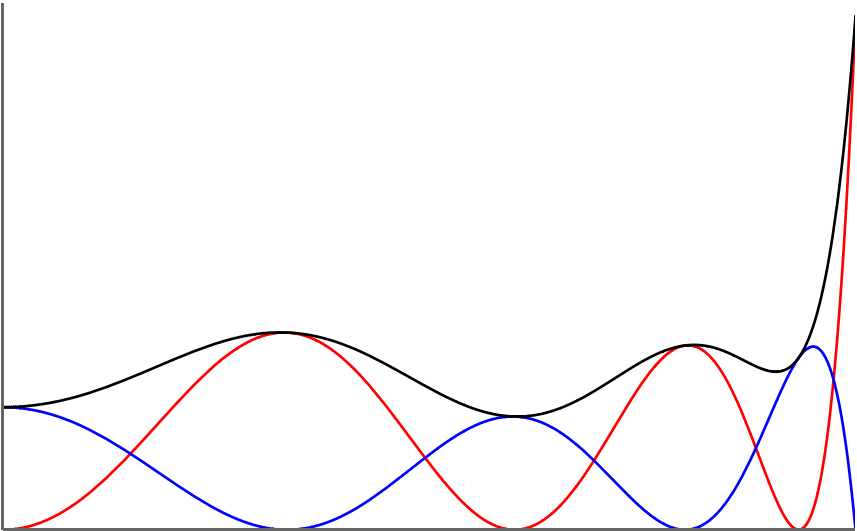
(a) $n=5$

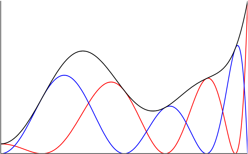
(b) $n=6$

Figure 1: The functions $f\in\mathcal{C}([a,b],\mathds{R})$ with $f>0$ (black), $f_{*}\in\mathrm{lin}\,\mathcal{F}$ (red), and $f^{*}\in\mathrm{lin}\,\mathcal{F}$ (blue) from the 3 with $n=5$ and $n=6$.

The proof is taken from (KS, 66, pp. 68–71). The proof constructs the polynomials $f_{*}$ and $f^{*}$ by using the Fixed Point Theorem of Brouwer (Bro, 11, Satz 4), see also e.g. (Zei, 86, Prop. 2.6).

Proof 35.1.

We distinguish three different cases.

Case 1: Let $n=2m$ and let $\mathcal{F}$ be an ET-system. We construct $f_{*}$ in (i) as follows. For each point $\xi=(\xi_{0},\dots,\xi_{m})$ in the $m$-dimensional simplex

$$\Xi^{m}:=\left\{(\xi_{0},\dots,\xi_{m})\in\mathds{R}^{m+1}\,\middle|\,\xi_{i}\geq 0,\ i=0,1,\dots,m,\ \sum_{i=0}^{m}\xi_{i}=b-a\right\}$$ (54)

set

$$x_{i}:=a+\sum_{k=0}^{i-1}\xi_{k}$$

for all $i=0,\dots,m$ and define

$$f_{\xi}(x):=c_{\xi}\cdot\det\left(\begin{array}[]{c|ccccc}f_{0}&\,f_{1}&f_{2}&\dots&f_{n-1}&f_{n}\\ x&\,x_{1}&x_{1}&\dots&x_{m}&x_{m}\end{array}\right)$$ (55)

with $c_{\xi}\in\mathds{R}$ such that $f_{\xi}=\sum_{i=0}^{n}a_{i}f_{i}\geq 0$ on $[a,b]$ with $a_{0}^{2}+\dots+a_{n}^{2}=1$. If $p$ of the points $x_{i}$ coincide, this common point is to have multiplicity $2p$.

Define

$$\delta_{i}(\xi):=\min\{\delta\geq 0\,|\,\delta\cdot f\geq u_{\xi}\ \text{on}\ [x_{i},x_{i+1}]\}$$ (56)

for all $i=0,\dots,m$ with $x_{0}=a$ and $x_{m+1}=b$. The coefficients $a_{i}(\xi)$ are continuous in $\xi$ and hence the functions $\delta_{i}(\xi)$ are continuous in $\xi$.

Next, define

$$F_{i}(\xi):=\delta_{i}(\xi)-\min_{k}\delta_{k}(\xi)$$ (57)

for all $i=0,\dots,m$ and set $F_{m+1}(\xi):=F_{0}(\xi)$. If there does not exist a point $\xi$ such that $F_{i}(\xi)=0$ for all $i=0,\dots,m$, then $\sum_{i=0}^{m}F_{i}(\xi)>0$ for all $\xi\in\Xi^{m}$. In this event the continuous mapping

$$\cdot\,^{\prime}:\Xi^{m}\to\Xi^{m},\ \xi\mapsto\xi^{\prime}\quad\text{with}\quad\xi_{i}^{\prime}:=\frac{F_{i+1}(\xi)}{\sum_{k=0}^{m}F_{k}(\xi)}\cdot(b-a)$$

for all $i=0,\dots,m$ is well-defined. The Fixed Point Theorem of Brouwer affirms the existence of a point $\xi^{*}\in\Xi^{m}$ for which

$$\xi_{i}^{*}:=\frac{F_{i+1}(\xi^{*})}{\sum_{k=0}^{m}F_{k}(\xi^{*})}\cdot(b-a)$$ (58)

for all $i=0,\dots,m$. By (57) we have that for any $\xi\in\Xi^{m}$ we have $F_{i}(\xi)=0$ for some $i$. Suppose $F_{j}(\xi^{*})=0$ for some fixed $j=0,\dots,m$. Then (58) implies $\xi_{j-1}^{*}=0$. By (56) and (57) imply $F_{j-1}(\xi^{*})=0$. Continuing in this way we get $F_{i}(\xi^{*})=0$ for all $i=0,\dots,j$ and since $F_{m+1}(\xi)=F_{0}(\xi)$ we have $F_{i}(\xi^{*})=0$ for all $i=0,\dots,m$. But this contradicts our assumption $\sum_{i=0}^{m}F_{i}(\xi^{*})>0$. Therefore, there exists at least one point $\xi^{*}\in\Xi^{m}$ such that $\delta_{i}(\xi^{*})=\delta$ for all $i=0,\dots,m$. Since $f_{\xi}\neq 0$ it follows that $\delta>0$ and hence all $x_{i}$ are distinct, i.e.,

$$a=x_{0}<x_{1}<\dots<x_{m}=b.$$

Hence, $f_{*}:=\delta^{-1}\cdot f_{\xi^{*}}$ by the nature of its construction fulfills the requirements (a) – (e) of (i).

For $f^{*}$ we let $x_{0}=a$ and $x_{m}=b$ and we define similar to (55) the polynomial

$$g_{\xi}(x):=d_{\xi}\cdot\det\left(\begin{array}[]{c|ccccccc}f_{0}&\,f_{1}&f_{2}&f_{3}&\dots&f_{n-2}&f_{n-1}&f_{n}\\ x&\,a&x_{1}&x_{1}&\dots&x_{m-1}&x_{m-1}&b\end{array}\right).$$

Repeating the arguments from above we get $f^{*}$ which fulfills (a) – (d) and (e’) in (ii).

Case 2: Let $n=2m+1$ and let $\mathcal{F}$ be an ET-system. Similar to case 1, we define the polynomials

$$f_{\xi}(x):=d_{\xi}\cdot\det\left(\begin{array}[]{c|cccccc}f_{0}&\,f_{1}&f_{2}&f_{3}&\dots&f_{n-1}&f_{n}\\ x&\,a&x_{1}&x_{1}&\dots&x_{m}&x_{m}\end{array}\right).$$

and

$$g_{\xi}(x):=d_{\xi}\cdot\det\left(\begin{array}[]{c|cccccc}f_{0}&\,f_{1}&f_{2}&\dots&f_{n-2}&f_{n-1}&f_{n}\\ x&\,x_{1}&x_{1}&\dots&x_{m}&x_{m}&b\end{array}\right).$$

Repeating the procedure of case 1 gives the statement.

Case 3: Let $n=2m$ and $\mathcal{F}$ be a T-systems. Then we consider the functions

$$f_{i}(x;\sigma):=\int_{a}^{b}K_{\sigma}(x,y)\cdot f_{i}(y)~{}\mathrm{d}y$$

where

$$K_{\sigma}(x,y):=\frac{1}{\sigma\cdot\sqrt{2\pi}}\exp\left[-\frac{1}{2}\left(\frac{x-y}{\sigma}\right)^{2}\right]$$

with $\sigma>0$, see Chapter 6. By 8 we have that $\mathcal{F}_{\sigma}:=\{f_{i}(\,\cdot\,;\sigma)\}_{i=0}^{n}$ is an ET-system on $[a,b]$ and hence also on any subinterval $[a^{\prime},b^{\prime}]$ with $a<a^{\prime}<b^{\prime}<b$. The need to restrict the system $\mathcal{F}_{\sigma}$ to the proper interval $[a^{\prime},b^{\prime}]$ is due to the annoyance that at the end points $x=a$ and $x=b$ we have

$$\lim_{\sigma\searrow 0}f_{i}(x;\sigma)=\frac{1}{2}f_{i}(x)$$

for all $i=0,\dots,n$ while for $x\in(a,b)$ we have

$$\lim_{\sigma\searrow 0}f_{i}(x;\sigma)=f_{i}(x).$$

From the cases 1 and 2 we find that for any $\sigma>0$ we have a polynomial $f_{*,\sigma}$ satisfying conditions (a) – (e) of (i) on the interval $[a^{\prime},b^{\prime}]$. If

$$f_{*,\sigma}=\sum_{i=0}^{n}a_{i}(\sigma)\cdot f_{i}(\,\cdot\,,\sigma)$$

we can chose a sequence $\sigma_{k}\searrow 0$ and let $x_{1}^{(k)},\dots,x_{m}^{(k)}$ be the zeros of $f_{*,\sigma_{k}}$. Additionally, let $y_{1}^{(k)},\dots,y_{m+1}^{(k)}$ be the points which interlace with $\{x_{i}^{(k)}\}_{i=0}^{m}$, i.e., $a^{\prime}<y_{1}^{(k)}<x_{1}^{(k)}<\dots<x_{m}^{(k)}<y_{m+1}^{(k)}\leq b^{\prime}$ and satisfying $f(y_{i}^{(k)})=f_{*,\sigma_{k}}(y_{i}^{(k)})$ for all $i=0,\dots,m+1$.

Since $f(x)\geq f_{*,\sigma}\geq 0$ on $[a^{\prime},b^{\prime}]$ and solving the system of equations

$$f_{*,\sigma}(x_{j})=\sum_{i=0}^{n}a_{i}(\sigma)\cdot f_{i}(x_{j};\sigma)$$

for $i=0,\dots,n$ we find that these quantities are uniformly bounded. We now select a subsequence $\{\sigma_{k^{\prime}}\}$ from $\{\sigma_{k}\}$ with the property that as $k^{\prime}\to\infty$ we obtain

$$a_{i}(\sigma_{k^{\prime}}) \to a_{i} \text{for all}\ i=0,\dots,n,$$

$$y_{j}^{(k^{\prime})} \to y_{j} \text{for all}\ j=1,\dots,m+1,$$

$$x_{l}^{(k^{\prime})} \to x_{l} \text{for all}\ l=1,\dots,m$$

and

$$a^{\prime}\leq y_{1}\leq x_{1}\leq\dots\leq x_{m}\leq y_{m+1}\leq b^{\prime}.$$

The function $f_{*,a^{\prime},b^{\prime}}:=\sum_{i=0}^{n}a_{i}\cdot f_{i}$ vanishes at all $x_{l}$, $l=1,\dots,m$, and equals $f$ at all $y_{j}$, $j=1,\dots,m+1$. Therefore, since $f_{*,a^{\prime},b^{\prime}}$ is continuous we see that

$$a^{\prime}\leq y_{1}<x_{1}<\dots<x_{m}<y_{m+1}\leq b^{\prime}.$$

Hence, $f_{*,a^{\prime},b^{\prime}}$ satisfies (a) – (e) of (i) on the interval $[a^{\prime},b^{\prime}]$.

Performing a last limiting procedure letting $a^{\prime}\searrow a$ and $b^{\prime}\nearrow b$ we obtain a polynomial $f_{*}$ satisfying (a) – (e) in (i) on the full interval $[a,b]$.

For $f^{*}$ the same procedure gives the desired polynomial satisfying the conditions (a) – (d) and (e’).

Uniqueness of $f_{*}$ and $f^{*}$: Let $n=2m$. Observe that if another polynomial $\tilde{f}_{*}$ with properties (a) – (e) exists then it must have $m$ interior zeros $\tilde{x}_{1},\dots,\tilde{x}_{m}$. Denote by $x_{1},\dots,x_{m}$ the zeros of $f_{*}$. Without loss of generality we can assume that either $\tilde{x}_{1}<x_{1}$ or $\tilde{x}_{1}=x_{1}$ and $f_{*}-\tilde{f}_{*}$ is non-negative in some interval $(x_{1}-\varepsilon,x_{1})$. Otherwise we interchange the roles of $f_{*}$ and $\tilde{f}_{*}$. We count the zeros of $g:=f_{*}-\tilde{f}_{*}$. We say $g$ has a zero in the closed interval $[c,d]$ if

• $g(t_{0})=0$ for $t_{0}\in(c,d)$,

• $g(c)=0$ and $g\geq 0$ on $(c,c+\varepsilon)$, or

• $g(d)=0$ and $g\geq 0$ on $(d-\varepsilon,d)$.

Counting zeros in this fashion we see that $g$ has at least two zeros in each of the intervals $[x_{i-1},x_{i}]$ for $i=1,\dots,m$ where $x_{0}=a$ and at least one in the interval $[x_{m},b]$. In total $g$ vanishes at least $n+1$ times. Notice, that certain non-nodal zeros of $g$ have been counted twice and hence by 22 we have $g=0$.

In a similar way we get uniqueness of $f^{*}$ and also in the case $n=2m+1$.

Note, in the previous result we do not need to have $f\in\mathrm{lin}\,\mathcal{F}$. The function $f$ only needs to be continuous and strictly positive on $[a,b]$.

An earlier version of (or at least connected to) 1 combined with 22 (which was used in the proof of 1) is a lemma by Markov Mar (84), see also (ST, 43, p. 80).

Lemma 2 (Mar (84), see also (ST, 43, p. 80)).

Let $m\in\mathds{N}$ and let $f\in\mathcal{C}^{n+1}([a,b],\mathds{R})$ be such that $f>0$ and $f^{(k)}\geq 0$ for all $k=1,\dots,m+1$ in $[a,b]$. Let $p_{m}\in\mathds{R}[x]_{\leq m}$ and $c\in(a,b)$. Let $m_{1}\in\mathds{N}$ be the number of zeros in $(a,c)$ of the function $f-p_{m}$ and $m_{2}$ be the number of zeros of $p_{m}$ in $(c,b)$, both counted with multiplicity. Then $m_{1}+m_{2}\leq m+1$.

1 is of course much more general. As a consequence of 1 we get Karlin’s Positivstellensatz for T-systems on $[a,b]$.

Karlin’s Positivstellensatz 3 (for T-Systems on $[a,b]$; see (Kar, 63, Cor. 1) or e.g. (KS, 66, p. 71, Cor. 10.1(a))).

Let $n\in\mathds{N}_{0}$, let $\mathcal{F}$ be a continuous T-system of order $n$ on $[a,b]$ with $a<b$, and let $f\in\mathrm{lin}\,\mathcal{F}$ with $f>0$ on $[a,b]$. Then there exists a unique representation

$$f=f_{*}+f^{*}$$

with $f_{*},f^{*}\in\mathrm{lin}\,\mathcal{F}$ such that

1. $f_{*},f^{*}\geq 0$ on $[a,b]$,

2. the zeros of $f_{*}$ and $f^{*}$ each are sets of index $n$,

3. the zeros of $f_{*}$ and $f^{*}$ strictly interlace,

4. $f_{*}(b)=f(b)>0$, and

5. $f^{*}(b)=0$.

Proof 35.2.

Let $f_{*}$ be the unique $f_{*}$ from 1(i). Then $f-f_{*}\in\mathrm{lin}\,\mathcal{F}$ is a polynomial and fulfills (a) – (d), and (e’) of $f^{*}$ in 1. But since also $f^{*}$ is unique we have $f-f_{*}=f^{*}$.

36 The Snake Theorem: An Interlacing Theorem

In 1 a polynomial $f_{*}\in\mathrm{lin}\,\mathcal{F}$ was found with $0\leq f_{*}\leq f$ for some given $f\in\mathcal{C}([a,b],\mathds{R})$ with $f>0$ on $[a,b]$. This can be extended to find a function $f_{*}\in\mathrm{lin}\,\mathcal{F}$ between some $g_{1},g_{2}\in\mathcal{C}([a,b],\mathds{R})$ as the following result shows. In (KS, 66, p. 368, Thm. 6.1) M. G. Krein and A. A. Nudel’man called it the Snake Theorem which is an accurate description of its graphical representation, see Figure 2.

Snake Theorem 4 ((Kar, 63, Thm. 2) or e.g. (KS, 66, p. 72, Thm. 10.2) and (KN, 77, p. 368, Thm. 6.1)).

Let $n\in\mathds{N}_{0}$, $\mathcal{F}=\{f_{i}\}_{i=0}^{n}$ be a continuous T-system of order $n$ on $[a,b]$ with $a<b$, and let $g_{1},g_{2}\in\mathcal{C}([a,b],\mathds{R})$ be two continuous functions on $[a,b]$ such that there exists a function $g\in\mathrm{lin}\,\mathcal{F}$ with

$$g_{1}<g<g_{2}$$

on $[a,b]$. Then the following hold:

1. There exists a unique polynomial $f_{*}\in\mathrm{lin}\,\mathcal{F}$ such that

   1. $g_{1}(x)\leq f_{*}(x)\leq g_{2}(x)$ for all $x\in[a,b]$, and

   2. there exist $n+1$ points $x_{1}<\dots<x_{n+1}$ in $[a,b]$ such that

      $$f_{*}(x_{n+1-i})=\begin{cases}g_{1}(x_{n+1-i})&\text{for}\ i=1,3,5,\dots,\\ g_{2}(x_{n+1-i})&\text{for}\ i=0,2,4,\dots.\end{cases}$$

2. There exists a unique polynomial $f^{*}\in\mathrm{lin}\,\mathcal{F}$ such that

   1. $g_{1}(x)\leq f^{*}(x)\leq g_{2}(x)$ for all $x\in[a,b]$, and

   2. there exist $n+1$ points $y_{1}<\dots<y_{n+1}$ in $[a,b]$ such that

      $$f^{*}(y_{n+1-i})=\begin{cases}g_{2}(y_{n+1-i})&\text{for}\ i=1,3,5,\dots,\\ g_{1}(y_{n+1-i})&\text{for}\ i=0,2,4,\dots.\end{cases}$$

The functions $g_{1}$, $g_{2}$, $g$, $f_{*}$, and $f^{*}$ of the 4 are illustrated in Figure 2.

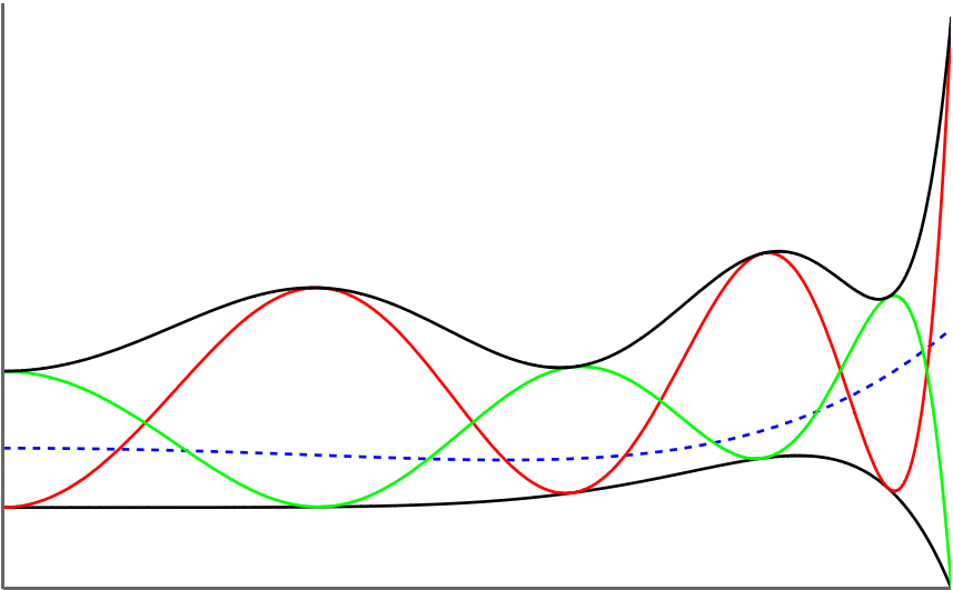
Figure 2: The functions $g_{1},g_{2}\in\mathcal{C}([a,b],\mathds{R})$ (black, $g_{1}$ bottom, $g_{2}$ top), $g\in\mathrm{lin}\,\mathcal{F}$ (blue, dashed), $f_{*}\in\mathrm{lin}\,\mathcal{F}$ (red), and $f^{*}\in\mathrm{lin}\,\mathcal{F}$ (green) from the 4.

The following proof is taken from (KS, 66, p. 73).

Proof 36.1.

Let $n=2m$ and $\mathcal{F}$ be an ET-system. We proceed as in the proof of 1. For each $\xi=(\xi_{0},\dots,\xi_{n})\in\Xi^{n}$ and $\sum_{i=0}^{n}\xi_{i}=b-a$ we construct the polynomial

$$f_{\xi}(x)=\sum_{i=0}^{n}a_{i}(\xi)\cdot f_{i}(x)=c_{\xi}\cdot\det\left(\begin{array}[]{c|ccc}f_{0}&\,f_{1}&\dots&f_{n}\\ x&\,x_{1}&\dots&x_{n}\end{array}\right)$$

which vanishes at each of the points

$$x_{i}:=a+\sum_{k=0}^{i-1}\xi_{k}$$

for all $i=0,\dots,n$ and let $c_{\xi}\in\mathds{R}$ be such that $a_{0}(\xi)^{2}+\dots+a_{n}(\xi)^{2}=1$ and $f_{\xi}\geq 0$ on $[x_{i},x_{i+1}]$ if $i$ is even.

For $i=0,2,4,\dots,n$ we define

$$\delta_{i}(\xi):=\min\left\{\delta\geq 0\,\middle|\,\delta\cdot(g_{2}-g)\geq f_{\xi}\ \text{on}\ [x_{i},x_{i+1}]\right\},$$

where $x_{0}=a$ and $x_{n+1}=b$, while for $i=1,3,\dots,n-1$ we define

$$\delta_{i}(\xi):=\min\left\{\delta\geq 0\,\middle|\,f_{\xi}\geq\delta\cdot(g-g_{1})\ \text{on}\ [x_{i},x_{i+1}]\right\}.$$

As in 1 we define $F_{k}(\xi):=\delta_{k}(\xi)-\min_{i}\delta_{i}(\xi)$. And as before assuming $\sum_{k=0}^{n}F_{k}(\xi)>0$ for all $\xi\in\Xi^{n}$ leads to a contradiction. Therefore, there exists a $\xi^{*}\in\Xi^{n}$ for which $\delta_{i}(\xi^{*})=\delta$ for all $i=0,\dots,n$. It is clear that $\delta>0$ and that the polynomial $f_{*}:=\delta^{-1}\cdot f_{\xi^{*}}+g$ satisfies the conditions of the theorem.

The polynomial $f^{*}$ is constructed employing the same line of arguments.

The extension encompassing the case where $\mathcal{F}$ is merely a T-system and the proof of the uniqueness proceed as in the proof of 1.

37 Karlin’s Nichtnegativstellensatz for ET-Systems on $[a,b]$

While 1 with $f>0$ can be proved for T-systems, an equivalent version allowing zeros in $f\in\mathcal{C}([a,b],\mathds{R})$, i.e., $f\geq 0$ but not $f>0$, needs to assume that $\mathcal{F}$ is an ET-system.

Karlin’s Theorem 5 (for $f\geq 0$ on $[a,b]$; (Kar, 63, Thm. 3) or e.g. (KS, 66, p. 74, Thm. 10.3)).

Let $n\in\mathds{N}_{0}$, let $\mathcal{F}=\{f_{i}\}_{i=0}^{n}$ be a continuous ET-system of order $n$ on $[a,b]$ with $a<b$, and let $f\in\mathcal{C}^{n}([a,b],\mathds{R})$ be such that $f\geq 0$ on $[a,b]$ and $f$ has $r<n$ zeros (counting multiplicities). The following hold:

1. There exists a unique polynomial $f_{*}\in\mathrm{lin}\,\mathcal{F}$ such that

   1. $f(x)\geq f_{*}(x)\geq 0$ for all $x\in[a,b]$,

   2. $f_{*}$ has $n$ zeros counting multiplicities,

   3. if $x_{1}<\dots<x_{{n-r}}$ in $(a,b)$ are the zeros of $f_{*}$ which remain after removing the $r$ zeros of $f$ then $f-f_{*}$ vanishes at least twice more (counting multiplicities) in each open interval $(x_{i},x_{i+1})$, $i=1,\dots,n-r-1$, and at least once more in each of the intervals $[a,x_{1})$ and $(x_{n-r},b]$,

   4. the zeros $x_{1},\dots,x_{n-r}$ of (c) are a set of index $n-r$, and

   5. $x_{n-r}<b$.

2. There exists a unique polynomial $f^{*}\in\mathrm{lin}\,\mathcal{F}$ which satisfies the conditions (a) to (d) and

   1. $x_{n-r}=b$.

The proof is taken from (KS, 66, pp. 74–75).

Proof 37.1.

Let $z_{1},\dots,z_{p}$ be the distinct zeros of $f$ with multiplicities $m_{1},\dots,m_{p}$ where $\sum_{i=1}^{p}m_{i}=r\leq n-1$ and set $n^{\prime}:=n-r$. The proof is now similar to the proof of 1 where $n$ is replaced by $n^{\prime}$. Since the odd and the even cases are again somewhat the same and for the sake of some slight variety we treat now the odd case $n^{\prime}=2m^{\prime}+1$. The construction of $f_{*}$ in part (i) proceeds as follows. For each $\xi\in\Xi^{m^{\prime}}$ we construct the polynomial

$$f_{\xi}(x):=\sum_{i=0}^{n}a_{i}(\xi)\cdot f_{i}\\ =c_{\xi}\cdot\det\left(\begin{array}[]{c|cccccccc}f_{0}&\,f_{1}\dots f_{m_{1}}&\dots&f_{m_{1}+m_{p-1}+1}&\dots f_{r}&f_{r+1}\;f_{r+2}&\dots&f_{n-2}\;f_{n-1}&f_{n}\\ x&\,z_{1}\,\dots\,z_{1}&\dots&z_{p}&\dots\,z_{p}&x_{1}\;\;\;x_{1}&\dots&x_{n^{\prime}}\;\;\,x_{n^{\prime}}&a\end{array}\right)$$ (59)

where $c_{\xi}\in\mathds{R}$ is chosen such that $a_{1}(\xi)^{2}+\dots+a_{n}(\xi)^{2}=1$ and

$$x_{i}:=a+\sum_{k=0}^{i}\xi_{k}$$

for all $i=1,\dots,m^{\prime}$ are the zeros of multiplicity two and $a$ is a zero of multiplicity one. Now we define

$$\delta_{i}(\xi):=\min\left\{\delta\geq 0\,\middle|\,\delta\geq\frac{f_{\xi}}{f}\ \text{on}\ [x_{i},x_{i+1}]\right\}$$

for $i=1,\dots,m^{\prime}+1$ with $x_{m^{\prime}+2}=b$ where the ratio is evaluated by l’Hopital’s rule at the zeros $z_{1},\dots,z_{p}$ of $f$.

By examining $\frac{f_{\xi}}{f}$ first in the neighborhood of each of the points $z_{1},\dots,z_{p}$ and then over the remaining part we find that if $\xi^{(k)}\to\xi$ then

$$\frac{f_{\xi^{(k)}}}{f}\to\frac{f_{\xi}}{f}$$

uniformly on $[a,b]$. Consequently, each of th $\delta_{i}$ is continuous in $\xi$ and $\delta_{i}(\xi)=0$ if and only $\xi_{i}=0$.

The same arguments used in the proof of 1 now show that for some $\xi^{*}\in\mathrm{int}\,\Xi^{m^{\prime}}$ we have $\delta_{i}(\xi^{*})=\delta>0$ for all $i=1,\dots,m^{\prime}+1$. It is simple to see that $f_{*}:=\delta^{-1}\cdot f_{\xi^{*}}$ possesses the properties (a), (b), (d), and (e) in (i). To show property (c) observe that if $x_{i}=z_{j}$ for some $j$ then $f_{\xi^{*}}$ has a zero at $z_{j}$ with multiplicity exceeding that of $f$ so that $\delta$ is strictly greater than $f_{\xi^{*}}\cdot f^{-1}$ in some neighborhood of $z_{j}$. This implies the equality $\delta=f_{\xi^{*}}(x)\cdot f(x)^{-1}$ for some $x$ in each of the open intervals $(x_{1},x_{2})$, …, $(x_{m^{\prime}},x_{m^{\prime}+1})$ and somewhere in $(x_{m^{\prime}+1},b]$. Thus, in each $(x_{i},x_{i+1})$, either $f(x)-\delta^{-1}\cdot f_{\xi^{*}}(x)$ vanishes somewhere other than at the zeros of $f$ or the multiplicity of one of the common zeros of $f$ and $\delta^{-1}\cdot f_{\xi^{*}}$ is increased by two. In the interval $(x_{m^{\prime}+1},b]$ the function $f-\delta^{-1}\cdot f_{\xi}$ may vanish at $b$ with multiplicity only one greater than the zero of $f$ at this point. This concludes that $f_{*}$ also fulfills (c) in (i).

The polynomial $f^{*}$ when $n^{\prime}=2m^{\prime}+1$ is constructed in the same manner by replacing $a$ in (59) by $b$.

Uniqueness: Assume another polynomial $g$ satisfies the same properties as $f_{*}$. Without loss of generality we can assume that the first zero of $f-g$ other than the zeros of $f$ is less than or equal to first zero of $f-f_{*}$. Define $h:=\frac{f_{*}-g}{f}$. A zero of $h$ occurring at one of the values $x_{i}$, $i=2,\dots,n^{\prime}+1$ is necessarily at least a double zero. In this case we assign one zero to each of the intervals $[x_{i-1},x_{i}]$ and $[x_{i},x_{i+1}]$ with $x_{m^{\prime}+2}=b$. Under this counting procedure, and taking account of the oscillation properties of $f_{*}$ and $g$, we deduce that $h$ has at least three zeros in $[a,x_{1}]$, at least two zeros in each of the intervals $[x_{i},x_{i+1}]$, $i=2,\dots,m^{\prime}$, and at least one zero in $[x_{m^{\prime}+1},b]$. Clearly, all of these zeros are other than the $r$ zeros of $f$, so that $f_{*}-g$ has at least $3+2(m^{\prime}-1)+1+r=n+1$ zeros (counting multiplicities). Hence, $h=0$ and $f_{*}=g$.

If $f\in\mathrm{lin}\,\mathcal{F}$ in 5 we get similar to 3 the following Nichtnegativstellensatz on $[a,b]$ due to Karlin.

Karlin’s Nichtnegativstellensatz 6 (for ET-Systems on $[a,b]$; (Kar, 63, p. 603, Cor. after Thm. 3) or e.g. (KS, 66, p. 76, Cor. 10.3)).

Let $n\in\mathds{N}_{0}$, $\mathcal{F}=\{f_{i}\}_{i=0}^{n}$ be an ET-system of order $n$ on $[a,b]$ with $a<b$, and let $f\in\mathrm{lin}\,\mathcal{F}$ be such that $f\geq 0$ on $[a,b]$ and $f$ has $r<n$ zeros $a\leq z_{1}\leq z_{2}\leq\dots\leq z_{r}\leq b$ (counting multiplicities). Then there exists a unique representation

$$f=f_{*}+f^{*}$$

with $f_{*},f^{*}\in\mathrm{lin}\,\mathcal{F}$ such that

1. $f_{*},f^{*}\geq 0$ on $[a,b]$,

2. for $f_{*}$ and $f^{*}$ the sets of zeros counting algebraic multiplicities is after removing the zeros of $f$ with algebraic multiplicity a set of index $n-r$ which strictly interlace, and

3. the set of zeros of $f^{*}$ contains after removing the zeros of $f$ with algebraic multiplicities the point $b$.

Proof 37.2.

Let $f_{*}$ be the polynomial from 5 and set $g:=f-f_{*}$. Then $g$ fulfills the conditions of $f^{*}$ in 5 and by its uniqueness we have $g=f^{*}$ which proves the statement.

Remark 7.

Since 6 (ii) might be a little bit confusing we explain it more detailed.

Let $\mathcal{F}$ be an ET-system of order $n\in\mathds{N}_{0}$ on $[a,b]$ with $a<b$ and let $f\in\mathrm{lin}\,\mathcal{F}$ be such that $f\geq 0$ on $[a,b]$ and $f$ has the zeros $z_{1},\dots,z_{l}$ with algebraic multiplicities $m_{1},\dots,m_{l}$, $m_{1}+\dots+m_{l}=:r<n$.

1. If $n-r=2m$ is even then the zeros of $f_{*}$ from 6 are $x_{1},\dots,x_{m}$ all with algebraic multiplicity $2$ and the zeros of $f^{*}$ are $y_{0},y_{1},\dots,y_{m}$ where $y_{0}$ and $y_{m}$ have algebraic multiplicity $1$ and otherwise the $y_{i}$ have algebraic multiplicity $2$. They interlace, i.e., we have

   $$a=y_{0}<x_{1}<y_{1}<\dots<x_{m}<y_{m}=b.$$

   The $f_{*}$ and $f^{*}$ are then given by

   $$f_{*}(x)=c_{*}\cdot\det\left(\begin{array}[]{c|cccccccc}f_{0}&\,f_{1}&f_{2}&\dots&f_{2m-1}&f_{2m}&f_{2m+1}&\dots&f_{n}\\ x&\,x_{1}&x_{1}&\dots&x_{m}&x_{m}&z_{1}&\dots&z_{l}\end{array}\right)$$

   and

   $$f^{*}(x)=c^{*}\cdot\det\left(\begin{array}[]{c|ccccccccc}f_{0}&\,f_{1}&f_{2}\;f_{3}\dots&f_{2m-2}&f_{2m-1}&f_{2m}&f_{2m+1}&\dots&f_{n}\\ x&\,a&y_{1}\;y_{1}\dots&y_{m-1}&y_{m-1}&b&z_{1}&\dots&z_{l}\end{array}\right)$$

   where $c_{*},c^{*}\in\mathds{R}\setminus\{0\}$ and the signs are such that $f_{*},f^{*}\geq 0$ on $[a,b]$. The zeros $z_{1},\dots,z_{l}$ are included with their corresponding algebraic multiplicities $m_{1},\dots,m_{l}$, i.e., $z_{1}$ is included $m_{1}$-times, …, $z_{l}$ is included $m_{l}$-times.

2. If $n-r=2m+1$ is odd then the zeros of $f_{*}$ from 6 are $x_{0},\dots,x_{m}$ where $x_{0}$ has algebraic multiplicity $1$ and the other algebraic multiplicity $2$. For $f^{*}$ we have the zeros $y_{0},\dots,y_{m}$ where $y_{0},\dots,y_{m-1}$ have algebraic multiplicity $2$ and $y_{m}$ has algebraic multiplicity $1$. They interlace, i.e., we have

   $$x_{0}=a<y_{0}<\dots<x_{m}<y_{m}=b.$$

   The $f_{*}$ and $f^{*}$ are then given by

   $$f_{*}(x)=c_{*}\cdot\det\left(\begin{array}[]{c|ccccccccc}f_{0}&\,f_{1}&f_{2}\;f_{3}\dots&f_{2m}&f_{2m+1}&f_{2m+2}&\dots&f_{n}\\ x&\,a&x_{1}\;x_{1}\dots&x_{m}&x_{m}&z_{1}&\dots&z_{l}\end{array}\right)$$

   and

   $$f^{*}(x)=c^{*}\cdot\det\left(\begin{array}[]{c|cccccccc}f_{0}&\,f_{1}\;f_{2}&\dots&f_{2m-1}&f_{2m}&f_{2m+1}&f_{2m+2}&\dots&f_{n}\\ x&\,y_{0}\;y_{0}&\dots&y_{m-1}&y_{m-1}&b&z_{1}&\dots&z_{l}\end{array}\right)$$

   where $c_{*},c^{*}\in\mathds{R}\setminus\{0\}$ and the signs are such that $f_{*},f^{*}\geq 0$ on $[a,b]$. The zeros $z_{1},\dots,z_{l}$ are included with their corresponding algebraic multiplicities $m_{1},\dots,m_{l}$, i.e., $z_{1}$ is included $m_{1}$-times, …, $z_{l}$ is included $m_{l}$-times. $\circ$

With the proof of 5 one can prove a similar interlacing theorem as the 4 when $g_{2}-g_{1}$ has a certain number of zeros, see (KS, 66, p. 76, Rem. 10.1).

We stated here 3 and 6 for functions on $[a,b]$. There are also similar statements for periodic functions, see (Kar, 63, Thm. 6 and 7). The cases on $[0,\infty)$ and $\mathds{R}$ are given in the next chapter.

Problems

Problem 8.

Examine the proof of 5 more closely. In the statement of the theorem it is required that $\mathcal{F}$ is an ET-system on $[a,b]$. But for a given $f\geq 0$ where does the family $\mathcal{F}$ actually only needs to be an ET-system?

Look at the conclusion! And try to think of a familiar
theorem having the same or a similar conclusion.
           George Pólya (Pól, 45, p. 25)

Chapter 8 Karlin’s Positivstellensätze and Nichtnegativstellensätze on $[0,\infty)$ and $\mathds{R}$

In this chapter we extend the results of the previous chapter, i.e., we extend 3 on $[a,b]$ to $[0,\infty)$ in 1 and to $\mathds{R}$ in 4 as well as we extend 6 on $[a,b]$ to $[0,\infty)$ in 3 and to $\mathds{R}$ in 5.

38 Karlin’s Positivstellensatz for T-Systems on $[0,\infty)$

By a transformation of $[a,b]$ to $[0,\infty]$ and then restriction to $[0,\infty)$ we get from 3 the following.

Karlin’s Positivstellensatz 1 (for T-Systems on $[0,\infty)$; see (Kar, 63, Thm. 9) or e.g. (KS, 66, p. 169, Thm. 8.1)).

Let $n\in\mathds{N}_{0}$ and $\mathcal{F}=\{f_{i}\}_{i=0}^{n}$ be a continuous T-system of order $n$ on $[0,\infty)$ such that

1. there exists a $C>0$ such that $f_{n}(x)>0$ for all $x\geq C$,

2. $\displaystyle\lim_{x\to\infty}\frac{f_{i}(x)}{f_{n}(x)}=0$ for all $i=0,\dots,n-1$, and

3. $\{f_{i}\}_{i=0}^{n-1}$ is a continuous T-system on $[0,\infty)$.

Then for any $f=\sum_{i=0}^{n}a_{i}f_{i}\in\mathrm{lin}\,\mathcal{F}$ with $f>0$ on $[0,\infty)$ and $a_{n}>0$ there exists a unique representation

$$f=f_{*}+f^{*}$$

with $f_{*},f^{*}\in\mathrm{lin}\,\mathcal{F}$ and $f_{*},f^{*}\geq 0$ on $[0,\infty)$ such that the following hold:

1. If $n=2m$ the polynomials $f_{*}$ and $f^{*}$ each possess $m$ distinct zeros $\{x_{i}\}_{i=1}^{m}$ and $\{y_{i}\}_{i=0}^{m-1}$ satisfying

   $$0=y_{0}<x_{1}<y_{1}<\dots<y_{m-1}<x_{m}<\infty.$$

   All zeros except $y_{0}$ are double zeros.

2. If $n=2m+1$ the polynomials $f_{*}$ and $f^{*}$ each possess the zeros $\{x_{i}\}_{i=1}^{m+1}$ and $\{y_{i}\}_{i=1}^{m}$ satisfying

   $$0=x_{1}<y_{1}<x_{2}<\dots<y_{m}<x_{m+1}<\infty.$$

   All zeros except $x_{1}$ are double zeros.

3. The coefficient of $f_{n}$ in $f_{*}$ is equal to $a_{n}$.

The proof is adapted from (KS, 66, pp. 168).

Proof 38.1.

By (a) there exists a function $w\in\mathcal{C}([0,\infty),\mathds{R})$ such that $w>0$ on $[0,\infty)$ and $\lim_{x\to\infty}\frac{f_{n}(x)}{w(x)}=1$. By (b) we define

$$v_{i}(x):=\begin{cases}\frac{f_{i}(x)}{w(x)}&\text{if}\ x\in[0,\infty),\\ \delta_{i,n}&\text{if}\ x=\infty\end{cases}$$

for all $i=0,1,\dots,n$. Then by (c) and 9 we have that $\{v_{i}\}_{i=0}^{n}$ is a T-system on $[0,\infty]$. With $t(x):=\tan(\pi x/2)$ we define $g_{i}(x):=v_{i}\circ t$ for all $i=0,1,\dots,n$. Hence, $\mathcal{G}=\{g_{i}\}_{i=0}^{n}$ is a T-system on $[0,1]$ by 8. We now apply 3 to $\mathcal{G}$. Set $g:=\big{(}\frac{f}{w}\big{)}\circ t$.

(i): Let $n=2m$. Then by 3 there exist points

$$0=y_{0}<x_{1}<y_{1}<\dots<x_{m}<y_{m}=1$$

and unique functions $g_{*}$ and $g^{*}$ such that $g=g_{*}+g^{*}$, $g_{*},g^{*}\geq 0$ on $[0,1]$, $x_{1},\dots,x_{m}$ are the zeros of $g_{*}$, and $y_{0},\dots,y_{m}$ are the zeros of $g^{*}$. Then $f_{*}:=(g_{*}\circ t^{-1})\cdot w$ and $f^{*}:=(g^{*}\circ t^{-1})\cdot w$ are the unique components in the decomposition $f=f_{*}+f^{*}$.

(ii): Similar to (i).

(iii): From (i) (and (ii) in a similar way) we have $g_{i}(1)=0$ for $i=0,\dots,n-1$ and $g_{n}(1)=1$. Hence, we get with $g^{*}(y_{m}=1)=0$ that $g_{n}$ is not contained in $g^{*}$, i.e., $g_{*}$ has the only $g_{n}$ contribution because $\mathcal{G}$ is linearly independent. This is inherited by $f_{*}$ and $f^{*}$ which proves (iii).

The transformation $g_{i}=v_{i}\circ t$ with $t$ the $\tan$-function is due to Krein Kre (51).

If $\mathcal{F}$ in 1 is an ET-system then the $f_{*}$ and $f^{*}$ can be written down explicitly. For that we only need $\mathcal{F}$ to be an ET-system on $(0,\infty)$ not on all $[0,\infty)$ since at $x=0$ a possible zero in $f_{*}$ or $f^{*}$ only has multiplicity one.

Corollary 2.

If in 1 we have additionally that $\mathcal{F}$ is an ET-system on $(0,\infty)$ then the unique $f_{*}$ and $f^{*}$ are given

1. for $n=2m$ by

   $$f_{*}(x)=c^{*}\cdot\det\begin{pmatrix}f_{0}&f_{1}&f_{2}&\dots&f_{2m-1}&f_{2m}\\ x&(x_{1}&x_{1})&\dots&(x_{m}&x_{m})\end{pmatrix}$$

   and

   $$f^{*}(x)=-c_{*}\cdot\det\begin{pmatrix}f_{0}&f_{1}&f_{2}&f_{3}&\dots&f_{2m-2}&f_{2m-1}\\ x&y_{0}&(y_{1}&y_{1})&\dots&(y_{m-1}&y_{m-1})\end{pmatrix},$$

2. and for $n=2m+1$ by

   $$f_{*}(x)=-c_{*}\cdot\det\begin{pmatrix}f_{0}&f_{1}&f_{2}&f_{3}&\dots&f_{2m}&f_{2m+1}\\ x&x_{1}&(x_{2}&x_{2})&\dots&(x_{m+1}&x_{m+1})\end{pmatrix}$$

   and

   $$f^{*}(x)=c^{*}\cdot\det\begin{pmatrix}f_{0}&f_{1}&f_{2}&\dots&f_{2m-1}&f_{2m}\\ x&(y_{1}&y_{1})&\dots&(y_{m}&y_{m})\end{pmatrix}$$

for some $c_{*},c^{*}>0$.

Proof 38.2.

Combine 1 with 28 and note that since $0$ is never a multiple zero we only need $\mathcal{F}$ to be an ET-system on $(0,\infty)$.

39 Karlin’s Nichtnegativstellensatz for ET-Systems on $[0,\infty)$

In 1 we needed to transform the domain $[a,b]$ into $[0,\infty]$ of a T-system. For 3 we needed an ET-system because of the additional zeros from $f\geq 0$.

With the same technique as in the proof of 1 and 8 we get from 6 the following.

Karlin’s Nichtnegativstellensatz 3 (for ET-Systems on $[0,\infty)$).

Let $n\in\mathds{N}_{0}$ and $\mathcal{F}=\{f_{i}\}_{i=0}^{n}$ be an ET-system of order $n$ on $[0,\infty)$ such that

1. there exists a $C>0$ such that $f_{n}(x)>0$ for all $x\geq 0$,

2. $\displaystyle\lim_{x\to\infty}\frac{f_{i}(x)}{f_{n}(x)}=0$ for all $i=0,\dots,n-1$, and

3. $\{f_{i}\}_{i=0}^{n-1}$ is an ET-system.

Then for any $f=\sum_{i=0}^{n}a_{i}f_{i}\in\mathrm{lin}\,\mathcal{F}$ such that $f\geq 0$ on $[0,\infty)$, $a_{n}>0$, and $f$ has $r<n$ zeros counting multiplicity there exists a unique representation

$$f=f_{*}+f^{*}$$

with $f_{*},f^{*}\in\mathrm{lin}\,\mathcal{F}$ such that the following hold:

1. $f_{*},\ f^{*}\geq 0$ on $[0,\infty)$,

2. $f_{*}$ has $n$ zeros (counting multiplicities),

3. $f^{*}$ has $n-1$ zeros (counting multiplicities),

4. the zeros of $f_{*}$ and $f^{*}$ strictly interlace if the zeros of $f$ are removed, and

5. the coefficient of $f_{n}$ in $f_{*}$ is equal to $a_{n}$.

Proof 39.1.

The conditions (a) – (c) are such that $\mathcal{F}$ on $[0,\infty]$, i.e., including $\infty$, is an ET-system.

With the same argument as in the proof of 1 we transform $\mathcal{F}$ on $[0,\infty]$ into $\mathcal{G}$ on $[0,1]$ with the $\tan$-function. Here 8 ensures that also $\mathcal{G}$ is an ET-system.

Application of 6 on $[0,1]$ gives the desired decomposition $g=g_{*}+g^{*}$ with the observation that $x=1$ is a zero of at most multiplicity one by (a) and (b). Backwards transformation into $\mathcal{F}$ on $[0,\infty]$ resp. $[0,\infty)$ then gives the assertion.

40 Karlin’s Positivstellensatz for T-Systems on $\mathds{R}$

We have seen that from 3 on $[a,b]$ we get 1 on $[0,\infty)$ with the transformation $t(x)=\tan(\pi x/2)$ from $[0,1]$ to $[0,\infty]$ and only need to pay attention to the end point $x=1$ resp. $x=\infty$. The same transformation however also applies going from $[-1,1]$ to $[-\infty,\infty]$ now paying attention to both end points.

Karlin’s Positivstellensatz 4 (for T-Systems on $\mathds{R}$; see (Kar, 63, Thm. 10) or e.g. (KS, 66, p. 198, Thm. 8.1)).

Let $m\in\mathds{N}_{0}$ and $\mathcal{F}=\{f_{i}\}_{i=0}^{2m}$ be a continuous T-system of order $2m$ on $\mathds{R}$ such that

1. there exists a $C>0$ such that $f_{2m}(x)>0$ for all $x\in(-\infty,-C]\cup[C,\infty)$,

2. $\displaystyle\lim_{|x|\to\infty}\frac{f_{i}(x)}{f_{2m}(x)}=0$ for all $i=0,\dots,2m-1$, and

3. $\{f_{i}\}_{i=0}^{2m-1}$ is a continuous T-system of order $2m-1$ on $\mathds{R}$.

Let $f=\sum_{i=0}^{2m}a_{i}f_{i}$ be such that $f>0$ on $\mathds{R}$ and $a_{2m}>0$. Then there exists a unique representation

$$f=f_{*}+f^{*}$$

with $f_{*},f^{*}\in\mathrm{lin}\,\mathcal{F}$ and $f_{*},f^{*}\geq 0$ on $\mathds{R}$ such that

1. the coefficient of $f_{2m}$ in $f_{*}$ is $a_{2m}$, and

2. $f_{*}$ and $f^{*}$ are non-negative polynomials having zeros $\{x_{i}\}_{i=1}^{m}$ and $\{y_{i}\}_{i=1}^{m-1}$ with

   $$-\infty<x_{1}<y_{1}<x_{2}<\dots<y_{m-1}<x_{m}<\infty.$$

Proof 40.1.

See Problem 6.

41 Karlin’s Nichtnegativstellensatz for ET-Systems on $\mathds{R}$

On $\mathds{R}$ we have the following Nichtnegativstellensatz for ET-systems.

Karlin’s Nichtnegativstellensatz 5 (for ET-Systems on $\mathds{R}$).

Let $m\in\mathds{N}_{0}$ and $\mathcal{F}=\{f_{i}\}_{i=0}^{2m}$ be an ET-system of order $2m$ on $\mathds{R}$ such that

1. there exists a $C>0$ such that $f_{2m}>0$ for all $x\in(-\infty,-C]\cup[C,\infty)$,

2. $\displaystyle\lim_{|x|\to\infty}\frac{f_{i}(x)}{f_{2m}(x)}=0$ for all $i=0,\dots,2m-1$,

3. $\{f_{i}\}_{i=0}^{n-1}$ is an ET-system of order $n-1$ on $\mathds{R}$.

Let $f=\sum_{i=0}^{2m}a_{i}f_{i}\in\mathrm{lin}\,\mathcal{F}$ be such that $f\geq 0$, $a_{2m}>0$, and $f$ has $r<n$ zeros counting multiplicities. Then there exists a unique representation

$$f=f_{*}+f^{*}$$

with $f_{*},f^{*}\in\mathrm{lin}\,\mathcal{F}$ such that the following hold:

1. $f_{*},f^{*}\geq 0$ on $\mathds{R}$,

2. $f_{*}$ has $2m$ zeros counting multiplicity,

3. $f^{*}$ has $2m-2$ zeros counting multiplicity,

4. the zeros of $f_{*}$ and $f^{*}$ strictly interlace if the zeros of $f$ are removed, and

5. the coefficient of $f_{n}$ in $f_{*}$ is equal to $a_{n}$.

Proof 41.1.

See Problem 7.

Problems

Problem 6.

Prove 4, i.e., adapt the proof of 1 such that both interval ends $a$ and $b$ of $[a,b]$ are mapped to $-\infty$ and $+\infty$, respectively.

Problem 7.

Prove 5, i.e., adapt the proof of 3 such that both interval ends $a$ and $b$ of $[a,b]$ are mapped to $-\infty$ and $+\infty$, respectively.

Part IV Non-Negative Algebraic Polynomials on $[a,b]$, $[0,\infty)$, and $\mathds{R}$

I hold that it is only when we can prove everything we assert
that we understand perfectly the thing under consideration.
           Gottfried Wilhelm Leibniz Lei (89)

Chapter 9 Non-Negative Algebraic Polynomials on $[a,b]$

We developed in the previous chapters the Positiv- and Nichtnegativestellensätze for general T- and ET-systems due to Karlin. We will now apply these to the algebraic polynomials, i.e., we will plug in 15 and 17.

42 Sparse Algebraic Positivstellensatz on $[a,b]$

At first let us have a look how all sparse strictly positive polynomials on some interval $[a,b]\subseteq(0,\infty)$ look like.

Theorem 1 (Sparse Algebraic Positivstellensatz on $[a,b]$ with $0<a<b$).

Let $n\in\mathds{N}_{0}$, $\alpha_{0},\dots,\alpha_{n}\in\mathds{R}$ be real numbers with $\alpha_{0}<\alpha_{1}<\dots<\alpha_{n}$, and let $\mathcal{F}=\{x^{\alpha_{i}}\}_{i=0}^{n}$. Then for any $f=\sum_{i=0}^{n}a_{i}x^{\alpha_{i}}\in\mathrm{lin}\,\mathcal{F}$ with $f>0$ on $[a,b]$ and $a_{n}>0$ there exists a unique decomposition

$$f=f_{*}+f^{*}$$

with $f_{*},f^{*}\in\mathrm{lin}\,\mathcal{F}$ such that

1. for $n=2m$ there exist points $x_{1},\dots,x_{m},y_{1},\dots,y_{m-1}\in[a,b]$ with

   $$a<x_{1}<y_{1}<\dots<x_{m}<b$$

   and constants $c_{*},c^{*}>0$ with

   $$f_{*}(x)=c_{*}\cdot\det\begin{pmatrix}x^{\alpha_{0}}&x^{\alpha_{1}}&x^{\alpha_{2}}&\dots&x^{\alpha_{2m-1}}&x^{\alpha_{2m}}\\ x&(x_{1}&x_{1})&\dots&(x_{m}&x_{m})\end{pmatrix}\geq 0$$ (60)

   and

   $$f^{*}(x)=-c^{*}\cdot\det\begin{pmatrix}x^{\alpha_{0}}&x^{\alpha_{1}}&x^{\alpha_{2}}&x^{\alpha_{3}}&\dots&x^{\alpha_{2m-2}}&x^{\alpha_{2m-1}}&x^{\alpha_{2m}}\\ x&a&(y_{1}&y_{1})&\dots&(y_{m-1}&y_{m-1})&b\end{pmatrix}\geq 0$$ (61)

   for all $x\in[a,b]$, or

2. for $n=2m+1$ there exist points $x_{1},\dots,x_{m},y_{1},\dots,y_{m}\in[a,b]$ with

   $$a<y_{1}<x_{1}<\dots<y_{m}<x_{m}<b$$

   and $c_{*},c^{*}>0$ with

   $$f_{*}(x)=-c_{*}\cdot\det\begin{pmatrix}x^{\alpha_{0}}&x^{\alpha_{1}}&x^{\alpha_{2}}&x^{\alpha_{3}}&\dots&x^{\alpha_{2m}}&x^{\alpha_{2m+1}}\\ x&a&(x_{1}&x_{1})&\dots&(x_{m}&x_{m})\end{pmatrix}\geq 0$$ (62)

   and

   $$f^{*}(x)=c^{*}\cdot\det\begin{pmatrix}x^{\alpha_{0}}&x^{\alpha_{1}}&x^{\alpha_{2}}&\dots&x^{\alpha_{2m-1}}&x^{\alpha_{2m}}&x^{\alpha_{2m+1}}\\ x&(y_{1}&y_{1})&\dots&(y_{m}&y_{m})&b\end{pmatrix}\geq 0$$ (63)

   for all $x\in[a,b]$.

Proof 42.1.

By 17 we have that $\mathcal{F}$ on $[a,b]$ is an ET-system. Hence, 3 applies. We check both cases $n=2m$ and $n=2m+1$ separately.

$n=2m$: By 3 we have that the zero set $\mathcal{Z}(f^{*})$ of $f^{*}$ has index $2m$ and contains $b$ with index $1$, i.e., $a\in\mathcal{Z}(f^{*})$ and all other zeros have index $2$. Hence, $\mathcal{Z}(f^{*})=\{a=y_{0}<y_{1}<\dots<y_{m-1}<y_{m}=b\}$. By 3 we have that $\mathcal{Z}(f_{*})$ also has index $2m$ and the zeros of $f_{*}$ and $f^{*}$ interlace. Then the determinantal representations of $f_{*}$ and $f^{*}$ follow from 28.

$n=2m+1$: By 3 we have that $b\in\mathcal{Z}(f^{*})$ and since the index of $\mathcal{Z}(f^{*})$ is $2m+1$ we have that there are only double zeros $y_{1},\dots,y_{m}\in(a,b)$ in $\mathcal{Z}(f^{*})$. Similar we find that $a\in\mathcal{Z}(f_{*})$ since its index is odd and only double zeros $x_{1},\dots,x_{m}\in(a,b)$ in $\mathcal{Z}(f_{*})$ remain. By 3 (iii) the zeros $x_{i}$ and $y_{i}$ strictly interlace and the determinantal representation of $f_{*}$ and $f^{*}$ follow again from 28.

Note, if $\alpha_{0},\dots,\alpha_{n}\in\mathds{N}_{0}$ then by 17 equation (47) the algebraic polynomials $f_{*}$ and $f^{*}$ in (60) – (63) can be written down with Schur polynomials.

Remark 2.

The condition $a_{n}>0$ in 1 is no restriction. The result also holds for $a_{n}<0$ as long as $f>0$ on $[a,b]$. Since $[a,b]$ is compact the polynomials $x^{\alpha_{i}}$ are bounded. In the definition of a T-system the order of the functions $f_{i}$ can be altered since only any linear combination has to have at most $n$ zeros. Hence, in a $f>0$ at least one coefficient $a_{i}$ is larger then zero and we interchange $f_{i}$ with $f_{n}$. A possible sign change in the $f_{*}$ and $f^{*}$ in (60) – (63) might appear. $\circ$

1 does not hold for $a=0$ and $\alpha_{0}>0$ or $\alpha_{0},\dots,\alpha_{k}<0$. In case $\alpha_{0}>0$ the determinantal representations of $f^{*}$ for $n=2m$ and $f_{*}$ for $n=2m+1$ are the zero polynomials. In fact, in this case $\mathcal{F}$ is not even a T-system since in 5 the determinant contains a zero column if $x_{0}=0$. We need to have $\alpha_{0}=0$ ($x^{\alpha_{0}}=1$) to let $a=0$. For $\alpha_{0},\dots,\alpha_{k}<0$ we have singularities at $x=0$ and hence no T-system.

Corollary 3.

If $\alpha_{0}=0$ in 1 then 1 also holds with $a=0$.

Proof 42.2.

The determinantal representations of $f_{*}$ for $n=2m+1$ and $f^{*}$ for $n=2m$ in 1 continuously depend on $a$. It is sufficient to show that these representations are non-trivial (not the zero polynomial) for $a=0$. We show this for $f_{*}$ in case (ii) $n=2m+1$. The other cases are equivalent.

We have that $\mathcal{F}$ is a T-system on $[0,b]$ with $b>0$. For $\varepsilon>0$ small enough we set

$$g_{\varepsilon}(x) =-\varepsilon^{-m}\cdot\det\begin{pmatrix}1&x^{\alpha_{1}}&x^{\alpha_{2}}&x^{\alpha_{3}}&\dots&x^{\alpha_{2m}}&x^{\alpha_{2m+1}}\\ x&0&x_{1}&x_{1}+\varepsilon&\dots&x_{m}&x_{m}+\varepsilon\end{pmatrix}$$

$$=-\varepsilon^{-m}\cdot\det\begin{pmatrix}1&x^{\alpha_{1}}&x^{\alpha_{2}}&\dots&x^{\alpha_{2m+1}}\\ 1&0&0&\dots&0\\ 1&x_{1}^{\alpha_{1}}&x_{1}^{\alpha_{2}}&\dots&x_{1}^{\alpha_{2m+1}}\\ \vdots&\vdots&\vdots&&\vdots\\ 1&(x_{m}+\varepsilon)^{\alpha_{1}}&(x_{m}+\varepsilon)^{\alpha_{2}}&\dots&(x_{m}+\varepsilon)^{\alpha_{2m+1}}\end{pmatrix}$$

develop with respect to the second row

$$=\varepsilon^{-m}\cdot\det\begin{pmatrix}x^{\alpha_{1}}&x^{\alpha_{2}}&\dots&x^{\alpha_{2m-1}}\\ x_{1}^{\alpha_{1}}&x_{1}^{\alpha_{2}}&\dots&x_{1}^{\alpha_{2m-1}}\\ \vdots&\vdots&&\vdots\\ (x_{m}+\varepsilon)^{\alpha_{1}}&(x_{m}+\varepsilon)^{\alpha_{2}}&\dots&(x_{m}+\varepsilon)^{\alpha_{2m+1}}\end{pmatrix}$$

$$=\varepsilon^{-m}\cdot\det\begin{pmatrix}x^{\alpha_{1}}&x^{\alpha_{2}}&x^{\alpha_{3}}&\dots&x^{\alpha_{2m}}&x^{\alpha_{2m+1}}\\ x&x_{1}&x_{1}+\varepsilon&\dots&x_{m}&x_{m}+\varepsilon\end{pmatrix}.$$

Then $x_{1},x_{1}+\varepsilon,\dots,x_{m},x_{m}+\varepsilon\in(0,b]$, i.e., $\{x^{\alpha_{i}}\}_{i=1}^{n}$ is an ET-system on $[a^{\prime},b]$ with $0=a<a^{\prime}<x_{1}$, see 17. By 28 the limit $\varepsilon\searrow 0$ is not the zero polynomial which ends the proof.

Remark 4.

It is clear that if $\alpha_{0}>0$ then we can just factor out $x^{\alpha_{0}}$

$$f(x)=a_{0}x^{\alpha_{0}}+a_{1}x^{\alpha_{1}}+\dots+a_{n}x^{\alpha_{n}}=x^{\alpha_{0}}\cdot(\underbrace{a_{0}+a_{1}x^{\alpha_{1}-\alpha_{0}}+\dots+a_{n}x^{\alpha_{n}-\alpha_{0}}}_{=:\tilde{f}(x)})$$

and apply 1 or 3 to $\tilde{f}$. $\circ$

We now prove a stronger version of (16). We only need the sparse algebraic Positivstellensatz on $[a,b]$ (1) but not the sparse algebraic Nichtnegativestellensatz (10) even for $p\geq 0$ on $[a,b]$. This result was already proved in KS (53). Later the T-system approach was developed in Kar (63) and summarized and expanded in KS (66).

We now get the strengthened version of the 7. Earlier versions are due to Markov Mar (06) and Lukács Luk (18), see the 7 in Section 17 and the discussion around it.

Lukács–Markov Theorem 5 (see (KS, 53, Thm. 10.3) or (KN, 77, p. 373, Thm. 6.4)).

Let $p\in\mathds{R}[x]$ with $p\geq 0$ on $[a,b]$ with $-\infty<a<b<\infty$ and let $z_{1},\dots,z_{r}\in[a,b]$ be the zeros of $p$ in $[a,b]$ with algebraic multiplicities $m_{1},\dots,m_{r}\in\mathds{N}$.

1. If $\deg p-m_{1}-\dots-m_{r}=2m$, $m\in\mathds{N}_{0}$, is even then there exist points $x_{1},\dots,x_{m}$ and $y_{1},\dots,y_{m-1}$ with

   $$a<x_{1}<y_{1}<\dots<y_{m-1}<x_{m}<b$$

   and constants $\alpha,\beta>0$ such that

   $$p(x)=(x-z_{1})^{m_{1}}\cdots(x-z_{r})^{m_{r}}\cdot\left(\alpha\cdot\prod_{i=1}^{m}(x-x_{i})^{2}\right.\\ \left.+\beta\cdot(x-a)\cdot(b-x)\cdot\prod_{i=1}^{m-1}(x-y_{i})^{2}\right).$$

2. If $\deg p-m_{1}-\dots-m_{r}=2m+1$, $m\in\mathds{N}_{0}$, is odd then there exist points $x_{1},\dots,x_{m}$ and $y_{0},\dots,y_{m-1}$ with

   $$a<y_{0}<x_{1}<y_{1}<\dots<y_{m-1}<x_{m}<b$$

   and constants $\alpha,\beta>0$ such that

   $$p(x)=(x-z_{1})^{m_{1}}\cdots(x-z_{r})^{m_{r}}\cdot\left(\alpha\cdot(x-a)\cdot\prod_{i=1}^{m}(x-x_{i})^{2}\right.\\ \left.+\beta\cdot(b-x)\cdot\prod_{i=0}^{m-1}(x-y_{i})^{2}\right).$$

Proof 42.3.

We have $p(x)=(x-z_{1})^{m_{1}}\cdots(x-z_{r})^{m_{r}}\cdot\tilde{p}(x)$ with $\tilde{p}\in\mathds{R}[x]$ and $\tilde{p}>0$ on $[a,b]$. By a translation $p(\,\cdot\,+a)$ we can assume $a=0$ and the assertion follows from 3.

Note, in 1 (and 10) we need $a\geq 0$. But in the 5 we can allow for arbitrary $a\in\mathds{R}$ since by $p\in\mathds{R}[x]_{\leq\deg p}$ the translation $p(\,\cdot\,+a)$ remains in $\mathds{R}[x]_{\leq\deg p}$. We see here also why in 1 and 3 we have the restriction $a\geq 0$ since a translation can produce monomials which are not in the family $\{x^{\alpha_{i}}\}_{i=0}^{n}$.

Additionally, note that in 5 we can have $z_{i}=a$ or $b$ for some $i$.

43 Sparse Hausdorff Moment Problem

1 is a complete description of $\mathrm{int}\,(\mathrm{lin}\,\mathcal{F})_{+}$. Since $\mathcal{F}$ is continuous on the compact interval $[a,b]$ and $x^{\alpha_{0}}>0$ on $[a,b]$, we have that the truncated moment cone is closed. Hence, $(\mathrm{lin}\,\mathcal{F})_{+}$ and the moment cone are dual to each other. With 1 we can now write down the conditions for the sparse truncated Hausdorff moment problem on $[a,b]$ with $a>0$. A first but insufficient attempt was done in Hau21b since Hausdorff did not have access to the sparse Positivstellensatz by Karlin and therefore 1.

Theorem 6 (Sparse Truncated Hausdorff Moment Problem on $[a,b]$ with $a>0$).

Let $n\in\mathds{N}_{0}$, $\alpha_{0},\dots,\alpha_{n}\in[0,\infty)$ with $\alpha_{0}<\dots<\alpha_{n}$, and $a,b$ with $0<a<b$. Set $\mathcal{F}=\{x^{\alpha_{i}}\}_{i=0}^{n}$. Then the following are equivalent:

1. $L:\mathrm{lin}\,\mathcal{F}\to\mathds{R}$ is a truncated $[a,b]$-moment functional.

2. $L(p)\geq 0$ holds for all

   $$p(x) :=\begin{cases}\det\begin{pmatrix}x^{\alpha_{0}}&x^{\alpha_{1}}&x^{\alpha_{2}}&\dots&x^{\alpha_{2m-1}}&x^{\alpha_{2m}}\\ x&(x_{1}&x_{1})&\dots&(x_{m}&x_{m})\end{pmatrix}\\ -\det\begin{pmatrix}x^{\alpha_{0}}&x^{\alpha_{1}}&x^{\alpha_{2}}&x^{\alpha_{3}}&\dots&x^{\alpha_{2m-2}}&x^{\alpha_{2m-1}}&x^{\alpha_{2m}}\\ x&a&(x_{1}&x_{1})&\dots&(x_{m-1}&x_{m-1})&b\end{pmatrix}\end{cases} n=2m$$ if

   and

   $$p(x) :=\begin{cases}-\det\begin{pmatrix}x^{\alpha_{0}}&x^{\alpha_{1}}&x^{\alpha_{2}}&x^{\alpha_{3}}&\dots&x^{\alpha_{2m}}&x^{\alpha_{2m+1}}\\ x&a&(x_{1}&x_{1})&\dots&(x_{m}&x_{m})\end{pmatrix}\\ \det\begin{pmatrix}x^{\alpha_{0}}&x^{\alpha_{1}}&x^{\alpha_{2}}&\dots&x^{\alpha_{2m-1}}&x^{\alpha_{2m}}&x^{\alpha_{2m+1}}\\ x&(x_{1}&x_{1})&\dots&(x_{m}&x_{m})&b\end{pmatrix}\end{cases} n=2m+1$$ if

   and all $x_{1},\dots,x_{m}$ with $a<x_{1}<\dots<x_{m}<b$.

Proof 43.1.

The implication (i) $\Rightarrow$ (ii) is clear since all given polynomials $p$ are non-negative on $[a,b]$. It is therefore sufficient to prove (ii) $\Rightarrow$ (i).

Since $a>0$ we have that $x^{\alpha_{0}}>0$ on $[a,b]$ and since $[a,b]$ is compact we have that the moment cone $((\mathrm{lin}\,\mathcal{F})_{+})^{*}$ as the dual of the cone of non-negative (sparse) polynomials $(\mathrm{lin}\,\mathcal{F})_{+}$ is a closed pointed cone.

To establish $L\in((\mathrm{lin}\,\mathcal{F})_{+})^{*}$ it is sufficient to have $L(f)\geq 0$ for all $f\in(\mathrm{lin}\,\mathcal{F})_{+}$. Let $f\in(\mathrm{lin}\,\mathcal{F})_{+}$. Then for all $\varepsilon>0$ we have $f_{\varepsilon}:=f+\varepsilon\cdot x^{\alpha_{n}}>0$ on $[a,b]$, i.e., by 1 $f_{\varepsilon}$ is a conic combination of the polynomials $p$ in (ii) and hence $L(f)+\varepsilon\cdot L(x^{\alpha_{n}})=L(f_{\varepsilon})\geq 0$ for all $\varepsilon>0$. Since $x^{\alpha_{n}}>0$ on $[a,b]$ we also have that $x^{\alpha_{n}}$ is a conic combination of the polynomials $p$ in (ii) and therefore $L(x^{\alpha_{n}})\geq 0$. Then $L(f)\geq 0$ follows from $\varepsilon\to 0$ which proves (i).

Corollary 7.

If $\alpha_{0}=0$ in 6 then 6 also holds with $a=0$, i.e., the following are equivalent:

1. $L:\mathrm{lin}\,\mathcal{F}\to\mathds{R}$ is a truncated $[0,b]$-moment functional.

2. $L(p)\geq 0$ holds for all

   $$p(x) :=\begin{cases}\det\begin{pmatrix}1&x^{\alpha_{1}}&x^{\alpha_{2}}&\dots&x^{\alpha_{2m-1}}&x^{\alpha_{2m}}\\ x&(x_{1}&x_{1})&\dots&(x_{m}&x_{m})\end{pmatrix}\\ \det\begin{pmatrix}x^{\alpha_{1}}&x^{\alpha_{2}}&x^{\alpha_{3}}&\dots&x^{\alpha_{2m-2}}&x^{\alpha_{2m-1}}&x^{\alpha_{2m}}\\ x&(x_{1}&x_{1})&\dots&(x_{m-1}&x_{m-1})&b\end{pmatrix}\end{cases} n=2m$$ if

   and

   $$p(x) :=\begin{cases}\det\begin{pmatrix}x^{\alpha_{1}}&x^{\alpha_{2}}&x^{\alpha_{3}}&\dots&x^{\alpha_{2m}}&x^{\alpha_{2m+1}}\\ x&(x_{1}&x_{1})&\dots&(x_{m}&x_{m})\end{pmatrix}\\ \det\begin{pmatrix}1&x^{\alpha_{1}}&x^{\alpha_{2}}&\dots&x^{\alpha_{2m-1}}&x^{\alpha_{2m}}&x^{\alpha_{2m+1}}\\ x&(x_{1}&x_{1})&\dots&(x_{m}&x_{m})&b\end{pmatrix}\end{cases} n=2m+1$$ if

   and all $x_{1},\dots,x_{m}$ with $a<x_{1}<\dots<x_{m}<b$.

Proof 43.2.

Follows immediately from 3.

For the following we want to remind the reader of the Müntz–Szász Theorem Mün (14); Szá (16). It states that for real exponents $\alpha_{0}=0<\alpha_{1}<\alpha_{2}<\dots$ the vector space $\mathrm{lin}\,\{x^{\alpha_{i}}\}_{i\in\mathds{N}_{0}}$ of finite linear combinations is dense in $\mathcal{C}([0,1],\mathds{R})$ with respect to the $\sup$-norm if and only if $\sum_{i\in\mathds{N}}\frac{1}{\alpha_{i}}=\infty$.

We state the following only for the classical case of the interval $[0,1]$. Other cases $[a,b]\subseteq[0,\infty)$ are equivalent. Hausdorff required $\alpha_{i}\to\infty$. The Müntz–Szász Theorem does not require $\alpha_{i}\to\infty$. The conditions $\alpha_{0}=0$ and $\sum_{i\in\mathds{N}}\frac{1}{\alpha_{i}}=\infty$ already appear in (Hau21b, , eq. (17)). We can remove here the use of the Müntz–Szász Theorem and therefore the condition $\sum_{i\in\mathds{N}}\frac{1}{\alpha_{i}}=\infty$ for the existence of a representing measure. We need it only for uniqueness. Additionally, we allow negative exponents. The following is an improvement of Hau21b and we are not aware of a reference for this result.

Theorem 8 (General Sparse Hausdorff Moment Problem on $[a,b]$ with $0\leq a<b$).

Let $I\subseteq\mathds{N}_{0}$ be an index set (finite or infinite), let $\{\alpha_{i}\}_{i\in I}$ be such that $\alpha_{i}\neq\alpha_{j}$ for all $i\neq j$ and

1. if $a=0$ then $\{\alpha_{i}\}_{i\in I}\subset[0,\infty)$ with $\alpha_{i}=0$ for an $i\in I$, or

2. if $a>0$ then $\{\alpha_{i}\}_{i\in I}\subset\mathds{R}$.

Let $\mathcal{F}=\{x^{\alpha_{i}}\}_{i\in I}$. Then the following are equivalent:

1. $L:\mathrm{lin}\,\mathcal{F}\to\mathds{R}$ is a Hausdorff moment functional.

2. $L(p)\geq 0$ holds for all $p\in(\mathrm{lin}\,\mathcal{F})_{+}$.

3. $L(p)\geq 0$ holds for all $p\in\mathrm{lin}\,\mathcal{F}$ with $p>0$.

4. $L(p)\geq 0$ holds for all

   $$p(x)=\begin{cases}\det\begin{pmatrix}x^{\alpha_{i_{0}}}&x^{\alpha_{i_{1}}}&x^{\alpha_{i_{2}}}&\dots&x^{\alpha_{i_{2m-1}}}&x^{\alpha_{2m}}\\ x&(x_{1}&x_{1})&\dots&(x_{m}&x_{m})\end{pmatrix},&\text{if $|I|=2m$ or $\infty$,}\\ \det\begin{pmatrix}x^{\alpha_{i_{1}}}&x^{\alpha_{i_{2}}}&x^{\alpha_{i_{3}}}&\dots&x^{\alpha_{i_{2m-2}}}&x^{\alpha_{i_{2m-1}}}&x^{\alpha_{i_{2m}}}\\ x&(x_{1}&x_{1})&\dots&(x_{m-1}&x_{m-1})&b\end{pmatrix},&\text{if $|I|=2m$ or $\infty$,}\\ \det\begin{pmatrix}x^{\alpha_{i_{1}}}&x^{\alpha_{i_{2}}}&x^{\alpha_{i_{3}}}&\dots&x^{\alpha_{i_{2m}}}&x^{\alpha_{i_{2m+1}}}\\ x&(x_{1}&x_{1})&\dots&(x_{m}&x_{m})\end{pmatrix},\ &\text{if $|I|=2m+1$ or $\infty$,}\\ \det\begin{pmatrix}x^{\alpha_{i_{0}}}&x^{\alpha_{i_{1}}}&x^{\alpha_{i_{2}}}&\dots&x^{\alpha_{i_{2m-1}}}&x^{\alpha_{i_{2m}}}&x^{\alpha_{i_{2m+1}}}\\ x&(x_{1}&x_{1})&\dots&(x_{m}&x_{m})&b\end{pmatrix},&\text{if $|I|=2m+1$ or $\infty$,}\end{cases}$$

   for all $m\in\mathds{N}$ if $|I|=\infty$, all $0<x_{1}<x_{2}<\dots<x_{m}<b$, and all $\alpha_{i_{0}}<\alpha_{i_{1}}<\dots<\alpha_{i_{m}}$ with $\alpha_{i_{0}}=0$ if $a=0$.

If additionally $\sum_{i:\alpha_{i}\neq 0}\frac{1}{|\alpha_{i}|}=\infty$ then $L$ is determinate.

Proof 43.3.

The case $|I|<\infty$ is 6. We therefore prove the case $|I|=\infty$. The choice $\alpha_{i_{0}}<\alpha_{i_{1}}<\dots<\alpha_{i_{m}}$ with $\alpha_{i_{0}}=0$ if $a=0$ makes $\{x^{\alpha_{i_{j}}}\}_{j=0}^{m}$ a T-system. The implications “(i) $\Rightarrow$ (ii) $\Leftrightarrow$ (iii)” are clear and “(iii) $\Leftrightarrow$ (iv)” is 1. It is therefore sufficient to show “(ii) $\Rightarrow$ (i)”. But the space $\mathrm{lin}\,\mathcal{F}$ is an adapted space and the assertion follows therefore from the 9.

For the determinacy of $L$ split $\{\alpha_{i}\}_{i\in I}$ into positive and negative exponents. If $\sum_{i:\alpha_{i}\neq 0}\frac{1}{|\alpha_{i}|}=\infty$ then the corresponding sum over at least one group is infinite. If the sum over the positive exponents is infinite apply the Müntz–Szász Theorem. If the sum over the negative exponents is infinite apply the Müntz–Szász Theorem to $\{(x^{-1})^{-\alpha_{i}}\}_{i\in I:\alpha_{i}<0}$ since $a>0$.

Note, since $[a,b]$ is compact the fact that $\{x^{\alpha_{i}}\}_{i\in I}$ is an adapted space is trivial.

Remark 9.

If in 8 we have $a=0$ and $\alpha_{0}>0$ then we can of course factor out $x^{\alpha_{0}}$ and instead of determining $\mathrm{d}\mu(x)$ of the linear functional $L$ we determine $\mathrm{d}\tilde{\mu}(x)=x^{\alpha_{0}}~{}\mathrm{d}\mu(x)$. $\circ$

44 Sparse Algebraic Nichtnegativstellensatz on $[a,b]$

The non-negative polynomials are described in the following result.

Theorem 10 (Sparse Algebraic Nichtnegativstellensatz on $[a,b]$ with $0<a<b$).

Let $n\in\mathds{N}_{0}$, $\alpha_{0},\dots,\alpha_{n}\in\mathds{R}$ be real numbers with $\alpha_{0}<\alpha_{1}<\dots<\alpha_{n}$, and let $\mathcal{F}=\{x^{\alpha_{i}}\}_{i=0}^{n}$. Let $f\in\mathrm{lin}\,\mathcal{F}$ with $f\geq 0$ on $[a,b]$. Then there exist points $x_{1},\dots,x_{n},y_{1},\dots,y_{n}\in[a,b]$ (not necessarily distinct) with $y_{n}=b$ which include the zeros of $f$ with multiplicities such that

$$f=f_{*}+f^{*}$$

with $f_{*},f^{*}\in\mathrm{lin}\,\mathcal{F}$, $f_{*},f^{*}\geq 0$ on $[a,b]$. The polynomials $f_{*}$ and $f^{*}$ are given by

$$f_{*}(x)=c_{*}\cdot\det\left(\begin{array}[]{c|ccc}f_{0}&\ f_{1}&\dots&f_{n}\\ x&\ x_{1}&\dots&x_{n}\end{array}\right)\qquad\text{and}\qquad f^{*}(x)=c_{*}\cdot\det\left(\begin{array}[]{c|ccc}f_{0}&\ f_{1}&\dots&f_{n}\\ x&\ y_{1}&\dots&y_{n}\end{array}\right)$$

for all $x\in[a,b]$ and some constants $c_{*},c^{*}\in\mathds{R}$

Removing the zeros of $f$ from $x_{1},\dots,x_{n},y_{1},\dots,y_{n}$ we can assume that the remaining $x_{i}$ and $y_{i}$ are disjoint and when grouped by size the groups strictly interlace:

$$a\leq x_{i_{1}}=\dots=x_{i_{k}}<y_{j_{1}}=\dots=y_{j_{l}}<\dots<x_{i_{p}}=\dots=x_{i_{q}}<y_{j_{r}}=\dots=y_{j_{s}}=b.$$

Each such group in $(a,b)$ has an even number of members.

Proof 44.1.

By 17 we have that $\mathcal{F}$ on $[a,b]$ is an ET-system. We then apply 6 similar to the proof of 1.

Remark 11.

The signs of $c_{*}$ and $c^{*}$ are determined by $x_{1}$ and $y_{1}$ and their multiplicity. If $x_{1}=\dots=x_{k}<x_{k+1}\leq\dots\leq x_{n}$ then $\mathrm{sgn}\,c_{*}=(-1)^{k}$. The same holds for $c^{*}$ from $y_{1}$. $\circ$

Example 12.

Let $\alpha\in(0,\infty)$ and let $\mathcal{F}=\{1,x^{\alpha}\}$ on $[0,1]$. Then we have $1=1_{*}+1^{*}$ with $1_{*}=x^{\alpha}$ and $1^{*}=1-x^{\alpha}$. $\circ$

In 10 we can let $a=0$ if $\alpha_{0}=0$ and $f(0)>0$.

Theorem 13 (Sparse Algebraic Nichtnegativstellensatz on $[0,b]$ with $0<b$).

Let $n\in\mathds{N}_{0}$, $\alpha_{0},\dots,\alpha_{n}\in\mathds{R}$ be real numbers with $0=\alpha_{0}<\alpha_{1}<\dots<\alpha_{n}$, and let $\mathcal{F}=\{x^{\alpha_{i}}\}_{i=0}^{n}$ on $[0,b]$ with $b>0$. Let $f\in\mathrm{lin}\,\mathcal{F}$ with $f\geq 0$ on $[0,b]$ and $f(0)>0$. Then there exist points $x_{1},\dots,x_{n},y_{1},\dots,y_{n}\in[0,b]$ (not necessarily distinct) with $y_{n}=b$ which include the zeros of $f$ with multiplicities such that

$$f=f_{*}+f^{*}$$

with $f_{*},f^{*}\in\mathrm{lin}\,\mathcal{F}$, $f_{*},f^{*}\geq 0$ on $[0,b]$ and the points $x_{1},\dots,x_{n}$ are the zeros of $f_{*}$ and $y_{1},\dots,y_{n}$ are the zeros of $f^{*}$. Removing the zeros of $f$ from $x_{1},\dots,x_{n},y_{1},\dots,y_{n}$ we can assume that the remaining $x_{i}$ and $y_{i}$ are disjoint and when grouped by size the groups strictly interlace:

$$0\leq x_{i_{1}}=\dots=x_{i_{k}}<y_{j_{1}}=\dots=y_{j_{l}}<\dots<x_{i_{p}}=\dots=x_{i_{q}}<y_{j_{r}}=\dots=y_{j_{s}}=b.$$

Each such group in $(a,b)$ has an even number of members.

Proof 44.2.

See Problem 14.

Problems

Problem 14.

Prove 13, i.e., show that 10 can be extended to the case $a=0$, i.e., on $[0,b]$ with $b>0$.

Mathematics is the tool specially suited for dealing with
abstract concepts of any kind and there is no limit to its
power in this field.
           Paul Adrien Maurice Dirac (Dir, 58, p. viii)

Chapter 10 Non-Negative Algebraic Polynomials on $[0,\infty)$ and on $\mathds{R}$

We went a long way to arrive here. But by using 1 and 3 on the interval $[0,\infty)$ we can now describe all sparse algebraic strictly positive and non-negative polynomials on $[0,\infty)$ and on $\mathds{R}$.

45 Sparse Algebraic Positivstellensatz on $[0,\infty)$

For the sparse algebraic Positivstellensatz on $[a,b]$ (1) we had a lot of freedom in the exponents $\alpha_{i}$ for $a>0$. We no longer have such a large range of freedom on $[0,\infty)$. If we now plug 16 into 1 we get the following.

Theorem 1 (Sparse Algebraic Positivstellensatz on $[0,\infty)$).

Let $n\in\mathds{N}_{0}$, $\alpha_{0},\dots,\alpha_{n}\in[0,\infty)$ be real numbers with $\alpha_{0}=0<\alpha_{1}<\dots<\alpha_{n}$, and let $\mathcal{F}=\{x^{\alpha_{i}}\}_{i=0}^{n}$ on $[0,\infty)$. Then for any $f=\sum_{i=0}^{n}a_{i}f_{i}\in\mathrm{lin}\,\mathcal{F}$ with $f>0$ on $[0,\infty)$ and $a_{n}>0$ there exists a unique decomposition

$$f=f_{*}+f^{*}$$

with $f_{*},f^{*}\in\mathrm{lin}\,\mathcal{F}$ and $f_{*},f^{*}\geq 0$ on $[0,\infty)$ such that the following hold:

1. If $n=2m$ then the polynomials $f_{*}$ and $f^{*}$ each possess $m$ distinct zeros $\{x_{i}\}_{i=1}^{m}$ and $\{y_{i}\}_{i=0}^{m-1}$ satisfying

   $$0=y_{0}<x_{1}<y_{1}<\dots<y_{m-1}<x_{m}<\infty.$$

   The polynomials $f_{*}$ and $f^{*}$ are given by

   $$f_{*}(x)=c_{*}\cdot\det\begin{pmatrix}1&x^{\alpha_{1}}&x^{\alpha_{2}}&\dots&x^{\alpha_{2m-1}}&x^{\alpha_{2m}}\\ x&(x_{1}&x_{1})&\dots&(x_{m}&x_{m})\end{pmatrix}$$

   and

   $$f^{*}(x) =c^{*}\cdot\det\begin{pmatrix}x^{\alpha_{1}}&x^{\alpha_{2}}&x^{\alpha_{3}}&\dots&x^{\alpha_{2m-2}}&x^{\alpha_{2m-1}}\\ x&(y_{1}&y_{1})&\dots&(y_{m-1}&y_{m-1})\end{pmatrix}$$

   for some $c_{*},c^{*}>0$.

2. If $n=2m+1$ then $f_{*}$ and $f^{*}$ have zeros $\{x_{i}\}_{i=1}^{m+1}$ and $\{y_{i}\}_{i=1}^{m}$ respectively which satisfy

   $$0=x_{1}<y_{1}<x_{2}<\dots<y_{m}<x_{m+1}<\infty.$$

   The polynomials $f_{*}$ and $f^{*}$ are given by

   $$f_{*}(x) =c_{*}\cdot\det\begin{pmatrix}x^{\alpha_{1}}&x^{\alpha_{2}}&x^{\alpha_{3}}&\dots&x^{\alpha_{2m}}&x^{\alpha_{2m+1}}\\ x&(x_{2}&x_{2})&\dots&(x_{m+1}&x_{m+1})\end{pmatrix}$$

   and

   $$f^{*}(x)=c^{*}\cdot\det\begin{pmatrix}1&x^{\alpha_{1}}&x^{\alpha_{2}}&\dots&x^{\alpha_{2m-1}}&x^{\alpha_{2m}}\\ x&(y_{1}&y_{1})&\dots&(y_{m}&y_{m})\end{pmatrix}$$

   for some $c_{*},c^{*}>0$.

Proof 45.1.

We have that $\mathcal{F}$ fulfills conditions (a) and (b) of 1 and by 15 we known that $\mathcal{F}$ on $[0,\infty)$ is also a T-system, i.e., (c) in 1 is fulfilled. We can therefore apply 1.

(i) $n=2m$: By 1 (i) the unique $f_{*}$ and $f^{*}$ each possess $m$ distinct zeros $\{x_{i}\}_{i=1}^{m}$ and $\{y_{i}\}_{i=0}^{m-1}$ with $0\leq y_{0}<x_{1}<\dots<y_{m-1}<x_{m}<\infty$. Since $x_{1},\dots,x_{m}\in(0,\infty)$ and $\mathcal{F}$ on $[x_{1}/2,\infty)$ is an ET-system we immediately get the determinantal representation of $f_{*}$ by 2 (combine 1 with 28). For $f^{*}$ we have $y_{0}=0$ and by 16 this is no ET-system. Hence, we prove the representation of $f^{*}$ by hand, similar as in the proof of 3.

Let $\varepsilon>0$ be such that $0=y_{0}<y_{1}<y_{1}+\varepsilon<\dots<y_{m-1}<y_{m-1}+\varepsilon$ holds. Then

$$g_{\varepsilon}(x) =-\varepsilon^{-m+1}\cdot\det\begin{pmatrix}1&x^{\alpha_{1}}&x^{\alpha_{2}}&x^{\alpha_{3}}&\dots&x^{\alpha_{2m-2}}&x^{\alpha_{2m-1}}\\ x&0&y_{1}&y_{1}+\varepsilon&\dots&y_{m-1}&y_{m-1}+\varepsilon\end{pmatrix}$$

$$=-\varepsilon^{-m+1}\cdot\det\begin{pmatrix}1&x^{\alpha_{1}}&x^{\alpha_{2}}&\dots&x^{\alpha_{2m-1}}\\ 1&0&0&\dots&0\\ 1&y_{1}^{\alpha_{1}}&y_{1}^{\alpha_{2}}&\dots&y_{1}^{\alpha_{2m-1}}\\ \vdots&\vdots&\vdots&&\vdots\\ 1&(y_{m-1}+\varepsilon)^{\alpha_{1}}&(y_{m-1}+\varepsilon)^{\alpha_{2}}&\dots&(y_{m-1}+\varepsilon)^{\alpha_{2m-1}}\end{pmatrix}$$

expand by the second row

$$=\varepsilon^{-m+1}\cdot\det\begin{pmatrix}x^{\alpha_{1}}&x^{\alpha_{2}}&\dots&x^{\alpha_{2m-1}}\\ y_{1}^{\alpha_{1}}&y_{1}^{\alpha_{2}}&\dots&y_{1}^{\alpha_{2m-1}}\\ \vdots&\vdots&&\vdots\\ (y_{m-1}+\varepsilon)^{\alpha_{1}}&(y_{m-1}+\varepsilon)^{\alpha_{2}}&\dots&(y_{m-1}+\varepsilon)^{\alpha_{2m-1}}\end{pmatrix}$$

$$=\varepsilon^{-m+1}\cdot\det\begin{pmatrix}x^{\alpha_{1}}&x^{\alpha_{2}}&\dots&x^{\alpha_{2m-2}}&x^{\alpha_{2m-1}}\\ x&y_{1}&y_{1}+\varepsilon&\dots&y_{m-1}&y_{m-1}+\varepsilon\end{pmatrix}$$

is non-negative on $[0,y_{1}]$ and every $[y_{i}+\varepsilon,y_{i+1}]$. Now $y_{0}=0$ is removed and all $y_{i},y_{i}+\varepsilon>0$. Hence, we can work on $[y_{1}/2,\infty)$ where $\{x^{\alpha_{i}}\}_{i=1}^{2m}$ is an ET-system and we can go to the limit $\varepsilon\searrow 0$ as in 28. Then 2 proves the representation of $f^{*}$.

(ii) $n=2m+1$: Similar to the case (i) with $n=2m$.

If all $\alpha_{i}\in\mathds{N}_{0}$ then we can express the $f_{*}$ and $f^{*}$ in 1 also with Schur polynomials, see (47) in 17.

We now prove a stronger version of (15), i.e., $p=f^{2}+x\cdot g^{2}$ for any $p\geq 0$ on $[0,\infty)$. It is sufficient to have only the sparse algebraic Positivstellensatz (1). A previous version already appeared in KS (53).

Corollary 2 (see (KS, 66, p. 169, Cor. 8.1)).

Let $p\in\mathds{R}[x]$ with $p\geq 0$ on $[0,\infty)$. Let $z_{1},\dots,z_{r}\in[0,\infty)$ be the zeros of $p$ in $[0,\infty)$ and let $m_{1},\dots,m_{r}\in\mathds{N}$ be the corresponding algebraic multiplicities.

1. If $\deg p-m_{1}-\dots-m_{r}=2m$, $m\in\mathds{N}_{0}$, is even then there exist points $\{x_{i}\}_{i=1}^{m}$ and $\{y_{i}\}_{i=1}^{m-1}\subseteq(0,\infty)$ with

   $$0<x_{1}<y_{1}<\dots<y_{m-1}<x_{m}<\infty$$

   and constants $a,b>0$ such that

   $$p(x)=\prod_{i=1}^{r}(x-z_{i})^{m_{i}}\cdot\left(a\cdot\prod_{i=1}^{m}(x-x_{i})^{2}+b\cdot x\cdot\prod_{i=1}^{m-1}(x-y_{i})^{2}\right).$$

   The constant $a$ is the leading coefficient of $p$.

2. If $\deg p-m_{1}-\dots-m_{r}=2m+1$, $m\in\mathds{N}_{0}$, is odd then there exist points $\{x_{i}\}_{i=1}^{m}$ and $\{y_{i}\}_{i=1}^{m}\subset(0,\infty)$ with

   $$0<x_{1}<y_{1}<\dots<x_{m}<y_{m}<\infty$$

   and constants $a,b>0$ such that

   $$p(x)=\prod_{i=1}^{r}(x-z_{i})^{m_{i}}\cdot\left(a\cdot\prod_{i=1}^{m}(x-x_{i})^{2}+b\cdot x\cdot\prod_{i=1}^{m}(x-y_{i})^{2}\right).$$

   The constant $b$ is the leading coefficient of $p$.

Proof 45.2.

Since $z_{1},\dots,z_{r}$ are the zeros of $p$ in $[0,\infty)$ with multiplicities $m_{1},\dots,m_{r}$ we have that $p(x)=(x-z_{1})^{m_{1}}\cdots(x-z_{r})^{m_{r}}\cdot\tilde{p}(x)$ with $\tilde{p}\in\mathds{R}[x]$ and $\tilde{p}>0$ on $[0,\infty)$. Applying 1 to $\tilde{p}$ gives the assertion.

Note, in the previous result we were able to factor out the zeros of $p$ and were only left with $\tilde{p}>0$ on $[0,\infty)$ since we are working in $\mathds{R}[x]_{\leq\deg p}$ where all monomials $1,x,\dots,x^{\deg p}$ are present. In sparse systems we are not able to factor out the zeros since we no longer know which monomials in $\tilde{p}$ will appear.

Remark 3.

Working in the sparse setting, i.e., in T-systems, gives us an additional information. In (15) we only have $p(x)=x\cdot f^{2}+g^{2}$. But this also includes that $f$ and $g$ might contain factors $((x-y_{i})^{2}+\delta_{i})$ with $\delta_{i}>0$, i.e., a pair of complex conjugated zeros can be present. In 2 we see that this is not necessary. The polynomials $f$ and $g$ can always be chosen such that they decompose into linear factors having only real zeros. A similar results holds on $\mathds{R}$, see 7. $\circ$

46 Sparse Stieltjes Moment Problem

In Section 18 we have seen that Boas already investigated the sparse Stieltjes moment problem Boa39a . However, the description was complicated and is even incomplete since Boas did not had access to 1 and therefore 1. We get the following complete and simple description. It fully solves Boa39a . We are not aware of a reference for the following result.

Theorem 4 (Sparse Stieltjes Moment Problem).

Let $\{\alpha_{i}\}_{i\in\mathds{N}_{0}}\subseteq[0,\infty)$ be such that $\alpha_{0}=0<\alpha_{1}<\alpha_{2}<\dots$ and let $\mathcal{F}=\{x^{\alpha_{i}}\}_{i\in\mathds{N}_{0}}$. Then the following are equivalent:

1. $L:\mathrm{lin}\,\mathcal{F}\to\mathds{R}$ is a $[0,\infty)$-moment functional.

2. $L(p)\geq 0$ for all $p\in\mathrm{lin}\,\mathcal{F}$ with $p\geq 0$.

3. $L(p)\geq 0$ for all $p\in\mathrm{lin}\,\mathcal{F}$ with $p>0$.

4. $L(p)\geq 0$ for all

   $$p(x)=\begin{cases}\det\begin{pmatrix}1&x^{\alpha_{1}}&x^{\alpha_{2}}&\dots&x^{\alpha_{2m-1}}&x^{\alpha_{2m}}\\ x&(x_{1}&x_{1})&\dots&(x_{m}&x_{m})\end{pmatrix},\\ \det\begin{pmatrix}x^{\alpha_{1}}&x^{\alpha_{2}}&x^{\alpha_{3}}&\dots&x^{\alpha_{2m-2}}&x^{\alpha_{2m-1}}\\ x&(x_{1}&x_{1})&\dots&(x_{m-1}&x_{m-1})\end{pmatrix},\\ \det\begin{pmatrix}x^{\alpha_{1}}&x^{\alpha_{2}}&x^{\alpha_{3}}&\dots&x^{\alpha_{2m}}&x^{\alpha_{2m+1}}\\ x&(x_{2}&x_{2})&\dots&(x_{m+1}&x_{m+1})\end{pmatrix},\ \text{and}\\ \det\begin{pmatrix}1&x^{\alpha_{1}}&x^{\alpha_{2}}&\dots&x^{\alpha_{2m-1}}&x^{\alpha_{2m}}\\ x&(x_{1}&x_{1})&\dots&(x_{m}&x_{m})\end{pmatrix}\end{cases}$$

   for all $m\in\mathds{N}_{0}$ and $0<x_{1}<\dots<x_{m}$.

Proof 46.1.

The implications “(i) $\Rightarrow$ (ii) $\Leftrightarrow$ (iii)” are clear and “(iii) $\Leftrightarrow$ (iv)” is 1. It is therefore sufficient to prove “(ii) $\Rightarrow$ (i)”.

We have $\mathrm{lin}\,\mathcal{F}=(\mathrm{lin}\,\mathcal{F})_{+}-(\mathrm{lin}\,\mathcal{F})_{+}$, we have $1=x^{\alpha_{0}}\in\mathrm{lin}\,\mathcal{F}$, and for any $g=\sum_{i=0}^{m}a_{i}\cdot x^{\alpha_{i}}\in(\mathrm{lin}\,\mathcal{F})_{+}$ we have $\lim_{x\to\infty}\frac{g(x)}{x^{\alpha_{m+1}}}=0$, i.e., there exists a $f\in(\mathrm{lin}\,\mathcal{F})_{+}$ which dominates $g$. Hence, $\mathrm{lin}\,\mathcal{F}$ is an adapted space on $[0,\infty)$ and the assertion follows from the 9.

In the previous result we did needed $0=\alpha_{0}<\alpha_{1}<\alpha_{2}<\dots$. We did not needed $\alpha_{i}\to\infty$. Hence, 4 also includes the case $\sup_{i\in\mathds{N}_{0}}\alpha_{i}<\infty$.

4 also holds with $\alpha_{0}>0$ since we can factor out $x^{\alpha_{0}}$ and therefore determine $x^{\alpha_{0}}~{}\mathrm{d}\mu(x)$ instead of $\mathrm{d}\mu(x)$.

47 Sparse Algebraic Nichtnegativstellensatz on $[0,\infty)$

For $\{1,x,x^{3}\}$ we have seen in 16 that this is not an ET-systen on $[0,\infty)$, or on any other $[0,b]$. If we remove the point $x=0$ and work on $(0,\infty)$ then it is an ET-system and even an ECT-system (18). For a Nichtnegativstellensatz we therefore have to exclude zeros at $x=0$ in a sparse polynomial $p\geq 0$.

Theorem 5 (Sparse Algebraic Nichtnegativstellensatz on $[0,\infty)$).

Let $n\in\mathds{N}_{0}$, $\alpha_{0},\dots,\alpha_{n}\in[0,\infty)$ be real numbers with $\alpha_{0}=0<\alpha_{1}<\dots<\alpha_{n}$, and let $\mathcal{F}=\{x^{\alpha_{i}}\}_{i=0}^{n}$. Let $f=\sum_{i=0}^{n}a_{i}x^{\alpha_{i}}\geq 0$ on $[0,\infty)$ with $a_{n}>0$ and $f(0)=a_{0}>0$. Then there exist points $x_{1},\dots,x_{n},y_{1},\dots,y_{n-1}\in[0,\infty)$ (not necessarily distinct) which include the zeros of $f$ with multiplicities and there exist constants $c_{*},c^{*}\in\mathds{R}$ such that

$$f=f_{*}+f^{*}$$

with $f_{*},f^{*}\in\mathrm{lin}\,\mathcal{F}$, $f_{*},f^{*}\geq 0$ on $[0,\infty)$, and the polynomials $f_{*}$ and $f^{*}$ are given by

$$f_{*}(x)=c_{*}\cdot\det\left(\begin{array}[]{c|ccc}1&\ x^{\alpha_{1}}&\dots&x^{\alpha_{n}}\\ x&\ x_{1}&\dots&x_{n}\end{array}\right)\qquad\text{and}\qquad f^{*}(x)=c_{*}\cdot\det\left(\begin{array}[]{c|ccc}1&\ x^{\alpha_{1}}&\dots&x^{\alpha_{n-1}}\\ x&\ y_{1}&\dots&y_{n-1}\end{array}\right)$$

for all $x\in[0,\infty)$.

Proof 47.1.

See Problem 9.

Remark 6.

Note, if $f(0)=a_{0}=0$ in 5 then

$$f(x)=a_{i}x^{\alpha_{i}}+a_{i+1}x^{\alpha_{i+1}}+\dots+a_{n}x^{\alpha_{n}}=x^{\alpha_{i}}\cdot(\underbrace{a_{i}+a_{i+1}x^{\alpha_{i+1}-\alpha_{i}}+\dots+a_{n}x^{\alpha_{n}-\alpha_{i}}}_{=:\tilde{f}(x)})$$

where $a_{i}$ is the first non-zero coefficient and it fulfills $a_{i}>0$ since $f\geq 0$. Then apply 5 to $\tilde{f}$ to get $\tilde{f}=\tilde{f}_{*}+\tilde{f}^{*}$ and hence $f=x^{\alpha_{i}}\cdot(\tilde{f}_{*}+\tilde{f}^{*})$. $\circ$

48 Algebraic Positiv- and Nichtnegativstellensatz on $\mathds{R}$

Since we treat $\mathcal{F}=\{x^{i}\}_{i=0}^{n}$ we need only 4 on $\mathds{R}$ but not 5 on $\mathds{R}$ as we will see in the next result.

Theorem 7 (Algebraic Positiv- and Nichtnegativstellensatz on $\mathds{R}$, see KS (53) or e.g. (KS, 66, p. 198, Cor. 8.1)).

Let $p\in\mathds{R}[x]$ with $p\geq 0$ on $\mathds{R}$ and let $z_{1},\dots,z_{r}\in\mathds{R}$ be the zeros of $p$ with algebraic multiplicities $m_{1},\dots,m_{r}\in 2\mathds{N}$. Then there exist pairwise distinct points $\{x_{i}\}_{i=1}^{m},\{y_{i}\}_{i=1}^{m-1}\subseteq\mathds{R}$ with $2m=\deg p-m_{1}-\dots-m_{r}$ and

$$-\infty<x_{1}<y_{1}<\dots<y_{m-1}<x_{m}<\infty$$

as well as constants $a,b>0$ such that

$$p(x)=\prod_{i=1}^{r}(x-z_{i})^{m_{i}}\cdot\left(a\cdot\prod_{i=1}^{m}(x-x_{i})^{2}+b\cdot\prod_{i=1}^{m-1}(x-y_{i})^{2}\right).$$ (64)

The constant $a$ is the leading coefficient of $p$.

Proof 48.1.

We have $p(x)=(x-z_{1})^{m_{1}}\cdots(x-z_{r})^{m_{r}}\cdot\tilde{p}(x)$ for some $\tilde{p}\in\mathds{R}[x]$ with $\tilde{p}>0$ on $\mathds{R}$. Applying 4 to $\tilde{p}$ gives the assertion.

Like in the case on $[0,\infty)$ in 2 a factorization

$$p(x)=(x-z_{1})^{m_{1}}\cdots(x-z_{r})^{m_{r}}\cdot\tilde{p}(x)$$

is not possible in T-systems or sparse algebraic systems on $\mathds{R}$. But since we are working in $\mathds{R}[x]_{\leq\deg p}$ all monomials $1,x,\dots,x^{\deg p}$ are present.

Remark 8.

Similar to 3 we see that 7 gives a stronger version of (13), i.e., $p=f^{2}+g^{2}$. By applying only the Fundamental Theorem of Algebra $f$ and $g$ might contain pairs of complex conjugated zeros, see e.g. (Mar, 08, Prop. 1.2.1). But by working in the T-system framework of 4 on $\mathds{R}$ we see that $f$ and $g$ can be chosen to have only real zeros. $\circ$

Problems

Problem 9.

Use 3 to prove 5.

Problem 10.

Show that $a$ in (64) in 7 is the leading coefficient of $p$.

Part V Applications of T-Systems

Long is the way and hard, that out of Hell leads up to light.
           John Milton: Paradise Lost

Chapter 11 Moment Problems for continuous T-Systems on $[a,b]$

In this chapter we demonstrate how e.g. 3 for general T-systems on $[a,b]$ can be used to prove moment problems which do not live on the algebraic polynomials $\mathds{R}[x]$.

49 General Moment Problems for continuous T-Systems on $[a,b]$

For T-system $\mathcal{F}$ on $[a,b]$ 3 describes all polynomials $f\in\mathrm{lin}\,\mathcal{F}$ with $f>0$.

Theorem 1.

Let $n\in\mathds{N}$, let $\mathcal{F}=\{f_{i}\}_{i=0}^{n}$ be a continuous T-system on $[a,b]$ with $a<b$. The following are equivalent:

1. $L:\mathrm{lin}\,\mathcal{F}\to\mathds{R}$ is an $[a,b]$-moment functional.

2. $L(f)\geq 0$ for all $f\in\mathrm{lin}\,\mathcal{F}$ such that

   1. $f\geq 0$ on $[a,b]$ and

   2. the zero set of $f$ has index $n$.

Proof 49.1.

The implication (i) $\Rightarrow$ (ii) is clear since $f\geq 0$. It is therefore sufficient to prove (ii) $\Rightarrow$ (i).

Since $\mathcal{F}$ is a continuous T-system there exists a polynomial $e\in\mathrm{lin}\,\mathcal{F}$ with $e>0$ on $[a,b]$. Since $[a,b]$ is compact, $\mathcal{F}$ is continuous and finite dimensional, and there exists a $e>0$ we have that the moment cone $((\mathrm{lin}\,\mathcal{F})_{+})^{*}$ is closed. Therefore, to show that $L$ is a moment functional it is sufficient to show that $L(f)\geq 0$ for all $f\in(\mathrm{lin}\,\mathcal{F})_{+}$.

By 3 there are $e_{*},e^{*}\in\mathrm{lin}\,\mathcal{F}$ with $e_{*},e^{*}\geq 0$ and the zero sets of $e_{*}$ and of $e^{*}$ have index $n$. Hence, $L(e)=L(e_{*})+L(e^{*})\geq 0$.

Let $f\in(\mathrm{lin}\,\mathcal{F})_{+}$ and $\varepsilon>0$. Then $f_{\varepsilon}=f+\varepsilon\cdot e>0$ on $[a,b]$, i.e., by 3 there exist $(f_{\varepsilon})_{*},(f_{\varepsilon})^{*}\in(\mathrm{lin}\,\mathcal{F})_{+}$ each with zero sets of index $n$. Assumption (ii) then implies $L(f+\varepsilon\cdot e)=L((f_{\varepsilon})_{*})+L((f_{\varepsilon})^{*})\geq 0$ for all $\varepsilon>0$, i.e., $L(f)\geq 0$. That proves the assertion.

Note, that a continuous T-system on $[a,b]$ is always an adapted space. Additionally, the use of 9 is not necessary since we only need to check in this case $L\in((\mathrm{lin}\,\mathcal{F})_{+})^{*}$ since the moment cone is $((\mathrm{lin}\,\mathcal{F})_{+})^{*}$ and hence it is closed.

If in the previous theorem we additionally have that $\mathcal{F}$ is an ET-system then we can write down $f_{*}$ and $f^{*}$ explicitly in the similar way as in 6.

Theorem 2.

Let $n\in\mathds{N}$, let $\mathcal{F}=\{f_{i}\}_{i=0}^{n}$ be an ET-system on $[a,b]$ with $a<b$. The following are equivalent:

1. $L:\mathrm{lin}\,\mathcal{F}\to\mathds{R}$ is a moment functional.

2. $L(f)\geq 0$ holds for all

   $$f(x) :=\begin{cases}\det\begin{pmatrix}f_{0}&f_{1}&f_{2}&\dots&f_{2m-1}&f_{2m}\\ x&(x_{1}&x_{1})&\dots&(x_{m}&x_{m})\end{pmatrix}\\ -\det\begin{pmatrix}f_{0}&f_{1}&f_{2}&f_{3}&\dots&f_{2m-2}&f_{2m-1}&f_{2m}\\ x&a&(x_{1}&x_{1})&\dots&(x_{m-1}&x_{m-1})&b\end{pmatrix}\end{cases} n=2m$$ if

   and

   $$f(x) :=\begin{cases}-\det\begin{pmatrix}f_{0}&f_{1}&f_{2}&f_{3}&\dots&f_{2m}&f_{2m+1}\\ x&a&(x_{1}&x_{1})&\dots&(x_{m}&x_{m})\end{pmatrix}\\ \det\begin{pmatrix}f_{0}&f_{1}&f_{2}&\dots&f_{2m-1}&f_{2m}&f_{2m+1}\\ x&(x_{1}&x_{1})&\dots&(x_{m}&x_{m})&b\end{pmatrix}\end{cases} n=2m+1$$ if

   and all $x_{1},\dots,x_{m}$ with $a<x_{1}<\dots<x_{m}<b$.

Proof 49.2.

Follows from 1 with 3.

50 A Non-Polynomial Example

In 18 we have seen that

$$\mathcal{F}=\left\{\frac{1}{x+\alpha_{0}},\frac{1}{x+\alpha_{1}},\dots,\frac{1}{x+\alpha_{n}}\right\}$$

with $n\in\mathds{N}$ and $\alpha_{0}<\alpha_{1}<\dots<\alpha_{n}$ reals is a continuous T-system on any $[a,b]$ with $-\alpha_{0}<a<b$, see Problem 36 for the proof. But in the proof of 18 we actually showed that this $\mathcal{F}$ is an ET-system since we multiplied with $(x+\alpha_{0})\cdots(x+\alpha_{n})$ which has no zeros on $[a,b]$ and hence the multiplicities of the zeros do not change. Multiplicity restriction from the fundamental theorem of algebra then shows that $\mathcal{F}$ is an ET-system.

Corollary 3.

Let $n\in\mathds{N}$ and $\alpha_{0}<\alpha_{1}<\dots<\alpha_{n}$ be reals. Then

$$\mathcal{F}=\left\{\frac{1}{x+\alpha_{0}},\frac{1}{x+\alpha_{1}},\dots,\frac{1}{x+\alpha_{n}}\right\}$$

is an ET-system on any $[a,b]$ with $-\alpha_{0}<a<b$.

From 2 and 3 we therefore get the following.

Corollary 4.

Let $n\in\mathds{N}$, let $\alpha_{0}<\alpha_{1}<\dots<\alpha_{n}$ be reals, and let

$$\mathcal{F}=\left\{f_{0}(x)=\frac{1}{x+\alpha_{0}},f_{1}(x)=\frac{1}{x+\alpha_{1}},\dots,f_{n}(x)=\frac{1}{x+\alpha_{n}}\right\}$$

on $[a,b]$ with $-\alpha_{0}<a<b$. Then the following are equivalent:

1. $L:\mathrm{lin}\,\mathcal{F}\to\mathds{R}$ is a $[a,b]$-moment functional.

2. $L(f)\geq 0$ holds for all

   $$f(x) :=\begin{cases}\det\begin{pmatrix}f_{0}&f_{1}&f_{2}&\dots&f_{2m-1}&f_{2m}\\ x&(x_{1}&x_{1})&\dots&(x_{m}&x_{m})\end{pmatrix}\\ -\det\begin{pmatrix}f_{0}&f_{1}&f_{2}&f_{3}&\dots&f_{2m-2}&f_{2m-1}&f_{2m}\\ x&a&(x_{1}&x_{1})&\dots&(x_{m-1}&x_{m-1})&b\end{pmatrix}\end{cases} n=2m$$ if

   and

   $$f(x) :=\begin{cases}-\det\begin{pmatrix}f_{0}&f_{1}&f_{2}&f_{3}&\dots&f_{2m}&f_{2m+1}\\ x&a&(x_{1}&x_{1})&\dots&(x_{m}&x_{m})\end{pmatrix}\\ \det\begin{pmatrix}f_{0}&f_{1}&f_{2}&\dots&f_{2m-1}&f_{2m}&f_{2m+1}\\ x&(x_{1}&x_{1})&\dots&(x_{m}&x_{m})&b\end{pmatrix}\end{cases} n=2m+1$$ if

   and all $x_{1},\dots,x_{m}$ with $a<x_{1}<\dots<x_{m}<b$.

In a similar way many other T-system moment problems can be proven from 1.

The rest is silence.
           William Shakespeare: Hamlet (Act 5, Scene 2)

Chapter 12 Polynomials of Best Approximation and Optimization over Linear Functionals

This last chapter is devoted to best approximation polynomials and optimization over linear functionals.

We started in Chapter 1 with moments and moment functionals, went to the theory of T-systems in Part II, proved Karlin’s Theorems in Part III, and applied them to algebraic polynomials in Part IV. Now we finish our lecture by closing the circle. We apply the previous results to best approximation in Section 51 and to optimization over linear (moment) functionals in Section 52.

51 Polynomials of Best Approximation

A classical question is:

How to approximate a given function $f\in\mathcal{C}([a,b],\mathds{R})$ in the $\sup$-norm by a finite linear combination $\sum_{i=0}^{n}a_{i}f_{i}$ of some given $f_{0},\dots,f_{n}\in\mathcal{C}([a,b],\mathds{R})$?

Definition 1.

Let $n\in\mathds{N}_{0}$, let $f,f_{0},\dots,f_{n}\in\mathcal{C}([a,b],\mathds{R})$, and let $\mathcal{F}:=\{f_{i}\}_{i=0}^{n}$. The polynomial $\underline{f}\in\mathrm{lin}\,\mathcal{F}$ which solves

$$\min_{a_{0},\dots,a_{n}}\left\|\;f-\sum_{i=0}^{n}a_{i}f_{i}\;\right\|_{\infty}$$ (65)

is called the polynomial of best approximation.

Approximations (65) with the $\sup$-norm are called Tchebycheff approximations.

The connection between polynomials of best approximation and T-systems is revealed in the following result.

Theorem 2 (see Haa (18), Ber (26); or e.g. (Ach, 56, p. 74, §48), (KS, 66, p. 280, Thm. 1.1)).

Let $n\in\mathds{N}_{0}$, let $a,b\in\mathds{R}$ with $a<b$, and let $\mathcal{F}:=\{f_{i}\}_{i=0}^{n}\subseteq\mathcal{C}([a,b],\mathds{R})$ be a family of continuous functions. The following hold:

1. The following are equivalent:

   1. The polynomial minimizing

      $$\min_{a_{0},\dots,a_{n}}\left\|\;f-\sum_{i=0}^{n}a_{i}f_{i}\;\right\|_{\infty}$$ (66)

      is uniquely determined for every $f\in\mathcal{C}([a,b],\mathds{R})$.

   2. The family $\mathcal{F}$ is a continuous T-system on $[a,b]$.

2. If $\mathcal{F}$ is a T-system then for each $f\in\mathcal{C}([a,b],\mathds{R})$ the unique polynomial

   $$\underline{f}=\sum_{i=0}^{n}\underline{a}_{i}f_{i}$$

   minimizing (66) is characterized by the property that there exist $n+2$ points

   $$a\leq\quad x_{1}<x_{2}<\dots<x_{n+2}\quad\leq b$$

   such that

   $$(-1)^{i}\cdot\delta\cdot(f(x_{i})-\underline{f}(x_{i}))=\max_{a\leq x\leq b}\left|\,f(x)-\underline{f}(x)\,\right|$$

   holds for all $i=1,2,\dots,n+2$ with $\delta=+1$ or $-1$.

Statement (i) of the previous theorem is essentially due to A. Haar Haa (18). The following proof significantly differs from Haar’s proof and it is more general. It is taken from (KS, 66, pp. 284–286), see also (Ach, 56, pp. 75–76).

Proof 51.1.

(a) $\Rightarrow$ (b): We prove $\neg$(b) $\Rightarrow\neg$(a).

Assume $\mathcal{F}$ is not a T-system. There exist $n+1$ distinct points $a\leq x_{0}<x_{1}<\dots<x_{n}\leq b$ such that

$$\det\left(f_{i}(x_{j})\right)_{i,j=0}^{n}=0.$$ (67)

Hence, there exist real coefficients $c_{0},c_{1},\dots,c_{n}$ with $\sum_{i=0}^{n}c_{i}^{2}>0$ with $\sum_{i=0}^{n}c_{i}f_{j}(x_{i})=0$ for all $j=0,\dots,n$. That implies

$$\sum_{i=0}^{n}c_{i}p(x_{i})=0$$ (68)

for all $p\in\mathrm{lin}\,\mathcal{F}$.

The relation (67) also implies the existence of a non-trivial polynomial $\tilde{p}=\sum_{i=0}^{n}b_{i}f_{i}\in\mathrm{lin}\,\mathcal{F}$ which vanishes at the points $x_{0},x_{1},\dots,x_{n}$.

Let $g\in\mathcal{C}([a,b],\mathds{R})$ be such that $\|g\|_{\infty}\leq 1$ and

$$g(x_{i})=\frac{c_{i}}{|c_{i}|}$$

for all $i=0,1,\dots,n$ with $c_{i}\neq 0$.

Let $\lambda>0$ be such that $\|\lambda\tilde{p}\|_{\infty}<1$ then $f:=g\cdot(1-|\lambda\tilde{p}|)$ has the same signs at the points $x_{i}$ with $c_{i}\neq 0$ as $g$.

We will now construct an infinite number of polynomials of the same minimum deviation from $f$.

If

$$\left\|\;f-\sum_{i=0}^{n}a_{i}f_{i}\;\right\|_{\infty}<1$$

for some $a_{0},a_{1},\dots,a_{n}$ then

$$-1<g(x_{j})\cdot(1-|\lambda\tilde{p}(x_{j})|)-\sum_{i=0}^{n}a_{i}f_{i}(x_{j})<1$$

for all $j=0,1,\dots,n$ which reduces to

$$-1<g(x_{j})-\sum_{i=0}^{n}a_{i}f_{i}(x_{j})<1$$

for all $j=0,1,\dots,n$. Hence, if $c_{j}\neq 0$ the value of $\sum_{i=0}^{n}a_{i}f_{i}(x_{j})$ has the sign of the $c_{j}$ so that $\sum_{j=0}^{n}c_{j}\sum_{i=0}^{n}a_{i}f_{i}(x_{j})\neq 0$ which contradicts (68). Therefore,

$$\left\|\;f-\sum_{i=0}^{n}a_{i}f_{i}\;\right\|_{\infty}\geq 1.$$

If now $|\delta|<1$ then

$$|f(x)-\delta\lambda\tilde{p}(x)| \leq|f(x)|+|\delta\lambda\tilde{p}(x)|$$

$$\leq|g(x)|\cdot(1-|\lambda\tilde{p}(x))+|\delta\lambda\tilde{p}(x)|$$

$$\leq 1-(1-|\delta|)\cdot|\lambda\tilde{p}(x)|$$

$$\leq 1$$

so that $\delta\lambda\tilde{p}$ minimizes the distance to $f$ independent of $\delta\in(-1,1)$. Hence, we proved $\neg$(a).

We now prove (ii) which will also establish (b) $\Rightarrow$ (a). Let $\mathcal{F}$ be a T-system. At least one minimal polynomial exists since $\mathrm{lin}\,\mathcal{F}$ is finite dimensional. Assume $g=\sum_{i=0}^{n}b_{i}f_{i}$ fulfills

$$\|f-g\|_{\infty}=m=\min_{a_{0},\dots,a_{n}}\left\|\;f-\sum_{i=0}^{n}a_{i}f_{i}\;\right\|_{\infty}$$

and $f-g$ takes on the values $\pm m$ alternatively at only $k\leq n+1$ points. We suppose for definiteness that $f-g$ assumes the values $+m$ before it takes the value $-m$. In this case there exist $k-1$ points

$$a\leq\quad y_{1}<\dots<y_{k-1}\quad\leq b$$

such that

$$f(y_{i})-g(y_{i})=0$$

for all $i=1,2,\dots,k-1$ and for some $d>0$ we have

$$m \;\geq\;f-g\;\geq\;-m+d \text{on}\ [a,y_{1}]\cup[y_{2},y_{3}]\cup\dots$$

$$m-d \;\geq\;f-g\;\geq\;-m \text{on}\ [y_{1},y_{2}]\cup[y_{3},y_{4}]\cup.$$

By 30 and 27 there exists a polynomial $h$ whose only zeros on the open interval $(a,b)$ are the nodal zeros $y_{1},\dots,y_{k-1}$ and additionally $h\leq 0$ on $[a,y_{1}]$. Let $\delta>0$ be such that $|\delta h|\leq d/2$ then

$$|f-g+\delta h|<m$$ (69)

on $(a,b)$.

Equality in (69) is possible at the end point $a$ only if $f(a)-g(a)=m$ and $h(a)=0$ and at $b$ only if $|f(a)-g(b)|=m$ and $h(b)=0$. To repair the situation at the points $a$ and $b$ let $\tilde{h}$ be such that $\tilde{h}\cdot(f-g)>0$ at $a$ and $b$. Then for sufficient small $\eta$ we have

$$|f-g+\delta h-\eta\tilde{h}|<m$$

on $[a,b]$. Hence, by continuity on the compact interval $[a,b]$ we have

$$\min_{a_{0},\dots,a_{n}}\left\|\;f-\sum_{i=0}^{n}a_{i}f_{i}\;\right\|_{\infty}<m$$

contradicting the fact that $m$ is the minimum deviation. That proves (ii) including uniqueness in (i).

In the previous theorem we have seen the close connection between the best approximation polynomials from the minimum problem (66) and T-systems. The next result shows that the connection is even closer, i.e., the solution of (66) is connected to the 4.

Theorem 3 (see e.g. (KS, 66, p. 283, Thm. 2.1)).

Let $n\in\mathds{N}_{0}$ and let $f_{0},\dots,f_{n},f\in\mathcal{C}([a,b],\mathds{R})$ be such that $\{f_{0},\dots,f_{n}\}$ and $\{f_{0},\dots,f_{n},f\}$ are continuous T-systems on $[a,b]$ with $a<b$. Let

$$f^{*}=c\cdot f+\sum_{i=0}^{n}c_{i}\cdot f_{i}$$

be the $f^{*}$ from the 4 with $g_{1}=-1$ and $g_{2}=1$, i.e., $f^{*}$ is uniquely characterized by the following conditions:

1. $-1\leq f^{*}\leq 1$ on $[a,b]$, and

2. there exist $n+2$ points $x_{1}<x_{2}<\dots<x_{n+2}$ in $[a,b]$ such that

   $$f^{*}(x_{i})=(-1)^{n+1-i}$$

   for all $i=1,\dots,n+2$.

Then $c\neq 0$ and the polynomial

$$\underline{f}:=-\frac{1}{c}\cdot\sum_{i=0}^{n}c_{i}f_{i}$$

is the unique minimizer of

$$d=\min_{a_{0},\dots,a_{n}}\left\|\;f-\sum_{i=0}^{n}a_{i}f_{i}\;\right\|_{\infty}$$

and the minimum deviation is $d=|c|^{-1}$.

The proof is taken from (KS, 66, pp. 283–284).

Proof 51.2.

The coefficient $c$ can not be zero. Otherwise the polynomial $\sum_{i=0}^{n}c_{i}f_{i}$ vanishes at $n+1$ points in the T-system $\{f_{0},\dots,f_{n}\}$ by (b) and would therefore be equal to zero by 5.

From (a) we get

$$\left\|\;f-\left(-\frac{1}{d}\sum_{i=0}^{n}c_{i}f_{i}\right)\;\right\|_{\infty}\leq\frac{1}{|d|}.$$

Since $\underline{f}$ fulfills (b) we get from 2 (ii) uniqueness of $\underline{f}$ and $d=|c|^{-1}$.

Finding approximations is also done with respect to the $\mathcal{L}^{p}$-norms

$$\min_{a_{0},\dots,a_{n}}\int\left|\;f(x)-\sum_{i=0}^{n}a_{i}f_{i}(x)\;\right|^{p}~{}\mathrm{d}\mu(x)$$ (70)

with a fixed measure $\mu$ and $p\geq 1$. For $p=2$ this leads to the well-studied orthogonal polynomials, a special branch of the theory of moments.

For $p=1$ in (70) this also is connected to T-systems. D. Jackson Jac (24) showed that if $\mathcal{F}=\{f_{0},\dots,f_{n}\}$ is a T-system then the best approximation of (70) is unique, see also (Ach, 56, p. 77).

52 Optimization over Linear Functionals

In optimization one often encounters the problem of having only a linear functional $L:\mathcal{V}\to\mathds{R}$, e.g. a moment functional, and one wants to minimize $L(f)$ over $\mathcal{V}_{+}$. By removing the dependency on the scaling of $f$ we get the following result.

Theorem 4 (see e.g. (KS, 66, p. 312, Thm. 9.1)).

Let $n\in\mathds{N}_{0}$, let $\mathcal{F}=\{f_{i}\}_{i=0}^{n}$ be an ET-system on $[a,b]$ with $a<b$, and let $L,S:\mathrm{lin}\,\mathcal{F}\to\mathds{R}$ be two linear functionals such that $S$ is strictly positive on $(\mathrm{lin}\,\mathcal{F})_{+}$, i.e., $S(f)>0$ for all $f\in\mathrm{lin}\,\mathcal{F}\setminus\{0\}$ with $f\geq 0$. Then

$$\min_{f\in(\mathrm{lin}\,\mathcal{F})_{+}\setminus\{0\}}\frac{L(f)}{S(f)}\qquad\text{and}\qquad\max_{f\in(\mathrm{lin}\,\mathcal{F})_{+}\setminus\{0\}}\frac{L(f)}{S(f)}$$ (71)

are attained at non-negative polynomials possessing $n$ zeros counting multiplicities.

The proof is taken from (KS, 66, p. 312).

Proof 52.1.

Since $\mathrm{lin}\,\mathcal{F}$ is finite dimensional the values in (71) are attained.

It is sufficient to prove the statement for the maximum. But maximizing $\frac{L(f)}{S(f)}$ over $(\mathrm{lin}\,\mathcal{F})_{+}\setminus\{0\}$ is equivalent to maximize $L(f)$ over $f\in(\mathrm{lin}\,\mathcal{F})_{+}\setminus\{0\}$ with $S(f)=1$.

Let $f\geq 0$ be such that $S(f)=1$ and suppose $f$ has at most $n-1$ zeros counting multiplicities. Then by 6 there is a unique decomposition $f=f_{*}+f^{*}$ where $f_{*}$ and $f^{*}$ differ, are non-negative, and both have $n$ zeros counting multiplicities. Set $\alpha:=S(f_{*})$ and $\beta:=S(f^{*})$. Then $\alpha,\beta>0$ since $S$ is strictly positive and $\alpha+\beta=S(f_{*})+S(f^{*})=S(f)=1$. Then

$$f=\alpha\cdot\frac{f_{*}}{\alpha}+\beta\cdot\frac{f^{*}}{\beta}$$

and by linearity

$$L(f)\leq\max\left(\frac{L(f_{*})}{\alpha},\frac{L(f^{*})}{\beta}\right)$$

which proves the statement.

More results on best approximation and optimization over linear functionals can already be found in Ber (26), Ach (56), and KS (66). Let alone the enormous literature after that.

Appendices

Solutions

Problems of Chapter 1

prob:determinacy The 0.3 states that for a compact set $K\subset\mathds{R}^{n}$ the polynomials $\mathds{R}[x_{1},\dots,x_{n}]$ are dense in $\mathcal{C}(K,\mathds{R})$ with respect to the $\sup$-norm. Let $A\in\mathfrak{B}(K)$ be a Borel measurable set, let $\varepsilon>0$, and let $\mu_{1}$ and $\mu_{2}$ be two representing measures of $L$. Set $A_{\delta}:=(A+B_{\delta}(0))\cap K$ for all $\delta>0$. Then for any $\varepsilon>0$ there exists a $\delta=\delta(\varepsilon)>0$ such that $\mu_{1}(A_{\delta}\setminus A),\mu_{2}(A_{\delta}\setminus A)<\varepsilon$.

By 0.2 there exists a $\varphi_{\varepsilon}\in\mathcal{C}(K,[0,1])$ such that

$$\varphi_{\varepsilon}(x)=\begin{cases}1&\text{for}\ x\in A\\ 0&\text{for}\ x\in K\setminus A_{\varepsilon}\end{cases}$$

and since $\mathds{R}[x_{1},\dots,x_{n}]$ is dense in $\mathcal{C}(K,\mathds{R})$ there exists a family of polynomials $(p_{i}^{\varepsilon})_{i\in\mathds{N}}\subseteq\mathds{R}[x_{1},\dots,x_{n}]$ such that

$$\|p_{i}^{\varepsilon}-\varphi_{\varepsilon}\|_{\infty}\xrightarrow{i\to\infty}0\quad\text{and hence}\quad\int_{K}p_{i}^{\varepsilon}(x)~{}\mathrm{d}\mu_{j}(x)\xrightarrow{i\to\infty}\int_{K}\varphi_{\varepsilon}(x)~{}\mathrm{d}\mu_{j}(x)$$

for $j=1,2$. Then we have

$$\mu_{1}(A) =\lim_{\varepsilon\searrow 0}\int_{K}\varphi_{\varepsilon}(x)~{}\mathrm{d}\mu_{1}(x)$$

$$=\lim_{\varepsilon\searrow 0}\lim_{i\to\infty}\int_{K}p_{i}^{\varepsilon}(x)~{}\mathrm{d}\mu_{1}(x)$$

$$=\lim_{\varepsilon\searrow 0}\lim_{i\to\infty}L(p_{i}^{\varepsilon})$$

$$=\lim_{\varepsilon\searrow 0}\lim_{i\to\infty}\int_{K}p_{i}^{\varepsilon}(x)~{}\mathrm{d}\mu_{2}(x)$$

$$=\lim_{\varepsilon\searrow 0}\int_{K}\varphi_{\varepsilon}(x)~{}\mathrm{d}\mu_{2}(x)\qquad=\mu_{2}(A).$$

Since $A\in\mathfrak{B}(K)$ was arbitrary we have $\mu_{1}=\mu_{2}$, i.e., $L$ has a unique representing measure and is therefore determinate.

prob:convexML Proof of 1.3
Let $\mu_{1},\mu_{2}\in\mathcal{M}(L)$ and $\lambda\in[0,1]$. Then

$$\int p(x)~{}\mathrm{d}[\lambda\mu_{1}+(1-\lambda)\mu_{2}](x) =\lambda\int p(x)~{}\mathrm{d}\mu_{1}(x)+(1-\lambda)\int p(x)~{}\mathrm{d}\mu_{2}(x)$$

$$=\lambda L(p)+(1-\lambda)L(p)$$

$$=L(p)$$

and hence $\lambda\mu_{1}+(1-\lambda)\mu_{2}\in\mathcal{M}(L)$ which proves convexity.

prob:indeter Proof of 1.10
Let $\mu_{0},\mu_{1}\in\mathcal{M}(L)$ with $\mu_{0}\neq\mu_{1}$, i.e., there exists a $A\in\mathfrak{A}$ such that $\mu_{0}(A)\neq\mu_{1}(A)$ and without loss of generality we have $\mu_{0}(A)<\mu_{1}(A)$. Hence, for all $\lambda\in[0,1]$ we set $\mu_{\lambda}:=\lambda\mu_{1}+(1-\lambda)\mu_{0}$ and we have

$$\mu_{\lambda_{0}}(A)<\mu_{\lambda_{1}}(A)$$

for all $0\leq\lambda_{0}<\lambda_{1}\leq 1$ which proves that $\mu_{\lambda_{0}}\neq\mu_{\lambda_{1}}$ for all $\lambda_{0}\neq\lambda_{1}$. Hence, we have at least $|[0,1]|=|\mathds{R}|$ many representing measures for $L$.

Problems of Chapter 2

prob:linearCone Proof of 1
The proof is taken from (Cho, 69, Vol. 2, p. 268).

(i) $\Rightarrow$ (ii): If $F+C$ is a vector space then $-(F+C)=(F+C)$ and $-(F+C)=F-C$ since $-F=F$.

(ii) $\Rightarrow$ (iii): If $x\in F+C$, i.e., $x=y^{\prime}+z$ for some $y^{\prime}\in F$ and $z\in C$, then $x\geq y^{\prime}$. Similarly, if $x=y-w$ then $y\geq x$.

(iii) $\Rightarrow$ (i): First note that $F+C$ is a convex cone. So if suffices to show that $F+C=-(F+C)$, i.e., $F+C=F-C$. But if $x\in F+C$ and $x\leq y$ then $x=y-z$ for some $z\in C$, or $x\in F-C$. Similarly, if $x\in F-C$ and $x=y^{\prime}+w$ for some $w\in C$ then $x\in F+C$.

prob:adaptedLem Proof of 6

(i) $\Rightarrow$ (ii): Set $K_{\varepsilon}=\mathrm{supp}\,h_{\varepsilon}$.

(ii) $\Rightarrow$ (iii): Chose by 0.2 a $\eta_{\varepsilon}\in\mathcal{C}_{c}(\mathcal{X},\mathds{R})$ with $\eta_{\varepsilon}|_{K_{\varepsilon}}=1$.

(iii) $\Rightarrow$ (i): Take $h_{\varepsilon}=\eta_{\varepsilon}\cdot g\in\mathcal{C}_{c}(\mathcal{X},\mathds{R})$.

prob:compactAdapted Since $\mathcal{X}$ is compact for every $f\in E$ we have $m_{f}:=\min_{x\in\mathcal{X}}f(x)>-\infty$ and $M_{f}:=\max_{x\in\mathcal{X}}f(x)<\infty$, especially for $f=e>0$ we have $m_{e}>0$. Then for every $f$ there exists a $d_{f}>0$ such that $f=(f+d_{f}e)-d_{f}e$ such that $f+d_{f}e,d_{f}e\in E_{+}$ and hence $E=E_{+}-E_{+}$ proving (i) in 7.

Since $e>0$ we also have (ii) in 7.

For (iii) in 7 it is sufficient to note that $\mathcal{X}$ is compact, i.e., for every $g$ there is a $c_{g}>0$ such that $g\leq c_{g}e$.

prob:adaptedPolynomials Let $E=\mathds{R}[x_{1},\dots,x_{n}]$ on $\mathcal{X}$. Then (i) $E=E_{+}-E_{+}$ follows immediately from the fact that for every $f\in E$ there is a $g\in E_{+}$ such that $f=f+g-g$ with $f+g\in E_{+}$.

For (ii) we take $f=1>0$ on $\mathcal{X}$.

For (iii) take the $g$ from (i).

prob:adaptedPolynomials2 Since $E$ is finite dimensional we can equip it with a norm, e.g. the $l^{2}$-norm in the coefficients of $f$. Assume $\mathcal{X}$ is not compact then there exists an unbounded sequence $(x_{i})_{i\in\mathds{N}_{0}}$ and a $f\in E$ with $\|f\|\leq 1$ such that $(f(x_{i}))_{i\in\mathds{N}_{0}}$ grows faster than any other $(g(x_{i}))_{i\in\mathds{N}_{0}}$. Hence, $f$ can not be dominated by any $g$.

prob:adaptedCompact Proof of 8
Since $K=\mathrm{supp}\,g$ is compact and $E$ is an adapted space, i.e., there exists a $f\in E_{+}$ with $f>0$ we have that $\min_{x\in K}f(x)>0$ and hence there exists a $c>0$ such that $cf>g$ on $K$ and hence on all $\mathcal{X}$.

Problems of Chapter 3

prob:stieltjes Proof of 1
We have (iii) $\Leftrightarrow$ (iv) $\Leftrightarrow$ (v) by the definition of the Hankel matrix and also (i) $\Rightarrow$ (ii) $\Rightarrow$ (iii). Additionally, we have (iii) $\Rightarrow$ (ii) by (15) since $L(p)=L(f^{2})+L(xg^{2})\geq 0$. At last (ii) $\Rightarrow$ (i) holds by the 9 since $\mathds{R}[x]$ on $[0,\infty)$ is an adapted space.

prob:hamburger Proof of 2
We have (i) $\Rightarrow$ (ii) $\Rightarrow$ (iii) and additionally (iii) $\Leftrightarrow$ (iv) $\Leftrightarrow$ (v) by the definition of the Hankel matrix. The implication (iii) $\Rightarrow$ (ii) follows from Equation 13 by $L(p)=L(f^{2}+g^{2})\geq 0$. At last (ii) $\Rightarrow$ (i) holds by the 9 since $\mathds{R}[x]$ on $\mathds{R}$ is an adapted space.

prob:hausdorff Proof of 3
We have (i) $\Rightarrow$ (ii) $\Rightarrow$ (iii) and additionally (iii) $\Leftrightarrow$ (iv) $\Leftrightarrow$ (v) by the definition of the Hankel matrix. The implication (iii) $\Rightarrow$ (ii) follows from (20) since it is sufficient to look only at $f(x)^{2}+xg(x)^{2}+(1-x)h(x)^{2}$. At last (ii) $\Rightarrow$ (i) holds by the 9 since $\mathds{R}[x]$ on $[0,1]$ is an adapted space.

prob:haviland Proof of 4
Since (i) $\Rightarrow$ (ii) is clear it is sufficient to show (ii) $\Rightarrow$ (i). But since $E=\mathds{R}[x_{1},\dots,x_{n}]$ on $K$, is an adapted space (see Problem 21) and since $E_{+}=\mathrm{Pos}(K)$ by definition the 9 applies and gives the assertion.

prob:bernstein Proof of 6
We have that (ii) $\Rightarrow$ (i) is clear since $x^{k}\cdot(1-x)^{l}>0$ on $(0,1)$ and at least one $c_{k^{\prime},l^{\prime}}>0$. It remains to prove (i) $\Rightarrow$ (ii).

Let $f\in\mathds{R}[x]\setminus\{0\}$ with $f>0$ on $(0,1)$ then we can write $f$ as

$$f(x)=x^{p}\cdot(1-x)^{q}\cdot\tilde{f}(x)$$

with $\tilde{f}\in\mathds{R}[x]$, $\tilde{f}>0$ on $[0,1]$, and $p,q\in\mathds{N}_{0}$, i.e., by the fundamental theorem of algebra we can factor out the zeros at $x=0$ and at $x=1$. Applying 5 (ii) to $\tilde{f}$ then gives the assertion.

prob:boundaryCone Proof of 9
Since the moment cone $\mathcal{S}_{\mathcal{F}}$ and the hyperplane $H$ are convex we have that $\mathcal{S}_{\mathcal{F}}\cap H$ is a convex cone, i.e., it is a moment cone and there exists a family $\mathcal{G}\subsetneq\mathrm{lin}\,\mathcal{F}$ of $m<n$ elements which spans $\mathcal{S}_{\mathcal{F}}\cap H$. It is sufficient to show that $\mathcal{G}$ lives on $(\mathcal{Y},\mathfrak{A}|_{\mathcal{Y}})$ for some $\mathcal{Y}\subseteq\mathcal{X}$.

For the hyperplane $H$ there exists a function $h\in\mathrm{lin}\,\mathcal{F}$ such that $L_{s}(h)\geq 0$ for all $s\in\mathcal{S}_{\mathcal{F}}$. Note, that $\mathcal{N}=\cap_{k\in\mathds{N}}\{x\in\mathcal{X}\,|\,f_{1}(x)^{2}+\dots+f_{n}(x)^{2}\geq k\}$ has measure zero for any representing measure $\mu_{s}$ on $\mathcal{X}$ of a moment sequence $s\in\mathcal{S}_{\mathcal{F}}$ since the moments are finite, i.e., the $f_{i}$ are $\mu_{s}$-integrable. Without loss of generality we can therefore work on $\mathcal{X}\setminus\mathcal{N}$. Hence, all $\delta_{x}$ with $x\in\mathcal{X}\setminus\mathcal{N}$ are moment measures and $L_{s}(h)\geq 0$ implies $h\geq 0$ on $\mathcal{X}\setminus\mathcal{N}$.

Then $s\in\mathcal{S}_{\mathcal{F}}\cap H\Leftrightarrow L_{s}(h)=0$ implies that all representing measures $\mu$ of all $s\in\mathcal{S}_{\mathcal{F}}\cap H$ have the support in $\mathcal{Y}:=\{x\in\mathcal{X}\setminus\mathcal{N}\,|\,h(x)=0\}$.

prob:richterFromRosen Let $\mathcal{F}=\{f_{1},\dots,f_{n}\}$ be measurable functions on $(\mathcal{X},\mathfrak{A})$ which are not necessarily bounded. Set

$$I:=\bigcap_{k\in\mathds{N}}\{x\in\mathcal{X}\,|\,|f_{i}(x)|>k\ \text{for all}\ i=1,\dots,n\}.$$

Then $I$ is measurable. Let $s$ be a moment sequence with representing measure $\mu$. Since all $f_{i}$ are $\mu$-measurable we have $\mu(I)=0$. Therefore, by working on $\mathcal{X}\setminus I$ we can assume without loss of generality that $|f_{i}(x)|<\infty$ for all $x\in\mathcal{X}$.

Define $\mathcal{G}=\{g_{1},\dots,g_{n}\}$ with $g_{i}:=\frac{g_{i}}{f}$ and $f:=1+\sum_{i=1}^{n}f_{i}^{2}$.

At first we note that from

$$\int_{\mathcal{X}}f_{i}(x)~{}\mathrm{d}\mu(x)=\int_{\mathcal{X}}g_{i}(x)\cdot f(x)~{}\mathrm{d}\mu=\int_{\mathcal{X}}g_{i}(x)~{}\mathrm{d}\nu(x),$$ (72)

we have that every sequence $s=(s_{1},\dots,s_{n})$ is a moment sequence with respect to $\mathcal{G}$ if and only if it is moment sequence with respect to $\mathcal{F}$.

Since all $g_{i}$ are bounded we have by Rosenbloom’s Theorem that there is a $k$-atomic representing measure $\nu=\sum_{i=1}^{k}c_{i}\cdot\delta_{x_{i}}$ which represents the moment sequence $s$. Then by (72) we find that $\mu=\sum_{i=1}^{k}c_{i}\cdot f(x_{i})^{-1}\cdot\delta_{x_{i}}$ is a representing measure of $s$ with respect to $\mathcal{F}$ which proves the statement.

Problems of Chapter 4

prob:restriction Proof of 3
Let $f\in\mathrm{lin}\,\mathcal{F}$. Then $f$ has at most $n$ zeros in $\mathcal{X}$ and hence $f|_{\mathcal{Y}}$ has at most $n$ zeros in $\mathcal{Y}\subset\mathcal{X}$. Since for any $g\in\mathrm{lin}\,\mathcal{G}$ there is a $f\in\mathrm{lin}\,\mathcal{F}$ such that $g=f|_{\mathcal{Y}}$ we have the assertion.

prob:transf Proof of 8
Let $w_{0},\dots,w_{n}\in\mathcal{W}$ be pairwise distinct. Since $g$ is injective we have that also $g(w_{0}),\dots,g(w_{n})\in\mathcal{X}$ are pairwise distinct. Hence,

$$\det\begin{pmatrix}g_{0}&g_{1}&\dots&g_{n}\\ w_{0}&w_{1}&\dots&w_{n}\end{pmatrix}=\det\begin{pmatrix}f_{0}&f_{1}&\dots&f_{n}\\ g(w_{0})&g(w_{1})&\dots&g(w_{n})\end{pmatrix}\neq 0$$

and the statement follows from 5.

prob:scaling Proof of 9
Let $x_{0},\dots,x_{n}\in\mathcal{X}$ be pairwise distinct. Then

$$\det\begin{pmatrix}g_{0}&g_{1}&\dots&g_{n}\\ x_{0}&x_{1}&\dots&x_{n}\end{pmatrix}=\det\begin{pmatrix}f_{0}&f_{1}&\dots&f_{n}\\ x_{0}&x_{1}&\dots&x_{n}\end{pmatrix}\cdot g(x_{1})\cdots g(x_{n})\neq 0$$

and the statement follows from 5.

prob:4.1 Proof of 10

1. Assume $f_{0},\dots,f_{n}$ are linearly dependent, i.e., there are $a_{0},\dots,a_{n}\in\mathds{R}$ not all zero such that $a_{0}f_{0}+\dots+a_{n}f_{n}$ is the zero polynomial. Hence, $f$ has at least $n+1$ zeros. But since $\mathcal{F}$ is a T-system this is a contradiction.

2. Let $x_{0},\dots,x_{n}\in\mathcal{X}$ be $n+1$ pairwise distinct points. Then by 4 we have

   $$\begin{pmatrix}f(x_{0})\\ \vdots\\ f(x_{n})\end{pmatrix}=\underbrace{\begin{pmatrix}f_{0}&\dots&f_{n}\\ x_{0}&\dots&x_{n}\end{pmatrix}}_{=:M}\cdot\begin{pmatrix}a_{0}\\ \vdots\\ a_{n}\end{pmatrix}$$

   and since $\mathcal{F}$ is a T-system we have that $M$ has full rank by 5. Hence, the coefficients $a_{0},\dots,a_{n}$ are unique.

prob:fraction Proof of 18
Set $f_{i}(x):=(x+\alpha_{i})^{-1}$ and $g(x)=(x+\alpha_{0})\cdots(x+\alpha_{n})$. Then $g>0$ on $[a,b]$ since $-\alpha_{0}<a<b$. Hence, $\mathcal{F}$ is a T-system on $[a,b]$ if and only if $\mathcal{G}=\{g_{i}:=g\cdot f_{i}\}_{i=0}^{n}$ is a T-system on $[a,b]$ by 9.

We have $g_{i}(x)=(x+\alpha_{0})\cdots(x+\alpha_{i-1})\cdot(x+\alpha_{i+1})\cdots(x+\alpha_{n})$ and $\deg g_{i}=n$. It is now sufficient to show that $\mathcal{G}$ is a T-system on $\mathds{R}$ by 3 since then it will also be a T-system on $[a,b]$.

Since $g_{i}(\alpha_{j})=0$ for all $i\neq j$ we have that the $g_{i}$ are linearly independent. Hence, $\mathrm{lin}\,\mathcal{G}=\mathds{R}[x]_{\leq n}$. But since $\{x^{i}\}_{i=0}^{n}$ is a T-system so is $\mathcal{G}$ since every non-trivial $f\in\mathrm{lin}\,\mathcal{G}=\mathds{R}[x]_{\leq n}$ has at most $n$ zeros.

In summary, we have that $\{x^{i}\}_{i=0}^{n}$ is a T-system on $\mathds{R}$ $\Rightarrow$ $\mathcal{G}$ on $\mathds{R}$ is a T-system $\Rightarrow$ $\mathcal{G}$ on $[a,b]$ is a T-system $\Rightarrow$ $\mathcal{F}$ on $[a,b]$ is a T-system.

prob:4.2 To the points $x_{0},\dots,x_{k+l}\in[a,b]$ add pairwise distinct points $x_{k+l+1},\dots,x_{n}\in[a,b]\setminus\{x_{0},\dots,x_{k+l}$. Then the matrix

$$\begin{pmatrix}f_{0}(x_{0})&\dots&f_{n}(x_{0})\\ \vdots&&\vdots\\ f_{0}(x_{n})&\dots&f_{n}(x_{n})\end{pmatrix}$$ (73)

has full rank since $\mathcal{F}$ is a T-system, i.e., every vector, especially

$$(m,\dots,m,-m,\dots,-m,0,\dots,0,*,\dots,*)^{T}\in\mathds{R}^{n+1}$$

is in its image. But the matrix

$$\begin{pmatrix}f_{0}(x_{1})&\dots&f_{n}(x_{1})\\ \vdots&&\vdots\\ f_{0}(x_{k+l})&\dots&f_{n}(x_{k+l})\end{pmatrix}$$

in (28) only contains the first $k+l$ rows of (73), i.e., (28) has at least one solution.

prob:kreinError By 27 only the case $n=2m+2p$ and one end point is contained. But then we can apply 26 to $\tilde{\mathcal{F}}=\{f_{i}\}_{i=0}^{n-1}$ which ensures by the same arguments in 27 that $x_{1},\dots,x_{p}$ are the only zeros of some $f\geq 0$.

Problems of Chapter 5

prob:etMultiplication Proof of 7
Set $g_{i}:=g\cdot f_{i}$. Then we have to check that

$$\mathcal{W}(g_{0},\dots,g_{k})(x)=\det\begin{pmatrix}g_{0}(x)&g_{1}(x)&\dots&g_{n}(x)\\ g_{0}^{\prime}(x)&g_{1}^{\prime}(x)&\dots&g_{n}^{\prime}(x)\\ \vdots&\vdots&&\vdots\\ g_{0}^{(n)}(x)&g_{1}^{(n)}(x)&\dots&g_{n}^{(n)}(x)\end{pmatrix}\neq 0$$

holds for all $x\in[a,b]$. Since $g_{i}=g\cdot f_{i}$ we apply the product rule and get

$$\mathcal{W}(g_{0},\dots,g_{k})(x) =g^{2}\cdot\det\begin{pmatrix}f_{0}(x)&f_{1}(x)&\dots&f_{n}(x)\\ f_{0}^{\prime}(x)&f_{1}^{\prime}(x)&\dots&f_{n}^{\prime}(x)\\ g_{0}^{\prime\prime}(x)&g_{1}^{\prime\prime}(x)&\dots&g_{n}^{\prime\prime}(x)\\ \vdots&\vdots&&\vdots\\ g_{0}^{(n)}(x)&g_{1}^{(n)}(x)&\dots&g_{n}^{(n)}(x)\end{pmatrix}$$

since in the first line we factored out $g$ and then subtracted $g^{\prime}$-times the first line from the second, and factored out $g$ from the remaining second line. For the second derivatives in the third line we have

$$(g\cdot f_{i})^{\prime\prime}=g^{\prime\prime}\cdot f_{i}+2g^{\prime}\cdot f_{i}^{\prime}+g\cdot f_{i}^{\prime\prime}$$

and hence subtracting $g^{\prime\prime}$-times the first row, $2g^{\prime}$-times the second row, and finally factoring out $g$ from the remaining third row we get

$$\mathcal{W}(g_{0},\dots,g_{k})(x) =g^{3}\cdot\det\begin{pmatrix}f_{0}(x)&f_{1}(x)&\dots&f_{n}(x)\\ f_{0}^{\prime}(x)&f_{1}^{\prime}(x)&\dots&f_{n}^{\prime}(x)\\ f_{0}^{\prime\prime}(x)&f_{1}^{\prime\prime}(x)&\dots&f_{n}^{\prime\prime}(x)\\ g_{0}^{\prime\prime\prime}(x)&g_{1}^{\prime\prime\prime}(x)&\dots&g_{n}^{\prime\prime\prime}(x)\\ \vdots&\vdots&&\vdots\\ g_{0}^{(n)}(x)&g_{1}^{(n)}(x)&\dots&g_{n}^{(n)}(x)\end{pmatrix}.$$

Proceeding in this manner we arrive at

$$\mathcal{W}(g_{0},\dots,g_{k})(x) =g^{n+1}\cdot\mathcal{W}(f_{0},\dots,f_{n})(x)\neq 0$$

for all $x\in[a,b]$ which proves the statement.

prob:wronsTrans Proof of 8
We proceed similar to Problem/Solution 21 but now with the rule of differentiation for $f_{i}\circ g$. We have

$$(f_{i}\circ g)^{\prime}=g^{\prime}\cdot(f_{i}^{\prime}\circ g)$$

and hence

$$\mathcal{W}(g_{0},\dots,g_{n})=g^{\prime}\cdot\det\begin{pmatrix}f_{0}\circ g&\dots&f_{n}\circ g\\ f_{0}^{\prime}\circ g&\dots&f_{n}^{\prime}\circ g\\ (f_{0}\circ g)^{\prime\prime}&\dots&(f_{n}\circ g)^{\prime\prime}\\ \vdots&&\vdots\\ (f_{0}\cdot g)^{(n)}&\dots&(f_{n}\circ g)^{(n)}\end{pmatrix}$$

by factoring out $g^{\prime}$ from the second row. Then we have

$$(f_{i}\circ g)^{\prime\prime} =(g^{\prime}\cdot(f_{i}^{\prime}\circ g))^{\prime}=g^{\prime\prime}\cdot(f_{i}^{\prime}\circ g)+(g^{\prime})^{2}\cdot(f_{i}^{\prime\prime}\circ g),$$

i.e., we subtract $g^{\prime\prime}$-times the second row and factor out $(g^{\prime})^{2}$ to get

$$\mathcal{W}(g_{0},\dots,g_{n})=(g^{\prime})^{3}\cdot\det\begin{pmatrix}f_{0}\circ g&\dots&f_{n}\circ g\\ f_{0}^{\prime}\circ g&\dots&f_{n}^{\prime}\circ g\\ f_{0}^{\prime\prime}\circ g&\dots&f_{n}^{\prime\prime}\circ g\\ (f_{0}\circ g)^{\prime\prime\prime}&\dots&(f_{n}\circ g)^{\prime\prime\prime}\\ \vdots&&\vdots\\ (f_{0}\cdot g)^{(n)}&\dots&(f_{n}\circ g)^{(n)}\end{pmatrix}.$$

Proceeding in this manner with

$$(f_{i}\circ g)^{(k)}=(g^{\prime})^{(k)}\cdot(f_{i}^{(k)}\circ g)+{\dots}+g^{(k)}\cdot(f_{i}^{\prime}\circ g)$$

we get

$$\mathcal{W}(g_{0},\dots,g_{n})=(g^{\prime})^{\frac{n(n+1)}{2}}\cdot\mathcal{W}(f_{0},\dots,f_{n})\circ g$$

with proves the assertion.

prob:wronskiReduction Proof of 9
Set $\mathcal{H}=\{h_{i}\}_{i=0}^{n}$ with $h_{i}:=\frac{f_{i}}{f_{0}}$. Then by 7 we have

$$\mathcal{W}(f_{0},\dots,f_{n}) =f_{0}^{n+1}\cdot\mathcal{W}(h_{0},\dots,h_{n})$$

and since $$h_{0}=1 h_{0}^{\prime}=h_{0}^{\prime\prime}=\dots=0$$ we have and

$$=f_{0}^{n+1}\cdot\det\begin{pmatrix}1&h_{1}&\dots&h_{n}\\ 0&h_{1}^{\prime}&\dots&h_{n}^{\prime}\\ \vdots&\vdots&&\vdots\\ 0&h_{1}^{(n)}&\dots&h_{n}^{(n)}\end{pmatrix}$$

which gives by expanding along the first column

$$=f_{0}^{n+1}\cdot\det\begin{pmatrix}h_{1}^{\prime}&\dots&h_{n}^{\prime}\\ \vdots&&\vdots\\ h_{1}^{(n)}&\dots&h_{n}^{(n)}\end{pmatrix}$$

$$=f_{0}^{n+1}\cdot\mathcal{W}(h_{1}^{\prime},\dots,h_{n}^{\prime})$$

and with $$g_{i}=h_{i+1}^{\prime} i=0,\dots,n-1$$ for we get

$$=f_{0}^{n+1}\cdot\mathcal{W}(g_{0},\dots,g_{n-1})$$

which proves the statement.

prob:ecRestriction (a) Since $\mathcal{F}$ is an ET-system on $[a,b]$ we have

$$\mathcal{W}(f_{0},\dots,f_{n})(x)\neq 0$$

for all $x\in[a,b]$, i.e., also for all $x\in[a^{\prime},b^{\prime}]\subseteq[a,b]$ and hence it is an ET-system on $[a^{\prime},b^{\prime}]$.

(b) Since $\mathcal{F}$ is an ECT-system on $[a,b]$ we have

$$\mathcal{W}(f_{0},\dots,f_{k})(x)\neq 0$$

for all $x\in[a,b]$ and $k=0,\dots,n$, i.e., also for all $x\in[a^{\prime},b^{\prime}]\subseteq[a,b]$ and $k=0,\dots,n$ and hence it is an ECT-system on $[a^{\prime},b^{\prime}]$.

prob:xf Proof of 19
We already know that $\{1,x,x^{2},\dots,x^{k}\}$ is an ET-system for any $k=0,1,\dots,n$ since

$$cW(1,x,\dots,x^{k})(x)=1\cdot 1!\cdot{\cdots}\cdot k!>0.$$

From the Wronskian determinant

$$\mathcal{W}(1,x,\dots,x^{n},f)(x)=1\cdot 1!\cdot 2!\cdot{\dots}\cdot n!\cdot f^{(n)}(x)>0$$

we then get that $\mathcal{F}$ is an ECT-system on $[a,b]$ by 12.

prob:etSystExm Proof of 18
By 8 we only need to prove the statement for one case, say case (b) $\mathcal{G}=\{e^{\alpha_{i}x}\}_{i=0}^{n}$. Let $k\in\{0,1,\dots,n\}$. Then

$$\mathcal{W}(g_{0},\dots,g_{k}) =\det\begin{pmatrix}g_{0}&g_{1}&\dots&g_{k}\\ g_{0}^{\prime}&g_{1}^{\prime}&\dots&g_{k}^{\prime}\\ \vdots&\vdots&&\vdots\\ g_{0}^{(k)}&g_{1}^{(k)}&\dots&g_{k}^{(k)}\end{pmatrix}$$

and with $$g_{i}^{(j)}=\alpha_{i}^{j}\cdot g_{i}$$ we get

$$=\deg\begin{pmatrix}g_{0}&g_{1}&\dots&g_{k}\\ \alpha_{0}g_{0}&\alpha_{1}g_{1}&\dots&\alpha_{k}g_{k}\\ \vdots&\vdots&&\vdots\\ \alpha_{0}^{k}g_{0}&\alpha_{1}^{k}g_{1}&\dots&\alpha_{k}^{k}g_{k}\end{pmatrix}=g_{0}\cdot g_{1}\cdots g_{n}\cdot\det\begin{pmatrix}1&1&\dots&1\\ \alpha_{0}&\alpha_{1}&\dots&\alpha_{k}\\ \vdots&\vdots&&\vdots\\ \alpha_{0}^{k}&\alpha_{1}^{k}&\dots&\alpha_{k}^{k}\end{pmatrix}$$

$$=g_{0}\cdot g_{1}\cdots g_{k}\cdot\prod_{0\leq i<j\leq k}(\alpha_{j}-\alpha_{i})\neq 0$$

which proves the statement.

prob:exampleECTpolynomial To construct the non-negative polynomial on $[0,\infty)$ with the double zero $x_{1}=1$ and the zero $x_{2}=2$ with algebraic multiplicity $m_{2}=4$ we need $7$ monomials. We chose $f_{0}(x)=1,f_{1}(x)=x^{2},f_{2}(x)=x^{3},f_{3}(x)=x^{5},f_{4}(x)=x^{8},f_{5}(x)=x^{11},f_{6}(x)=x^{13}$ and leave out $x^{42}$. With (38) we get

$$f(x) =\det\left(\begin{array}[]{c|cccccc}f_{0}&\,f_{1}&f_{2}&f_{3}&f_{4}&f_{5}&f_{6}\\ x&\,1&1&2&2&2&2\end{array}\right)$$

$$=\det\begin{pmatrix}f_{0}(x)&f_{1}(x)&f_{2}(x)&f_{3}(x)&f_{4}(x)&f_{5}(x)&f_{6}(x)\\ f_{0}(x_{1})&f_{1}(x_{1})&f_{2}(x_{1})&f_{3}(x_{1})&f_{4}(x_{1})&f_{5}(x_{1})&f_{6}(x_{1})\\ f_{0}^{\prime}(x_{1})&f_{1}^{\prime}(x_{1})&f_{2}^{\prime}(x_{1})&f_{3}^{\prime}(x_{1})&f_{4}^{\prime}(x_{1})&f_{5}^{\prime}(x_{1})&f_{6}^{\prime}(x_{1})\\ f_{0}(x_{2})&f_{1}(x_{2})&f_{2}(x_{2})&f_{3}(x_{2})&f_{4}(x_{2})&f_{5}(x_{2})&f_{6}(x_{2})\\ f_{0}^{\prime}(x_{2})&f_{1}^{\prime}(x_{2})&f_{2}^{\prime}(x_{2})&f_{3}^{\prime}(x_{2})&f_{4}^{\prime}(x_{2})&f_{5}^{\prime}(x_{2})&f_{6}^{\prime}(x_{2})\\ f_{0}^{\prime\prime}(x_{2})&f_{1}^{\prime\prime}(x_{2})&f_{2}^{\prime\prime}(x_{2})&f_{3}^{\prime\prime}(x_{2})&f_{4}^{\prime\prime}(x_{2})&f_{5}^{\prime\prime}(x_{2})&f_{6}^{\prime\prime}(x_{2})\\ f_{0}^{\prime\prime\prime}(x_{2})&f_{1}^{\prime\prime\prime}(x_{2})&f_{2}^{\prime\prime\prime}(x_{2})&f_{3}^{\prime\prime\prime}(x_{2})&f_{4}^{\prime\prime\prime}(x_{2})&f_{5}^{\prime\prime\prime}(x_{2})&f_{6}^{\prime\prime\prime}(x_{2})\\ f_{0}^{(4)}(x_{2})&f_{1}^{(4)}(x_{2})&f_{2}^{(4)}(x_{2})&f_{3}^{(4)}(x_{2})&f_{4}^{(4)}(x_{2})&f_{5}^{(4)}(x_{2})&f_{6}^{(4)}(x_{2})\end{pmatrix}$$

$$=\det\begin{pmatrix}1&x^{2}&x^{3}&x^{5}&x^{8}&x^{11}&x^{13}\\ 1&1&1&1&1&1&1\\ 0&2&3&5&8&11&13\\ 1&4&8&32&256&2\,048&8\,192\\ 0&4&12&80&1\,024&11\,264&53\,248\\ 0&2&12&160&3\,584&56\,320&319\,488\\ 0&0&6&240&10\,752&253\,440&1\,757\,184\end{pmatrix}$$

$$f(x) =48\cdot\left(14\,980\,788x^{13}-184\,325\,420x^{11}+2\,421\,354\,616x^{8}-26\,336\,028\,160x^{5}\right.$$

$$\qquad\quad\,\left.+112\,945\,898\,496x^{3}-112\,347\,781\,120x^{2}+23\,485\,900\,800\right).$$

The function $f$ is shown in Figure 3.

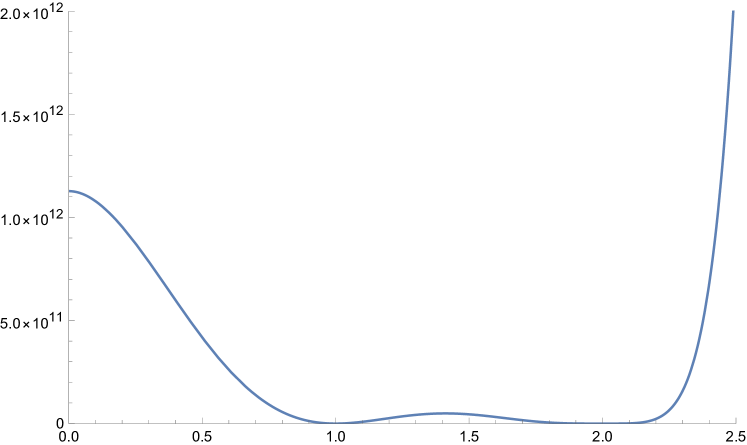
Figure 3: The function $f$ from the solution of Problem 27.

This function $f$ we gave here is not unique. Of course every multiple of $f$ also fulfills the requirements but we also made the restrictions to use all monomials except $x^{42}$. We get another polynomial when we e.g. leave out $x^{13}$ (or any other monomial except $1$) instead of $x^{42}$. Then any conic linear combination of these functions also fulfills the requirements.

We can not leave out $1$ since any linear combination has the additional zero $x=0$.

Problems of Chapter 6

prob:smoothing Proof of 8
Since $\mathcal{F}$ is a continuous T-system we can assume that

$$\det\begin{pmatrix}f_{0}&f_{1}&\dots&f_{n}\\ x_{0}&x_{1}&\dots&x_{n}\end{pmatrix}>0$$

for all $a\leq x_{0}<x_{1}<\dots<x_{n}\leq b$. Since the Gaussian kernel is ETP_k for every $k\in\mathds{N}_{0}$, see 6, we have

$$K_{\sigma}^{*}\!\begin{pmatrix}x_{1}&x_{2}&\dots&x_{n}\\ y_{1}&y_{2}&\dots&y_{n}\end{pmatrix}>0$$

for all $x_{1}<x_{2}<\dots<x_{n}$ and $y_{1}\leq y_{2}\leq\dots\leq y_{n}$ in $\mathds{R}$ as well as $\sigma>0$. Hence, in $\mathcal{W}(f_{\sigma,0},f_{\sigma,1},\dots,f_{\sigma,n})(x)=$ (53) in 7 we are integrating over a non-negative functions with respect to the Lebesgue measure $\mu=\lambda$, i.e., $\mathcal{W}(f_{\sigma,0},f_{\sigma,1},\dots,f_{\sigma,n})(x)>0$ for all $x\in[a,b]$ which proves the statement.

Problems of Chapter 7

prob:etNeighborhood The family $\mathcal{F}$ on $[a,b]$ needs for a fixed $f\geq 0$ only be an ET-system around the zeros of $f$ but otherwise the proof of 1 is employed, i.e., there we only need $\mathcal{F}$ to be a T-system.

Problems of Chapter 8

prob:posR Proof of 4 on $\mathds{R}$
By (a) there exists a function $w\in\mathcal{C}(\mathds{R},\mathds{R})$ such that $w>0$ on $\mathds{R}$ and

$$\lim_{x\to\infty}\frac{f_{n}(x)}{w(x)}=1.$$

By (b) we define

$$v_{i}(x):=\begin{cases}\frac{f_{i}(x)}{w(x)}&\text{if}\ x\in\mathds{R},\\ \delta_{i,n}&\text{if}\ x=\pm\infty\end{cases}$$

for all $i=0,1,\dots,n$. Then by (c) and 9 we have that $\{v_{i}\}_{i=0}^{n}$ is a T-system on $[0,\infty]$. With $t(x):=\tan(\pi x/2)$ we define

$$g_{i}(x):=v_{i}\circ t$$

for all $i=0,1,\dots,n$. Hence, $\mathcal{G}=\{g_{i}\}_{i=0}^{n}$ is a T-system on $[-1,1]$ by 8. We now apply 3 to $\mathcal{G}$. Set $g:=(\frac{f}{w})\circ t$.

(ii): By 3 on $[a,b]$ there exist points

$$-1=y_{0}<x_{1}<y_{1}<\dots<x_{m}<y_{m}=1$$

and unique functions $g_{*}$ and $g^{*}$ such that $g=g_{*}+g^{*}$, $g_{*},g^{*}\geq 0$ on $[-1,1]$, $x_{1},\dots,x_{m}$ are the zeros of $g_{*}$, and $y_{0},\dots,y_{m}$ are the zeros of $g^{*}$. Then $f_{*}:=(g_{*}\circ t^{-1})\cdot w$ and $f^{*}:=(g^{*}\circ t^{-1})\cdot w$ are the unique components in the decomposition $f=f_{*}+f^{*}$.

(i): Since $g^{*}(y_{0})=g^{*}(y_{m})=0$ we have that $g^{*}$ contains no $g_{2m}$ and hence the coefficient of $g_{2m}$ in $g_{*}$ is $a_{2m}$.

prob:nonnegR Proof of 5 on $\mathds{R}$
Similar to the proof of 3 on $[0,\infty)$ and hence Problem/Solution 6.

The conditions (a) – (c) are such that $\mathcal{F}$ on $[-\infty,\infty]$, i.e., including $\pm\infty$, is an ET-system.

With the same argument as in the proof of 1 we transform $\mathcal{F}$ on $[-\infty,\infty]$ into $\mathcal{G}$ on $[-1,1]$ with the $\tan$-function. Here 8 ensures that also $\mathcal{G}$ is an ET-system.

Application of 6 on $[-1,1]$ gives the desired decomposition $g=g_{*}+g^{*}$ with the observation that $x=\pm 1$ is a zero of at most multiplicity one by (a) and (b). Backwards transformation into $\mathcal{F}$ on $[-\infty,\infty]$ resp. $[-\infty,\infty)$ then gives the assertion.

Problems of Chapter 9

prob:a0 Proof of 13
10 can in general not be extended to $[0,b]$ since $\{x^{\alpha_{0}},\dots,x^{\alpha_{n}}\}$ is not an ET-system. This fails at $x=0$. But on $(0,b]$ it is an ET-system. We can therefore factor out the zeros of $f\geq 0$ at $x=0$

$$f(x)=a_{i}x^{\alpha_{i}}+a_{i+1}x^{\alpha_{i+1}}+\dots+a_{n}x^{\alpha_{n}}=x^{\alpha_{i}}\cdot(\underbrace{a_{i}+a_{i+1}x^{\alpha_{i+1}-\alpha_{i}}+\dots+a_{n}x^{\alpha_{n}-\alpha_{i}}}_{=:\tilde{f}(x)})$$

to get some $\tilde{f}$ with $\tilde{f}\geq 0$ on $[0,b]$ and $\tilde{f}(0)>0$. To $\tilde{f}$ we can then apply 10 with $a=0$.

In summary, 10 on $[0,b]$ holds if $f(0)>0$, see also 5 and 6 for the corresponding version on $[0,\infty)$.

Problems of Chapter 10

prob:nonneg0infty Proof of 5
To prove 5 we have to note that $\mathcal{F}=\{x^{\alpha_{i}}\}_{i=0}^{n}$ with $\alpha_{0}=1$ is an ET-system on $(0,\infty)$. The only difficulty is $x=0$ where $\mathcal{F}$ fails to be a ET-system.

But looking closely at the proof of 5 (see Problem/Solution 8) the ET-system property is only required in a neighborhood of the zeros of $f$ and otherwise it is the proof of 1 for T-systems. Since $f(0)>0$ we have no zero at $x=0$ where $\mathcal{F}$ fails to be a T-system. In fact, we have $f(x)>0$ for all $x\in[0,\varepsilon)$ for some $\varepsilon>0$. Hence, we can apply 3 since its proof requires for our $f$ with $f(0)>0$ only that $\mathcal{F}$ to be an ET-system on $(0,\infty)$ which is fulfilled.

prob:leadingcoeffR By expanding

$$\prod_{i=1}^{r}(x-z_{i})^{m_{i}}\cdot\left(a\cdot\prod_{i=1}^{m}(x-x_{i})^{2}+b\cdot\prod_{i=1}^{m-1}(x-y_{i})^{2}\right)$$

we see that $a\cdot x^{m_{1}+\dots+m_{r}+2m}$ is the monomial with the highest degree $m_{1}+\dots+m_{r}+2m=\deg p$ and the coefficient is $a$.

List of Symbols

Matrices

$\begin{pmatrix}f_{0}&f_{1}&\dots&f_{n}\\ x_{1}&x_{2}&\dots&x_{n}\end{pmatrix}$: 4, eq. (25)4

$\begin{pmatrix}f_{0}&\dots&f_{i-1}&f_{i}&\dots&f_{i+p}&f_{i+p+1}&\dots&f_{n}\\ x_{0}&\dots&x_{i-1}&(x_{i}&\dots&x_{i})&x_{i+p+1}&\dots&x_{n}\end{pmatrix}$: Eq. (36) 36

$\begin{pmatrix}f_{0}&f_{1}&\dots&f_{n}\\ x_{1}&x_{2}&\dots&x_{n}\end{pmatrix}^{*}$: Eq. (37) 37

$\left(\begin{array}[]{c|cccc}f_{0}&\,f_{1}&f_{2}&\dots&f_{n}\\ x&\,x_{1}&x_{2}&\dots&x_{n}\end{array}\right)$: Eq. (38) 38

Determinants

$K\!\begin{pmatrix}x_{0}&x_{1}&\dots&x_{n}\\ y_{0}&y_{1}&\dots&y_{n}\end{pmatrix}$: Eq. (48) 48

$K^{*}\!\begin{pmatrix}x_{1}&x_{2}&\dots&x_{i}\\ y_{1}&y_{2}&\dots&y_{i}\end{pmatrix}$: 3, eq. (49) 49

$\mathcal{W}(f_{0},\dots,f_{k})$: 6, eq. (40) 40

Further Mathematical Symbols

$\leq$ 1

$B_{f,d}$: Eq. (18) 18

$h_{n}\nearrow g$ 7

$\mathfrak{B}(\mathds{R}^{n})$ 6

$\mathcal{C}(\mathcal{X},\mathcal{Y})$ 2

$\mathcal{C}_{c}(\mathcal{X},\mathds{R})$ 2

$\mathrm{conv}\,A$ 4

$E_{+}$ 1

see also $(\mathrm{lin}\,\mathcal{F})_{+}$ 25

$E^{*}$ 1

$f_{+}$, $f_{-}$, $|f|$ 0.11

$\mathcal{H}(s)$: Eq. (1) 1

$\mathrm{int}\,A$ 2

$L_{\mu}$ 1.4

$\mathcal{L}^{p}(\mathcal{X},\mu)$ 6

$\varepsilon(x)$: 24, eq. (29) 24

$\varepsilon(\mathcal{X})$: 24, eq. (30) 30

$K_{\sigma}$: Eq. (50) 50

$\mathrm{lin}\,\mathcal{F}$: Eq. (24) 24

$(\mathrm{lin}\,\mathcal{F})_{+}$: 25 25

$(\mathrm{lin}\,\mathcal{F})^{e}$: 25 25

$(\mathrm{lin}\,\mathcal{F})_{+}^{e}$: 25 25

$L_{\mu}$: 1.4 1.4

$L_{s}$: 1.6 1.6

$\mathcal{M}(L)$: 1.21.2

$\mathcal{M}(\mathcal{X})_{+}$ 6

$\mathds{N}$ 1

$\mathds{N}_{0}$ 1

$\mathrm{Pos}(K)$: Eq. (12) 12

$\mathrm{Pos}(\mathds{R})$: Eq. (13) 13

$\mathrm{Pos}([0,\infty))$: Eqs. (14) and (15) 14

$\mathrm{Pos}([-1,1])$: Eq. (16) 16

$\mathrm{Pos}([a,b])$: Eq. (20) 20

$\mathcal{P}(\mathcal{X})$ 1

$\mathds{Q}$ 1

$\mathds{R}$ 1

$\mathcal{S}_{\mathcal{F}}$ 9

$\sigma(A)$ 6

$\mathds{T}$ 1

$\Xi^{m}$: Eq. (54) 54

$\mathds{Z}$ 1

Index

A

• adapted
  • cones25
  • space23
• algebra4, 27
  • $*$-27
    • Fréchet topological27
• approximation
  • best
    • polynomial117
  • Tchebycheff117 B
• Banach, S.2
• basic composition formulas73
• Basic Representation Theorem24
• Bernstein
  • polynomial32
  • Theorem32
• Bernstein, S. N.32, 44
• best approximation
  • polynomial117
• Boas’ Theorem38
• Boas, R. P.35, 38,  108
• Borel
  • measure4
  • $\sigma$-algebra4
• Brickman, L.33 C
• Carathéodory
  • Theorem3
• Carroll, L.57
• compact
  • locally
    • Hausdorff space2
  • set2
• cone3
  • adapted25
  • negative1
  • positive1
    • linear functional21
• Conic Extension Theorem26
• continuous2
• convex3
• cubature formula
  • Gaussian37
• Curtis–Mairhuber–Sieklucki Theorem47 D
• Daniell’s Representation Theorem6
• Daniell’s Signed Representation Theorem9
• Daniell, P. J.6
• decomposition
  • Riesz property12
• determinant
  • representation as a49,  68
  • Vandermonde44, 48
  • Wronskian60
• determinate
  • moment functional19
• Dirac, P. A. M.105
• dominate23
  • cone25
• dual2 E
• ECT-system60
• Einstein, A.1
• ET-system57
• ETP_k72
• Euripides71
• extended
  • totally
    • positive72 F
• Fil’štinskiǐ, V. A.34
• Fixed Point Theorem of Brouwer79
• Fréchet space27
• function
  • measurable4
  • $\mu$-integrable4
• functional
  • $K$-moment18
  • linear27
    • cone positive21
    • non-negative27
  • moment17
  • Riesz18
  • sublinear2
  • superlinear2
• Fundamental Theorem of Algebra110 G
• Gauß, C. F.37
• Gaussian kernel72 H
• Haar, A.118
• Hahn, H.2
• Hahn–Banach Theorem2
• Hamburger moment problemsee Theorem, Hamburger31
• Hamburger’s Theorem30
• Hamburger, H. L.30, 39
• Hankel matrix3
  • of a sequence3, 18
• Hardy, G. H.77
• Hausdorff
  • moment problem
    • sparse102
  • space2
  • truncated moment problem
    • sparse101
• Hausdorff moment problemsee Theorem, Hausdorff32
• Hausdorff’s Theorem30
• Hausdorff, F.30, 35,  101
• Haviland’s Theorem31
• Haviland, E. K.31
• Haviland–Hildebrandt–Schoenberg–Wintner Theorem34
• Haviland–Wintner Theorem34
• Helly, E.2
• Herglotz
  • moment problem31
• Hilbert, D.32
• Hildebrandt, T. H.34
• hull
  • convex3 I
• identity
  • Sylvester62
• indeterminacy
  • Stieltjes example19
• indeterminate
  • moment
    • functional19
• index52
  • of a set52
• interior
  • of a set2
• Interlacing Theoremsee Snake Theorem83 J
• Jackson, D.121 K
• $K$-moment functional18
• Kakutani, S.11
• Karlin
  • Nichtnegativstellensatz
    • on $[0,\infty)$91
    • on $[a,b]$86
    • on $\mathds{R}$92
  • Positivstellensatz
    • on $[0,\infty)$89
    • on $[a,b]$82
    • on $\mathds{R}$92
  • Theorem
    • for $f>0$ on $[a,b]$77
    • for $f\geq 0$ on $[a,b]$84
• Karlin, S.vii
• kernel71
  • Gaussian72
• Krein, M. G.33, 83 L
• lattice
  • of functions5
  • space5
• Leibniz, G. W.97
• Lemma
  • Markov82
• Lewin, K.43
• locally compact2
• Lukács Theoremsee Lukács–Markov Theorem33
• Lukács, F.33
• Lukács–Markov Theorem33,  99 M
• majorized21
• Markov Lemma82
• Markov’s Theoremsee Lukács–Markov Theorem33
• Markov, A. A.11, 33
• Markov–Lukács Theoremsee Lukács–Markov Theorem34
• measurable
  • function4
  • space4
• measure4
  • Borel4
  • Carathéodory outer4
  • outer4
  • Radon4
  • regular5
  • representing17
  • space4
• Milton, J.113
• minorized21
• moment
  • $f$-moment of $\mu$17
  • functional17
    • determinate19
    • generated by $\mu$18
    • indeterminate19
    • truncated19
  • problem
    • Hamburgersee Theorem, Hamburger30
    • Hausdorffsee Theorem, Hausdorff30
    • Herglotz31
    • Stieltjessee Theorem, Stieltjes29
    • Švencosee Theorem, Švenco34
    • trigonometric31
  • sequence18
• $\mu$-integrable4
• $\mu$-measurable4 N
• negative cone1
• neighborhood2
• Nichtnegativstellensatz
  • Karlin
    • on $[0,\infty)$91
    • on $[a,b]$86
    • on $\mathds{R}$92
• Nudel’man, A. A.33, 83 O
• optimization
  • over linear functionals121
• order
  • partial1
  • total1
  • vector space1
• orthogonal
  • polynomial121 P
• Pólya, G.32, 39,  89
• partial order1
• polynomial44
  • Bernstein32
  • best approximation117
  • orthogonal121
  • Schur68
• Pope, A.17
• positive
  • totally71
    • extended72
    • strictly71
• positive cone1
• Positivstellensatz
  • Karlin
    • on $[0,\infty)$89
    • on $[a,b]$82
    • on $\mathds{R}$92 R
• Radau, M. R.33
• Radon
  • measure4
• reduced
  • system61, 63
• regular
  • measure5
• representation
  • as a determinant49, 68
  • Theorem
    • Basic24
    • Daniell6
    • Daniell, signed9
    • Riesz12
    • Riesz, signed11
    • Riesz–Markov–Kakutani11
• representing
  • measure17
• Richter’s Theorem36
• Richter, H.35
• Richter–Rogosinski–Rosenbloom Theorem38
• Riesz
  • decomposition property12
• Riesz functional18
• Riesz’ Representation Theorem12
  • Signed11
• Riesz, F.11
• Riesz, M.31
• Riesz–Markov–Kakutani Representation Theorem11
• Rogosinski, W. W.38
• Rosenbloom, P. C.37 S
• Santayana, G.29
• Schmüdgen, K.39
• Schoenberg, I. J.34
• Schur polynomial68
• sequence
  • moment18
• Shakespeare, W.117
• Sherman, T.39
• $\sigma$-algebra4
  • Borel4
• Snake Theorem83
• space
  • adapted23
  • Hausdorff2
    • locally compact2
  • lattice5
  • measurable4
  • measure4
  • topological2
• sparse
  • algebraic Nichtnegativstellensatz
    • on $[0,\infty)$109
    • on $[0,b]$104
    • on $[a,b]$103
    • on $\mathds{R}$110
  • algebraic Positivstellensatz
    • on $[0,\infty)$105
    • on $[a,b]$97
    • on $\mathds{R}$110
  • Hausdorff moment problem101, 102
    • truncated101
  • Stieltjes moment problem108
• Stieltjes
  • example
    • indeterminacy19
• Stieltjes moment problemsee Theorem, Stieltjes32
• Stieltjes’ Theorem29
• Stieltjes, T. J.19, 29
• Stochel, J.39
• Stone–Weierstrass Theorem3
• STP_k71
• Strassen’s Theorem22
• strictly
  • totally
    • positive71
• sublinear
  • functional2
• suits6
• superlinear
  • functional2
• Švenco’s Theorem34
• Švenco, K. I.34
• Sylvester’s identity62
• system
  • ECT-60
  • ET-57
  • reduced61, 63
  • T-44
  • Tchebycheffsee T-44
• Szegö, G.32 T
• T-system44
  • continuous45
  • extended57
    • complete60
  • periodic45
• Tchakaloff, M. V.37
• Tchebycheff approximation117
• Tchebycheff systemsee T-system44
• Tchebycheff, P. L.43
• Theorem
  • Algebra
    • Fundamental110
  • Basic Representation24
  • Bernstein32
  • Boas38
  • Brouwer Fixed Point79
  • Carathéodory3
  • Conic Extension26
  • Curtis–Mairhuber–Sieklucki47
  • Daniell’s Representation6
    • Signed9
  • Hahn–Banach2
  • Hamburger30
  • Hausdorff30
    • sparse101
  • Haviland31
  • Haviland–Hildebrandt–Schoenberg–Wintner34
  • Haviland–Wintner34
  • Interlacingsee Snake83
  • Karlin
    • for $f>0$ on $[a,b]$77
    • for $f\geq 0$ on $[a,b]$84
    • Nichtnegativstellensatz on $[0,\infty)$91
    • Nichtnegativstellensatz on $[a,b]$86
    • Nichtnegativstellensatz on $\mathds{R}$92
    • Positivstellensatz on $[0,\infty)$89
    • Positivstellensatz on $[a,b]$82
    • Positivstellensatz on $\mathds{R}$92
  • Lukácssee Lukács–Markov33
  • Lukács–Markov33, 99
  • Markovsee Lukács–Markov33
  • Markov–Lukácssee Lukács–Markov34
  • Müntz–Szász102
  • Richter36
  • Richter–Rogosinski–Rosenbloom38
  • Riesz’ Representation12
    • Signed11
  • Riesz–Markov–Kakutani Representation11
  • Rogosinski38
  • Rosenbloom37
  • Snake83
  • Stieltjes29
  • Stone–Weierstrass3
  • Strassen22
  • Švenco34
  • Tchakaloff37
  • Wald37
• topology2
• total order1
• totally
  • positive71
• TP_k71
• trigonometric
  • moment problem31
• truncated
  • moment functional19 U
• unit element27 V
• Vandermonde
  • determinant44, 48
• vector space
  • ordered1 W
• Wald, A.37
• Wiener, N.21
• Wintner, A.31
• Wronskian60
• Wronskian determiantsee Wronskian60 Z
• zero
  • multiplicity57
  • nodal50
  • non-nodal50

References

- AAM (96) A. G. Akritas, E. K. Akritas, and G. I. Malaschonok, Various proofs of Sylvester’s (determinant) identity, Math. Comput. Simulat. 42 (1996), 585–593.
- Ach (56) N. I. Achieser, Theory of Approximation, Frederick Ungar, New York, 1956.
- AK (62) N. I. Ahiezer and M. Kreĭn, Some Questions in the Theory of Moments, American Mathematical Society, Providence, Rhode Island, 1962.
- (4) S. Banach, Sur les fonctionnelles linéaires I, Stud. Math. 1 (1929), 211–216.
- (5) , Sur les fonctionnelles linéaires II, Stud. Math. 1 (1929), 223–239.
- Ber (12) S. N. Bernstein, Démonstration du théorème de Weierstrass fondée sur le calcul des probabilités, Comm. Kharkiv Math. Soc. 13 (1912), 1–2.
- Ber (15) , Sur la représentation des polynômes positifs, Comm. Kharkiv Math. Soc., 2nd series 14 (1915), 227–228.
- Ber (26) , Leçons sur les Propriétés extrémales et la Meilleure Approximation des Fonctions Analytique d’une Variable rèelle, Gauthier–Villars, Paris, 1926.
- Ber (37) , Extremal properties of polynomials and the best approximation of continuous functions of one real variable, vol. 1, ONTI, Leningrad-Moscow, 1937.
- (10) R. P. Boas, On a generalization of the Stieltjes moment problem, Trans. Amer. Math. Soc. 46 (1939), 142–150.
- (11) , The Stieltjes moment problem for functions of bounded variation, Bull. Amer. Math. Soc. 45 (1939), 399–404.
- Bog (07) V. I. Bogachev, Measure Theory, Springer-Verlag, Berlin, 2007.
- Bri (59) L. Brickman, A new generalization of a problem of F. Lukács, Compos. Math. 14 (1959), 195–227.
- Bro (11) L. E. J. Brouwer, Über Abbildungen von Mannigfaltigkeiten, Math. Ann. 71 (1911), 97–115.
- Car (11) C. Carathéodory, Über den Variabilitätsbereich der Fourier’schen Konstanten von positiven harmonischen Funktionen, Rend. Circ. Mat. Palermo 32 (1911), 193–217.
- CdD (22) R. Curto and P. J. di Dio, Time-dependent moments from the heat equation and a transport equation, Int. Math. Res. Notices (2022), https://doi.org/10.1093/imrn/rnac244.
- Cho (69) G. Choquet, Lectures on Analysis, W. A. Benjamin, Inc., New York, Amsterdam, 1969, 3 volumes.
- Cur (59) P. C. Curtis, Jr., -parameter families and best approximation, Pacific J. Math. 9 (1959), 1013–1027.
- Dan (18) P. J. Daniell, A General Form of Integral, Ann. Math. 19 (1918), 279–294.
- Dan (20) , Further Properties of the General Integral, Ann. Math. 21 (1920), 203–220.
- dD (23) P. J. di Dio, The Early History of Moment Problems and Non-Negative Polynomials with Gaps: Sparse Moment Problems, Sparse Positivstellensätze, and Sparse Nichtnegativstellensätze from a T-System Point of View, unpublished manuscript, arXiv:2309.03864.
- dDS (22) P. J. di Dio and K. Schmüdgen, The multidimensional truncated moment problem: The moment cone, J. Math. Anal. Appl. 511 (2022), 126066, 38 pages.
- Dir (58) P. A. M. Dirac, The Principles of Quantum Mechanics, 4th ed., Oxford University Press, Oxford, 1958, with revisions in 1967.
- Edw (78) D. A. Edwards, On the existence of probablity measures with given marginales, Ann. Inst. Fourier, Grenoble 28 (1978), no. 4, 53–78.
- Ein (35) A. Einstein, The Late Emmy Noether. Professor Einstein Writes in Appreciation of a Fellow-Mathematician., The New York Times (May 4, 1935), 12.
- Eur (13) Euripides, Euripides II: Andromache, Hecuba, the Suppliant Women, Electra, 3rd ed., The University of Chicago Press, Chicago, London, 2013.
- Fed (69) H. Federer, Geometric Measure Theory, Springer-Verlag, Berlin, 1969.
- Fil (64) V. A. Fil’štinkiǐ, The power moment problem on the entire axis with a finite number of empty intervals in the spectrum, Zap. Meh.-Mat. Fak. i Harkow. Mat. Obšč 40 (1964), 186–200, in Russian.
- FP (01) C. F. Floudas and P. M. Pardalos (eds.), Encyclopedia of Optimization, vol. 1, Kluwer Academic Publishers, Dordrecht, 2001.
- Gau (15) C. F. Gauß, Methodus nova integralium valores per approximationem inveniendi, Comm. Soc. Sci. Göttingen Math. 3 (1815), 29–76.
- GK (02) V. Gantmacher and M. Krein, Oscillation matrices and kernels and small vibrations of mechanical systems, American Mathematical Society, Providence, RI, 2002, originally published in Russian, Moskow, 1950.
- GM (96) M. Gasca and C. A. Micchelli (eds.), Total Positivity and Its Applications, Mathematics and Its Applications, no. 359, Springer Science+Business Media, Dordrecht, 1996.
- Gon (00) V. L. Goncharov, The Theory of Best Approximation of Functions, J. Approx. Theo. 106 (2000), 2–57.
- Haa (18) A. Haar, Die Minkowskische Geometrie und die Annäherung an stetige Funktionen, Math. Ann. 78 (1918), 294–311.
- Hah (27) H. Hahn, Über lineare Gleichungssysteme in linearen Räumen, J. reine angew. Math. 157 (1927), 214–229.
- Ham (20) H. L. Hamburger, Über eine Erweiterung des Stieltjesschen Momentenproblems, Math. Ann. 81 (1920), 235–319.
- Har (69) G. H. Hardy, A Mathematician’s Apology, Cambridge University Press, London, 1969, reprint of the first edition from 1940, with a forword of C. P. Snow.
- (38) F. Hausdorff, Summationsmethoden und Momentenfolgen I, Math. Z. 9 (1921), 74–109.
- (39) , Summationsmethoden und Momentenfolgen II, Math. Z. 9 (1921), 280–299.
- Hav (35) E. K. Haviland, On the momentum problem for distribution functions in more than one dimension, Amer. J. Math. 57 (1935), 562–572.
- Hav (36) , On the momentum problem for distribution functions in more than one dimension II, Amer. J. Math. 58 (1936), 164–168.
- Hel (12) E. Helly, Über lineare Funktionaloperatoren, Sitzungsber. Akad. Wiss. Wien 121 (1912), 265–297.
- Hil (88) D. Hilbert, Über die Darstellung definiter Formen als Summe von Formenquadraten, Math. Ann. 32 (1888), 342–350.
- HS (33) T. H. Hildebrandt and I. J. Schoenberg, On Linear Functional Operations and the Moment Problem for a Finite Interval in One or Several Dimensions, Ann. Math. 34 (1933), 317–328.
- Jac (24) D. Jackson, A general class of problems in approximation, Am. J. Math. XLVI (1924), 215–234.
- Kak (41) S. Kakutani, Concrete representation of abstract (M)-spaces (A characterization of the space of continuous functions), Ann. Math. Series 2 42 (1941), 994–1024.
- Kar (63) S. Karlin, Representation Theorems for Positive Functions, J. Math. Mech. 12 (1963), 599–618.
- Kar (68) , Total Positivity, vol. 1, Stanford University Press, Stanford, California, 1968.
- Kem (68) J. H. B. Kemperman, The General Moment Problem, a Geometric Approach, Ann. Math. Stat. 39 (1968), 93–122.
- KN (77) M. G. Kreĭn and A. A. Nudel’man, The Markow Moment Problem and Extremal Problems, American Mathematical Society, Providence, Rhode Island, 1977, translation of the Russian original from 1973.
- Kre (51) M. G. Kreĭn, The ideas of P. L. Čebyšev and A. A. Markov in the theory of limiting values of integrals and their further development, Uspehi Mat. Nauk 6 (1951), no. 4 (44), 3–120, English transl.: Amer. Math. Soc. Transl. (2) 12 (1959), 1–121.
- KS (53) S. Karlin and L. S. Shapley, Geometry of moment spaces, Mem. Amer. Math. Soc. 12 (1953).
- KS (66) S. Karlin and W. J. Studden, Tchebycheff Systems: With Applications in Analysis and Statistics, John Wiley & Sons, Interscience Publishers, New York, NY, 1966.
- Lau (09) M. Laurent, Sums of squares, moment matrices and optimization over polynomials, Emerging application of algebraic geometry, IMA Vol. Math. Appl., vol. 149, Springer, New York, 2009, pp. 157–270.
- Lei (89) G. W. Leibniz, Philosophical Essays, Hackett Publishing Company, Inc., Indianapolis, Indiana, 1989, p. 1, letter to Foucher in 1675, in French.
- Lew (43) K. Lewin, Psychology and the Process of Group Living, J. Soc. Psych. S.P.S.S.I. Bull. 17 (1943), 113–131.
- Lin (99) T. Lindvall, On Strassen’s Theorem on stochastic Domination, Elect. Comm. in Probab. 4 (1999), 51–59.
- Lor (86) G. G. Lorentz, Bernstein Polynomials, AMS Chelsea Publishing, Providence, Rhode Island, 1986.
- Luk (18) F. Lukács, Verschärfung des ersten Mittelwertsatzes der Integralrechnung für rationale Polynome, Math. Z. 2 (1918), 295–305.
- Mac (95) I. G. Macdonald, Symmetric Functions and Hall Polynomials, 2nd ed., Oxford Science Publications, Oxford, 1995.
- Mai (56) J. C. Mairhuber, On Haar’s theorem concering Chebyshev approximation problems having unique solutions, Proc. Amer. Math. Soc. 7 (1956), 609–615.
- Mar (84) A. A. Markov, On certain applications of algebraic continued fractions, Thesis (in Russian), St. Petersburg, 1884, 131 pp.
- Mar (95) , Deux démonstrations de la convergence de certaines fractions continues, Acta Math. 19 (1895), 93–104.
- Mar (06) , Lectures on functions deviating least from zero, Mineographed Notes, St. Petersburg, 1906, in Russian; reprinted in A. A. Markov, Selected papers on continued fractions and the theory of functions deviating least from zero, OGIZ, Moscow, 1948, p. 244–291.
- Mar (38) A. Markov, On mean values and exterior densities, Rec. Math. Moscou. N.S. 4 (1938), 165–190.
- Mar (08) M. Marshall, Positive Polynomials and Sums of Squares, Mathematical Surveys and Monographs, no. 146, American Mathematical Society, Rhode Island, 2008.
- Mün (14) C. H. Müntz, Mathematische Abhandlungen Hermann Amandus Schwarz zu seinem fünfzigjährigen Doktorjubiläum am 6. August 1914 gewidmet von Freunden und Schülern., ch. Über den Approximationssatz von Weierstrass, pp. 303–312, Springer, Berlin, 1914.
- NW (72) S.-B. Ng and S. Warner, Continuity of positive and multiplicative functionals, Duke Math. J. 39 (1972), 281–284.
- Phe (01) R. R. Phelps, Lectures on Choquet’s Theorem, Springer-Verlag, Berlin, Heidelberg, 2001.
- Pie (07) A. Pietsch, History of Banach Spaces and Linear Operators, Birkhäuser, Boston, 2007.
- Pól (38) G. Pólya, Sur l’indétermination d’un théoreme voisin du probléme des moments, C. R. Acad. Sci. Paris 207 (1938), 708–711.
- Pól (45) , How To Solve It. A New Aspect of Mathematical Method, Princeton University Press, Princeton, NJ, 1945, reprinted 2022 in Pinguin Books.
- PS (64) G. Pólya and G. Szegö, Aufgaben und Lehrsätze aus der Analysis, 3rd ed., vol. 2, Springer-Verlag, Berlin, 1964.
- PS (70) , Aufgaben und Lehrsätze aus der Analysis, 4th ed., vol. 1, Springer-Verlag, Berlin, 1970.
- Rad (80) R. Radau, Étude sur les formules d’approximation qui servant à calculer la valeur numérique d’une intégrale définie, J. Math. Pures Appl., 3 série 6 (1880), 283–336.
- Ric (57) H. Richter, Parameterfreie Abschätzung und Realisierung von Erwartungswerten, Bl. Deutsch. Ges. Versicherungsmath. 3 (1957), 147–161.
- Rie (09) F. Riesz, Sur les opérations fonctionnelles linéaires, C. R. Acad. Sci. Paris 144 (1909), 1409–1411.
- Roc (72) R. T. Rockafellar, Convex Analysis, Princeton University Press, Princeton, New Jersey, 1972.
- Rog (58) W. W. Rogosinski, Moments of non-negative mass, Proc. R. Soc. Lond. A 245 (1958), 1–27.
- Ros (52) P. C. Rosenbloom, Quelques classes de problème extrémaux. II, Bull. Soc. Math. France 80 (1952), 183–215.
- San (05) G. Santayana, Reason in Common Sense, The Life of Reason, vol. 1, London Constable, London, 1905.
- Sch (53) I. J. Schoenberg, On smoothing operations and their generating functions, Bull. Amer. Math. Soc. 59 (1953), 199–230.
- Sch (78) K. Schmüdgen, Uniform Topologies on Enveloping Algebras, J. Funct. Anal. 39 (1978), 57–66.
- Sch (90) , Unbounded Operator Algebras and Representation Theory, Birkhäuser, Basel, Boston, Berlin, 1990.
- Sch (91) , The -moment problem for closed semi-algebraic sets, Math. Ann. 289 (1991), 203–206.
- Sch (14) R. Schneider, Convex Bodies: The Brunn–Minkowski Theory, Cambridge University Press, Cambridge, 2014.
- Sch (17) K. Schmüdgen, The Moment Problem, Springer, New York, 2017.
- She (64) T. Sherman, A Moment Problem on , Rend. Circ. Mat. Palermo 13 (1964), 273–278.
- Sie (58) K. Sieklucki, Topological properties of sets admitting the Tschebycheff systems, Bull. Acad. Polon. Sci. Sér. Sci. Math. Astr. Phys. 6 (1958), 603–606.
- Ska (93) J. Skala, The Existence of probability Measures with given Marginals, Ann. Prob. 21 (1993), 136–142.
- ST (43) J. A. Shohat and J. D. Tamarkin, The Problem of Moments, Amer. Math. Soc., Providence, R.I., 1943.
- Sti (94) T. J. Stieltjes, Recherches sur les fractions continues, Ann. Fac. Sci. Toulouse 8 (1894), no. 4, J1–J122.
- Sto (37) M. H. Stone, Applications of the theory of Boolean rings to general topology, Trans. Amer. Math. Soc. 41 (1937), 375–481.
- Sto (01) J. Stochel, Solving the truncated moment problem solves the moment problem, Glasgow J. Math. 43 (2001), 335–341.
- Str (65) V. Strassen, The existence of probability measures with given marginales, Ann. Math. Stat. 36 (1965), 423–439.
- Šve (39) K. I. Švenco, On Hamburger’s moment problem with supplementary requirement that masses are absent on a given interval, Commun. Soc. Math. Kharkov 16 (1939), 121–128, in Russian.
- SW (99) H. H. Schaefer and M. P. Wolff, Topological Vector Spaces, Graduate Texts in Mathematics, no. 3, Springer Science+Business Media, New York, 1999.
- Syl (51) J. J. Sylvester, On the relation between the minor determinants of linearly equivalent quadratic functions, Phil. Mag. 1 (1851), 295–305.
- Szá (16) O. Szász, Über die Approximation stetiger Funktionen durch lineare Aggregate von Potenzen, Math. Ann. 77 (1916), 482–496.
- Tch (74) P. L. Tchebycheff, Sur les values limites des intégrales, J. Math. Pures Appl. (2) 19 (1874), 157–160.
- Tch (57) M. V. Tchakaloff, Formules de cubatures méchaniques a coefficients non négatifs, Bull. Sci. Math. 81 (1957), 123–134.
- Toe (11) O. Toeplitz, Über allgemeine lineare Mittelbildung, Prace Mat.-Fiz. 22 (1911), 113–119.
- Trè (67) F. Trèves, Topological Vector Spaces, Distributions and Kernels, Academic Press, New York, 1967.
- Ury (25) P. Urysohn, Über die Mächtigkeit der zusammenhängenden Mengen, Math. Ann. 94 (1925), 262–295.
- Wal (39) A. Wald, Limits of distribution function determined by absolute moment and inequalities satisfied by absolute moments, Trans. Amer. Math. Soc. 46(2) (1939), 280–306.
- Wei (85) K. Weierstrass, Über die analytische Darstellbarkeit sogenannter willkürlicher Functionen reeller Argumente, Sitzungsber. Königl. Preuss. Akad. Wiss. (9. Juli 1885), 633–639.
- Wer (07) D. Werner, Funktionalanalysis, Springer-Verlag, Berlin, 2007.
- Wie (88) N. Wiener, The Human Use of Human Beings: Cybernetics and Society, Da Capo Press, Cambridge, Massachusetts, 1988.
- Xia (59) D. Xia, Positive functional on algebras, Dokl. Akad. Nauk SSSR 124 (1959), 1223–1225, Izv. Akad. Nauk, SSS4, Ser. Mat. 23 (1959), 509–528; in Russian.
- Yos (68) K. Yosida, Functional Analysis, 2nd ed., Springer-Verlag, Berlin, 1968.
- Zei (86) E. Zeidler, Nonlinear Functional Analysis and its Applications I: Fixed-Point Theorems, Springer, New York, 1986.