Improve Generalization Ability of Deep Wide Residual Network with A Suitable Scaling Factor

Abstract

Deep Residual Neural Networks (ResNets) have demonstrated remarkable success across a wide range of real-world applications. In this paper, we identify a suitable scaling factor (denoted by $\alpha$) on the residual branch of deep wide ResNets to achieve good generalization ability. We show that if $\alpha$ is a constant, the class of functions induced by Residual Neural Tangent Kernel (RNTK) is asymptotically not learnable, as the depth goes to infinity. We also highlight a surprising phenomenon: even if we allow $\alpha$ to decrease with increasing depth $L$, the degeneration phenomenon may still occur. However, when $\alpha$ decreases rapidly with $L$, the kernel regression with deep RNTK with early stopping can achieve the minimax rate provided that the target regression function falls in the reproducing kernel Hilbert space associated with the infinite-depth RNTK. Our simulation studies on synthetic data and real classification tasks such as MNIST, CIFAR10 and CIFAR100 support our theoretical criteria for choosing $\alpha$.

1 Introduction

Recently, state-of-the-art deep residual neural networks (ResNets) [12] have become popular in many real-world domains, such as image classification [33, 12], face recognition [34], handwritten digit string recognition [36], and others [28, 14, 26, 30, 10]. ResNets are equipped with residual connections, fitted by black-box optimization, and often designed with such complexity that leads to interpolation. It is composed of multiple blocks, with each block containing two or three layers. The input of each block is added to the output of the block and the sum becomes the input of the next block. This residual structure of ResNet allows it to be designed much deeper than feedforward neural networks and significantly improves the generalization performance. For example, [12] proposed ResNet-152, which consists of 152 layers and can achieve a top-1 accuracy of 80.62% on the ImageNet dataset. ResNet-1001 proposed in [13] can achieve a 95.08% accuracy on the CIFAR-10 dataset.

Although ResNets have demonstrated superior performance over classical feedforward neural networks (FNNs) in many applications, the reasons behind this have not been clearly elucidated. Several insightful studies have been conducted to explore this topic empirically. [32] claimed that ResNet behaves like a collection of relatively shallow neural networks, thus alleviating the problem of vanishing gradients. [3] further investigated the issue of shattered gradients and found that gradients in networks with residual connections decay sublinearly with depth, while those in FNNs decay exponentially, leading to corresponding gradient descent that looks like white noise. As a result, gradients in ResNets are far less anti-shattering than FNNs. [21] visualized the surfaces of different neural networks and found that networks with skip connections often have smoother loss surfaces, making them less likely to be trapped in local minima and easier to optimize.

Another line of research focuses on the theoretical properties of finite-width ResNet, including convergence properties and generalization ability. [11] proved that every critical point of a linear residual network is a global minimum. [24] demonstrated that a two-layer ResNet trained using stochastic gradient descent (SGD) converges to a unique global minimum in polynomial time. [1] claimed that gradient descent (GD) and SGD can find the global minimum in polynomial time for a general $L$-block ResNet. [38] study the stability and convergence of training with respect to different choice of $\alpha$. [22, 9] derived generalization bounds for $L$-block ResNet based on the GD algorithm.

The research conducted by [17] presents a valuable theoretical framework for investigating overparameterized feed forward neural networks (FNNs). They demonstrated that during the training process of FNNs with sufficient width, weight matrices remain close to their initial values. Moreover, the training of FNNs with infinite width can be interpreted as a kernel regression using a fixed kernel known as the neural tangent kernel (NTK) in a reproducing kernel Hilbert space (RKHS). Notably, the NTK is solely dependent on the initialized weight matrices. Expanding upon the concept of the NTK, recent works by [18, 23] have provided theoretical evidence that the generalization error of wide fully-connected neural networks can be approximated through kernel regression using the NTK. These findings suggest that it is feasible to study the generalization ability of neural networks by analyzing the generalization ability of kernel regression.

Several studies have investigated the NTK for residual networks. In [16], the Residual Neural Network Kernel (RNK) was introduced, and it was demonstrated that the RNK at initialization converges to the NTK for residual networks. The study also showed that infinitely deep NTK of feedforward neural networks (FCNTK) degenerates, leading to a constant output for any input, which illustrates the advantage of ResNet over FNN. In [31], the stability of RNK was shown, and the convergence of RNK to the NTK during training with gradient descent was demonstrated. However, the commonly used activation function, ReLU, does not satisfy the assumptions in [31]. The authors also showed that RNTK induced a smoother function space than FCNTK. In [4], it was shown that for inputs distributed uniformly on the hypersphere $\mathbb{S}^{d-1}$, the eigenvalues of the NTK for residual networks decay polynomially with frequency $k$ with $k^{-d}$, and the set of functions in ResNet’s RKHS is identical to that of FC-NTK. In [19], it was shown that the properties of FC-NTK in [18, 23] also hold for RNTK.

From any perspective, the unique design of ResNet blocks is believed to be the key factor in the improved performance compared to FNNs. The scaling factor on the residual branch of ResNet (denoted by $\alpha$), which controls the balance between the input and output, is crucial in achieving the impressive performance of ResNets. Different literature suggests different settings of $\alpha$. For example, [37] suggest $\alpha$ to decay with depth. [16, 8] suggest setting this parameter to be $\alpha=L^{-\gamma}$ with a constant $\gamma$ satisfying $\frac{1}{2}\leq\gamma\leq 1$. In contrast, [12] set $\alpha$ to be $1$. [4] show that the choice of $\alpha$ has a significant effect on the shape of ResNTK for deep architecture, ResNTK can either become spiky with depth, as with FC-NTK, or maintain a stable shape. However, there are scarce studies of the influence of the scaling factor on the residual branch on the generalization ability of ResNet.

1.1 Major contributions

In this article, we address the limitations in the theory of the generalization ability of ResNet. Specifically, we explore the influence of the scaling factor $\alpha$ on the generalization ability of ResNet and aim to identify a good choice of $\alpha$ for better generalization performance. To achieve this, we utilize the NTK tool and analyze the large $L$ limit of RNTK, since ResNets are typically designed to be very deep.

Firstly, we establish some important spectral properties of the RNTK and demonstrate that the generalization error of ResNet can be well approximated by kernel regression using the RNTK. This approximation holds for any value of $L\geq 1$ and $\alpha=C\cdot L^{-\gamma}$, where $\gamma$ ranges from $0$ to $1$, and $C>0$ is an arbitrary constant. Then we show that when $\alpha$ is a constant, the corresponding RNTK with infinite depth degenerates to a constant kernel, resulting in poor generalization performance. We also indicate a surprising phenomenon that even if we allow $\alpha$ to decrease with increasing depth, the degeneration phenomenon may still exist. However, when $\alpha$ decreases sufficiently fast with depth, i.e., $\alpha=L^{-\gamma}$ where $\gamma\in(1/2,1]$, the corresponding kernel converges to a one-hidden-layer FCNTK. Further, kernel regression with the one-hidden-layer FCNTK optimized by gradient descent can achieve the minimax rate with early stopping. These theoretical results suggest that $\alpha$ should decrease with increasing depth quickly. Our simulation studies, using both artificial data and CIFAR10/MNIST datasets, on RNTK and finite width convolutional residual network, support our criteria for choosing $\alpha$.

To the best of our knowledge, this is the first paper to fully characterize the generalization ability of ResNet with various choices of $\alpha$. It provides an easy-to-implement guideline for choosing $\alpha$ in practice to achieve better generalization ability and helps to demystify the success of ResNet to a large extent.

The rest of this paper is organized as follows. In Section 2.1, we give a brief review of some important properties of RNTK. Behaviour of infinite-depth RNTK in different choice of $\alpha$ are shown in Section 3. Section 4 contains our experiment studies including the comparison of different choices of $\alpha$. Lastly, Section 5 concludes discussion and future directions of this paper.

Notations and model settings

Let $f_{*}$ be a continuous function defined on a compact subset $\mathcal{X}\subseteq\mathbb{S}^{d-1}$, the $d-1$ dimensional sphere satisfying $\mathbb{S}^{d-1}:=\{\boldsymbol{x}\in\mathbb{R}^{d}:\|\boldsymbol{x}\|=1\}$. Let $\mu_{\mathcal{X}}$ be a uniform measure supported on $\mathcal{X}$. Suppose that we have observed $n$ i.i.d. samples $\mathcal{D}_{n}=\{(\boldsymbol{x}_{i},y_{i}),i\in[n]\}$ sampling from the model:

$$y_{i}=f_{*}(\boldsymbol{x}_{i})+\varepsilon_{i},\quad i=1,\dots,n,$$

where $\boldsymbol{x}_{i}$’s are sampled from $\mu_{\mathcal{X}}$, $\varepsilon_{i}\sim\mathcal{N}(0,\sigma^{2})$ (the centered normal distribution with variance $\sigma^{2}$) for some fixed $\sigma>0$ and $[n]$ denotes the index set $\{1,2,...,n\}$. We collect $n$ i.i.d. samples into matrix $\boldsymbol{X}:=(\boldsymbol{x}_{1},\dots,\boldsymbol{x}_{n})^{\top}\in\mathbb{R}^{n\times d}$ and vector $\boldsymbol{y}:=(y_{1},\dots,y_{n})^{\top}\in\mathbb{R}^{n}$. We are interested in finding $\hat{f}_{n}$ based on these $n$ samples, which can minimize the excess risk, i.e., the difference between $\mathcal{L}(\hat{f}_{n})=\boldsymbol{E}_{(\boldsymbol{x},y)}\left[(\hat{f}_{n}(\boldsymbol{x})-y)^{2}\right]$ and $\mathcal{L}(f_{*})=\boldsymbol{E}_{(\boldsymbol{x},y)}\left[(f_{*}(\boldsymbol{x})-y)^{2}\right]$. One can easily verify the following formula about the excess risk:

$$\mathcal{E}(\hat{f}_{n})=\mathcal{L}(\hat{f}_{n})-\mathcal{L}(f_{*})=\int_{\mathcal{X}}\left(\hat{f}_{n}(\boldsymbol{x})-f_{*}(\boldsymbol{x})\right)^{2}\mathrm{d}\mu_{\mathcal{X}}(\boldsymbol{x}).$$

It is clear that the excess risk is an equivalent evaluation of the generalization performance of $\hat{f}_{n}$.

For two sequences $a_{n}$ and $b_{n}$, we write $a_{n}={O}(b_{n})$ (resp. $a_{n}=\Omega(b_{n})$) when there exists a positive constant $C$ such that $a_{n}\leqslant Cb_{n}$ (resp. $a_{n}\geqslant C^{\prime}b_{n}$). We write $a_{n}=o(b_{n})$ if $\lim\limits_{n\to\infty}a_{n}/b_{n}=0$. We will use $\text{poly}(x,y,\dots)$ to represent a polynomial of $x,y,\dots$ whose coefficients are absolute constants.

2 Properties of RNTK

2.1 Review of RNTK

Network Architecture and Initialization

In the following, we work with following definition of ResNet, which has been implemented in [16, 4, 31, 19] as follows:

$$f(\boldsymbol{x},\boldsymbol{\theta}) =\boldsymbol{v}^{\top}\boldsymbol{x}_{L};$$

$$\boldsymbol{x}_{\ell} =\boldsymbol{x}_{\ell-1}+\alpha\sqrt{\frac{1}{m}}\boldsymbol{V}_{\ell}\,\sigma\left(\sqrt{\frac{2}{m}}\boldsymbol{W}_{\ell}\boldsymbol{x}_{\ell-1}\right);$$

$$\boldsymbol{x}_{0} =\sqrt{\frac{1}{m}}\boldsymbol{A}\boldsymbol{x},$$

where $\ell\in[L]$ with parameters $\boldsymbol{A}\in\mathbb{R}^{m\times d}$, $\boldsymbol{V}_{\ell},\boldsymbol{W}_{\ell}\in\mathbb{R}^{m\times m}$ and $\boldsymbol{v}\in\mathbb{R}^{m}$. Also, $\sigma(x):=\max\{x,0\}$ is the ReLU activation function. All of these parameters are initialized with independent and identically distributed (i.i.d.) standard normal distribution. That is,

$$\boldsymbol{v}_{i},\boldsymbol{V}^{(l)}_{i.j},\boldsymbol{W}^{(l)}_{i.j},\boldsymbol{A}_{i,k}\mathrel{\stackrel{{\scriptstyle\mathrm{i.i.d.}}}{{\mathrel{\scalebox{2.2}[1.0]{\hbox{$\sim$}}}}}}\mathcal{N}(0,1)$$

for $i,j\in[m]$, $k\in[d]$, $l\in[L]$. The scaling factor $\alpha$ on the residual branch is a hyper-parameter. In this paper, we work with a general $\alpha$, i.e. $\alpha=C\cdot L^{-\gamma}$ for $0\leq\gamma\leq 1$ and absolute constant $C>0$. This includes various suggestions of choice of $\alpha$ in [12, 8, 37, 16].

As in [16, 4, 19], we assume that both $\boldsymbol{A}$ and $\boldsymbol{v}$ are fixed with their initialization and $\boldsymbol{V}_{\ell},\boldsymbol{W}_{\ell}$ are all learned. Thus, $\boldsymbol{\theta}=\text{vec}(\{\boldsymbol{W}^{(\ell)},\boldsymbol{V}^{(\ell)}\}_{\ell=1}^{L})$ is the training parameters.

Training

Neural networks are often trained by the gradient descent (or its variants) with respect to the empirical loss

$$\widehat{\mathcal{L}}(\boldsymbol{\theta})=\frac{1}{2n}\sum_{i=1}^{n}(f(\boldsymbol{x}_{i},\boldsymbol{\theta})-y_{i})^{2}.$$

For simplicity, we consider the continuous version of gradient descent, namely the gradient flow for the training process. Denote by $\boldsymbol{\theta}_{t}$ the parameter at the time $t\geq 0$, the gradient flow is given by

$$\dot{\boldsymbol{\theta}}_{t}=-\nabla_{\boldsymbol{\theta}}\widehat{\mathcal{L}}(\boldsymbol{\theta}_{t})=-\frac{1}{n}\nabla_{\boldsymbol{\theta}}f(\boldsymbol{X},\boldsymbol{\theta}_{t})(f(\boldsymbol{X},\boldsymbol{\theta}_{t})-\boldsymbol{y})$$ (2.1)

where $f(\boldsymbol{X},\boldsymbol{\theta}_{t})=(f(\boldsymbol{x}_{1},\boldsymbol{\theta}_{t}),\dots,f(\boldsymbol{x}_{n},\boldsymbol{\theta}_{t}))^{\top}$ and $\nabla_{\boldsymbol{\theta}}f(\boldsymbol{X},\boldsymbol{\theta}_{t})$ is an $2Lm^{2}\times n$ matrix Finally, let us denote by $\hat{f}^{\mathrm{RNN}}_{t}(\boldsymbol{x}):=f(\boldsymbol{x},\boldsymbol{\theta}_{t})$ the resulting residual neural network regressor.

Residual neural network kernel (RNK) and residual neural tangent kernel (RNTK)

It is clear that the gradient flow equation eq. 2.1 is a highly non-linear differential equation and hard to solve explicitly. After introduced a time-varying kernel function

$$r_{t}^{m}(\boldsymbol{x},\boldsymbol{x}^{\prime})=\left\langle{\nabla_{\boldsymbol{\theta}}f(\boldsymbol{x},\boldsymbol{\theta}_{t}),\nabla_{\boldsymbol{\theta}}f(\boldsymbol{x}^{\prime},\boldsymbol{\theta}_{t})}\right\rangle$$

which we called the residual neural network kernel (RNK) in this paper, we know that

$$\dot{f}(\boldsymbol{x},\boldsymbol{\theta}_{t})=-\frac{1}{n}r_{t}^{m}(\boldsymbol{x},\boldsymbol{X})\left(f(\boldsymbol{X},\boldsymbol{\theta}_{t})-\boldsymbol{y}\right),$$ (2.2)

where $r_{t}^{m}(\boldsymbol{x},\boldsymbol{X})=\nabla_{\boldsymbol{\theta}}f(\boldsymbol{x},\boldsymbol{\theta}_{t})^{\top}\nabla_{\boldsymbol{\theta}}f(\boldsymbol{X},\boldsymbol{\theta}_{t})$ is a $1\times n$ vector. Moreover, [17, 16, 31, 19] showed that with the random Gaussian initialization, $r_{t}^{m}(\boldsymbol{x},\boldsymbol{x}^{\prime})$ concentrates to a time-invariant kernel called the residual neural tangent kernel (RNTK), which is given by

$$r(\boldsymbol{x},\boldsymbol{x}^{\prime})\overset{p}{=}\lim_{m\to\infty}r_{t}^{m}(\boldsymbol{x},\boldsymbol{x}^{\prime})$$

where $\overset{p}{=}$ stands for converging in probability. Thus, they considered the kernel regressor $\hat{f}^{\mathrm{RNTK}}_{t}(\boldsymbol{x})$ given by the following gradient flow

$$\frac{\partial}{\partial t}\hat{f}^{\mathrm{RNTK}}_{t}(\boldsymbol{x})=-r(\boldsymbol{x},\boldsymbol{X})(\hat{f}^{\mathrm{RNTK}}_{t}(\boldsymbol{X})-\boldsymbol{y})$$ (2.3)

and illustrated that if both the equations eq. 2.2 and eq. 2.3 are starting from zeros, then $\hat{f}^{\mathrm{RNN}}_{t}(\boldsymbol{x})$ is well approximated by $\hat{f}^{\mathrm{RNTK}}_{t}(\boldsymbol{x})$. Since most studies of eq. 2.2 assumed that $\hat{f}^{\mathrm{RNTK}}_{0}(\boldsymbol{x})\equiv 0$, we adopted the mirror initialization so that $\hat{f}^{\mathrm{RNN}}_{0}(\boldsymbol{x})\equiv 0$ [15, 7, 18, 23, 19]. Furthermore, [16] also provided an explicit formula of the RNTK.

NTK of ResNet

Introduce the following two functions:

$$\kappa_{0}(u) =\frac{1}{\pi}\left(\pi-\arccos u\right);$$

$$\kappa_{1}(u) =\frac{1}{\pi}\left(u\left(\pi-\arccos u\right)+\sqrt{1-u^{2}}\right).$$

Let $\boldsymbol{x},\boldsymbol{x}^{\prime}\in\mathbb{S}^{d-1}$ be two samples. The NTK of $L$ hidden layers ResNet, denoted as $r^{(L)}(\boldsymbol{x},\boldsymbol{x}^{\prime})$ is given by [16]

$$r^{(L)}(\boldsymbol{x},\boldsymbol{x}^{\prime})=C_{L}\sum_{\ell=1}^{L}B_{\ell+1}\Big{[}(1+\alpha^{2})^{\ell-1}\kappa_{1}\left(\tfrac{K_{\ell-1}}{(1+\alpha^{2})^{\ell-1}}\right)$$ (2.4)

$$+K_{\ell-1}\cdot\kappa_{0}\left(\tfrac{K_{\ell-1}}{(1+\alpha^{2})^{\ell-1}}\right) \Big{]}$$

where

$$K_{\ell} =K_{\ell-1}+\alpha^{2}(1+\alpha^{2})^{\ell-1}\kappa_{1}\left(\tfrac{K_{\ell-1}}{(1+\alpha^{2})^{\ell-1}}\right);$$

$$B_{\ell} =B_{\ell+1}\left[1+\alpha^{2}\kappa_{0}\left(\tfrac{K_{\ell-1}}{(1+\alpha^{2})^{\ell-1}}\right)\right];$$

$$K_{0} =\boldsymbol{x}^{\top}\boldsymbol{x}^{\prime};\qquad B_{L+1}=1;\qquad C_{L}=\tfrac{1}{2L(1+\alpha^{2})^{L-1}}$$

for $\ell\in[L]$. In the above equations, $K_{l}$ and $B_{l}$ are abbreviations for $K_{l}({\boldsymbol{x}},{\boldsymbol{x}}^{\prime})$ and $B_{l}({\boldsymbol{x}},{\boldsymbol{x}}^{\prime})$, respectively.

2.2 Positiveness of RNTK

The investigation of the spectral properties of the kernel is indispensable in the classical setting of kernel regression, as pointed out by [6, 29, 25]. Therefore, we recall some important spectral properties of RNTK in this section.

In order to ensure the uniform convergence of the NNK to NTK in kernel regression (see Section 2.3), positive definiteness of the kernel function is crucial. The positive definiteness of fully connected NTK defined on the unit sphere $\mathbb{S}^{d-1}$ was first proved by [17]. Recently, [18] proved the positive definiteness of NTK for one-hidden-layer biased fully connected neural networks on $\mathbb{R}$, and [23] generalized it to multiple layer fully connected NTK on $\mathbb{R}^{d}~{}(d\geq 1)$. Furthermore, [19] gave the positive definiteness of multiple layer RNTK on $\mathbb{S}^{d-1}$.

We first explicitly recall the following definition of positive definiteness to avoid potential confusion.

Definition 1.

A kernel function $K$ is positive definite (semi-definite) over domain $\mathcal{X}$ if for any positive integer $n$ and any $n$ different points $\boldsymbol{x}_{1},\dots,\boldsymbol{x}_{n}\in\mathcal{X}$, the smallest eigenvalue $\lambda_{\min}$ of the matrix $K(\boldsymbol{X},\boldsymbol{X})=(K(\boldsymbol{x}_{i},\boldsymbol{x}_{j}))_{1\leq i,j\leq n}$ is positive (non-negative).

In the following, we prove the positiveness of bias-free multiple layer RNTK on $\mathbb{S}^{d-1}$ using a novel method which utilize the expansion of spherical harmonics function. This method is simple and easy to generalize. As a direct corollary, we provide an explicit expression for the eigenvalues of the one-hidden-layer RNTK.

Lemma 1.

$r^{(L)}$ is positive definite on $\mathbb{S}^{d-1}$ when $L\geq 2$.

Corollary 1.

Eigenvalues of one-hidden-layer RNTK.

$$\lambda_{1}(r^{(1)}) =\frac{\mathrm{vol}(\mathbb{S}^{d})}{2(d+1)}$$

$$\lambda_{k}(r^{(1)}) =\frac{\mathrm{vol}(\mathbb{S}^{d})}{4\pi^{2}}[B^{2}\big{(}\tfrac{k+1}{2},\tfrac{d+1}{2}\big{)}\tfrac{k+d-1}{2k+d-1}$$

$$+B^{2}\big{(}\tfrac{k-1}{2},\tfrac{d+1}{2}\big{)}\tfrac{k}{2k+d-1}+\tfrac{1}{d+1}B^{2}\big{(}\tfrac{k-1}{2},\tfrac{d+3}{2}\big{)}],$$

$$k=2m,m\in\mathbb{Z}_{\geq 1}$$

where $\mathrm{vol}(\mathbb{S}^{d})$ and $B(\cdot,\cdot)$ denote the volume of $\mathbb{S}^{d}$ and beta function respectively.

Similarly, we can calculate the eigenvalues of RNTK for any depth $L\geq 1$.

2.3 NNK uniformly converges to NTK

Previous studies have demonstrated that the neural network regressor $\hat{f}^{\mathrm{RNN}}_{t}(\boldsymbol{x})$ can be approximated by $\hat{f}^{\mathrm{RNTK}}_{t}(\boldsymbol{x})$, however, most of these findings were established pointwise, meaning that they only showed that for any given $\boldsymbol{x}$, $\sup_{t\geq 0}\left\lvert\hat{f}^{\mathrm{RNTK}}_{t}(\boldsymbol{x})-\hat{f}^{\mathrm{RNN}}_{t}(\boldsymbol{x})\right\rvert$ is small with high probability [20, 2]. To ensure that the generalization error of $\hat{f}^{\mathrm{RNN}}_{t}$ is well approximated by that of $\hat{f}^{\mathrm{RNTK}}_{t}$, researchers have established that $\hat{f}^{\mathrm{RNN}}_{t}$ converges to $\hat{f}^{\mathrm{RNTK}}_{t}$ uniformly [18, 23, 19].

To present the outcome for the multiple layer RNTK obtained from [19], let us denote the minimal eigenvalue of the empirical kernel matrix by $\lambda_{0}=\lambda_{\min}\left(r(\boldsymbol{X},\boldsymbol{X})\right)$. As we have demonstrated in Lemma 1 that RNTK is positive definite, i.e., $\lambda_{0}>0$ almost surely. Therefore, we will assume that $\lambda_{0}>0$ in the following.

Proposition 1.

For any given training data $\{(\boldsymbol{x}_{i},y_{i}),i\in[n]\}$, any $\delta\in(0,1)$ and any $L>0$, we have

$$\sup_{t\geq 0}\sup_{\boldsymbol{x},\boldsymbol{x}^{\prime}\in\mathcal{X}}|r_{t}^{m}(\boldsymbol{x},\boldsymbol{x}^{\prime})-r(\boldsymbol{x},\boldsymbol{x}^{\prime})|\leq O(m^{-\frac{1}{12}}\sqrt{\log m}),$$ (2.5)

with probability at least $1-\delta$ with respect to the random initialization.

As a direct corollary, we can show that the generalization performance of $\hat{f}^{\mathrm{RNN}}_{t}$ can be well approximated by that of $\hat{f}^{\mathrm{RNTK}}_{t}$.

Corollary 2 (Loss approximation).

For any given training data $\{(\boldsymbol{x}_{i},y_{i}),i\in[n]\}$, any $\delta\in(0,1)$, and any $L\geq 1$, we have

$$\sup_{t\geq 0}|\mathcal{E}(\hat{f}^{\mathrm{RNN}}_{t})-\mathcal{E}(\hat{f}^{\mathrm{RNTK}}_{t})|\leq O(m^{-\frac{1}{12}}\sqrt{\log m})$$

holds with probability at least $1-\delta$ with respect to the random initialization.

3 Criteria for choosing $\alpha$

In this section, we provide an easy-implemented criteria for choosing a suitable $\alpha$ with good generalization ability of ResNet. Since Theorem 1 and Corollary 2 show that $\hat{f}^{\mathrm{RNN}}_{t}$ uniformly converges to $\hat{f}^{\mathrm{RNTK}}_{t}$ and $\mathcal{E}(\hat{f}^{\mathrm{RNN}}_{t})$ is well approximated by $\mathcal{E}(\hat{f}^{\mathrm{RNTK}}_{t})$, thus we can focus on studying the generalization ability of the RNTK regression function $\hat{f}^{\mathrm{RNTK}}_{t}$. As ResNet are often designed very deep, we consider the kernel regression optimized by GD with infinite-depth RNTK, i.e., $L\to\infty$, in this section. We first indicate that a constant choice of $\alpha$ yields a poor generalization ability in the sense that generalization error in this case is lower bounded by a constant. Then we show that even $\alpha$ decreases with increasing $L$ polynomial but with a slow rate, the generalization ability is also poor. Lastly, we show that if we set $\alpha$ to decay with increasing $L$ rapidly, delicate early stopping can make kernel regression with infinite-depth RNTK achieve minimax rate. These results can provide a criteria for choosing the scaling factor $\alpha$ on the residual branch of ResNet: $\alpha$ should decrease quickly with increasing $L$, e.g., $\alpha=L^{-\gamma},\gamma>1/2.$

3.1 Generalization error of deep RNTK for $\alpha=L^{-\gamma}$ with $0\leq\gamma<1/2$

We first give the large $L$ limit of the RNTK $r^{(L)}(\boldsymbol{x},\boldsymbol{x}^{\prime})$ when $\alpha$ is an arbitrary positive constant.

Theorem 1.

Let $\alpha$ be an arbitrary positive constant. For any given $\boldsymbol{x},\boldsymbol{x}^{\prime}\in\mathbb{S}^{d-1}$, we have

$$r^{(L)}(\boldsymbol{x},\boldsymbol{x}^{\prime})=\begin{cases}\frac{1}{4}+{O}\left(\frac{\mathrm{polylog}(L)}{L}\right),&\mathrm{if}~{}\boldsymbol{x}\not=\boldsymbol{x}^{\prime};\\ 1,&\mathrm{if}~{}\boldsymbol{x}=\boldsymbol{x}^{\prime}.\end{cases}$$

Theorem 1 states that when $\alpha$ is an arbitrary positive constant, the large $L$ limit of RNTK is a constant kernel. Thus any deep ResNet with $\alpha$ being an constant generalize poorly in any real distribution. One may consider to choose $\alpha$ to decrease with increasing $L$ to overcome the degeneration phenomenon of RNTK. However, we indicate that the degeneration phenomenon may still exist even if we allow $\alpha$ decreases with increasing $L$.

Theorem 2.

Let $\alpha=L^{-1/4}$. For any given $\boldsymbol{x},\boldsymbol{x}^{\prime}\in\mathbb{S}^{d-1}$, we have

$$r^{(L)}(\boldsymbol{x},\boldsymbol{x}^{\prime})=\begin{cases}\frac{1}{4}+{O}\left(\frac{1}{\mathrm{polylog}(L)}\right),&\mathrm{if}~{}\boldsymbol{x}\not=\boldsymbol{x}^{\prime};\\ 1,&\mathrm{if}~{}\boldsymbol{x}=\boldsymbol{x}^{\prime}.\end{cases}$$

Remark 1.

Since $\alpha$ in above theorem is smaller than $\alpha$ in Theorem 1, the weight of identity branch in each layer of the ResNet is heavier. Thus the convergence rate of the RNTK to the constant kernel is slower. However, since we are only interested in the infinity depth RNTK rather than the convergence rate, we only establish the $\mathcal{O}\left(1/\mathrm{polylog}(L)\right)$ convergence rate even if a tighter convergence rate is possible.

Theorems 1 and 2 show that when $\alpha$ is a constant or $\alpha$ decreases with increasing $L$ with a slow rate, i.e., $\alpha=L^{-1/4}$, RNTK tends to a fix kernel as $L\to\infty$. Thus the large $L$ limit of RNTK has no adaptability to any real distribution and performs poorly in generalization. These results suggest that we should set $\alpha$ to decay with $L$ sufficiently fast. The detailed results are shown in the following subsection.

3.2 Generalization error of deep RNTK for $\alpha=L^{-\gamma}$ with $\gamma>1/2$

Next we indicate that in order to achieve a good generalization ability, we should set $\alpha$ to decay with increasing depth rapidly.

We first recall the following conclusion, which provide the large $L$ limit of RNTK when $\alpha=L^{-\gamma}$ with $\gamma\in(1/2,1]$.

Proposition 2 (Theorem 4.8 in [4]).

For RNTK, as $L\to\infty$, with $\alpha=L^{-\gamma},\gamma\in(1/2,1]$, for any two inputs $\boldsymbol{x},\boldsymbol{x}^{\prime}\in\mathbb{S}^{d-1}$, such that $1-|\boldsymbol{x}^{\top}\boldsymbol{x}^{\prime}|\geq\delta>0$ it holds that

$$|r^{(L)}(\boldsymbol{x},\boldsymbol{x}^{\prime})-k^{(1)}(\boldsymbol{x},\boldsymbol{x}^{\prime})|={O}(L^{1-2\gamma})$$

where $k^{(1)}$ is the NTK of $1$-hidden layer bias-free fully connected neural network.

This Proposition shows that when $\gamma\in(\frac{1}{2},1]$, RNTK tends to one-hidden-layer FCNTK (see e.g. [16, 4]) as $L\to\infty$. Thus the limit of RNTK has adaptability to real distribution and performs better than infinite depth RNTK when $\alpha$ is an arbitrary constant or decay with increasing $L$ with a slow decay rate.

The technique of early stopping is a popular implicit regularization strategy used in the training of different models including neural networks and kernel ridgeless regression. Numerous studies have provided theoretical support for the effectiveness of early stopping, with the optimal stopping time being dependent on the decay rate of eigenvalues associated with the kernel [35, 27, 5, 25]. In particular, [18] have recently demonstrated that early stopping can achieve the optimal rate when training a one-hidden-layer NTK using gradient descent. Thus we know that when the the tune parameter on the residual branch is set as $\alpha=L^{-\gamma}$ with $\gamma\in(1/2,1]$, i.e., $\alpha$ decays with increasing $L$ with a rapid rate, training deep and wide RNN with early stopping can lead to good generalization performance.

4 Simulation studies

In this section, we present several numerical experiments to illustrate the theoretical results in this paper. We first numerical investigate the output of RNTK when $\alpha$ is a constant. The output of random input is closer to $1/4$ as the layer $L$ increases and is very close to $1/4$ when $L$ is large, consistent with the theoretical result in Theorem 1. Then we demonstrate that a sufficiently rapid decay rate of $\alpha$ with $L$ is advantageous for the generalization performance of both kernel regression based on RNTK and finite-width convolutional residual network on synthetic and real datasets. This finding aligns with the theoretical suggestions we provided in Section 3 regarding the choice of $\alpha$.

4.1 Fixed kernel

This subsection aims to verifying the theoretical large $L$ limit of RNTK provided in Theorem 1 for an arbitrary positive constant $\alpha$. To achieve this, we calculate the average (computed by $100$ replications) output $r^{(L)}(\boldsymbol{x},\boldsymbol{x}^{\prime})$ with random input $\boldsymbol{x},\boldsymbol{x}^{\prime}\in\mathrm{Uniform}(\mathbb{S}^{2})$, the uniform distribution on $\mathbb{S}^{2}$, with increasing $L$. Results are shown in Figure 1, where $\alpha$ ranges in $\{1,2,4,8\}$, $L$ ranges in $\{100,200,\dots,2900,3000\}$ and the shaded areas represent the associated standard error.

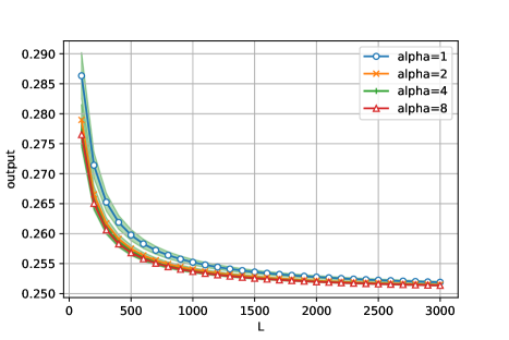
Figure 1: Average output of RNTK for random input $\boldsymbol{x},\boldsymbol{x}^{\prime}\in\mathrm{Uniform}(\mathbb{S}^{2})$ with increasing $L$

Results show that the random output is closer to $1/4$ as $L$ increases and is very close to $1/4$ when $L=3000$, which match the theoretically results in Theorem 1.

4.2 Criteria for choice of $\alpha$

In this subsection, we illustrate that the criteria for choosing $\alpha$ provided in this paper is beneficial to the generalization ability of ResNet. To this end, we demonstrate the generalization properties of kernel regression using gradient descent based on RNTK with $\alpha=1$ and $\alpha=L^{-1}$ on both synthetic data and real data. All of these results show that the test error of $\alpha=L^{-1}$ is significantly smaller than the test error of $\alpha=1$. These show that the criteria for choosing $\alpha$ provide in this paper can provide guideline in practice.

4.2.1 Synthetic data on RNTK

We first study the synthetic data $(\boldsymbol{X},Y)$ gennerated by the following model:

$$Y =\langle\boldsymbol{X},\boldsymbol{\beta}\rangle+0.1\cdot\epsilon,~{}\boldsymbol{X}\sim\mathrm{Uniform}(\mathbb{S}^{2});$$

$$\boldsymbol{\beta} =(1,1,1)^{\top},\quad\epsilon\sim N(0,1).$$

We randomly generate $200$ samples from above distribution and choose $160$ samples as training set and remaining $40$ as test set. Figure 2 plots the test error of kernel ridge regression based on RNTK using gradient descent of $\alpha=1$ or $\alpha=L^{-1}$. We show the error as a function of epoch (learning rate is set to be $0.0001$) for $L=50$ in the left subfigure and $L=200$ in right subfigure.

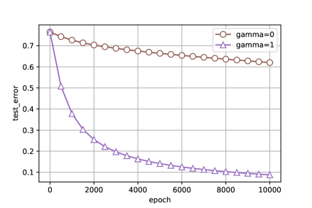
(a) $L=50$

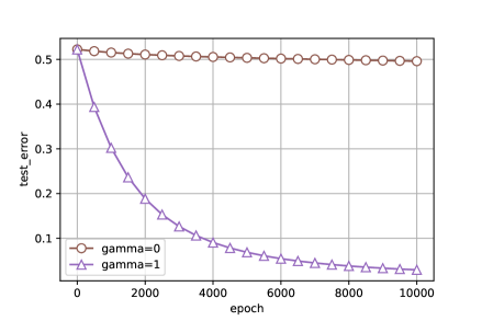
(b) $L=200$

Figure 2: Test error for synthetic data from $\mathrm{Uniform}(\mathbb{S}^{2})$ with different $\alpha$

Results show that no matter how the $t$ varies, the test error with $\alpha=L^{-1}$ is better than that with $\alpha=1$. This is consistent with our theoretical results in Section 3.

4.2.2 Real data on RNTK and ResNet

$\bullet$ RNTK: Now we study the real classification task: MNIST data and CIFAR10. We randomly choose $20000$ samples as training set and $10000$ as test set and the results for MNIST and CIFAR10 is shown in Figures 3 and 4 respectively. We plot the test error of kernel ridge regression based on RNTK using gradient descent of $\alpha=1$ or $\alpha=L^{-1}$. We show the error as a function of epoch for $L=50$ in the left subfigure and $L=200$ in right subfigure.

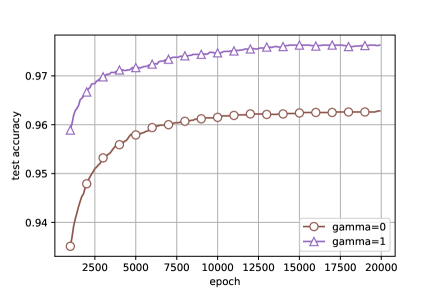
(a) MNIST,$L=50$

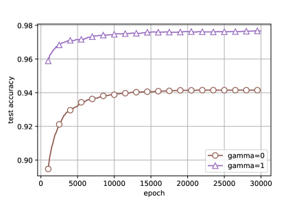
(b) MNIST,$L=200$

Figure 3: Test accuracy for MNIST $10$ with different $\alpha$

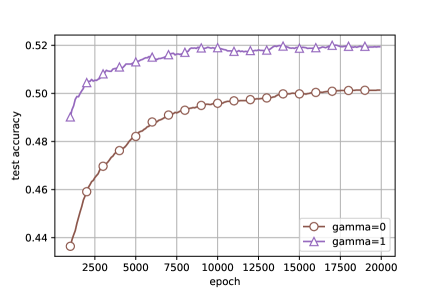
(a) CIFAR10,$L=50$

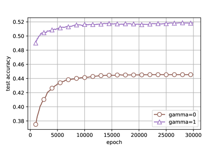
(b) CIFAR100,$L=200$

Figure 4: Test accuracy for CIFAR $10$ with different $\alpha$

Results show that no matter how the $t$ varies, the test error with $\alpha=L^{-1}$ is better than that with $\alpha=1$. This is consistent with our theoretical results in Section 3.

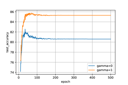
(a) CIFAR10

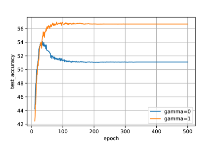
(b) CIFAR100

Figure 5: Test accuracy of ResNet with different $\alpha$. Left: CIFAR10; Right: CIFAR100

$\bullet$ ResNet: We perform the experiments on CIFAR-10 and CIFAR-100 with the convolutional residual network introduced in [12]. The first layer is $3\times 3$ convolutions with 32 filters. Then we use a stack of 16 layers with $3\times 3$ convolutions, 2 layers with 32 filters, 2 layers with 64 filters and 12 layers with 128 filters. The network ends with a global average pooling and a fully-connected layer. There are 18 stacked weighted layers in total, i.e. $L=9$. We apply the Adam to training Alex with the initial learning rate of 0.001 and the decay factor 0.95 per training epoch. The results for $\alpha=1$ and $\alpha=L^{-1}$ are reported in Figure 5.

Results show that the test accuracy with $\alpha=L^{-1}$ is better than that with $\alpha=1$. This is consistent with our theoretical results in Section 3. Furthermore, the more complex the data, the greater the improvement in accuracy caused by the selection criterion of $\alpha$ that we provide.

5 Discussion

In this paper, we propose a simple criterion for selecting $\alpha$ based on the neural tangent kernel (NTK) tool. Our findings have raised several open questions. Firstly, in Theorem 2, we only prove the large $L$ limit of RNTK when $\alpha=L^{-\gamma}$ with $\gamma=1/4$, due to the complexity of the proof. However, we believe that the conclusion in Theorem 2 holds for any $\gamma\in(0,1/2)$. Secondly, the large $L$ limit of RNTK in our paper is only pointwise. We aim to establish the simultaneous uniform convergence of ResNets with respect to both the width $m$ and depth $L$, since uniform convergence can ensure that the generalization error of infinite-depth RNTK can be well approximated by the generalization error of the large $L$ limit of RNTK.

 

Supplementary Material: Improve Generalization Ability of Deep Wide Residual Network with A Suitable Scaling Factor

 

Appendix A Preliminary

A.1 Hyper-geometric functions and Gegenbauer polynomial

Definition 2 (Falling factorial).

$\forall\lambda\in\mathbb{C}$ and $n\in\mathbb{Z}$, define

$$(\lambda)_{n}=\begin{cases}\lambda(\lambda+1)\cdots(\lambda+n-1),&n>0;\\ 1,&n=0;\\ \left[(\lambda-1)(\lambda-2)\cdots\big{(}\lambda-(-n)\big{)}\right]^{-1},&n<0.\end{cases}$$

Note that $(\lambda)_{n}$ may not exist when $n<0$. It is easy to see that for any $\lambda\in\mathbb{R}\backslash\mathbb{Z}$, $(\lambda)_{n}={\Gamma(\lambda+n)}/{\Gamma(\lambda)}$.

By definition, we can get

$$\begin{split}\frac{(2n)!}{4^{n}n!}&=\frac{(2n-1)!!(2n)!!}{4^{n}n!}=\frac{(2n-1)!!}{2^{n}}\frac{(2n)!!}{2^{n}n!}\\ &=\frac{(2n-1)!!}{2^{n}}=\frac{1}{2}\cdot\frac{3}{2}\cdot\cdots\cdot\frac{2n-1}{2}=\left(\tfrac{1}{2}\right)_{n}.\end{split}$$ (A.1)

In fact, we can also generalize the above result to

$$\frac{\Gamma(2x+1)}{4^{x}\Gamma(x+1)}=\frac{\Gamma\left(x+\frac{1}{2}\right)}{\sqrt{\pi}}~{}\text{and}~{}\frac{\Gamma(2x)}{4^{x}\Gamma(x)}=\frac{\Gamma\left(x+\frac{1}{2}\right)}{2\sqrt{\pi}}.$$ (A.2)

Definition 3 (Hypergeometric function).

The hypergeometric function is defined for $|z|<1$ by the power series

$$F(\alpha,\beta;\gamma;\boldsymbol{z})=\sum_{s=0}^{\infty}\frac{(\alpha)_{s}(\beta)_{s}}{s!(\gamma)_{s}}z^{s},$$

It is undefined (or infinite) if $\gamma$ equals a non-positive integer.

Lemma 2 (Gauss’s summation theorem).

If $\mathrm{Re}(\gamma)>\mathrm{Re}(\alpha+\beta)$, we have

$$F(\alpha,\beta;\gamma;1)=\sum_{s=0}^{\infty}\dfrac{(\alpha)_{s}(\beta)_{s}}{s!(\lambda)_{s}}=\frac{\Gamma(\gamma)\Gamma(\gamma-\alpha-\beta)}{\Gamma(\gamma-\alpha)\Gamma(\gamma-\beta)}.$$

Lemma 3.

If $\mathrm{Re}(\gamma)>\mathrm{Re}(\alpha+\beta+1)$, we have

$$\sum_{s=0}^{\infty}\dfrac{(\alpha)_{s}(\beta)_{s}(s+\mu)}{s!(\lambda)_{s}}=\frac{\Gamma(\gamma)\Gamma(\gamma-\alpha-\beta-1)}{\Gamma(\gamma-\alpha)\Gamma(\gamma-\beta)}[\mu(\gamma-\alpha-\beta-1)+\alpha\beta].$$

The Gegenbauer polynomial is defined as:

$$P_{k,d}(t)=\frac{(-1)^{k}}{2^{k}}\frac{\Gamma(\frac{d}{2})}{\Gamma(k+\frac{d}{2})}\frac{1}{(1-t^{2})^{\frac{d-2}{2}}}\frac{d^{k}}{dt^{k}}(1-t^{2})^{k-1+\frac{d}{2}}$$ (A.3)

with $d\geq 2$. It is easy to see that $P_{0,d}(t)=1,P_{1,d}(t)=t$.

Lemma 4.

$$P_{k,d}(t)=\frac{(d+k)(d+k-1)}{d(d+2k-1)}P_{k,d+2}(t)-\frac{k(k-1)}{d(d+2k-1)}P_{k-2,d+2}(t).$$

Note that [4, Theorem 4.1] have shown that the RNTK $r$ on $\mathbb{S}^{d-1}$ is the inner-product kernel. Thus we introduced the following useful lemma.

Lemma 5.

If $g(u)=\sum_{k\geq 0}c_{k}P_{k,d}(u)$ and $f(\boldsymbol{x},\boldsymbol{x}^{\prime})$ can be expressed as $f(\boldsymbol{x},\boldsymbol{x}^{\prime})=g(u):=g(\boldsymbol{x}^{\top}\boldsymbol{x}^{\prime})$ where $\boldsymbol{x},\boldsymbol{x}^{\prime}\sim\mu_{\mathcal{X}}$, then $\lambda_{k}(f)=\frac{c_{k}\mathrm{Vol}(\mathbb{S}^{d})}{a_{k,d+1}}$ where $a_{k,d+1}:=\frac{(2k+d-1)\Gamma(k+d-1)}{k!\Gamma(d)}$.

Proof.

Assume $f(\boldsymbol{x},\boldsymbol{x}^{\prime})$ has the following Mercer decomposition:

$$f(\boldsymbol{x},\boldsymbol{x}^{\prime})=\sum_{k\geq 0}\beta_{k}\sum^{N(k,d)}_{\ell=1}Y^{\ell}_{k}(\boldsymbol{x})Y^{\ell}_{k}(\boldsymbol{x}^{\prime}),$$

then the eigenvalues of $f(\boldsymbol{x},\boldsymbol{x}^{\prime})$ are $\{\beta_{k}\}_{k\geq 0}$. Denote

$$F_{k}(\boldsymbol{x},\boldsymbol{x}^{\prime})=\sum_{i=1}^{N(k,d)}Y^{i}_{k}(\boldsymbol{x})\overline{Y^{i}_{k}}(\boldsymbol{x}^{\prime})=\sum_{i=1}^{a_{k,d+1}}Y^{i}_{k}(\boldsymbol{x})\overline{Y^{i}_{k}}(\boldsymbol{x}^{\prime}),\quad x,\boldsymbol{x}^{\prime}\in\mathbb{S}^{d},$$ (A.4)

then we have:

$$F_{k}(\sigma,\tau)=\frac{a_{k,d+1}}{\mbox{vol}(\mathbb{S}^{d})}P_{k,d}(\sigma\cdot\tau).$$ (A.5)

Thus

$$f(\boldsymbol{x},\boldsymbol{x}^{\prime}) =g(u)=\sum_{k\geq 0}c_{k}P_{k,d}(u)=\sum_{k\geq 0}c_{k}\frac{F_{k}(\sigma,\tau)}{\frac{a_{k,d+1}}{\mbox{vol}(\mathbb{S}^{d})}}$$

$$=\sum_{k\geq 0}\frac{c_{k}\mathrm{vol}(\mathbb{S}^{d})}{a_{k,d+1}}F_{k}(\sigma,\tau)$$

∎

A.2 Expansion of $k_{0}$ under Gegenbauer polynomials

In the following, we denote $\Gamma(\cdot),\beta(\cdot,\cdot)$ the Gamma function and beta function respectively. According to $(\ref{1/2n})$, we can get

$$\kappa_{0}(u)=\frac{1}{2}+\frac{1}{\pi}\sum_{n=0}^{\infty}\frac{(2n)!u^{2n+1}}{4^{n}(n!)^{2}(2n+1)}=\frac{1}{2}+\frac{1}{\pi}\sum_{n=0}^{\infty}\frac{\left(\frac{1}{2}\right)_{n}}{n!}\frac{u^{2n+1}}{2n+1}.$$

Lemma 6.

Denote $C_{k}^{\lambda}(u)=\frac{\Gamma(k+2\lambda)}{k!\Gamma(2\lambda)}P_{k,2\lambda+1}(u)=\frac{(2\lambda)_{k}}{k!}P_{k,2\lambda+1}(u)$, then we have

$$u^{n} =\frac{n!\Gamma(\lambda)}{2^{n}}\sum_{s=0}^{[n/2]}\dfrac{n-2s+\lambda}{s!\Gamma(n-s+\lambda+1)}C^{\lambda}_{n-2s}(u);$$

$$=\frac{n!\sqrt{\pi}}{2^{n+d-2}\Gamma(\frac{d}{2})}\sum_{s=0}^{\lfloor n/2\rfloor}\dfrac{(n-2s+\frac{d-1}{2})\Gamma(n-2s+d-1)}{s!(n-2s)!\Gamma(n-s+\frac{d+1}{2})}P_{n-2s,d}(u).$$

where $\lfloor n/2\rfloor$ stands for rounding down of $n/2$ .

As a result of this lemma, we have

$$u^{2n+1} =\frac{(2n+1)!}{2^{2n+1}}\Gamma(\lambda)\sum_{s=0}^{n}\dfrac{2n-2s+\lambda+1}{s!\Gamma(2n-s+\lambda+2)}C^{\lambda}_{2n-2s+1}(u).$$

Further we can get

$$\kappa_{0}(u) =\frac{1}{2}+\frac{1}{\pi}\sum_{n=0}^{\infty}\frac{\left(\frac{1}{2}\right)_{n}}{n!}\frac{1}{2n+1}\frac{(2n+1)!}{2^{2n+1}}\Gamma(\lambda)\sum_{s=0}^{n}\dfrac{2n-2s+\lambda+1}{s!\Gamma(2n-s+\lambda+2)}C^{\lambda}_{2n-2s+1}(u)$$

$$=\frac{1}{2}+\frac{\Gamma(\lambda)}{2\pi}\sum_{n=0}^{\infty}{\left(\tfrac{1}{2}\right)_{n}^{2}}\sum_{s=0}^{n}\dfrac{2n-2s+\lambda+1}{s!\Gamma(2n-s+\lambda+2)}C^{\lambda}_{2n-2s+1}(u).$$

Let $m=n-k$, then we have

$$\kappa_{0}(u) =\frac{1}{2}+\frac{\Gamma(\lambda)}{2\pi}\sum_{m=0}^{\infty}\sum_{s=0}^{\infty}{\left[\left(\tfrac{1}{2}\right)_{m+s}\right]^{2}}\dfrac{2m+\lambda+1}{s!\Gamma(2m+s+\lambda+2)}C^{\lambda}_{2m+1}(u)$$

$$=\frac{1}{2}+\frac{\Gamma(\lambda)}{2\pi}\sum_{m=0}^{\infty}(2m+\lambda+1)\left(\sum_{s=0}^{\infty}{}\dfrac{\left(\tfrac{1}{2}\right)_{m+s}^{2}}{s!\Gamma(2m+s+\lambda+2)}\right)C^{\lambda}_{2m+1}(u).$$

Note that

$$\left(\tfrac{1}{2}\right)_{m+s}=\frac{\Gamma\left(\frac{1}{2}+m+s\right)}{\Gamma\left(\frac{1}{2}\right)}=\frac{\Gamma\left(\frac{1}{2}+m+s\right)}{\Gamma\left(\frac{1}{2}+m\right)}\cdot\frac{\Gamma\left(\frac{1}{2}+m\right)}{\Gamma\left(\frac{1}{2}\right)}=\left(\tfrac{1}{2}+m\right)_{s}\cdot\frac{\Gamma\left(\frac{1}{2}+m\right)}{\sqrt{\pi}};$$

$$\Gamma(2m+s+\lambda+2)=\frac{\Gamma(2m+s+\lambda+2)}{\Gamma(2m+\lambda+2)}\Gamma(2m+\lambda+2)=(2m+\lambda+2)_{s}\Gamma(2m+\lambda+2),$$

so

$$\kappa_{0}(u) =\frac{1}{2}+\frac{\Gamma(\lambda)}{2\pi^{2}}\sum_{m=0}^{\infty}\frac{2m+\lambda+1}{\Gamma(2m+\lambda+2)}\left[{\Gamma\big{(}\tfrac{1}{2}+m\big{)}}\right]^{2}\left(\sum_{s=0}^{\infty}\dfrac{\left(\tfrac{1}{2}+m\right)_{s}^{2}}{s!(2m+\lambda+2)_{s}}\right)C^{\lambda}_{2m+1}(u)$$

$$=\frac{1}{2}+\frac{\Gamma(\lambda)}{2\pi^{2}}\sum_{m=0}^{\infty}\frac{\left[{\Gamma\big{(}\tfrac{1}{2}+m\big{)}}\right]^{2}}{\Gamma(2m+\lambda+1)}\left(\sum_{s=0}^{\infty}\dfrac{\left(\tfrac{1}{2}+m\right)_{s}^{2}}{s!(2m+\lambda+2)_{s}}\right)C^{\lambda}_{2m+1}(u).$$

According to Lemma 2, we can get

$$\kappa_{0}(u) =\frac{1}{2}+\frac{\Gamma(\lambda)}{2\pi^{2}}\sum_{m=0}^{\infty}\frac{\left[{\Gamma\big{(}\tfrac{1}{2}+m\big{)}}\right]^{2}}{\Gamma(2m+\lambda+1)}\dfrac{\Gamma(2m+\lambda+2)\Gamma(\lambda+1)}{\left[\Gamma\big{(}m+\lambda+\frac{3}{2}\big{)}\right]^{2}}C^{\lambda}_{2m+1}(u)$$

$$=\frac{1}{2}+\frac{\lambda}{2\pi^{2}}\sum_{m=0}^{\infty}({2m+\lambda+1})\left[\frac{{\Gamma\big{(}\tfrac{1}{2}+m\big{)}}\Gamma(\lambda)}{\Gamma\big{(}m+\lambda+\frac{3}{2}\big{)}}\right]^{2}C^{\lambda}_{2m+1}(u)$$

$$=\frac{1}{2}+\frac{\lambda}{2\pi^{2}}\sum_{m=0}^{\infty}({2m+\lambda+1})\left[\frac{{\Gamma\big{(}\tfrac{1}{2}+m\big{)}}\Gamma(\lambda)}{\Gamma\big{(}m+\lambda+\frac{3}{2}\big{)}}\right]^{2}\frac{\Gamma(2m+1+2\lambda)}{(2m+1)!\Gamma(2\lambda)}P_{2m+1,2\lambda+1}(u).$$

Let $2m+1=k$, $2\lambda+1=n$, then we have

$$\kappa_{0}(u) =\frac{1}{2}+\frac{\lambda}{2\pi^{2}}\mathop{\sum_{k=2m+1}}\limits_{m\in\mathbb{Z}_{\geqslant 0}}({2m+\lambda+1})\left[\frac{{\Gamma\big{(}\tfrac{1}{2}+m\big{)}}\Gamma(\lambda)}{\Gamma\big{(}m+\lambda+\frac{3}{2}\big{)}}\right]^{2}\frac{\Gamma(2m+1+2\lambda)}{(2m+1)!\Gamma(2\lambda)}P_{2m+1,2\lambda+1}(u)$$

$$=\frac{1}{2}+\frac{\lambda}{2\pi^{2}}\mathop{\sum_{k=2m+1}}\limits_{m\in\mathbb{Z}_{\geqslant 0}}({k+\lambda})\left[\frac{{\Gamma\big{(}\tfrac{k}{2}\big{)}}\Gamma(\lambda)}{\Gamma\big{(}\frac{k}{2}+\lambda+1\big{)}}\right]^{2}\frac{\Gamma(k+2\lambda)}{k!\Gamma(2\lambda)}P_{k,2\lambda+1}(u)$$

$$\kappa_{0}(u) =\frac{1}{2}+\frac{n-1}{4\pi^{2}}\mathop{\sum_{k=2m+1}}\limits_{m\in\mathbb{Z}_{\geqslant 0}}\big{(}{\tfrac{2k+n-1}{2}}\big{)}\left[\frac{{\Gamma\big{(}\tfrac{k}{2}\big{)}}\Gamma\big{(}\frac{n-1}{2}\big{)}}{\Gamma\big{(}\frac{k+n+1}{2}\big{)}}\right]^{2}\frac{\Gamma(k+n-1)}{k!\Gamma(n-1)}P_{k,n}(u).$$

Note that

$$a_{k,n+1} =\frac{(n+k)!}{n!k!}-\frac{(n-k-2)!}{n!(k-2)!}=\frac{(n+k-2)!(n+k-1)(n+k)}{n!k!}-\frac{(n-k-2)!(k-1)k}{n!k!}$$

$$=\frac{(n+k-2)!}{n!k!}[(n+k-1)(n+k)-k(k-1)]=\frac{n(n+k-2)!}{n!k!}(2k+n-1)$$

$$=\frac{(n+k-2)!}{(n-1)!k!}(2k+n-1)=\frac{2k+n-1}{n-1}\frac{\Gamma(n+k-1)}{k!\Gamma(n-1)},$$

we can get

$$\kappa_{0}(u) =\frac{1}{2}+\frac{1}{2\pi^{2}}\mathop{\sum_{k=2m+1}}\limits_{m\in\mathbb{Z}_{\geqslant 0}}a_{k,n+1}\left[\frac{{\Gamma\big{(}\tfrac{k}{2}\big{)}}\Gamma\big{(}\frac{n+1}{2}\big{)}}{\Gamma\big{(}\frac{k+n+1}{2}\big{)}}\right]^{2}P_{k,n}(u)$$

$$=\frac{1}{2}+\frac{1}{2\pi^{2}}\mathop{\sum_{k=2m+1}}\limits_{m\in\mathbb{Z}_{\geqslant 0}}a_{k,n+1}\left[B\big{(}\tfrac{k}{2},\tfrac{n+1}{2}\big{)}\right]^{2}P_{k,n}(u)$$

where $B(\cdot,\cdot)$ denotes the beta function.

A.3 Expansion of $k_{1}$ under Gegenbauer polynomials

First of all, we have

$$\kappa_{1}(u) =\frac{1}{\pi}+\frac{u}{2}+\frac{1}{2\pi}\sum_{n=0}^{\infty}\frac{(2n)!}{4^{n}(n!)(n+1)!}\frac{u^{2n+2}}{2n+1}=\frac{1}{\pi}+\frac{u}{2}+\frac{1}{2\pi}\sum_{n=0}^{\infty}\frac{\left(\frac{1}{2}\right)_{n}}{(n+1)!}\frac{u^{2n+2}}{2n+1}.$$

It’s easy to see that $\big{(}\frac{1}{2}\big{)}_{-1}=\textnormal{-2}$, which means that $\left.\frac{1}{2\pi}\dfrac{\left(\frac{1}{2}\right)_{n}}{(n+1)!}\dfrac{u^{2n+2}}{2n+1}\right|_{n=\textnormal{-1}}=\frac{1}{\pi}$, then we can get

$$\kappa_{1}(u) =\frac{u}{2}+\frac{1}{2\pi}\sum_{n=-1}^{\infty}\frac{\left(\frac{1}{2}\right)_{n}}{(n+1)!}\frac{u^{2n+2}}{2n+1}=\frac{u}{2}+\frac{1}{2\pi}\sum_{n=0}^{\infty}\frac{\left(\frac{1}{2}\right)_{n-1}}{(n)!}\frac{u^{2n}}{2n-1};$$

$$u^{2n} =\frac{(2n)!\Gamma(\lambda)}{2^{2n}}\sum_{s=0}^{n}\dfrac{2n-2s+\lambda}{s!\Gamma(2n-s+\lambda+1)}C^{\lambda}_{2n-2s}(u),$$

and $\frac{(2n)!}{2^{2n}n!(2n-1)}=\frac{1}{2}\left(\frac{1}{2}\right)_{n-1}$. Based on these results, we have

$$\kappa_{1}(u) =\frac{u}{2}+\frac{\Gamma(\lambda)}{4\pi}\sum_{n=0}^{\infty}{\left(\tfrac{1}{2}\right)^{2}_{n-1}}\sum_{s=0}^{n}\dfrac{2n-2s+\lambda}{s!\Gamma(2n-s+\lambda+1)}C^{\lambda}_{2n-2s}(u).$$

Let $m=n-s$, we can get

$$\kappa_{1}(u) =\frac{u}{2}+\frac{\Gamma(\lambda)}{4\pi}\sum_{m=0}^{\infty}\sum_{s=0}^{\infty}\dfrac{{\left(\tfrac{1}{2}\right)^{2}_{m+s-1}}(2m+\lambda)}{s!\Gamma(2m+s+\lambda+1)}C^{\lambda}_{2m}(u)$$

$$=\frac{u}{2}+\frac{\Gamma(\lambda)}{4\pi^{2}}\sum_{m=0}^{\infty}\frac{(2m+\lambda)\left[\Gamma\big{(}m-\tfrac{1}{2}\big{)}\right]^{2}}{\Gamma(2m+\lambda+1)}\sum_{s=0}^{\infty}\dfrac{{\left(m-\tfrac{1}{2}\right)^{2}_{s}}}{s!(2m+\lambda+1)_{s}}C^{\lambda}_{2m}(u)$$

$$=\frac{u}{2}+\frac{\Gamma(\lambda)}{4\pi^{2}}\sum_{m=0}^{\infty}\frac{(2m+\lambda)\left[\Gamma\big{(}m-\tfrac{1}{2}\big{)}\right]^{2}}{\Gamma(2m+\lambda+1)}\frac{\Gamma(2m+\lambda+1)\Gamma(\lambda+2)}{\left[\Gamma\big{(}m+\lambda+\frac{3}{2}\big{)}\right]^{2}}C^{\lambda}_{2m}(u)$$

$$=\frac{u}{2}+\frac{\lambda(\lambda+1)}{4\pi^{2}}\sum_{m=0}^{\infty}(2m+\lambda)\left[\frac{\Gamma\big{(}m-\tfrac{1}{2}\big{)}\Gamma(\lambda)}{\Gamma\big{(}m+\lambda+\frac{3}{2}\big{)}}\right]^{2}C^{\lambda}_{2m}(u).$$

Let $2m=k$, $2\lambda+1=n$, then we have

$$\kappa_{1}(u) =\frac{u}{2}+\frac{n^{2}-1}{16\pi^{2}}\mathop{\sum_{k=2m}^{\infty}}\limits_{m\in\mathbb{Z}_{\geqslant 0}}\left(k+\tfrac{n-1}{2}\right)\left[\frac{\Gamma\big{(}\tfrac{k-1}{2}\big{)}\Gamma\big{(}\frac{n-1}{2}\big{)}}{\Gamma\big{(}\frac{k+n+2}{2}\big{)}}\right]^{2}C^{\frac{n-1}{2}}_{k}(u)$$

$$=\frac{u}{2}+\frac{n^{2}-1}{16\pi^{2}}\mathop{\sum_{k=2m}^{\infty}}\limits_{m\in\mathbb{Z}_{\geqslant 0}}\left(k+\tfrac{n-1}{2}\right)\left[\frac{\Gamma\big{(}\tfrac{k-1}{2}\big{)}\Gamma\big{(}\frac{n-1}{2}\big{)}}{\Gamma\big{(}\frac{k+n+2}{2}\big{)}}\right]^{2}\frac{\Gamma(k+n-1)}{k!\Gamma(n-1)}P_{k,n}(u)$$

$$=\frac{u}{2}+\frac{n^{2}-1}{16\pi^{2}}\mathop{\sum_{k=2m}^{\infty}}\limits_{m\in\mathbb{Z}_{\geqslant 0}}\left(k+\tfrac{n-1}{2}\right)\left[\frac{\Gamma\big{(}\tfrac{k-1}{2}\big{)}\Gamma\big{(}\frac{n-1}{2}\big{)}}{\Gamma\big{(}\frac{k+n+2}{2}\big{)}}\right]^{2}\frac{(n-1)a_{k,n+1}}{2k+n-1}P_{k,n}(u)$$

$$=\frac{P_{1,n}(u)}{2}+\frac{n+1}{8\pi^{2}}\mathop{\sum_{k=2m}^{\infty}}\limits_{m\in\mathbb{Z}_{\geqslant 0}}a_{k,n+1}\left[\frac{\Gamma\big{(}\tfrac{k-1}{2}\big{)}\Gamma\big{(}\frac{n+1}{2}\big{)}}{\Gamma\big{(}\frac{k+n+2}{2}\big{)}}\right]^{2}P_{k,n}(u)$$

$$\kappa_{1}(u) =\frac{P_{1,n}(u)}{2}+\frac{1}{2\pi^{2}}\mathop{\sum_{k=2m}^{\infty}}\limits_{m\in\mathbb{Z}_{\geqslant 0}}\frac{a_{k,n+1}}{n+1}\left[B\big{(}\tfrac{k-1}{2},\tfrac{n+3}{2}\big{)}\right]^{2}P_{k,n}(u).$$

A.4 Proof of Corollary 1

From (2.4), we know that $r^{(1)}=\frac{1}{2}[\kappa_{1}(u)+u\kappa_{0}(u)]$. Then one can calculate the expansion of $u\kappa_{0}(u)$ according to the recursion formula

$$uP_{k,d}(u)=\frac{k}{2k+d-1}P_{k-1,d}(t)+\frac{k+d-1}{2k+d-1}P_{k+1,d}(t).$$

According to the calculations mentioned earlier, we have

$$u\kappa_{0}(u) =\frac{u}{2}+\frac{1}{2\pi^{2}}\mathop{\sum_{k=2m+1}}\limits_{m\in\mathbb{Z}_{\geqslant 0}}a_{k,d+1}\left[B\big{(}\tfrac{k}{2},\tfrac{d+1}{2}\big{)}\right]^{2}uP_{k,d}(u).$$

Then we can get

$$u\kappa_{0}(u) =\frac{u}{2}+\frac{1}{2\pi^{2}}\mathop{\sum_{k=2m+1}}\limits_{m\in\mathbb{Z}_{\geqslant 0}}a_{k,d+1}\left[B\big{(}\tfrac{k}{2},\tfrac{d+1}{2}\big{)}\right]^{2}\left[\tfrac{k}{2k+d-1}P_{k-1,d}(t)+\tfrac{k+d-1}{2k+d-1}P_{k+1,d}(t)\right].$$

$$=\frac{u}{2}+\frac{1}{2\pi^{2}}\mathop{\sum_{k=2m+1}}\limits_{m\in\mathbb{Z}_{\geqslant 0}}a_{k,d+1}\left[B\big{(}\tfrac{k}{2},\tfrac{d+1}{2}\big{)}\right]^{2}\frac{k}{2k+d-1}P_{k-1,d}(t)$$

$$~{}\qquad+\frac{1}{2\pi^{2}}\mathop{\sum_{k=2m+1}}\limits_{m\in\mathbb{Z}_{\geqslant 0}}a_{k,d+1}\left[B\big{(}\tfrac{k}{2},\tfrac{d+1}{2}\big{)}\right]^{2}\frac{k+d-1}{2k+d-1}P_{k+1,d}(t).$$

$$=\frac{u}{2}+\frac{1}{2\pi^{2}}\mathop{\sum_{k_{1}=2m}}\limits_{m\in\mathbb{Z}_{\geqslant 0}}a_{k_{1}+1,d+1}\left[B\big{(}\tfrac{k_{1}+1}{2},\tfrac{d+1}{2}\big{)}\right]^{2}\frac{k_{1}+1}{2k_{1}+d+1}P_{k_{1},d}(t)$$

$$~{}\qquad+\frac{1}{2\pi^{2}}\mathop{\sum_{k=2m+2}}\limits_{m\in\mathbb{Z}_{\geqslant 0}}a_{k_{2}-1,d+1}\left[B\big{(}\tfrac{k_{2}-1}{2},\tfrac{d+1}{2}\big{)}\right]^{2}\frac{k_{2}+d-2}{2k_{2}+d-3}P_{k_{2},d}(t).$$

After further calculations, we can obtain

$$u\kappa_{0}(u) =\frac{u}{2}+\frac{a_{1,d+1}}{2\pi^{2}(d+1)}\left[B\big{(}\tfrac{1}{2},\tfrac{d+1}{2}\big{)}\right]^{2}$$

$$\,\qquad+\frac{1}{2\pi^{2}}\mathop{\sum_{k=2m+2}}\limits_{m\in\mathbb{Z}_{\geqslant 0}}\left[a_{k+1,d+1}B^{2}\big{(}\tfrac{k+1}{2},\tfrac{d+1}{2}\big{)}\tfrac{k+1}{2k+d+1}+a_{k-1,d+1}B^{2}\big{(}\tfrac{k-1}{2},\tfrac{d+1}{2}\big{)}\tfrac{k+d-2}{2k+d-3}\right]P_{k,d}(u).$$

Thus,

$$\kappa_{1}(u)+u\kappa_{0}(u) =\frac{P_{1,d}(u)}{2}+\frac{1}{2\pi^{2}}\mathop{\sum_{k=2m}^{\infty}}\limits_{m\in\mathbb{Z}_{\geqslant 0}}\frac{a_{k,d+1}}{d+1}\left[B\big{(}\tfrac{k-1}{2},\tfrac{d+3}{2}\big{)}\right]^{2}P_{k,d}(u)+\frac{u}{2}+\frac{a_{1,d+1}}{2\pi^{2}(d+1)}B^{2}\big{(}\tfrac{1}{2},\tfrac{d+1}{2}\big{)}$$

$$\qquad+\frac{1}{2\pi^{2}}\mathop{\sum_{k=2m+2}}\limits_{m\in\mathbb{Z}_{\geqslant 0}}\Big{[}a_{k+1,d+1}B^{2}\big{(}\tfrac{k+1}{2},\tfrac{d+1}{2}\big{)}\tfrac{k+1}{2k+d+1}+a_{k-1,d+1}B^{2}\big{(}\tfrac{k-1}{2},\tfrac{d+1}{2}\big{)}\tfrac{k+d-2}{2k+d-3}\Big{]}P_{k,d}(t)$$

$$=\frac{a_{1,d+1}}{2\pi^{2}(d+1)}B^{2}\big{(}\tfrac{1}{2},\tfrac{d+1}{2}\big{)}+\frac{1}{2\pi^{2}}\frac{a_{0,d+1}}{d+1}\left[B\big{(}\tfrac{-1}{2},\tfrac{d+3}{2}\big{)}\right]^{2}+P_{1,d}(u)$$

$$\qquad+\frac{1}{2\pi^{2}}\mathop{\sum_{k=2m+2}}\limits_{m\in\mathbb{Z}_{\geqslant 0}}\Big{[}a_{k+1,d+1}B^{2}\big{(}\tfrac{k+1}{2},\tfrac{d+1}{2}\big{)}\tfrac{k+1}{2k+d+1}$$

$$\quad\qquad\qquad\qquad\qquad+a_{k-1,d+1}B^{2}\big{(}\tfrac{k-1}{2},\tfrac{d+1}{2}\big{)}\tfrac{k+d-2}{2k+d-3}+\tfrac{a_{k,d+1}}{d+1}B^{2}\big{(}\tfrac{k-1}{2},\tfrac{d+3}{2}\big{)}\Big{]}P_{k,d}(t)$$

where in the last inequality we use the fact that $P_{1,d}(u)=u$. Thus

$$r^{(1)}=\frac{a_{1,d+1}}{4\pi^{2}(d+1)}B^{2}\big{(}\tfrac{1}{2},\tfrac{d+1}{2}\big{)}+\frac{1}{4\pi^{2}}\frac{a_{0,d+1}}{d+1}\left[B\big{(}\tfrac{-1}{2},\tfrac{d+3}{2}\big{)}\right]^{2}+\frac{P_{1,d}(u)}{2}$$

$$\quad+\frac{1}{4\pi^{2}}\mathop{\sum_{k=2m+2}}\limits_{m\in\mathbb{Z}_{\geqslant 0}}\Big{[}a_{k+1,d+1}B^{2}\big{(}\tfrac{k+1}{2},\tfrac{d+1}{2}\big{)}\tfrac{k+1}{2k+d+1}+a_{k-1,d+1}B^{2}\big{(}\tfrac{k-1}{2},\tfrac{d+1}{2}\big{)}\tfrac{k+d-2}{2k+d-3}+\tfrac{a_{k,d+1}}{d+1}B^{2}\big{(}\tfrac{k-1}{2},\tfrac{d+3}{2}\big{)}\Big{]}P_{k,d}(t).$$

Then by Lemma 5, since $a_{0,d+1}=1,a_{1,d+1}=d+1,a_{k,d+1}={(2k+d-1)\Gamma(k+d-1)}/[{k!\Gamma(d)}]$, we have

$$\lambda_{1}(r^{(1)}) =\frac{\mathrm{vol}(\mathbb{S}^{d})}{2(d+1)}$$

$$\lambda_{k}(r^{(1)}) =\frac{\mathrm{vol}(\mathbb{S}^{d})}{4\pi^{2}}\left[B^{2}\big{(}\tfrac{k+1}{2},\tfrac{d+1}{2}\big{)}\tfrac{k+d-1}{2k+d-1}+B^{2}\big{(}\tfrac{k-1}{2},\tfrac{d+1}{2}\big{)}\tfrac{k}{2k+d-1}+\tfrac{1}{d+1}B^{2}\big{(}\tfrac{k-1}{2},\tfrac{d+3}{2}\big{)}\right],k=2m,m\in\mathbb{Z}_{\geq 1}.$$

Appendix B Proof of Lemma 1

Now we start to prove Lemma 1. We first prove that

Lemma 7.

$r^{(2)}$ is SPD on $\mathbb{S}^{d-1}$.

Proof.

To prove $r^{(2)}$ is SPD, we only need to prove that the following is SPD:

$$\alpha^{2}\Bigg{(}\left(1+\alpha^{2}\kappa_{0}\left(\frac{u+\alpha^{2}\kappa_{1}(u)}{1+\alpha^{2}}\right)\right)\left[\kappa_{1}(u)+u\kappa_{0}(u)\right]$$

$$\qquad+(1+\alpha^{2})\kappa_{1}\left(\frac{u+\alpha^{2}\kappa_{1}(u)}{1+\alpha^{2}}\right)+(u+\alpha^{2}\kappa_{1}(u))\kappa_{0}\left(\frac{u+\alpha^{2}\kappa_{1}(u)}{1+\alpha^{2}}\right)\Bigg{)}$$

$$\quad\geq\alpha^{2}\Big{[}u\kappa_{0}\left(\tfrac{u+\alpha^{2}\kappa_{1}(u)}{1+\alpha^{2}}\right)+\kappa_{1}(u)\Big{]}\geq\alpha^{2}\Big{[}u\kappa_{0}\left(\tfrac{\alpha^{2}\kappa_{1}(u)}{1+\alpha^{2}}\right)+\kappa_{1}(u)\Big{]}$$

where $f(\cdot,\cdot)\geq g(\cdot,\cdot)$ means $f(\cdot,\cdot)-g(\cdot,\cdot)$ is PD and the last inequality comes from the Taylor expansion of $\kappa_{0}\left(\frac{u+\alpha^{2}\kappa_{1}(u)}{1+\alpha^{2}}\right)$ and Lemma 8. Then the only thing remain to be proved is that $u\kappa_{0}\left(\frac{\alpha^{2}\kappa_{1}(u)}{1+\alpha^{2}}\right)+\kappa_{1}(u)$ is SPD:

$$\kappa_{0}\left(\frac{\alpha^{2}\kappa_{1}(u)}{1+\alpha^{2}}\right) =\frac{1}{2}+\frac{\frac{\alpha^{2}\kappa_{1}(u)}{1+\alpha^{2}}}{\pi}+\frac{(\frac{\alpha^{2}\kappa_{1}(u)}{1+\alpha^{2}})^{3}}{6\pi}+\mathrm{PD}$$

$$=\frac{1}{2}+\frac{\frac{\alpha^{2}\kappa_{1}(u)}{1+\alpha^{2}}}{\pi}+\left(\frac{\alpha^{2}}{1+\alpha^{2}}\right)^{3}\frac{\kappa_{1}(u)}{6\pi}\left(\frac{1}{\pi^{2}}+\frac{u}{\pi}+\mathrm{PD}\right)+\mathrm{PD}$$

$$=\frac{1}{2}+\left(\frac{1}{\pi}\left(\frac{\alpha^{2}}{1+\alpha^{2}}\right)+\frac{1}{6\pi^{3}}\left(\frac{\alpha^{2}}{1+\alpha^{2}}\right)^{3}\right)\kappa_{1}(u)+\left(\frac{\alpha^{2}}{1+\alpha^{2}}\right)^{3}\frac{u\kappa_{1}(u)}{6\pi^{2}}+\mathrm{PD}$$

Thus $u\kappa_{0}\left(\frac{\alpha^{2}\kappa_{1}(u)}{1+\alpha^{2}}\right)+\kappa_{1}(u)$ is SPD. ∎

Then one can prove Lemma 1 by throw away items caused by $\ell$-th ($\ell>2$) layers and then prove the remain items to be SPD in the same way as Lemma 7.

Lemma 8.

The coefficients of Maclaurin expansion of $\kappa_{0}(u),\kappa_{1}(u)$ are both non-negative.

Proof.

A direct calculation leads to that

$$\kappa_{0}(u)=\frac{1}{2}+\frac{1}{\pi}\sum_{n=0}^{\infty}\frac{(2n)!}{4^{n}(n!)^{2}(2n+1)}u^{2n+1},$$ (B.1)

and

$$\kappa_{1}(u) =\frac{1}{\pi}\left[u\left(\frac{\pi}{2}+\sum_{n=0}^{\infty}\frac{(2n)!}{4^{n}(n!)^{2}(2n+1)}u^{2n+1}\right)+1+\sum_{n=1}^{\infty}\frac{(-1)^{n-1}(2n)!}{4^{n}(n!)^{2}(2n-1)}(-1)^{n}u^{2n}\right]$$

$$=\frac{1}{\pi}+\frac{u}{2}+\frac{1}{2\pi}\sum_{n=0}^{\infty}\frac{(2n)!}{4^{n}(n!)(n+1)!}\frac{u^{2n+2}}{2n+1}.$$ (B.2)

∎

Appendix C Proof of Proposition 1

In this section, we will prove the following:

• i): Generalize Theorem 4 in [16] from $\alpha=L^{-\gamma},0.5<\gamma\leq 1$ to $\alpha=CL^{-\gamma},0\leq\gamma\leq 1$;

• ii): Generalize Proposition 3.2 in [19] from $\alpha<1$ to $\alpha=CL^{-\gamma},0\leq\gamma\leq 1$;

• iii): Generalize Proposition 3.2 in [19] from fixed $L$ to arbitrary $L$.

Note that i) and iii) can be completed by modifying original proof slightly and letting $m\geq\exp(L)$, an exponential function of $L$. We only prove ii) in the following. Specifically, we only need to generalize condition $\alpha<1$ is in [19, Lemma A.2] to arbitrary $\alpha>0$.

From the proof of [16, Theorem 3], we know that as long as $m\geq\Omega(\frac{(1+\alpha^{2})^{12\ell}(1+1/4\pi)^{12L}}{\epsilon^{12}})$, with probability at least $1-\exp\left(-\Omega(m^{5/6})\right)$, we have

$$|\|\boldsymbol{\alpha}_{0,\boldsymbol{z}}^{(l)}\|^{2}-K_{\ell}(\boldsymbol{z},\boldsymbol{z})|\leq\frac{\epsilon(1+\alpha^{2})^{\ell}}{(1+1/4\pi)^{L-\ell}}$$

for any sufficiently small $\epsilon>0$. By triangle inequality, one has

$$\|\boldsymbol{\alpha}_{0,\boldsymbol{z}}^{(l)}\|^{2}\geq(1+\alpha^{2})^{\ell}-\frac{\epsilon(1+\alpha^{2})^{\ell}}{(1+1/4\pi)^{L-\ell}}\geq\Omega(1).$$

Appendix D Proof of Theorem 1

D.1 Useful simplification when the data is on $\mathbb{S}^{d-1}$

We include an additional subscript $L$ to emphasize the dependence of $\alpha$ on $L$. Let

$$u_{\ell,L}=\frac{K_{\ell,L}}{(1+\alpha^{2})^{\ell}},~{}~{}u_{0}=K_{0}=\boldsymbol{x}^{\top}\boldsymbol{z},$$

and assume that $-1+\delta<u_{0}<1-\delta$. Following these notations, we obtain the following relation

$$u_{\ell,L}=\frac{u_{\ell-1,L}+\alpha^{2}\kappa_{1}(u_{\ell-1,L})}{1+\alpha^{2}}.$$ (D.1)

Denote by

$$P_{\ell+1,L}=B_{\ell+1,L}(1+\alpha^{2})^{-(L-\ell)}=\prod_{i=\ell}^{L-1}\frac{1+\alpha^{2}\kappa_{0}(u_{i,L})}{1+\alpha^{2}}.$$

Using these notations, RNTK on the sphere (2.4) can be written as

$$r^{(L)}=\frac{1}{2L}\sum_{\ell=1}^{L}P_{\ell+1,L}\big{(}\kappa_{1}(u_{\ell-1,L})+u_{\ell-1,L}\cdot\kappa_{0}(u_{\ell-1,L})\big{)}.$$ (D.2)

D.2 The limit of $\boldsymbol{u_{\ell,L}}$ as $\boldsymbol{\ell\to\infty}$

For $\boldsymbol{x},\tilde{\boldsymbol{x}}\in\mathbb{S}^{d-1}$, it is easy to check that $u_{\ell,L}(\boldsymbol{x},\boldsymbol{x})=u_{\ell,L}(\tilde{x},\tilde{x})=1$ for all $\ell$ and

$$r^{(L)}(\boldsymbol{x},\boldsymbol{x})=r^{(L)}(\tilde{x},\tilde{x})=\frac{1}{L}\sum_{\ell=1}^{L}\frac{\kappa_{0}(1)+\kappa_{1}(1)}{2}\prod_{i=\ell}^{L-1}\frac{1+\alpha^{2}\kappa_{0}(1)}{1+\alpha^{2}}=\frac{1}{L}\sum_{\ell=1}^{L-1}\prod_{i=\ell}^{L-1}1=1.$$

Hence we only need to study when $x\neq\tilde{x}$. Recall that we have

$$u_{\ell,L}(\boldsymbol{x},\tilde{x})=\frac{u_{\ell-1,L}(\boldsymbol{x},\tilde{x})+\alpha^{2}\kappa_{1}\big{(}u_{\ell-1,L}(\boldsymbol{x},\tilde{x})\big{)}}{1+\alpha^{2}}=\varphi_{1}\big{(}u_{\ell-1,L}(\boldsymbol{x},\tilde{x})\big{)},$$

where $\varphi_{1}(\rho)=\frac{\rho+\alpha^{2}\kappa_{1}(\rho)}{1+\alpha^{2}}$.

Lemma 9.

$\varphi_{1}:[-1,1]\to[-\frac{1}{1+\alpha^{2}},1]$ is a monotonic increasing and convex function satisfying

$$0\leq\frac{\sqrt{2}}{3\pi\beta}(1-\rho)^{\frac{3}{2}}\leq\varphi_{1}(\rho)-\rho\leq\frac{\sqrt{2}}{8\beta}(1-\rho)^{\frac{3}{2}},\qquad~{}\text{where}~{}\beta=\beta(\alpha)=\frac{1+\alpha^{2}}{2\alpha^{2}}>\frac{1}{2}$$ (D.3)

and that equality holds if and only if $\rho=1$.

Proof.

By direct calculation, we have

$$\frac{\mathrm{d}\varphi_{1}(\rho)}{\mathrm{d}\rho}=1-\frac{\arccos\rho}{2\pi\beta}>\frac{1}{1+\alpha^{2}}>0;\qquad\frac{\mathrm{d}^{2}\varphi_{1}(\rho)}{\mathrm{d}\rho^{2}}=\frac{1}{2\pi\beta\sqrt{1-\rho^{2}}}>0.$$

Therefor, $\varphi_{1}$ is a monotonic increasing and convex function.

As for $(\ref{varphipro})$, it is easy to check that the equality holds for $\rho=1$. If $\rho\not=1$, let $f(\rho)=\frac{\varphi_{1}(\rho)-\rho}{(1-\rho)^{3/2}}$, then we can get

$$f(\rho)=\frac{\varphi_{1}(\rho)-\rho}{(1-\rho)^{\frac{3}{2}}}=\frac{\sqrt{1-\rho^{2}}-\rho\arccos\rho}{\pi\beta(1-\rho)^{\frac{3}{2}}};\qquad f^{\prime}(\rho)=\frac{3\sqrt{1-\rho^{2}}-(2+\rho)\arccos\rho}{2\beta(1-\rho)^{\frac{5}{2}}}.$$

Define $g(\rho)=\frac{3\sqrt{1-\rho^{2}}}{2+\rho}-\arccos\rho$, we have $g^{\prime}(\rho)=\frac{(\rho-1)^{2}}{(\rho+2)^{2}\sqrt{1-\rho^{2}}}>0$, so $g(\rho)<g(1)=0$ and $f^{\prime}(\rho)<0$. Finally, we can get

$$\frac{\sqrt{2}}{8\beta}=\lim_{\rho\to-1}f(\rho)>f(\rho)>\lim_{\rho\to 1}f(\rho)=\frac{\sqrt{2}}{3\pi\beta},\qquad\forall\rho\in[-1,1).$$

∎

For simplicity, we use $u_{\ell}$ to denote $u_{\ell,L}(\boldsymbol{x},\tilde{x})$, where $x\neq\tilde{x}$ and $x,\tilde{x}\in\mathbb{S}^{d-1}$. Because of $u_{\ell}=\varphi_{1}(u_{\ell-1})\geq u_{\ell-1}$, we can get $\{u_{\ell}\}$ is an increasing sequence. Considering that $|u_{\ell}|\leq 1$, we have $u_{\ell}$ converges as $\ell\to\infty$. Taking the limit of both sides of $u_{\ell}=\varphi_{1}(u_{\ell-1})$, we have $u_{\ell}\to 1$ as $\ell\to\infty$.

Let $e_{\ell}=1-u_{\ell}\in[0,2]$. Since $e_{\ell-1}-e_{\ell}=u_{\ell}-u_{\ell-1}=\varphi_{1}(u_{\ell-1})-u_{\ell-1}$, we can get

$$e_{\ell-1}-\frac{\sqrt{2}}{8\beta}e_{\ell-1}^{\frac{3}{2}}\leq e_{\ell}\leq e_{\ell-1}-\frac{\sqrt{2}}{3\pi\beta}e_{\ell-1}^{\frac{3}{2}}$$

according to $(\ref{varphipro})$. Hence as $e_{\ell}\to 0$, we have $\frac{e_{\ell}}{e_{\ell-1}}\to 1$, which implies $\{u_{\ell}\}$ converges sublinearly. More precisely, we have the following results:

Lemma 10.

For each $u_{0}<1$, there exists $n_{0}=n_{0}(u_{0})>0$, such that

$$1-\frac{18\pi^{2}\beta^{2}}{(n+3\pi\beta)^{2}}\leq u_{n}\leq 1-\frac{18\pi^{2}\beta^{2}}{(n+n_{0})^{2+\frac{\log(n+n_{0})}{n+n_{0}}}},\quad\forall n\in\mathbb{Z}_{\geq 0}.$$

Proof.

For the left hand side, first we can easily check that

$$1-\frac{18\pi^{2}\beta^{2}}{(n+3\pi\beta)^{2}}\in[-1,1)\qquad~{}\text{and}\qquad~{}1-\frac{18\pi^{2}\beta^{2}}{(0+3\pi\beta)^{2}}=-1\leq u_{0}.$$

Assuming that the left hand side holds for $n$. According to $(\ref{varphipro})$ we have

$$\left(1-\frac{18\pi^{2}\beta^{2}}{(n+3\pi\beta+1)^{2}}\right)-\varphi_{1}\left(1-\frac{18\pi^{2}\beta^{2}}{(n+3\pi\beta)^{2}}\right)$$

$$\qquad\leq\left(1-\frac{18\pi^{2}\beta^{2}}{(n+3\pi\beta+1)^{2}}\right)-\left(1-\frac{18\pi^{2}\beta^{2}}{(n+3\pi\beta)^{2}}\right)-\frac{\sqrt{2}}{3\pi\beta}\left(\frac{18\pi^{2}\beta^{2}}{(n+3\pi\beta)^{2}}\right)^{\frac{3}{2}}$$

$$\qquad=\frac{-18\pi^{2}\beta^{2}(3n+9\pi\beta+2)}{(n+3\pi\beta)^{3}(n+3\pi\beta+1)^{2}}\leq 0.$$

Thus, we can get

$$u_{n+1}=\varphi_{1}(u_{n})\geq\varphi_{1}\left(1-\frac{18\pi^{2}\beta^{2}}{(n+3\pi\beta)^{2}}\right)\geq 1-\frac{18\pi^{2}\beta^{2}}{(n+3\pi\beta+1)^{2}}.$$

Hence we have the left hand side.

For the right hand side, we have, by series expansion,

$$\left(1-\frac{18\pi^{2}\beta^{2}}{(n+1)^{2+\frac{\log(n+1)}{n+1}}}\right)-\varphi_{1}\left(1-\frac{18\pi^{2}\beta^{2}}{n^{2+\frac{\log n}{n}}}\right)\sim 36\pi^{2}\beta^{2}\cdot\frac{\log n}{n^{4}},$$

which means that there exists $N$ such that when $n_{0}>N$ we can get

$$\left(1-\frac{18\pi^{2}\beta^{2}}{(n+1+n_{0})^{2+\frac{\log(n+1+n_{0})}{n+1+n_{0}}}}\right)-\varphi_{1}\left(1-\frac{18\pi^{2}\beta^{2}}{(n+n_{0})^{2+\frac{\log(n+n_{0})}{n+n_{0}}}}\right)\geq 0.$$ (D.4)

Then, by choosing $n_{0}$ such that $n_{0}>N$ and $n_{0}\geq\sqrt{\frac{18\pi^{2}\beta^{2}}{1-u_{0}}}$, we have $u_{0}\leq 1-\frac{18\pi^{2}\beta^{2}}{n_{0}^{2+\frac{\log n_{0}}{n_{0}}}}$ and $\eqref{proof: Recurrence}$. Using the mathematical induction, we can get the conclusion. ∎

In the following, let us denote by $N_{\alpha}$ a positive constant satisfying $\frac{1}{1-\left(\frac{2\beta-1}{2\beta}\right)^{1/3}}-2\leq N_{\alpha}\leq\frac{1}{1-\left(\frac{2\beta-1}{2\beta}\right)^{1/3}}-1$.

Let $F(n)=\cos\left(2\pi\beta\left(1-\left(\frac{n+N_{\alpha}}{n+N_{\alpha}+1}\right)^{3-\log^{2}L/L}\right)\right)$ and $N_{0}=N_{0}(L)$ be the unique solution of $F(n+1)=\varphi_{1}\big{(}F(n)\big{)}$. Then, we have

$$\begin{cases}F(n+1)\geq\varphi_{1}\big{(}F(n)\big{)},&n\geq N_{0};\\ F(n+1)\leq\varphi_{1}\big{(}F(n)\big{)},&n\leq N_{0}.\end{cases}$$

Lemma 11.

We have $N_{0}\in\left[\frac{9L}{2(\log L)^{2}}-\frac{\log L}{2},\frac{9L}{2(\log L)^{2}}+\frac{1}{2}(\log L)^{2}-1\right]$ when $L$ is large enough.

Proof.

By series expansion, we have

$$F\left(\frac{9L}{2(\log L)^{2}}-\frac{\log L}{2}+1\right)-\varphi_{1}\left(F\left(\frac{9L}{2(\log L)^{2}}-\frac{\log L}{2}\right)\right)\sim-\frac{32\pi^{2}\beta^{2}}{2187}\frac{(\log L)^{11}}{L^{5}}$$

and

$$F\left(\frac{9L}{2(\log L)^{2}}+\frac{1}{2}\log(L)^{2}\right)-\varphi_{1}\left(F\left(\frac{9L}{2(\log L)^{2}}+\frac{1}{2}\log(L)^{2}-1\right)\right)\sim\frac{32\pi^{2}\beta^{2}}{2187}\frac{(\log L)^{12}}{L^{5}}.$$

∎

Next we would like to find $n$ such that

$$u_{n}\leq\cos\left(2\pi\beta\left(1-\left(\frac{\frac{9L}{2(\log L)^{2}}+N_{\alpha}-\frac{\log L}{2}}{\frac{9L}{2(\log L)^{2}}+N_{\alpha}+1-\frac{\log L}{2}}\right)^{3-\frac{(\log L)^{2}}{L}}\right)\right).$$

By series expansion, we know

$$\cos\left(2\pi\beta\left(1-\left(\frac{\frac{9L}{2(\log L)^{2}}+N_{\alpha}-\frac{\log L}{2}}{\frac{9L}{2(\log L)^{2}}+N_{\alpha}+1-\frac{\log L}{2}}\right)^{3-\frac{(\log L)^{2}}{L}}\right)\right)\succeq 1-\frac{18\pi^{2}\beta^{2}}{\left(\frac{9L}{2(\log L)^{2}}-\frac{\log L}{2}\right)^{2}}.$$

Then it suffices to solve

$$1-\frac{18\pi^{2}\beta^{2}}{\left(\frac{9L}{2(\log L)^{2}}-\frac{\log L}{2}\right)^{2}}\succeq 1-\frac{18\pi^{2}\beta^{2}}{(n+n_{0})^{2+\frac{\log(n+n_{0})}{n+n_{0}}}}\geq u_{n},$$

or equivalently, to solve

$$(n+n_{0})^{2+\frac{\log(n+n_{0})}{n+n_{0}}} \preceq\left(\frac{9L}{2(\log L)^{2}}-\frac{\log L}{2}\right)^{2}.$$ (D.5)

Lemma 12.

When $L$ is large enough, $n\leq\frac{9L}{2(\log L)^{2}}-\frac{1}{2}(\log L)^{2}$ satisfies $\eqref{findn}$.

Proof.

It is a straightforward computation to check that

$$(n+n_{0})^{2+\frac{\log(n+n_{0})}{n+n_{0}}}-\left(\frac{9L}{2(\log L)^{2}}-\frac{\log L}{2}\right)^{2}$$

$$\leq \left(\frac{9L}{2(\log L)^{2}}-\frac{1}{2}(\log L)^{2}+n_{0}\right)^{2+\frac{\log\left(\frac{9L}{2(\log L)^{2}}-\frac{1}{2}(\log L)^{2}+n_{0}\right)}{\frac{9L}{2(\log L)^{2}}-\frac{1}{2}(\log L)^{2}+n_{0}}}-\left(\frac{9L}{2(\log L)^{2}}-\frac{\log L}{2}\right)^{2}$$

$$\sim -\frac{18L\log\log L}{\log L}.$$

∎

Lemma 13.

For each $u_{0}<1$, we have

$$\cos\left(2\pi\beta\left(1-\left(\frac{n+N_{\alpha}}{n+N_{\alpha}+1}\right)^{3}\right)\right) \leq u_{n}\leq\cos\left(2\pi\beta\left(1-\left(\frac{n+\log^{2}L+N_{\alpha}}{n+\log^{2}L+N_{\alpha}+1}\right)^{3-\frac{(\log L)^{2}}{L}}\right)\right),~{}\forall n\in[L].$$

when $L$ is large enough.

Proof.

For the left hand side, we can easily check that

$$\cos\left(2\pi\beta\left(1-\left(\frac{n+N_{\alpha}}{n+N_{\alpha}+1}\right)^{3}\right)\right)\leq 1-\frac{18\pi^{2}\beta^{2}}{(n+3\pi\beta)^{2}}\leq u_{n}.$$

For the right hand side, let $G(n)=\cos\left(2\pi\beta\left(1-\left(\frac{n+\log^{2}L+N_{\alpha}}{n+\log^{2}L+N_{\alpha}+1}\right)^{3-\frac{(\log L)^{2}}{L}}\right)\right)=F\big{(}n+(\log L)^{2}\big{)}$. We want to proof $u_{n}\leq G(n)$.

Let $N_{1}=N_{0}-(\log L)^{2}\in\left[\frac{9L}{2(\log L)^{2}}-\frac{1}{2}\log L-(\log L)^{2},~{}\frac{9L}{2(\log L)^{2}}-\frac{1}{2}(\log L)^{2}-1\right]$. When $n\geq N_{1}$, we have $n+(\log L)^{2}\geq N_{0}$, which means that

$$\begin{cases}G(n+1)\geq\varphi_{1}\big{(}G(n)\big{)},&n\geq N_{1};\\ G(n+1)\leq\varphi_{1}\big{(}G(n)\big{)},&n\leq N_{1}.\end{cases}$$

Let $N_{2}=\lceil N_{1}\rceil$ be the least integer greater than or equal to $N_{1}$, it is easy to see that

$$\frac{9L}{2(\log L)^{2}}-\frac{1}{2}(\log L)-(\log L)^{2}\leq N_{1}\leq N_{2}\leq N_{1}+1\leq\frac{9L}{2(\log L)^{2}}-\frac{1}{2}(\log L)^{2}.$$

Because of the monotonicity of $G(n)$ and Lemma 12, we can get

$$G(N_{2}) \geq G\left(\frac{9L}{2(\log L)^{2}}-\frac{1}{2}(\log L)-(\log L)^{2}\right)=\cos\left(2\pi\beta\left(1-\left(\frac{\frac{9L}{2(\log L)^{2}}+N_{\alpha}-\frac{\log L}{2}}{\frac{9L}{2(\log L)^{2}}+N_{\alpha}+1-\frac{\log L}{2}}\right)^{3-\frac{(\log L)^{2}}{L}}\right)\right)\geq u_{N_{2}}.$$

Assuming that $u_{n}\leq G(n)$ holds for $n=k$. If $k\geq N_{2}$, we have $k\geq N_{1}$ and

$$u_{k+1}=\varphi_{1}(u_{k})\leq\varphi_{1}(G_{k})\leq G_{k+1}.$$

Also, if $n=k\leq N_{2}$, we can get $k\leq N_{1}+1$ and

$$\varphi_{1}(u_{k-1})=u_{k}\leq G(k)\leq\varphi_{1}\big{(}G({k-1})\big{)}\Longrightarrow u_{k-1}\leq G(k-1).$$

Therefore, we have the right hand side. ∎

D.3 The limit of $\boldsymbol{r^{(L)}}$ as $\boldsymbol{L\to\infty}$

Denote $N_{L}=(\log L)^{2}+N_{\alpha}$. Because $\kappa_{0}$ is a monotonic increasing function, we have

$$\kappa_{0}\left(\cos\left(2\pi\beta\left(1-\left(\frac{n+N_{\alpha}}{n+N_{\alpha}+1}\right)^{3}\right)\right)\right) \leq\kappa_{0}(u_{n})\leq\kappa_{0}\left(\cos\left(2\pi\beta\left(1-\left(\frac{n+N_{L}}{n+N_{L}+1}\right)^{3-\frac{(\log L)^{2}}{L}}\right)\right)\right).$$

When $L$ is large enough, it is easy to see that

$$\beta\left(1-\left(\frac{n+N_{\alpha}}{n+N_{\alpha}+1}\right)^{3}\right)\in[0,1/2]~{}\text{for}~{}n\geq 0.$$

$$\beta\left(1-\left(\frac{n+N_{L}}{n+N_{L}+1}\right)^{3}\right)\in[0,1/2]~{}\text{for}~{}n\geq 0.$$

Thus

$$1-2\beta\left(1-\left(\frac{n+N_{\alpha}}{n+N_{\alpha}+1}\right)^{3}\right) \leq\kappa_{0}(u_{n})\leq 1-2\beta\left(1-\left(\frac{n+N_{L}}{n+N_{L}+1}\right)^{3-\frac{(\log L)^{2}}{L}}\right).$$

i.e.

$$\left(\frac{n+N_{\alpha}}{n+N_{\alpha}+1}\right)^{3} \leq\frac{1+\alpha^{2}\kappa_{0}(u_{n})}{1+\alpha^{2}}\leq\left(\frac{n+N_{L}}{n+N_{L}+1}\right)^{3-\frac{(\log L)^{2}}{L}}.$$

Then

$$\left(\frac{\ell+N_{\alpha}}{L+N_{\alpha}+1}\right)^{3}\leq\prod_{i=\ell}^{L}\frac{1+\alpha^{2}\kappa_{0}(u_{i-1})}{1+\alpha^{2}}\leq\left(\frac{\ell+N_{L}-1}{L+N_{L}}\right)^{3-\frac{(\log L)^{2}}{L}}.$$

For the right hand side, if we sum over $\ell$, we have

$$\frac{1}{L}\sum_{\ell=1}^{L}\left(\frac{\ell+N_{L}-1}{L+N_{L}}\right)^{3-\frac{(\log L)^{2}}{L}} \leq\frac{1}{L}\int_{1}^{L+1}\left(\frac{N_{\alpha}+N_{L}-1}{L+N_{L}}\right)^{3-\frac{(\log L)^{2}}{L}}~{}\mathrm{d}x$$

$$=\frac{(L+N_{L})^{4-\frac{(\log L)^{2}}{L}}-N_{L}^{4-\frac{(\log L)^{2}}{L}}}{L(L+N_{L})^{3-\frac{(\log L)^{2}}{L}}\left(4-\frac{(\log L)^{2}}{L}\right)}.$$

Similarly, we can get

$$\frac{1}{L}\sum_{i=1}^{L}\left(\frac{\ell+N_{\alpha}}{L+N_{\alpha}+1}\right)^{3}\geq\frac{1}{L}\int_{1}^{L}\left(\frac{x+N_{\alpha}}{L+N_{\alpha}+1}\right)^{3}~{}\mathrm{d}x=\frac{(L+N_{\alpha})^{4}-(N_{\alpha}+1)^{4}}{4L(L+N_{\alpha}+1)^{3}}.$$

Hence,

$$\frac{(L+N_{\alpha})^{4}-(N_{\alpha}+1)^{4}}{4L(L+N_{\alpha}+1)^{3}}\leq\frac{1}{L}\sum_{\ell=1}^{L}\prod_{i=\ell}^{L}\frac{1+\alpha^{2}\kappa_{0}(u_{i-1})}{1+\alpha^{2}}\leq\frac{(L+N_{L})^{4-\frac{(\log L)^{2}}{L}}-N_{L}^{4-\frac{(\log L)^{2}}{L}}}{L(L+N_{L})^{3-\frac{(\log L)^{2}}{L}}\left(4-\frac{(\log L)^{2}}{L}\right)}.$$

Taking the limit of both sides, we have

$$\lim_{L\to\infty}\frac{(L+N_{\alpha})^{4}-(N_{\alpha}+1)^{4}}{4L(L+N_{\alpha}+1)^{3}}=\lim_{L\to\infty}\frac{(L+N_{L})^{4-\frac{(\log L)^{2}}{L}}-N_{L}^{4-\frac{(\log L)^{2}}{L}}}{L(L+N_{L})^{3-\frac{(\log L)^{2}}{L}}\left(4-\frac{(\log L)^{2}}{L}\right)}=\frac{1}{4}.$$

Hence,

$$\lim_{L\to\infty}\frac{1}{L}\sum_{\ell=1}^{L}\left(\frac{\ell+N-1}{L+N}\right)^{3-\frac{(\log L)^{2}}{L}} =\lim_{L\to\infty}\frac{1}{L}\sum_{\ell=1}^{L}\left(\frac{\ell+N_{\alpha}}{L+N_{\alpha}+1}\right)^{3}$$

$$=\lim_{L\to\infty}\frac{1}{L}\sum_{\ell=1}^{L}\prod_{i=\ell}^{L}\frac{1+\alpha^{2}\kappa_{0}(u_{i-1})}{1+\alpha^{2}}=\frac{1}{4}.$$

Let $v_{\ell}=u_{\ell}\kappa_{0}(u_{\ell})+\kappa_{1}(u_{\ell})$, then

$$r^{(L)}=\frac{1}{L}\sum_{\ell=1}^{L}\frac{v_{\ell-1}}{2}\prod_{i=\ell}^{L}\frac{1+\alpha^{2}\kappa_{0}(u_{i-1})}{1+\alpha^{2}}.$$

Define $\varphi_{0}(x)=x\kappa_{0}(x)+\kappa_{1}(x)$, we can get

$$0\leq 1-\frac{v_{\ell}}{2} =\frac{1}{2}\big{(}\varphi_{0}(1)-\varphi_{0}(u_{\ell})\big{)}=\frac{\sqrt{2}}{2\pi}(1-u_{\ell})^{\frac{1}{2}}+\mathcal{O}(1-u_{\ell}).$$

Recall from previous discussion, $u_{\ell}=1-\mathcal{O}({\ell^{-2}})$. Therefore, we have $\frac{v_{\ell}}{2}=1-\mathcal{O}(\ell^{-1})$ and

$$\lim_{L\to\infty}r^{(L)} =\lim_{L\to\infty}\frac{1}{L}\sum_{\ell=1}^{L}\frac{v_{\ell-1}}{2}\prod_{i=\ell}^{L}\frac{1+\alpha^{2}\kappa_{0}(u_{i-1})}{1+\alpha^{2}}$$

$$=\lim_{L\to\infty}\frac{1}{L}\sum_{\ell=1}^{L}\prod_{i=\ell}^{L}\frac{1+\alpha^{2}\kappa_{0}(u_{i-1})}{1+\alpha^{2}}-\lim_{L\to\infty}\frac{1}{L}\sum_{\ell=1}^{L}\mathcal{O}(\ell^{-1})\prod_{i=\ell}^{L}\frac{1+\alpha^{2}\kappa_{0}(u_{i-1})}{1+\alpha^{2}}$$

$$=\frac{1}{4}-\lim_{L\to\infty}\frac{1}{L}\sum_{\ell=1}^{L}\mathcal{O}(\ell^{-1})\prod_{i=\ell}^{L}\frac{1+\alpha^{2}\kappa_{0}(u_{i-1})}{1+\alpha^{2}}.$$

Because

$$\left|\frac{1}{L}\sum_{\ell=1}^{L}\mathcal{O}(\ell^{-1})\prod_{i=\ell}^{L}\frac{1+\alpha^{2}\kappa_{0}(u_{i-1})}{1+\alpha^{2}}\right|\leq\frac{C}{L}\sum_{\ell=1}^{L}\frac{1}{\ell}\prod_{i=\ell}^{L}\frac{1+\alpha^{2}\kappa_{0}(u_{i-1})}{1+\alpha^{2}}$$

$$\qquad\leq\frac{C}{L}\sum_{\ell=1}^{L}\frac{1}{\ell}\left(\frac{\ell+N_{L}-1}{L+N_{L}}\right)^{3-\frac{(\log L)^{2}}{L}}\leq\frac{C}{L}\sum_{\ell=1}^{L}\frac{({\ell+N_{L}})^{3}}{\ell\cdot L^{3-\frac{(\log L)^{2}}{L}}}$$

$$\qquad\leq\frac{C}{L^{4-\frac{(\log L)^{2}}{L}}}\int_{1}^{L+1}\frac{({x+N_{L}})^{3}}{x}~{}\mathrm{d}x\leq\frac{\mathcal{O}(L^{3})}{L^{4-\frac{(\log L)^{2}}{L}}}=\mathcal{O}(L^{-1})\to 0,$$

we can finally get

$$\lim\limits_{L\to\infty}r^{(L)}=\frac{1}{4}.$$

Also, when $L$ is large, we have

$$\frac{(L+N_{\alpha})^{4}-(N_{\alpha}+1)^{4}}{4L(L+N_{\alpha}+1)^{3}}<\frac{1}{4}<\frac{\left(L+N_{L}\right)^{4-\frac{(\log L)^{2}}{L}}-N_{L}^{4-\frac{(\log L)^{2}}{L}}}{L(L+N_{L})^{3-\frac{(\log L)^{2}}{L}}\left(4-\frac{(\log L)^{2}}{L}\right)}.$$

Then

$$\left|\frac{1}{L}\sum_{\ell=1}^{L}\prod_{i=\ell}^{L}\frac{1+\alpha^{2}\kappa_{0}(u_{i-1})}{1+\alpha^{2}}-\frac{1}{4}\right|\leq\left|\frac{\left(L+N_{L}\right)^{4-\frac{(\log L)^{2}}{L}}-N_{L}^{4-\frac{(\log L)^{2}}{L}}}{L(L+N_{L})^{3-\frac{(\log L)^{2}}{L}}\left(4-\frac{(\log L)^{2}}{L}\right)}-\frac{(L+N_{\alpha})^{4}-(N_{\alpha}+1)^{4}}{4L(L+N_{\alpha}+1)^{3}}\right|$$

$$\qquad\leq\left(\frac{\left(L+N_{L}\right)^{4-\frac{(\log L)^{2}}{L}}-N_{L}^{4-\frac{(\log L)^{2}}{L}}}{L(L+N_{L})^{3-\frac{(\log L)^{2}}{L}}\left(4-\frac{(\log L)^{2}}{L}\right)}-\frac{1}{4}\right)+\left(\frac{1}{4}-\frac{(L+N_{\alpha})^{4}-(N_{\alpha}+1)^{4}}{4L(L+N_{\alpha}+1)^{3}}\right)$$

$$\qquad\lesssim\frac{4N_{L}+(\log L)^{2}+4}{16L}.$$

Finally we can estimate the convergence rate of the kernel

$$\left|\frac{1}{L}\sum_{\ell=1}^{L}\frac{v_{\ell-1}}{2}\prod_{i=\ell}^{L}\frac{1+\alpha^{2}\kappa_{0}(u_{i-1})}{1+\alpha^{2}}-\frac{1}{4}\right|=\left|\frac{1}{L}\sum_{\ell=1}^{L}\big{(}1-\mathcal{O}(\ell^{-1})\big{)}\prod_{i=\ell}^{L}\frac{1+\alpha^{2}\kappa_{0}(u_{i-1})}{1+\alpha^{2}}-\frac{1}{4}\right|$$

$$\qquad=\left|\frac{1}{L}\sum_{\ell=1}^{L}\prod_{i=\ell}^{L}\frac{1+\alpha^{2}\kappa_{0}(u_{i-1})}{1+\alpha^{2}}-\frac{1}{4}\right|+\left|\frac{1}{L}\sum_{\ell=1}^{L}\mathcal{O}(\ell^{-1})\prod_{i=\ell}^{L}\frac{1+\alpha^{2}\kappa_{0}(u_{i-1})}{1+\alpha^{2}}\right|$$

$$\qquad\lesssim\frac{4N_{L}+(\log L)^{2}+4}{16L}+\mathcal{O}(L^{-1})=\mathcal{O}\left(\frac{\mathrm{poly}\log(L)}{L}\right).$$

Appendix E Proof of Theorem 2

In the following, let us denote $N_{\alpha}=3L^{2\gamma}$ on $\alpha=L^{-\frac{1}{4}}$ satisfying

$$\frac{1}{1-\left(\frac{2\beta-1}{2\beta}\right)^{1/3}}-2\leq N_{\alpha}\leq\frac{1}{1-\left(\frac{2\beta-1}{2\beta}\right)^{1/3}}-1$$

when $L$ is large enough.

Let $F(n)=\cos\left(2\pi\beta\left(1-\left(\frac{n+N_{\alpha}}{n+N_{\alpha}+1}\right)^{3-\log^{2}L/L}\right)\right)$ and $N_{0}=N_{0}(L)$ be the unique solution of $F(n+1)=\varphi_{1}\big{(}F(n)\big{)}$. Then, we have

$$\begin{cases}F(n+1)\geq\varphi_{1}\big{(}F(n)\big{)},&n\geq N_{0};\\ F(n+1)\leq\varphi_{1}\big{(}F(n)\big{)},&n\leq N_{0}.\end{cases}$$

Lemma 14.

We have $N_{0}\in\left[\frac{3\sqrt{5}\pi L}{5\log L},\frac{3\sqrt{5}\pi L}{5\log L}+\frac{3\sqrt{5}\pi L}{4\log^{2}L}-1\right]$ when $L$ is large enough.

Proof.

By series expansion, we have

$$F\left(\frac{3\sqrt{5}\pi L}{5\log L}+1\right)-\varphi_{1}\left(F\left(\frac{3\sqrt{5}\pi L}{5\log L}\right)\right)\sim-\frac{25}{6\pi^{2}}\frac{(\log L)^{4}}{L^{3}}$$

and

$$F\left(\frac{3\sqrt{5}\pi L}{5\log L}+\frac{3\sqrt{5}\pi L}{4\log^{2}L}\right)-\varphi_{1}\left(F\left(\frac{3\sqrt{5}\pi L}{5\log L}+\frac{3\sqrt{5}\pi L}{4\log^{2}L}-1\right)\right)\asymp\frac{51200\log^{10}(L)}{3\pi(4\log(L)+5)^{6}L^{3}}(\frac{\sqrt{5}}{3}-\frac{1}{\pi}).$$

∎

Next we would like to find $n$ such that

$$u_{n}\leq\cos\left(2\pi\beta\left(1-\left(\frac{\frac{3\sqrt{5}\pi L}{5\log L}+N_{\alpha}}{\frac{3\sqrt{5}\pi L}{5\log L}+N_{\alpha}+1}\right)^{3-\frac{(\log L)^{2}}{L}}\right)\right).$$

By series expansion, we know

$$\cos\left(2\pi\beta\left(1-\left(\frac{\frac{3\sqrt{5}\pi L}{5\log L}+N_{\alpha}}{\frac{3\sqrt{5}\pi L}{5\log L}+N_{\alpha}+1}\right)^{3-\frac{(\log L)^{2}}{L}}\right)\right)\succeq 1-\frac{18\pi^{2}\beta^{2}}{\left(\frac{3\sqrt{5}\pi L}{5\log L}+N_{\alpha}\right)^{2}}.$$

Then it suffices to solve

$$1-\frac{18\pi^{2}\beta^{2}}{\left(\frac{3\sqrt{5}\pi L}{5\log L}+N_{\alpha}\right)^{2}}\succeq 1-\frac{18\pi^{2}\beta^{2}}{(n+n_{0})^{2+\frac{\log(n+n_{0})}{n+n_{0}}}}\geq u_{n},$$

or equivalently, to solve

$$(n+n_{0})^{2+\frac{\log(n+n_{0})}{n+n_{0}}} \preceq\left(\frac{3\sqrt{5}\pi L}{5\log L}+N_{\alpha}\right)^{2}.$$ (E.1)

Lemma 15.

When $L$ is large enough, $n\leq\frac{3\sqrt{5}\pi L}{5\log L}$ satisfies $\eqref{findn:gamma0.25}$.

Proof.

It is a straightforward computation to check that

$$(n+n_{0})^{2+\frac{\log(n+n_{0})}{n+n_{0}}}-\left(\frac{3\sqrt{5}\pi L}{5\log L}+N_{\alpha}\right)^{2}$$

$$\leq \left(\frac{3\sqrt{5}\pi L}{5\log L}\right)^{2+\frac{\log\left(\frac{3\sqrt{5}\pi L}{5\log L}+n_{0}\right)}{\frac{3\sqrt{5}\pi L}{5\log L}+n_{0}}}-\left(\frac{3\sqrt{5}\pi L}{5\log L}+N_{\alpha}\right)^{2}$$

$$\sim -\frac{6\sqrt{5}\pi L^{3/2}}{6\log L}.$$

∎

Lemma 16.

For each $u_{0}<1$, we have

$$\cos\left(2\pi\beta\left(1-\left(\frac{n+N_{\alpha}}{n+N_{\alpha}+1}\right)^{3}\right)\right) \leq u_{n}\leq\cos\left(2\pi\beta\left(1-\left(\frac{n+\frac{3\sqrt{5}\pi L}{4\log^{2}L}+N_{\alpha}}{n+\frac{3\sqrt{5}\pi L}{4\log^{2}L}+N_{\alpha}+1}\right)^{3-\frac{(\log L)^{2}}{L}}\right)\right),~{}\forall n\in[L].$$

when $L$ is large enough.

Proof.

For the left hand side, we can easily check that

$$\cos\left(2\pi\beta\left(1-\left(\frac{n+N_{\alpha}}{n+N_{\alpha}+1}\right)^{3}\right)\right)\leq 1-\frac{18\pi^{2}\beta^{2}}{(n+3\pi\beta)^{2}}\leq u_{n}$$

For the right hand side, let $G(n)=\cos\left(2\pi\beta\left(1-\left(\frac{n+\frac{3\sqrt{5}\pi L}{4\log^{2}L}+N_{\alpha}}{n+\frac{3\sqrt{5}\pi L}{4\log^{2}L}+N_{\alpha}+1}\right)^{3-\frac{(\log L)^{2}}{L}}\right)\right)=F\big{(}n+\frac{3\sqrt{5}\pi L}{4\log^{2}L}\big{)}$. We want to proof $u_{n}\leq G(n)$.

Let $N_{1}=N_{0}-\frac{3\sqrt{5}\pi L}{4\log^{2}L}\in\left[\frac{3\sqrt{5}\pi L}{5\log L}-\frac{3\sqrt{5}\pi L}{4\log^{2}L},\frac{3\sqrt{5}\pi L}{5\log L}-1\right]$. When $n\geq N_{1}$, we have $n+\frac{3\sqrt{5}\pi L}{4\log^{2}L}\geq N_{0}$, which means that

$$\begin{cases}G(n+1)\geq\varphi_{1}\big{(}G(n)\big{)},&n\geq N_{1};\\ G(n+1)\leq\varphi_{1}\big{(}G(n)\big{)},&n\leq N_{1}.\end{cases}$$

Let $N_{2}=\lceil N_{1}\rceil$ be the least integer greater than or equal to $N_{1}$, it is easy to see that

$$\frac{3\sqrt{5}\pi L}{5\log L}-\frac{3\sqrt{5}\pi L}{4\log^{2}L}\leq N_{1}\leq N_{2}\leq N_{1}+1\leq\frac{3\sqrt{5}\pi L}{5\log L}.$$

Because of the monotonicity of $G(n)$ and Lemma 15, we can get

$$G(N_{2}) \geq G\left(\frac{3\sqrt{5}\pi L}{5\log L}-\frac{3\sqrt{5}\pi L}{4\log^{2}L}\right)=\cos\left(2\pi\beta\left(1-\left(\frac{\frac{3\sqrt{5}\pi L}{5\log L}+N_{\alpha}}{\frac{3\sqrt{5}\pi L}{5\log L}+N_{\alpha}+1}\right)^{3-\frac{(\log L)^{2}}{L}}\right)\right)\geq u_{N_{2}}.$$

Assuming that $u_{n}\leq G(n)$ holds for $n=k$. If $k\geq N_{2}$, we have $k\geq N_{1}$ and

$$u_{k+1}=\varphi_{1}(u_{k})\leq\varphi_{1}(G_{k})\leq G_{k+1}.$$

Also, if $n=k\leq N_{2}$, we can get $k\leq N_{1}+1$ and

$$\varphi_{1}(u_{k-1})=u_{k}\leq G(k)\leq\varphi_{1}\big{(}G({k-1})\big{)}\Longrightarrow u_{k-1}\leq G(k-1).$$

Therefore, we have the right hand side. ∎

Then as the same reasoning of Section D.3, we can complete the proof by letting $N_{L}=\frac{3\sqrt{5}\pi L}{4\log^{2}L}+N_{\alpha}$.

References

- [1] Zeyuan Allen-Zhu, Yuanzhi Li, and Zhao Song. A convergence theory for deep learning via over-parameterization. In International Conference on Machine Learning, pages 242–252. PMLR, 2019.
- [2] Sanjeev Arora, Simon S. Du, Wei Hu, Zhiyuan Li, Russ R Salakhutdinov, and Ruosong Wang. On Exact Computation with an Infinitely Wide Neural Net. In Advances in Neural Information Processing Systems, volume 32. Curran Associates, Inc., 2019.
- [3] David Balduzzi, Marcus Frean, Lennox Leary, JP Lewis, Kurt Wan-Duo Ma, and Brian McWilliams. The shattered gradients problem: If resnets are the answer, then what is the question? In International Conference on Machine Learning, pages 342–350. PMLR, 2017.
- [4] Yuval Belfer, Amnon Geifman, Meirav Galun, and Ronen Basri. Spectral analysis of the neural tangent kernel for deep residual networks. arXiv preprint arXiv:2104.03093, 2021.
- [5] Gilles Blanchard and Nicole Mücke. Optimal Rates for Regularization of Statistical Inverse Learning Problems. Foundations of Computational Mathematics, 18(4):971–1013, August 2018.
- [6] Andrea Caponnetto and Ernesto De Vito. Optimal rates for the regularized least-squares algorithm. Foundations of Computational Mathematics, 7(3):331–368, 2007.
- [7] Lénaïc Chizat, Edouard Oyallon, and Francis Bach. On Lazy Training in Differentiable Programming. In Advances in Neural Information Processing Systems, volume 32. Curran Associates, Inc., 2019.
- [8] Simon Du, Jason Lee, Haochuan Li, Liwei Wang, and Xiyu Zhai. Gradient descent finds global minima of deep neural networks. In International conference on machine learning, pages 1675–1685. PMLR, 2019.
- [9] Spencer Frei, Yuan Cao, and Quanquan Gu. Algorithm-dependent generalization bounds for overparameterized deep residual networks. Advances in neural information processing systems, 32, 2019.
- [10] Daniel Greenfeld, Meirav Galun, Ronen Basri, Irad Yavneh, and Ron Kimmel. Learning to optimize multigrid pde solvers. In International Conference on Machine Learning, pages 2415–2423. PMLR, 2019.
- [11] Moritz Hardt and Tengyu Ma. Identity matters in deep learning. arXiv preprint arXiv:1611.04231, 2016.
- [12] Kaiming He, Xiangyu Zhang, Shaoqing Ren, and Jian Sun. Deep residual learning for image recognition. In Proceedings of the IEEE conference on computer vision and pattern recognition, pages 770–778, 2016.
- [13] Kaiming He, Xiangyu Zhang, Shaoqing Ren, and Jian Sun. Identity mappings in deep residual networks. In European conference on computer vision, pages 630–645. Springer, 2016.
- [14] Andrew Howard, Mark Sandler, Grace Chu, Liang-Chieh Chen, Bo Chen, Mingxing Tan, Weijun Wang, Yukun Zhu, Ruoming Pang, Vijay Vasudevan, et al. Searching for mobilenetv3. In Proceedings of the IEEE/CVF International Conference on Computer Vision, pages 1314–1324, 2019.
- [15] Wei Hu, Zhiyuan Li, and Dingli Yu. Simple and effective regularization methods for training on noisily labeled data with generalization guarantee. arXiv preprint arXiv:1905.11368, 2019.
- [16] Kaixuan Huang, Yuqing Wang, Molei Tao, and Tuo Zhao. Why do deep residual networks generalize better than deep feedforward networks?–a neural tangent kernel perspective. arXiv preprint arXiv:2002.06262, 2020.
- [17] Arthur Jacot, Franck Gabriel, and Clement Hongler. Neural tangent kernel: Convergence and generalization in neural networks. In S. Bengio, H. Wallach, H. Larochelle, K. Grauman, N. Cesa-Bianchi, and R. Garnett, editors, Advances in Neural Information Processing Systems, volume 31. Curran Associates, Inc., 2018.
- [18] Jianfa Lai, Manyun Xu, Rui Chen, and Qian Lin. Generalization ability of wide neural networks on . arXiv preprint arXiv:2302.05933, 2023.
- [19] Jianfa Lai, Zixiong Yu, Songtao Tian, and Qian Lin. Generalization ability of wide residual networks, 2023.
- [20] Jaehoon Lee, Lechao Xiao, Samuel Schoenholz, Yasaman Bahri, Roman Novak, Jascha Sohl-Dickstein, and Jeffrey Pennington. Wide neural networks of any depth evolve as linear models under gradient descent. Advances in neural information processing systems, 32:8572–8583, 2019.
- [21] Hao Li, Zheng Xu, Gavin Taylor, Christoph Studer, and Tom Goldstein. Visualizing the loss landscape of neural nets. Advances in neural information processing systems, 31, 2018.
- [22] Xingguo Li, Junwei Lu, Zhaoran Wang, Jarvis Haupt, and Tuo Zhao. On tighter generalization bound for deep neural networks: Cnns, resnets, and beyond. arXiv preprint arXiv:1806.05159, 2018.
- [23] Yicheng Li, Zixiong Yu, Guhan Chen, and Qian Lin. Statistical optimality of deep wide neural networks, 2023.
- [24] Yuanzhi Li and Yang Yuan. Convergence analysis of two-layer neural networks with relu activation. Advances in neural information processing systems, 30, 2017.
- [25] Junhong Lin, Alessandro Rudi, Lorenzo Rosasco, and Volkan Cevher. Optimal rates for spectral algorithms with least-squares regression over Hilbert spaces. Applied and Computational Harmonic Analysis, 48(3):868–890, May 2020.
- [26] Ilija Radosavovic, Raj Prateek Kosaraju, Ross Girshick, Kaiming He, and Piotr Dollár. Designing network design spaces. In Proceedings of the IEEE/CVF Conference on Computer Vision and Pattern Recognition, pages 10428–10436, 2020.
- [27] Garvesh Raskutti, Martin J Wainwright, and Bin Yu. Early stopping and non-parametric regression: an optimal data-dependent stopping rule. The Journal of Machine Learning Research, 15(1):335–366, 2014.
- [28] Ana CQ Siravenha, Mylena NF Reis, Iraquitan Cordeiro, Renan Arthur Tourinho, Bruno D Gomes, and Schubert R Carvalho. Residual mlp network for mental fatigue classification in mining workers from brain data. In 2019 8th Brazilian Conference on Intelligent Systems (BRACIS), pages 407–412. IEEE, 2019.
- [29] Ingo Steinwart and Andreas Christmann. Support vector machines. Springer Science & Business Media, 2008.
- [30] Mingxing Tan, Bo Chen, Ruoming Pang, Vijay Vasudevan, M Sandler, A Howard, and Mnasnet Le QV. platform-aware neural architecture search for mobile. 2019 ieee. In CVF Conference on Computer Vision and Pattern Recognition (CVPR), pages 2815–2823, 2019.
- [31] Tom Tirer, Joan Bruna, and Raja Giryes. Kernel-based smoothness analysis of residual networks. In Mathematical and Scientific Machine Learning, pages 921–954. PMLR, 2022.
- [32] Andreas Veit, Michael J Wilber, and Serge Belongie. Residual networks behave like ensembles of relatively shallow networks. Advances in neural information processing systems, 29, 2016.
- [33] Fei Wang, Mengqing Jiang, Chen Qian, Shuo Yang, Cheng Li, Honggang Zhang, Xiaogang Wang, and Xiaoou Tang. Residual attention network for image classification. In Proceedings of the IEEE conference on computer vision and pattern recognition, pages 3156–3164, 2017.
- [34] Xiaolong Yang, Xiaohong Jia, Dihong Gong, Dong-Ming Yan, Zhifeng Li, and Wei Liu. Larnet: Lie algebra residual network for face recognition. In International Conference on Machine Learning, pages 11738–11750. PMLR, 2021.
- [35] Yuan Yao, Lorenzo Rosasco, and Andrea Caponnetto. On early stopping in gradient descent learning. Constructive Approximation, 26(2):289–315, 2007.
- [36] Hongjian Zhan, Qingqing Wang, and Yue Lu. Handwritten digit string recognition by combination of residual network and rnn-ctc. In International conference on neural information processing, pages 583–591. Springer, 2017.
- [37] Hongyi Zhang, Yann N Dauphin, and Tengyu Ma. Residual learning without normalization via better initialization. In International Conference on Learning Representations, volume 3, page 2, 2019.
- [38] Huishuai Zhang, Da Yu, Mingyang Yi, Wei Chen, and Tie-Yan Liu. Stabilize deep resnet with a sharp scaling factor . Machine Learning, 111(9):3359–3392, 2022.