\DeclareRedundantLanguages

english,german,frenchenglish,german,ngerman,french \newconstantfamilyC symbol=C, format=\parenthezises, reset=section

On a mathematical model for tissue regeneration

Shimi Chettiparambil Mohanan Nishith Mohan and Christina Surulescu
RPTU Kaiserslautern-Landau
surulescu@mathematik.uni-kl.de
Department of Mathematics
Postfach 3049
67653 Kaiserslautern Germany
Abstract

We propose a PDE-ODE model for tissue regeneration, obtained by parabolic upscaling from kinetic transport equations written for the mesoscopic densities of mesenchymal stem cells and chondrocytes which evolve in an artificial scaffold impregnated with hyaluron. Due to the simple chosen turning kernels, the effective equations obtained on the macroscopic level are of the usual reaction-diffusion-taxis type. We prove global existence of solutions to the coupled macroscopic system and perform a stability and bifurcation analysis, which shows that the observed patterns are driven by taxis. Numerical simulations illustrate the model behavior for various tactic sensitivities and initial conditions.

1 Introduction

With the advent of treatment paradigms speaking in favor of repairing and regenerating rather than solely surgical resection of tissues [2, 16, 28, 32, 40, 45, 47], mathematical modeling of regeneration processes in the context of e.g., wound healing, bone and meniscus regeneration has received increasing attention. Here we are primarily interested in the latter application and refer e.g. to [5, 43] and references therein for comprehensive reviews concerning such or closely related models; see also the model classification in [15].

Mesenchymal stem cells have been recognized as a source of cells which can be induced to differentiate into tissue repair cells like (fibro)chondrocytes [45, 46]. Among these, adipose derived stem cells (ADSCs) are obtained from perivascular white adipose tissue and are relatively easy to isolate; moreover, they produce a higher yield of cells when compared to other adult stem cell sources, see e.g. [18]. We will develop here a mathematical model to characterize the dynamics of ADSC and chondrocyte densities under the influence of extracellular matrix (ECM) including newly formed tissue and hyaluron impregnating a non-resorbable scaffold in which the cells migrate and proliferate. Unlike [15, 14], our model does not take into account fluid mechanics and tissue deformation: we are rather interested in the patterns generated by the dynamics of involved cell populations under the said influences. The scaffold’s anisotropic structure is not addressed here - but see again [15], which provides a detailed account of it. Our model here can be seen as a simplified module of that complex, more realistic setting. We also address here the well-posedness of this simplification and prove the global existence of solutions therefor.

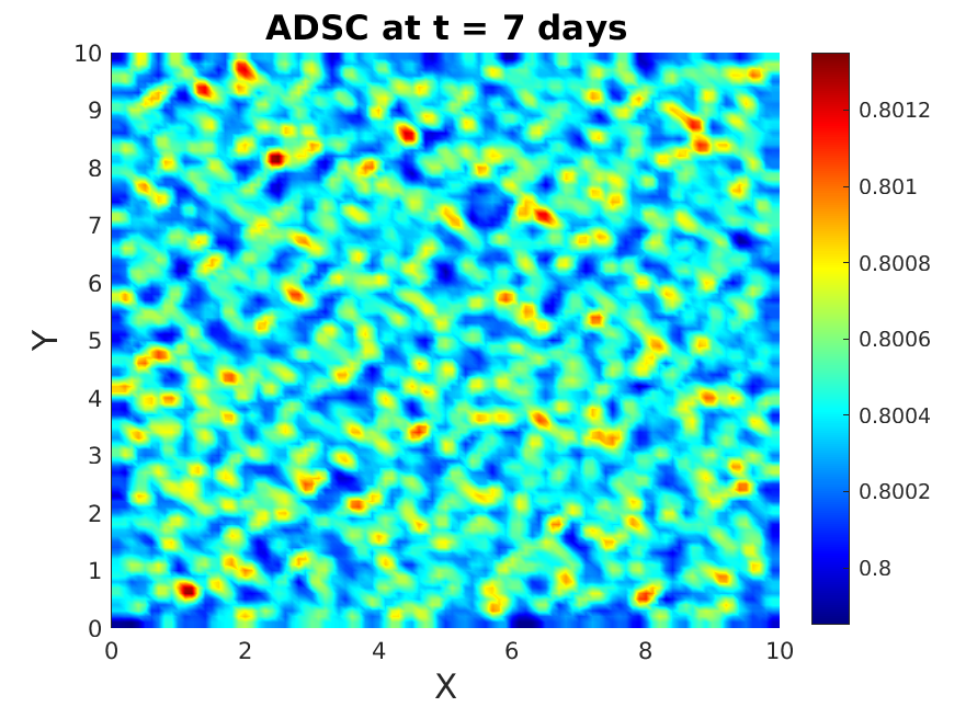
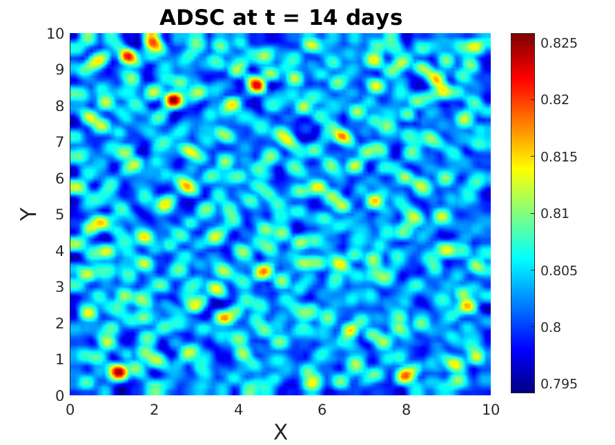
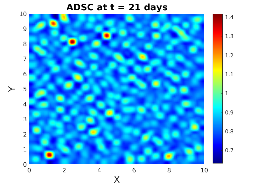
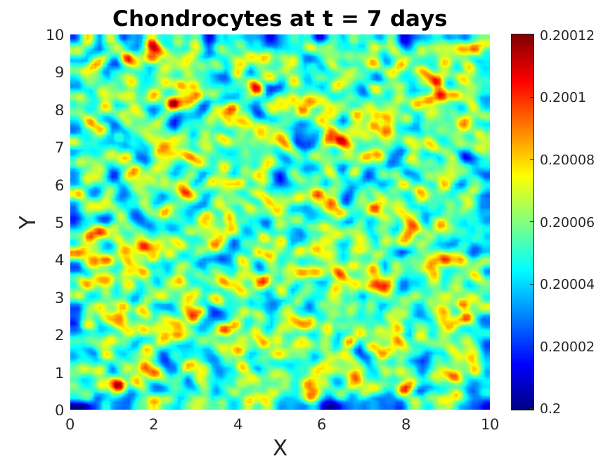
The paper is organized as follows: Section 2 is concerned with obtaining (in an informal manner) a macroscopic formulation of cell and hyaluron & ECM dynamics from decriptions on a lower (mesoscopic) scale, thus enabling us to provide some effective equations of reaction-diffusion-transport type, for which we perform in Section 3 a stability analysis of patterns and bifurcations, along with a global existence proof. Section 4 shows 1D and 2D numerical simulations of the PDE-ODE system obtained in Section 2 under various scenarios.

2 Model deduction

2.1 Mesoscopic level

We use the kinetic theory of active particles developed by Bellomo et al. [4] and describe the dynamics of cell density distributions for ADSCs and chondrocytes by way of kinetic transport equations (KTEs). Let p1(t,x,v)subscript𝑝1𝑡𝑥𝑣p_{1}(t,x,v) denote the density of ADSCs sharing at time t>0𝑡0t>0 and position xn𝑥superscript𝑛x\in{\mathbb{R}}^{n} the velocity regime vV1=s1𝕊n1𝑣subscript𝑉1subscript𝑠1superscript𝕊𝑛1v\in V_{1}=s_{1}\mathbb{S}^{n-1}. Likewise, p2(t,x,v)subscript𝑝2𝑡𝑥𝑣p_{2}(t,x,v) represents the density of chondrocytes with velocity vV2=s2𝕊n1𝑣subscript𝑉2subscript𝑠2superscript𝕊𝑛1v\in V_{2}=s_{2}\mathbb{S}^{n-1}. The positive constants s1subscript𝑠1s_{1} and s2subscript𝑠2s_{2} are the speeds of ADSCs and chondrocytes, respectively. The KTEs for p1subscript𝑝1p_{1} and p2subscript𝑝2p_{2} then write

tp1+x(vp1)=1[λ1(v,h)]p1+(de)differentiation & proliferationsubscript𝑡subscript𝑝1subscript𝑥𝑣subscript𝑝1subscript1delimited-[]subscript𝜆1𝑣subscript𝑝1(de)differentiation & proliferation\displaystyle\partial_{t}p_{1}+\nabla_{x}\cdot(vp_{1})=\mathcal{L}_{1}[\lambda_{1}(v,h)]p_{1}+\text{(de)differentiation \& proliferation} (2.1)
tp2+x(vp2)=2[λ2]p2+(de)differentiation.subscript𝑡subscript𝑝2subscript𝑥𝑣subscript𝑝2subscript2delimited-[]subscript𝜆2subscript𝑝2(de)differentiation\displaystyle\partial_{t}p_{2}+\nabla_{x}\cdot(vp_{2})=\mathcal{L}_{2}[\lambda_{2}]p_{2}+\text{(de)differentiation}. (2.2)

The first terms on the right hand sides of (2.1) and (2.2) characterize the reorientation of ADSCs and chondrocytes, respectively. The turning operators depend on the turning rates λ1subscript𝜆1\lambda_{1} and λ2subscript𝜆2\lambda_{2}, whereby the former also depends on the pathwise gradient of some ligand concentration hh, while the latter is constant:

1[λ1(v,h)]p1(t,x,v)subscript1delimited-[]subscript𝜆1𝑣subscript𝑝1𝑡𝑥𝑣\displaystyle\mathcal{L}_{1}[\lambda_{1}(v,h)]p_{1}(t,x,v) :=V1λ1(v,h)K1(v,v)p1(t,x,v)𝑑v+V1λ1(v,h)K1(v,v)p(t,x,v)𝑑vassignabsentsubscriptsubscript𝑉1subscript𝜆1𝑣subscript𝐾1superscript𝑣𝑣subscript𝑝1𝑡𝑥𝑣differential-dsuperscript𝑣subscriptsubscript𝑉1subscript𝜆1superscript𝑣subscript𝐾1𝑣superscript𝑣𝑝𝑡𝑥superscript𝑣differential-dsuperscript𝑣\displaystyle:=-\int_{V_{1}}\lambda_{1}(v,h)K_{1}(v^{\prime},v)p_{1}(t,x,v)dv^{\prime}+\int_{V_{1}}\lambda_{1}(v^{\prime},h)K_{1}(v,v^{\prime})p(t,x,v^{\prime})dv^{\prime}
=λ(v,h)p1(t,x,v)+V1λ1(v,h)K1(v,v)p(t,x,v)𝑑vabsent𝜆𝑣subscript𝑝1𝑡𝑥𝑣subscriptsubscript𝑉1subscript𝜆1superscript𝑣subscript𝐾1𝑣superscript𝑣𝑝𝑡𝑥superscript𝑣differential-dsuperscript𝑣\displaystyle=-\lambda(v,h)p_{1}(t,x,v)+\int_{V_{1}}\lambda_{1}(v^{\prime},h)K_{1}(v,v^{\prime})p(t,x,v^{\prime})dv^{\prime} (2.3)
2[λ2]p2(t,x,v)subscript2delimited-[]subscript𝜆2subscript𝑝2𝑡𝑥𝑣\displaystyle\mathcal{L}_{2}[\lambda_{2}]p_{2}(t,x,v) :=λ2p2(t,x,v)+λ2V2K2(v,v)p2(t,x,v)𝑑v.assignabsentsubscript𝜆2subscript𝑝2𝑡𝑥𝑣subscript𝜆2subscriptsubscript𝑉2subscript𝐾2𝑣superscript𝑣subscript𝑝2𝑡𝑥superscript𝑣differential-dsuperscript𝑣\displaystyle:=-\lambda_{2}p_{2}(t,x,v)+\lambda_{2}\int_{V_{2}}K_{2}(v,v^{\prime})p_{2}(t,x,v^{\prime})dv^{\prime}. (2.4)

In our model hh represents the volume fraction of an attractant ligand (hyaluron) which impregnates the fibers of an artifical scaffold on which the cells are supposed to migrate and spread. As such, it cannot diffuse or be transported, but it can be uptaken by chondrocytes and also produced by them in a limited manner. As our model does not specifically involve dynamics of newly produced extracellular matrix (ECM), nor resorption of the artificial scaffold, we lump all tissue and hyaluron volume fractions in the macroscopic variable hh. These assumptions lead for hh to the degenerate partial differential equation

th=γ1hc2+γ2c2Kc2+c2,subscript𝑡subscript𝛾1subscript𝑐2subscript𝛾2subscript𝑐2subscript𝐾subscript𝑐2subscript𝑐2\displaystyle\partial_{t}h=-\gamma_{1}hc_{2}+\gamma_{2}\frac{c_{2}}{K_{c_{2}}+c_{2}}, (2.5)

with γ1,γ2>0subscript𝛾1subscript𝛾20\gamma_{1},\gamma_{2}>0 constants.

For the turning kernels K1,K2subscript𝐾1subscript𝐾2K_{1},K_{2} we require as usual ViKi(v,v)𝑑v=1subscriptsubscript𝑉𝑖subscript𝐾𝑖𝑣superscript𝑣differential-d𝑣1\int_{V_{i}}K_{i}(v,v^{\prime})dv=1 (i=1,2𝑖12i=1,2). They can be used like e.g., in [7, 6, 8, 9, 10, 11, 12, 17, 20, 15] to account for a heterogeneous and even anisotropic environment, which is of particular relevance when a fibrous scaffold is used to support cell migration and proliferation. Here we adopt a simplified description and consider uniform turning kernels, i.e. Ki(v,v)=1/|Vi|subscript𝐾𝑖𝑣superscript𝑣1subscript𝑉𝑖K_{i}(v,v^{\prime})=1/|V_{i}| (i=1,2𝑖12i=1,2). For the turning rate of ADSCs we choose λ1(v,h)=λ0exp(ϕDth)subscript𝜆1𝑣subscript𝜆0italic-ϕsubscript𝐷𝑡\lambda_{1}(v,h)=\lambda_{0}\exp(-\phi D_{t}h), where Dth=ht+vhsubscript𝐷𝑡subscript𝑡𝑣D_{t}h=h_{t}+v\cdot\nabla h represents the pathwise gradient of hyaluron concentration hh and λ0,ϕ>0subscript𝜆0italic-ϕ0\lambda_{0},\phi>0 are constants. This choice is in line with previous works, e.g. [30, 20] related to cell migration in response to gradients of diffusing or nondiffusing cues and it typically leads to chemotactic and haptotactic behavior, respectively. With these choices the turning operators from (2.3), (2.4) become

1[λ1(v,h)]p1(t,x,v)=λ0eϕht(eϕvhp1(t,x,v)+1|V1|V1eϕvhp1(t,x,v)𝑑v)subscript1delimited-[]subscript𝜆1𝑣subscript𝑝1𝑡𝑥𝑣subscript𝜆0superscript𝑒italic-ϕsubscript𝑡superscript𝑒italic-ϕ𝑣subscript𝑝1𝑡𝑥𝑣1subscript𝑉1subscriptsubscript𝑉1superscript𝑒italic-ϕsuperscript𝑣subscript𝑝1𝑡𝑥superscript𝑣differential-dsuperscript𝑣\displaystyle\mathcal{L}_{1}[\lambda_{1}(v,h)]p_{1}(t,x,v)=\lambda_{0}e^{-\phi h_{t}}\left(-e^{-\phi v\cdot\nabla h}p_{1}(t,x,v)+\frac{1}{|V_{1}|}\int_{V_{1}}e^{-\phi v^{\prime}\cdot\nabla h}p_{1}(t,x,v^{\prime})dv^{\prime}\right)
1[λ2]p2(t,x,v)=λ2p2+λ21|V2|c2=λ2(1s2n1|𝕊n1|c2(t,x)p2(t,x,v)),subscript1delimited-[]subscript𝜆2subscript𝑝2𝑡𝑥𝑣subscript𝜆2subscript𝑝2subscript𝜆21subscript𝑉2subscript𝑐2subscript𝜆21superscriptsubscript𝑠2𝑛1superscript𝕊𝑛1subscript𝑐2𝑡𝑥subscript𝑝2𝑡𝑥𝑣\displaystyle\mathcal{L}_{1}[\lambda_{2}]p_{2}(t,x,v)=-\lambda_{2}p_{2}+\lambda_{2}\frac{1}{|V_{2}|}c_{2}=\lambda_{2}(\frac{1}{s_{2}^{n-1}|\mathbb{S}^{n-1}|}c_{2}(t,x)-p_{2}(t,x,v)), (2.6)

where ci(t,x):=Vipi(t,x,v)𝑑vassignsubscript𝑐𝑖𝑡𝑥subscriptsubscript𝑉𝑖subscript𝑝𝑖𝑡𝑥𝑣differential-d𝑣c_{i}(t,x):=\int_{V_{i}}p_{i}(t,x,v)dv (i=1,2𝑖12i=1,2) denote the macroscopic densities of ADSCs and chondrocytes, respectively. For small enough values of ϕitalic-ϕ\phi we get for 1subscript1\mathcal{L}_{1} the approximation

1[λ1(v,h)]p1(t,x,v)λ0(1ϕ(ht+vh))p1+λ0|V1|(c1ϕ(htc1+M1h)),similar-to-or-equalssubscript1delimited-[]subscript𝜆1𝑣subscript𝑝1𝑡𝑥𝑣subscript𝜆01italic-ϕsubscript𝑡𝑣subscript𝑝1subscript𝜆0subscript𝑉1subscript𝑐1italic-ϕsubscript𝑡subscript𝑐1subscript𝑀1\displaystyle\mathcal{L}_{1}[\lambda_{1}(v,h)]p_{1}(t,x,v)\simeq-\lambda_{0}\left(1-\phi(h_{t}+v\cdot\nabla h)\right)p_{1}+\frac{\lambda_{0}}{|V_{1}|}\left(c_{1}-\phi\left(h_{t}c_{1}+M_{1}\cdot\nabla h\right)\right), (2.7)

where M1(t,x):=V1vp1(t,x,v)𝑑vassignsubscript𝑀1𝑡𝑥subscriptsubscript𝑉1𝑣subscript𝑝1𝑡𝑥𝑣differential-d𝑣M_{1}(t,x):=\int_{V_{1}}vp_{1}(t,x,v)dv denotes the first moment of the ADSC orientation distribution.

Similarly to [7, 8, 12, 15] we consider the following source terms:

𝒮1p1subscript𝒮1subscript𝑝1\displaystyle\mathcal{S}_{1}p_{1} :=αp1+δp2+βp1(1c1Kc1c2Kc2),assignabsent𝛼subscript𝑝1𝛿subscript𝑝2𝛽subscript𝑝11subscript𝑐1subscript𝐾subscript𝑐1subscript𝑐2subscript𝐾subscript𝑐2\displaystyle:=-\alpha p_{1}+\delta p_{2}+\beta p_{1}(1-\frac{c_{1}}{K_{c_{1}}}-\frac{c_{2}}{K_{c_{2}}}),
𝒮2p2subscript𝒮2subscript𝑝2\displaystyle\mathcal{S}_{2}p_{2} :=αp1δp2,assignabsent𝛼subscript𝑝1𝛿subscript𝑝2\displaystyle:=\alpha p_{1}-\delta p_{2},

with α>0𝛼0\alpha>0 denoting the differentiation rate of ADSCs to chondrocytes and δ>0𝛿0\delta>0 the dedifferentiation rate of chondrocytes to ADSCs. The constant β>0𝛽0\beta>0 represents the proliferation rate of ADSCs (chondrocytes are assumed not to proliferate during the time considered here) and Kc1,Kc2>0subscript𝐾subscript𝑐1subscript𝐾subscript𝑐20K_{c_{1}},K_{c_{2}}>0 represent the carrying capacities of the two cell populations.

2.2 Parabolic upscaling

We perform a parabolic scaling of the KTEs (2.1), (2.2), i.e. we rescale the time and space variables by t~:=ε2tassign~𝑡superscript𝜀2𝑡\tilde{t}:=\varepsilon^{2}t, x~:=εxassign~𝑥𝜀𝑥\tilde{x}:=\varepsilon x. Since proliferation is much slower than migration, we also rescale as in [7, 8, 12, 15] with ε2superscript𝜀2\varepsilon^{2} the corresponding terms 𝒮1p1subscript𝒮1subscript𝑝1\mathcal{S}_{1}p_{1}, 𝒮2p2subscript𝒮2subscript𝑝2\mathcal{S}_{2}p_{2}. For notation simplification we will drop in the following the similar-to\sim symbol from the scaled variables t𝑡t and x𝑥x. Thus, we get:

ε2tp1+ε(vp1)superscript𝜀2subscript𝑡subscript𝑝1𝜀𝑣subscript𝑝1\displaystyle\varepsilon^{2}\partial_{t}p_{1}+\varepsilon\nabla\cdot(vp_{1}) =λ0(1ϕ(ε2ht+εvh))p1+λ0|V1|(c1ϕ(ε2htc1+εM1h))absentsubscript𝜆01italic-ϕsuperscript𝜀2subscript𝑡𝜀𝑣subscript𝑝1subscript𝜆0subscript𝑉1subscript𝑐1italic-ϕsuperscript𝜀2subscript𝑡subscript𝑐1𝜀subscript𝑀1\displaystyle=-\lambda_{0}\left(1-\phi(\varepsilon^{2}h_{t}+\varepsilon v\cdot\nabla h)\right)p_{1}+\frac{\lambda_{0}}{|V_{1}|}\left(c_{1}-\phi\left(\varepsilon^{2}h_{t}c_{1}+\varepsilon M_{1}\cdot\nabla h\right)\right)
+\displaystyle+ ε2(αp1+δp2+βp1(1c1Kc1c2Kc2))superscript𝜀2𝛼subscript𝑝1𝛿subscript𝑝2𝛽subscript𝑝11subscript𝑐1subscript𝐾subscript𝑐1subscript𝑐2subscript𝐾subscript𝑐2\displaystyle\varepsilon^{2}\left(-\alpha p_{1}+\delta p_{2}+\beta p_{1}(1-\frac{c_{1}}{K_{c_{1}}}-\frac{c_{2}}{K_{c_{2}}})\right)
ε2tp2+ε(vp2)superscript𝜀2subscript𝑡subscript𝑝2𝜀𝑣subscript𝑝2\displaystyle\varepsilon^{2}\partial_{t}p_{2}+\varepsilon\nabla\cdot(vp_{2}) =λ2(1|V2|c2p2)+ε2(αp1δp2).absentsubscript𝜆21subscript𝑉2subscript𝑐2subscript𝑝2superscript𝜀2𝛼subscript𝑝1𝛿subscript𝑝2\displaystyle=\lambda_{2}(\frac{1}{|V_{2}|}c_{2}-p_{2})+\varepsilon^{2}\left(\alpha p_{1}-\delta p_{2}\right).

In the sequel we consider pisubscript𝑝𝑖p_{i} (i=1,2𝑖12i=1,2) to be compactly supported in the phase space n×Visuperscript𝑛subscript𝑉𝑖{\mathbb{R}}^{n}\times V_{i}. Using Hilbert expansions of pisubscript𝑝𝑖p_{i} and identifying equal powers of ε𝜀\varepsilon we obtain:

ε0superscript𝜀0\varepsilon^{0}:

p1,0=1s1n1|𝕊n1|c1,0subscript𝑝101superscriptsubscript𝑠1𝑛1superscript𝕊𝑛1subscript𝑐10\displaystyle p_{1,0}=\frac{1}{s_{1}^{n-1}|\mathbb{S}^{n-1}|}c_{1,0} (2.8)
p2,0=1s2n1|𝕊n1|c2,0;subscript𝑝201superscriptsubscript𝑠2𝑛1superscript𝕊𝑛1subscript𝑐20\displaystyle p_{2,0}=\frac{1}{s_{2}^{n-1}|\mathbb{S}^{n-1}|}c_{2,0}; (2.9)

ε1superscript𝜀1\varepsilon^{1}:

vp1,0𝑣subscript𝑝10\displaystyle v\cdot\nabla p_{1,0} =λ0(p1,1ϕvhp1,0)+λ0|V1|(c1,1ϕM1,0h)absentsubscript𝜆0subscript𝑝11italic-ϕ𝑣subscript𝑝10subscript𝜆0subscript𝑉1subscript𝑐11italic-ϕsubscript𝑀10\displaystyle=-\lambda_{0}(p_{1,1}-\phi v\cdot\nabla hp_{1,0})+\frac{\lambda_{0}}{|V_{1}|}\left(c_{1,1}-\phi M_{1,0}\cdot\nabla h\right)
=λ0(p1,1ϕvhp1,0)+λ0|V1|c1,1(by (2.8))absentsubscript𝜆0subscript𝑝11italic-ϕ𝑣subscript𝑝10subscript𝜆0subscript𝑉1subscript𝑐11(by (2.8))\displaystyle=-\lambda_{0}(p_{1,1}-\phi v\cdot\nabla hp_{1,0})+\frac{\lambda_{0}}{|V_{1}|}c_{1,1}\quad\text{(by \eqref{ADSC:p1-c1})} (2.10)
vp2,0𝑣subscript𝑝20\displaystyle v\cdot\nabla p_{2,0} =λ2(1|V2|c2,1p2,1).absentsubscript𝜆21subscript𝑉2subscript𝑐21subscript𝑝21\displaystyle=\lambda_{2}(\frac{1}{|V_{2}|}c_{2,1}-p_{2,1}). (2.11)

With the notation [λ0]p:=λ0(1|V1|V1p(v)𝑑vp(v))assigndelimited-[]subscript𝜆0𝑝subscript𝜆01subscript𝑉1subscriptsubscript𝑉1𝑝𝑣differential-d𝑣𝑝𝑣\mathcal{L}[\lambda_{0}]p:=\lambda_{0}\left(\frac{1}{|V_{1}|}\int_{V_{1}}p(v)dv-p(v)\right) we can rewrite (2.10) as

[λ0]p1,1=λ0ϕ1|V1|c1,0vh+(vc1,0|V1|).delimited-[]subscript𝜆0subscript𝑝11subscript𝜆0italic-ϕ1subscript𝑉1subscript𝑐10𝑣𝑣subscript𝑐10subscript𝑉1\displaystyle\mathcal{L}[\lambda_{0}]p_{1,1}=-\lambda_{0}\phi\frac{1}{|V_{1}|}c_{1,0}v\cdot\nabla h+\nabla\cdot(v\frac{c_{1,0}}{|V_{1}|}). (2.12)

Since the integral with respect to v𝑣v of the right hand side in the above equation vanishes, we can invert [λ0]delimited-[]subscript𝜆0\mathcal{L}[\lambda_{0}] to obtain

p1,1=1λ0(vc1,0|V1|)+ϕ1|V1|c1,0vh.subscript𝑝111subscript𝜆0𝑣subscript𝑐10subscript𝑉1italic-ϕ1subscript𝑉1subscript𝑐10𝑣\displaystyle p_{1,1}=-\frac{1}{\lambda_{0}}\nabla\cdot(v\frac{c_{1,0}}{|V_{1}|})+\phi\frac{1}{|V_{1}|}c_{1,0}v\cdot\nabla h. (2.13)

Analogously, from (2.11) we obtain

p2,1=1λ2(vc2,0|V2|).subscript𝑝211subscript𝜆2𝑣subscript𝑐20subscript𝑉2\displaystyle p_{2,1}=-\frac{1}{\lambda_{2}}\nabla\cdot\left(v\frac{c_{2,0}}{|V_{2}|}\right). (2.14)

ε2superscript𝜀2\varepsilon^{2}:

tp1,0+(vp1,1)subscript𝑡subscript𝑝10𝑣subscript𝑝11\displaystyle\partial_{t}p_{1,0}+\nabla\cdot(vp_{1,1}) =λ0(p1,2c1,2|V1|)absentsubscript𝜆0subscript𝑝12subscript𝑐12subscript𝑉1\displaystyle=-\lambda_{0}\left(p_{1,2}-\frac{c_{1,2}}{|V_{1}|}\right)
+\displaystyle+ λ0ϕ(ht(p1,0c1,0|V1|)+vhp1,11|V1|M1,1h)subscript𝜆0italic-ϕsubscript𝑡subscript𝑝10subscript𝑐10subscript𝑉1𝑣subscript𝑝111subscript𝑉1subscript𝑀11\displaystyle\lambda_{0}\phi\left(h_{t}(p_{1,0}-\frac{c_{1,0}}{|V_{1}|})+v\cdot\nabla hp_{1,1}-\frac{1}{|V_{1}|}M_{1,1}\cdot\nabla h\right)
\displaystyle- αp1,0+δp2,0+βp1,0(1c1,0Kc1c2,0Kc2)𝛼subscript𝑝10𝛿subscript𝑝20𝛽subscript𝑝101subscript𝑐10subscript𝐾subscript𝑐1subscript𝑐20subscript𝐾subscript𝑐2\displaystyle\alpha p_{1,0}+\delta p_{2,0}+\beta p_{1,0}\left(1-\frac{c_{1,0}}{K_{c_{1}}}-\frac{c_{2,0}}{K_{c_{2}}}\right) (2.15)
tp2,0+(vp2,1)subscript𝑡subscript𝑝20𝑣subscript𝑝21\displaystyle\partial_{t}p_{2,0}+\nabla\cdot(vp_{2,1}) =λ2(1|V2|c2,2p2,2)+αp1,0δp2,0.absentsubscript𝜆21subscript𝑉2subscript𝑐22subscript𝑝22𝛼subscript𝑝10𝛿subscript𝑝20\displaystyle=\lambda_{2}(\frac{1}{|V_{2}|}c_{2,2}-p_{2,2})+\alpha p_{1,0}-\delta p_{2,0}. (2.16)

Integrating (2.15) with respect to v𝑣v and using (2.13), we obtain

tc1,0(s12nλ0c1,0)+(s12ϕnc1,0h)=αc1,0+δc2,0+βc1,0(1c1,0Kc1c2,0Kc2)subscript𝑡subscript𝑐10superscriptsubscript𝑠12𝑛subscript𝜆0subscript𝑐10superscriptsubscript𝑠12italic-ϕ𝑛subscript𝑐10𝛼subscript𝑐10𝛿subscript𝑐20𝛽subscript𝑐101subscript𝑐10subscript𝐾subscript𝑐1subscript𝑐20subscript𝐾subscript𝑐2\displaystyle\partial_{t}c_{1,0}-\nabla\cdot\left(\frac{s_{1}^{2}}{n\lambda_{0}}\nabla c_{1,0}\right)+\nabla\cdot\left(\frac{s_{1}^{2}\phi}{n}c_{1,0}\nabla h\right)=-\alpha c_{1,0}+\delta c_{2,0}+\beta c_{1,0}\left(1-\frac{c_{1,0}}{K_{c_{1}}}-\frac{c_{2,0}}{K_{c_{2}}}\right) (2.17)

Likewise, integrating (2.16) with respect to v𝑣v and using (2.14) leads to

tc2,0(s22nλ2c2,0)=αc1,0δc2,0.subscript𝑡subscript𝑐20superscriptsubscript𝑠22𝑛subscript𝜆2subscript𝑐20𝛼subscript𝑐10𝛿subscript𝑐20\displaystyle\partial_{t}c_{2,0}-\nabla\cdot\left(\frac{s_{2}^{2}}{n\lambda_{2}}\nabla c_{2,0}\right)=\alpha c_{1,0}-\delta c_{2,0}. (2.18)

The obtained equations (2.17), (2.18) describe the macroscopic dynamics of ADSC and chondrocyte densities, respectively, at leading order w.r.t. ε1much-less-than𝜀1\varepsilon\ll 1. They are supplemented with the macroscopic equation (2.5) for the dynamics of hyaluron/ECM density hh.

The above macroscopic system for ADSC and chondrocyte densities has been deduced upon considering xn𝑥superscript𝑛x\in{\mathbb{R}}^{n} and, together with (2.5), it has to be supplemented with appropriate initial conditions. Subsequently we will consider the dynamics to take place in a bounded, sufficiently regular domain ΩnΩsuperscript𝑛\Omega\subset{\mathbb{R}}^{n} and endow it with no-flux boundary conditions, which can be obtained in a similar way to that presented in [33, 8, 9]. We emphasize the fact that the obtained motility coefficients - although occurring in a macroscopic setting- depend on parameters originating on a lower (mesoscopic) scale: cell speeds s1,s2subscript𝑠1subscript𝑠2s_{1},s_{2}, turning rates λ0,λ2subscript𝜆0subscript𝜆2\lambda_{0},\lambda_{2}, and orientation bias ϕitalic-ϕ\phi towards the gradient of hh.

3 Analysis of the macroscopic model

Choosing a1:=s12nλ0assignsubscript𝑎1superscriptsubscript𝑠12𝑛subscript𝜆0a_{1}:=\frac{s_{1}^{2}}{n\lambda_{0}}, a2:=s22nλ2assignsubscript𝑎2superscriptsubscript𝑠22𝑛subscript𝜆2a_{2}:=\frac{s_{2}^{2}}{n\lambda_{2}}, and b:=s12ϕnassign𝑏superscriptsubscript𝑠12italic-ϕ𝑛b:=\frac{s_{1}^{2}\phi}{n} we consider the following macroscopic model for the dynamics of ADSCs, chondrocytes, and hyaluron/ECM:

tc1subscript𝑡subscript𝑐1\displaystyle\partial_{t}c_{1} =a1Δc1(bc1h)αc1+δc2+βc1(1c1Kc1c2Kc1),absentsubscript𝑎1Δsubscript𝑐1𝑏subscript𝑐1𝛼subscript𝑐1𝛿subscript𝑐2𝛽subscript𝑐11subscript𝑐1subscript𝐾subscript𝑐1subscript𝑐2subscript𝐾subscript𝑐1\displaystyle=a_{1}\Delta c_{1}-\nabla\cdot(bc_{1}\nabla h)-\alpha c_{1}+\delta c_{2}+\beta c_{1}(1-\frac{c_{1}}{K_{c_{1}}}-\frac{c_{2}}{K_{c_{1}}}),\leavevmode\nobreak\ \leavevmode\nobreak\ \leavevmode\nobreak\ \leavevmode\nobreak\ \leavevmode\nobreak\ \leavevmode\nobreak\ in(0,T)×Ω,in0𝑇Ω\displaystyle\text{in}\leavevmode\nobreak\ \leavevmode\nobreak\ (0,T)\times\Omega, (3.1)
tc2subscript𝑡subscript𝑐2\displaystyle\partial_{t}c_{2} =a2Δc2+αc1δc2,absentsubscript𝑎2Δsubscript𝑐2𝛼subscript𝑐1𝛿subscript𝑐2\displaystyle=a_{2}\Delta c_{2}+\alpha c_{1}-\delta c_{2},\leavevmode\nobreak\ \leavevmode\nobreak\ \leavevmode\nobreak\ \leavevmode\nobreak\ \leavevmode\nobreak\ \leavevmode\nobreak\ in(0,T)×Ω,in0𝑇Ω\displaystyle\text{in}\leavevmode\nobreak\ \leavevmode\nobreak\ (0,T)\times\Omega,
thsubscript𝑡\displaystyle\partial_{t}h =γ1hc2+γ2c2Kc2+c2,absentsubscript𝛾1subscript𝑐2subscript𝛾2subscript𝑐2subscript𝐾subscript𝑐2subscript𝑐2\displaystyle=-\gamma_{1}hc_{2}+\gamma_{2}\dfrac{c_{2}}{K_{c_{2}}+c_{2}},\leavevmode\nobreak\ \leavevmode\nobreak\ \leavevmode\nobreak\ \leavevmode\nobreak\ \leavevmode\nobreak\ \leavevmode\nobreak\ in(0,T)×Ω,in0𝑇Ω\displaystyle\text{in}\leavevmode\nobreak\ \leavevmode\nobreak\ (0,T)\times\Omega,
νc1subscript𝜈subscript𝑐1\displaystyle\partial_{\nu}c_{1} =νc2=νh=0,absentsubscript𝜈subscript𝑐2subscript𝜈0\displaystyle=\partial_{\nu}c_{2}=\partial_{\nu}h=0,\leavevmode\nobreak\ \leavevmode\nobreak\ \leavevmode\nobreak\ \leavevmode\nobreak\ \leavevmode\nobreak\ \leavevmode\nobreak\ on(0,T)×Ω,on0𝑇Ω\displaystyle\text{on}\leavevmode\nobreak\ \leavevmode\nobreak\ (0,T)\times\partial\Omega,
c1(0)subscript𝑐10\displaystyle c_{1}(0) =c10,c2(0)=c20,h(0)=h0formulae-sequenceabsentsuperscriptsubscript𝑐10formulae-sequencesubscript𝑐20superscriptsubscript𝑐200subscript0\displaystyle=c_{1}^{0},\ c_{2}(0)=c_{2}^{0},\ h(0)=h_{0} inΩ,inΩ\displaystyle\text{in}\leavevmode\nobreak\ \leavevmode\nobreak\ \Omega,

where a1,a2,α,β,γ,δ,b>0subscript𝑎1subscript𝑎2𝛼𝛽𝛾𝛿𝑏0a_{1},\ a_{2},\ \alpha,\ \beta,\ \gamma,\ \delta,\ b>0 are all positive constants and ΩnΩsuperscript𝑛\Omega\subset{\mathbb{R}}^{n} (n=2,3𝑛23n=2,3) is a bounded domain with sufficiently regular boundary, while ν𝜈\nu represents the outer unit normal on ΩΩ\partial\Omega.

3.1 Global existence

We consider model (3.1) with xΩ𝑥Ωx\in\Omega and t>0𝑡0t>0. We also assume that the initial data (c10,c20,h0)superscriptsubscript𝑐10superscriptsubscript𝑐20subscript0(c_{1}^{0},c_{2}^{0},h_{0}) satisfy for some ω(0,1)𝜔01\omega\in(0,1)

{c10(x)0,c20(x)0,h0(x)0,c10C2+ω(Ω¯),c20(x)C2+ω(Ω¯),h0(x)C2+ω(Ω¯),c10ν=c20ν=h0ν=0onΩ.casesformulae-sequencesuperscriptsubscript𝑐10𝑥0formulae-sequencesuperscriptsubscript𝑐20𝑥0subscript0𝑥0otherwiseformulae-sequencesuperscriptsubscript𝑐10superscript𝐶2𝜔¯Ωformulae-sequencesuperscriptsubscript𝑐20𝑥superscript𝐶2𝜔¯Ωsubscript0𝑥superscript𝐶2𝜔¯Ωotherwisesuperscriptsubscript𝑐10𝜈superscriptsubscript𝑐20𝜈subscript0𝜈0onΩotherwise\begin{cases}c_{1}^{0}(x)\geq 0,\ c_{2}^{0}(x)\geq 0,\ h_{0}(x)\geq 0,\\[5.0pt] c_{1}^{0}\in C^{2+\omega}(\bar{\Omega}),\ c_{2}^{0}(x)\in C^{2+\omega}(\bar{\Omega}),\ h_{0}(x)\in C^{2+\omega}(\bar{\Omega}),\\[5.0pt] \dfrac{\partial c_{1}^{0}}{\partial\nu}=\dfrac{\partial c_{2}^{0}}{\partial\nu}=\dfrac{\partial h_{0}}{\partial\nu}=0\leavevmode\nobreak\ \text{on}\leavevmode\nobreak\ \partial\Omega.\end{cases} (3.2)

The main result regarding global solvability in a 2D spatial domain is given as follows:

Theorem 3.1.

Let Ω2Ωsuperscript2\Omega\subset\mathbb{R}^{2} be a bounded domain with smooth boundary, assume that a1,a2,b,α,δ,β,γ1subscript𝑎1subscript𝑎2𝑏𝛼𝛿𝛽subscript𝛾1a_{1},a_{2},b,\alpha,\delta,\beta,\gamma_{1} and γ2subscript𝛾2\gamma_{2} are positive. Then for any (c10,c20,h0)superscriptsubscript𝑐10superscriptsubscript𝑐20subscript0(c_{1}^{0},c_{2}^{0},h_{0}) satisfying (3.2) with some ω(0,1)𝜔01\omega\in(0,1), the problem (3.1)admits a unique global classical solution (c1,c2,h)(C2,1(Ω¯)×[0,))3subscript𝑐1subscript𝑐2superscriptsuperscript𝐶21¯Ω03(c_{1},c_{2},h)\in(C^{2,1}(\bar{\Omega})\times[0,\infty))^{3} for which c1,c2subscript𝑐1subscript𝑐2c_{1},c_{2} and hh are nonnegative.

3.1.1 Change of variable

Employing the strategy outlined in [38, 25, 37, 39, 19, 13, 35], we change the variables to transform the first equation of (3.1) in the divergence form. To this end, substitute

z=c1eba1h.𝑧subscript𝑐1superscript𝑒𝑏subscript𝑎1z=c_{1}e^{-\tfrac{b}{a_{1}}h}. (3.3)

Using (3.3) we can rewrite system (3.1) in the following form

{tz=a1eba1h(eba1hz)αz+δc2eba1h+z(β(11Kc1zeba1hc2Kc1)+bγ1a1hc2bγ2a1c2Kc1+c2),xΩ,t>0,tc2=a2Δc2δc2+αzeba1hxΩ,t>0,th=γ1hc2+γ2c2Kc1+c2,xΩ,t>0,νz=νc2=νh=0,xΩ,t>0z(0,x)=z0(x)=eba1h0c10,c2(0,x)=c20,h(0,x)=h0,xΩ.casessubscript𝑡𝑧subscript𝑎1superscript𝑒𝑏subscript𝑎1superscript𝑒𝑏subscript𝑎1𝑧𝛼𝑧𝛿subscript𝑐2superscript𝑒𝑏subscript𝑎1otherwise𝑧𝛽11subscript𝐾subscript𝑐1𝑧superscript𝑒𝑏subscript𝑎1subscript𝑐2subscript𝐾subscript𝑐1𝑏subscript𝛾1subscript𝑎1subscript𝑐2𝑏subscript𝛾2subscript𝑎1subscript𝑐2subscript𝐾subscript𝑐1subscript𝑐2formulae-sequence𝑥Ω𝑡0subscript𝑡subscript𝑐2subscript𝑎2Δsubscript𝑐2𝛿subscript𝑐2𝛼𝑧superscript𝑒𝑏subscript𝑎1formulae-sequence𝑥Ω𝑡0subscript𝑡subscript𝛾1subscript𝑐2subscript𝛾2subscript𝑐2subscript𝐾subscript𝑐1subscript𝑐2formulae-sequence𝑥Ω𝑡0subscript𝜈𝑧subscript𝜈subscript𝑐2subscript𝜈0formulae-sequence𝑥Ω𝑡0formulae-sequence𝑧0𝑥subscript𝑧0𝑥superscript𝑒𝑏subscript𝑎1subscript0superscriptsubscript𝑐10formulae-sequencesubscript𝑐20𝑥superscriptsubscript𝑐200𝑥subscript0𝑥Ω\begin{cases}\partial_{t}z=a_{1}e^{-\tfrac{b}{a_{1}}h}\nabla\cdot(e^{\tfrac{b}{a_{1}}h}\nabla z)-\alpha z+\delta c_{2}e^{-\frac{b}{a_{1}}h}\\[7.0pt] \hskip 85.35826pt+z\left(\beta\big{(}1-\frac{1}{K_{c_{1}}}ze^{\tfrac{b}{a_{1}}h}-\frac{c_{2}}{K_{c_{1}}}\big{)}+\frac{b\gamma_{1}}{a_{1}}hc_{2}-\frac{b\gamma_{2}}{a_{1}}\frac{c_{2}}{K_{c_{1}}+c_{2}}\right),&x\in\Omega,\ t>0,\\[7.0pt] \partial_{t}c_{2}=a_{2}\Delta c_{2}-\delta c_{2}+\alpha ze^{\frac{b}{a_{1}}h}&x\in\Omega,\ t>0,\\[7.0pt] \partial_{t}h=-\gamma_{1}hc_{2}+\gamma_{2}\dfrac{c_{2}}{K_{c_{1}}+c_{2}},&x\in\Omega,\ t>0,\\[7.0pt] \partial_{\nu}z=\partial_{\nu}c_{2}=\partial_{\nu}h=0,&x\in\partial\Omega,\ t>0\\[7.0pt] z(0,x)=z_{0}(x)=e^{-\tfrac{b}{a_{1}}h_{0}}c_{1}^{0},\ c_{2}(0,x)=c_{2}^{0},\ h(0,x)=h_{0},&x\in\Omega.\end{cases} (3.4)

It should be pointed out that (3.1) and (3.4) are equivalent within the concept of classical solutions [35].

3.1.2 Local existence and extensibility criterion

In the sequel we will use the following notations and conventions:

  • QT=Ω×(0,T)subscript𝑄𝑇Ω0𝑇Q_{T}=\Omega\times(0,T);

  • we abbreviate the integrals Ωf(x)𝑑xsubscriptΩ𝑓𝑥differential-d𝑥\int_{\Omega}f(x)dx as Ωf(x)subscriptΩ𝑓𝑥\int_{\Omega}f(x);

  • the sequentiality of the constants Ci,i=1,2,3,formulae-sequencesubscript𝐶𝑖𝑖123C_{i},i=1,2,3,\ldots holds only within the lemma/theorem and its proof in which the constants are used. The sequence restarts once the proof is over;

  • Wp2,1(QT):={u:QT:u,u,2u,tuLp(QT)}assignsubscriptsuperscript𝑊21𝑝subscript𝑄𝑇conditional-set𝑢:subscript𝑄𝑇𝑢𝑢superscript2𝑢subscript𝑡𝑢superscript𝐿𝑝subscript𝑄𝑇W^{2,1}_{p}(Q_{T}):=\{u:Q_{T}\to{\mathbb{R}}\ :\ u,\ \nabla u,\ \nabla^{2}u,\ \partial_{t}u\in L^{p}(Q_{T})\}.

Lemma 3.1.

Assume the initial data (c10,c20,h0)superscriptsubscript𝑐10superscriptsubscript𝑐20subscript0(c_{1}^{0},c_{2}^{0},h_{0}) satisfy (3.2) with some ω(0,1)𝜔01\omega\in(0,1). Then, the problem (3.4) admits a unique classical solution

{zC0(Ω¯×[0,Tmax))C2,1(Ω¯×(0,Tmax))c2C0(Ω¯×[0,Tmax))C2,1(Ω¯×(0,Tmax))hC2,1(Ω¯×[0,Tmax))cases𝑧superscript𝐶0¯Ω0subscript𝑇superscript𝐶21¯Ω0subscript𝑇otherwisesubscript𝑐2superscript𝐶0¯Ω0subscript𝑇superscript𝐶21¯Ω0subscript𝑇otherwisesuperscript𝐶21¯Ω0subscript𝑇otherwise\begin{cases}z\in C^{0}(\bar{\Omega}\times[0,T_{\max}))\cap C^{2,1}(\bar{\Omega}\times(0,T_{\max}))\\[5.0pt] c_{2}\in C^{0}(\bar{\Omega}\times[0,T_{\max}))\cap C^{2,1}(\bar{\Omega}\times(0,T_{\max}))\\[5.0pt] h\in C^{2,1}(\bar{\Omega}\times[0,T_{\max}))\end{cases} (3.5)

such that

eitherTmax=,orlim suptTmax{z(,t)L(Ω)+h(,t)W1,5(Ω)}=.formulae-sequenceeithersubscript𝑇orsubscriptlimit-supremum𝑡subscript𝑇subscriptnorm𝑧𝑡superscript𝐿Ωsubscriptnorm𝑡superscript𝑊15Ω\text{either}\leavevmode\nobreak\ T_{\max}=\infty,\quad\text{or}\quad\limsup_{t\nearrow T_{\max}}\left\{\|z(\cdot,t)\|_{L^{\infty}(\Omega)}+\|h(\cdot,t)\|_{W^{1,5}(\Omega)}\right\}=\infty. (3.6)

Moreover, we have z>0,c2>0formulae-sequence𝑧0subscript𝑐20z>0,c_{2}>0 and h>00h>0 in Ω¯×(0,Tmax)¯Ω0subscript𝑇\bar{\Omega}\times(0,T_{\max}).

Proof.

Local existence for problem (3.4) is established by a fixed-point argument. Consider the Banach space X𝑋X of functions (z,h)𝑧(z,h) with norm

(z,h)X=zC1,0(Ω¯×[0,T])+hC(0,T;W1,5(Ω))(0<T<1)subscriptnorm𝑧𝑋subscriptnorm𝑧superscript𝐶10¯Ω0𝑇subscriptnorm𝐶0𝑇superscript𝑊15Ω0𝑇1\|(z,h)\|_{X}=\|z\|_{C^{1,0}(\bar{\color[rgb]{0,0,1}\definecolor[named]{pgfstrokecolor}{rgb}{0,0,1}\Omega}\times[0,T])}+\|h\|_{C(0,T;W^{1,5}(\Omega))}\quad(0<T<1)

and a closed subset S𝑆S given by

S={(z,h)X:z,h0,z(x,0)=z0(x),h(x,0)=h0(x),zν=0,(z,h)XM}𝑆conditional-set𝑧𝑋formulae-sequence𝑧0formulae-sequence𝑧𝑥0subscript𝑧0𝑥formulae-sequence𝑥0subscript0𝑥formulae-sequence𝑧𝜈0subscriptnorm𝑧𝑋𝑀S=\left\{(z,h)\in X\ :\ z,h\geq 0,\ z(x,0)=z_{0}(x),\ h(x,0)=h_{0}(x),\ \frac{\partial z}{\partial\nu}=0,\ \|(z,h)\|_{X}\leq M\right\}

with

M=2z0C1(Ω¯)+4h0W1,5(Ω)+2.𝑀2subscriptnormsubscript𝑧0superscript𝐶1¯Ω4subscriptnormsubscript0superscript𝑊15Ω2M=2\|z_{0}\|_{C^{1}(\bar{\Omega})}+4\|h_{0}\|_{W^{1,5}(\Omega)}+2. (3.7)

For any (z,h)S𝑧𝑆(z,h)\in S, we define a corresponding function (z¯,h¯)F(z,h)¯𝑧¯𝐹𝑧(\bar{z},\bar{h})\equiv F(z,h) where (z¯,h¯)¯𝑧¯(\bar{z},\bar{h}), along with c2subscript𝑐2c_{2}, satisfies the following decoupled problems

{tc2=a2Δc2δc2+αzeba1h,(x,t)QT,c2ν=0,xΩ,0<t<T,c2(x,0)=c20(x),xΩ;casessubscript𝑡subscript𝑐2subscript𝑎2Δsubscript𝑐2𝛿subscript𝑐2𝛼𝑧superscript𝑒𝑏subscript𝑎1𝑥𝑡subscript𝑄𝑇subscript𝑐2𝜈0formulae-sequence𝑥Ω0𝑡𝑇subscript𝑐2𝑥0superscriptsubscript𝑐20𝑥𝑥Ω\begin{cases}\partial_{t}c_{2}=a_{2}\Delta c_{2}-\delta c_{2}+\alpha ze^{\frac{b}{a_{1}}h},&\quad(x,t)\in Q_{T},\\[5.0pt] \frac{\partial c_{2}}{\partial\nu}=0,&\quad x\in\partial\Omega,0<t<T,\\[5.0pt] c_{2}(x,0)=c_{2}^{0}(x),&\quad x\in\Omega;\end{cases} (3.8)
{th¯=γ1c2h¯+γ2c2Kc1+c2,(x,t)QT,h¯(x,0)=h0(x),xΩ;casessubscript𝑡¯subscript𝛾1subscript𝑐2¯subscript𝛾2subscript𝑐2subscript𝐾subscript𝑐1subscript𝑐2𝑥𝑡subscript𝑄𝑇¯𝑥0subscript0𝑥𝑥Ω\begin{cases}\partial_{t}\bar{h}=-\gamma_{1}c_{2}\bar{h}+\gamma_{2}\frac{c_{2}}{K_{c_{1}}+c_{2}},&\quad(x,t)\in Q_{T},\\[5.0pt] \bar{h}(x,0)=h_{0}(x),&\quad x\in\Omega;\end{cases} (3.9)

and

{tz¯a1Δz¯bhz¯+g(x,t)z¯=bγ1a1zhc2+δc2eba1h,(x,t)QT,z¯ν=0,xΩ,0<t<T,z¯(x,0)=z0(x),xΩ,casessubscript𝑡¯𝑧subscript𝑎1Δ¯𝑧𝑏¯𝑧𝑔𝑥𝑡¯𝑧𝑏subscript𝛾1subscript𝑎1𝑧subscript𝑐2𝛿subscript𝑐2superscript𝑒𝑏subscript𝑎1𝑥𝑡subscript𝑄𝑇¯𝑧𝜈0formulae-sequence𝑥Ω0𝑡𝑇¯𝑧𝑥0subscript𝑧0𝑥𝑥Ω\begin{cases}\partial_{t}\bar{z}-a_{1}\Delta\bar{z}-b\nabla h\cdot\nabla\bar{z}+g(x,t)\bar{z}=\frac{b\gamma_{1}}{a_{1}}zhc_{2}+\delta c_{2}e^{-\frac{b}{a_{1}}h},&\quad(x,t)\in Q_{T},\\[5.0pt] \frac{\partial\bar{z}}{\partial\nu}=0,&\quad x\in\partial\Omega,0<t<T,\\[5.0pt] \bar{z}(x,0)=z_{0}(x),&\quad x\in\Omega,\end{cases} (3.10)

where g(x,t)=α+bγ2a1c2Kc1+c2β(11Kc1zeba1hc2Kc1)𝑔𝑥𝑡𝛼𝑏subscript𝛾2subscript𝑎1subscript𝑐2subscript𝐾subscript𝑐1subscript𝑐2𝛽11subscript𝐾subscript𝑐1𝑧superscript𝑒𝑏subscript𝑎1subscript𝑐2subscript𝐾subscript𝑐1g(x,t)=\alpha+\frac{b\gamma_{2}}{a_{1}}\frac{c_{2}}{K_{c_{1}}+c_{2}}-\beta\big{(}1-\frac{1}{K_{c_{1}}}ze^{\tfrac{b}{a_{1}}h}-\frac{c_{2}}{K_{c_{1}}}\big{)}. As (z,h)S𝑧𝑆(z,h)\in S, by the parabolic Lpsuperscript𝐿𝑝L^{p}-theory [21, Theorem 2.1], (3.8) admits a unique solution c2subscript𝑐2c_{2} satisfying

c2W52,1(QT)C1(M).subscriptnormsubscript𝑐2superscriptsubscript𝑊521subscript𝑄𝑇subscript𝐶1𝑀\|c_{2}\|_{W_{5}^{2,1}(Q_{T})}\leq C_{1}(M). (3.11)

By the Sobolev embedding Wp2,1(QT)C1+ω,1+ω2(Q¯T)(p>4,ω=14p)superscriptsubscript𝑊𝑝21subscript𝑄𝑇superscript𝐶1𝜔1𝜔2subscript¯𝑄𝑇formulae-sequence𝑝4𝜔14𝑝W_{p}^{2,1}(Q_{T})\hookrightarrow C^{1+\omega,\frac{1+\omega}{2}}(\bar{Q}_{T})\ (p>4,\ \omega=1-\frac{4}{p}) [21, Lemma II.3.3], we can directly have from (3.11) that

c2C65,35(Q¯T)C2(M).subscriptnormsubscript𝑐2superscript𝐶6535subscript¯𝑄𝑇subscript𝐶2𝑀\|c_{2}\|_{C^{\frac{6}{5},\frac{3}{5}}(\bar{Q}_{T})}\leq C_{2}(M). (3.12)

Moreover, as z0𝑧0z\geq 0 we can apply the parabolic comparison principle to (3.8) and have

c20.subscript𝑐20c_{2}\geq 0. (3.13)

We will now turn our attention to the ODE (3.9), which is explicitly solvable in QTsubscript𝑄𝑇Q_{T}, with the unique solution being

h¯(x,t)=h0(x)exp(0tγ1c2𝑑s)+exp(0tγ1c2𝑑s)0t{exp(0sγ1c2𝑑w)γ2c2Kc1+c2}𝑑s0,¯𝑥𝑡subscript0𝑥superscriptsubscript0𝑡subscript𝛾1subscript𝑐2differential-d𝑠superscriptsubscript0𝑡subscript𝛾1subscript𝑐2differential-d𝑠superscriptsubscript0𝑡superscriptsubscript0𝑠subscript𝛾1subscript𝑐2differential-d𝑤subscript𝛾2subscript𝑐2subscript𝐾subscript𝑐1subscript𝑐2differential-d𝑠0\bar{h}(x,t)=h_{0}(x)\exp\left(-\int_{0}^{t}\gamma_{1}c_{2}ds\right)+\exp\left(-\int_{0}^{t}\gamma_{1}c_{2}ds\right)\int_{0}^{t}\left\{\exp\left(\int_{0}^{s}\gamma_{1}c_{2}dw\right)\dfrac{\gamma_{2}c_{2}}{K_{c_{1}}+c_{2}}\right\}ds\geq 0, (3.14)
h¯(x,t)=¯𝑥𝑡absent\displaystyle\nabla\bar{h}(x,t)= h0(x)exp(0tγ1c2𝑑s)γ1h0(x)exp(0tγ1c2𝑑s)0tc2dssubscript0𝑥superscriptsubscript0𝑡subscript𝛾1subscript𝑐2differential-d𝑠subscript𝛾1subscript0𝑥superscriptsubscript0𝑡subscript𝛾1subscript𝑐2differential-d𝑠superscriptsubscript0𝑡subscript𝑐2𝑑𝑠\displaystyle\nabla h_{0}(x)\exp\left(-\int_{0}^{t}\gamma_{1}c_{2}ds\right)-\gamma_{1}h_{0}(x)\exp\left(-\int_{0}^{t}\gamma_{1}c_{2}ds\right)\int_{0}^{t}\nabla c_{2}\leavevmode\nobreak\ ds
γ1exp(0tγ1c2𝑑s)0tc2ds0t{exp(0sγ1c2𝑑w)γ2c2Kc1+c2}𝑑ssubscript𝛾1superscriptsubscript0𝑡subscript𝛾1subscript𝑐2differential-d𝑠superscriptsubscript0𝑡subscript𝑐2𝑑𝑠superscriptsubscript0𝑡superscriptsubscript0𝑠subscript𝛾1subscript𝑐2differential-d𝑤subscript𝛾2subscript𝑐2subscript𝐾subscript𝑐1subscript𝑐2differential-d𝑠\displaystyle-\gamma_{1}\exp\left(-\int_{0}^{t}\gamma_{1}c_{2}ds\right)\int_{0}^{t}\nabla c_{2}\leavevmode\nobreak\ ds\int_{0}^{t}\left\{\exp\left(\int_{0}^{s}\gamma_{1}c_{2}dw\right)\dfrac{\gamma_{2}c_{2}}{K_{c_{1}}+c_{2}}\right\}ds
+{0t[γ1exp(0sγ1c2dw)(0sc2ds)γ2c2Kc1+c2\displaystyle+\bigg{\{}\int_{0}^{t}\bigg{[}\gamma_{1}\exp\left(\int_{0}^{s}\gamma_{1}c_{2}dw\right)\left(\int_{0}^{s}\nabla c_{2}\leavevmode\nobreak\ ds\right)\frac{\gamma_{2}c_{2}}{K_{c_{1}}+c_{2}}
+exp(0sγ1c2dw)γ2Kc1c2(Kc1+c2)2]ds}×exp(0tγ1c2ds).\displaystyle+\exp\left(\int_{0}^{s}\gamma_{1}c_{2}dw\right)\frac{\gamma_{2}K_{c_{1}}\nabla c_{2}}{(K_{c_{1}}+c_{2})^{2}}\bigg{]}ds\bigg{\}}\times\exp\left(-\int_{0}^{t}\gamma_{1}c_{2}ds\right). (3.15)

Note that W1,5(Ω)C(Ω¯)superscript𝑊15Ω𝐶¯ΩW^{1,5}(\Omega)\hookrightarrow C(\bar{\Omega}), hence c2C(Q¯T)C3(M)subscriptnormsubscript𝑐2𝐶subscript¯𝑄𝑇subscript𝐶3𝑀\|c_{2}\|_{C(\bar{Q}_{T})}\leq C_{3}(M) and c2(,t)L5(Ω)C4(M)subscriptnormsubscript𝑐2𝑡superscript𝐿5Ωsubscript𝐶4𝑀\|\nabla c_{2}(\cdot,t)\|_{L^{5}(\Omega)}\leq C_{4}(M). Hence, from (3.14) and (3.1.2) we can have

h¯(,t)L5(Ω)subscriptnorm¯𝑡superscript𝐿5Ω\displaystyle\|\bar{h}(\cdot,t)\|_{L^{5}(\Omega)} h0L5(Ω)+γ2|Ω|1/5γ1C3(M)(eγ1C3(M)T1)absentsubscriptnormsubscript0superscript𝐿5Ωsubscript𝛾2superscriptΩ15subscript𝛾1subscript𝐶3𝑀superscript𝑒subscript𝛾1subscript𝐶3𝑀𝑇1\displaystyle\leq\|h_{0}\|_{L^{5}(\Omega)}+\frac{\gamma_{2}|\Omega|^{1/5}}{\gamma_{1}}C_{3}(M)\left(e^{\gamma_{1}C_{3}(M)T}-1\right)
h0L5(Ω)+γ2|Ω|1/5γ1C3(M)eγ1C3(M)T,absentsubscriptnormsubscript0superscript𝐿5Ωsubscript𝛾2superscriptΩ15subscript𝛾1subscript𝐶3𝑀superscript𝑒subscript𝛾1subscript𝐶3𝑀𝑇\displaystyle\leq\|h_{0}\|_{L^{5}(\Omega)}+\frac{\gamma_{2}|\Omega|^{1/5}}{\gamma_{1}}C_{3}(M)e^{\gamma_{1}C_{3}(M)T}, (3.16)
h¯(,t)L5(Ω)subscriptnorm¯𝑡superscript𝐿5Ωabsent\displaystyle\|\nabla\bar{h}(\cdot,t)\|_{L^{5}(\Omega)}\leq h0L5(Ω)+γ1h0L(Ω)|Ω|1/5C4(M)Tsubscriptnormsubscript0superscript𝐿5Ωsubscript𝛾1subscriptnormsubscript0superscript𝐿ΩsuperscriptΩ15subscript𝐶4𝑀𝑇\displaystyle\|\nabla h_{0}\|_{L^{5}(\Omega)}+\gamma_{1}\|h_{0}\|_{L^{\infty}(\Omega)}|\Omega|^{1/5}C_{4}(M)T
+γ2|Ω|1/5C4(M)Teγ1C3(M)Tsubscript𝛾2superscriptΩ15subscript𝐶4𝑀𝑇superscript𝑒subscript𝛾1subscript𝐶3𝑀𝑇\displaystyle+\gamma_{2}|\Omega|^{1/5}C_{4}(M)Te^{\gamma_{1}C_{3}(M)T}
+C4(M)C3(M)γ2γ1|Ω|1/5(1+Tγ1C3(M)eγ1C3(M)T)subscript𝐶4𝑀subscript𝐶3𝑀subscript𝛾2subscript𝛾1superscriptΩ151𝑇subscript𝛾1subscript𝐶3𝑀superscript𝑒subscript𝛾1subscript𝐶3𝑀𝑇\displaystyle+\frac{C_{4}(M)}{C_{3}(M)}\frac{\gamma_{2}}{\gamma_{1}}|\Omega|^{1/5}\left(1+T\gamma_{1}C_{3}(M)e^{\gamma_{1}C_{3}(M)T}\right)
+γ2γ1|Ω|1/5C4(M)C3(M)Kc1(Kc1+C3(M))2eγ1C3(M)T.subscript𝛾2subscript𝛾1superscriptΩ15subscript𝐶4𝑀subscript𝐶3𝑀subscript𝐾subscript𝑐1superscriptsubscript𝐾subscript𝑐1subscript𝐶3𝑀2superscript𝑒subscript𝛾1subscript𝐶3𝑀𝑇\displaystyle+\frac{\gamma_{2}}{\gamma_{1}}|\Omega|^{1/5}\frac{C_{4}(M)}{C_{3}(M)}\frac{K_{c_{1}}}{(K_{c_{1}}+C_{3}(M))^{2}}e^{\gamma_{1}C_{3}(M)T}. (3.17)

From (3.32) and (3.1.2) we can have

h¯(,t)W1,5(Ω)subscriptnorm¯𝑡superscript𝑊15Ωabsent\displaystyle\|\bar{h}(\cdot,t)\|_{W^{1,5}(\Omega)}\leq h0W1,5(Ω)+γ1h0L(Ω)C4(M)T+γ2γ1|Ω|1/5C3(M)eγ1C3Tsubscriptnormsubscript0superscript𝑊15Ωsubscript𝛾1subscriptnormsubscript0superscript𝐿Ωsubscript𝐶4𝑀𝑇subscript𝛾2subscript𝛾1superscriptΩ15subscript𝐶3𝑀superscript𝑒subscript𝛾1subscript𝐶3𝑇\displaystyle\leavevmode\nobreak\ \|h_{0}\|_{W^{1,5}(\Omega)}+\gamma_{1}\|h_{0}\|_{L^{\infty}(\Omega)}C_{4}(M)T+\frac{\gamma_{2}}{\gamma_{1}}|\Omega|^{1/5}C_{3}(M)e^{\gamma_{1}C_{3}T}
+C4(M)C3(M)γ2γ1|Ω|1/5[1+(γ1C3(M)T+Kc1(Kc1+C3(M))2)eγ1C3(M)T]subscript𝐶4𝑀subscript𝐶3𝑀subscript𝛾2subscript𝛾1superscriptΩ15delimited-[]1subscript𝛾1subscript𝐶3𝑀𝑇subscript𝐾subscript𝑐1superscriptsubscript𝐾subscript𝑐1subscript𝐶3𝑀2superscript𝑒subscript𝛾1subscript𝐶3𝑀𝑇\displaystyle+\frac{C_{4}(M)}{C_{3}(M)}\frac{\gamma_{2}}{\gamma_{1}}|\Omega|^{1/5}\left[1+\left(\gamma_{1}C_{3}(M)T+\frac{K_{c_{1}}}{(K_{c_{1}}+C_{3}(M))^{2}}\right)e^{\gamma_{1}C_{3}(M)T}\right]
\displaystyle\leq M2𝑀2\displaystyle\leavevmode\nobreak\ \frac{M}{2} (3.18)

if we take T𝑇T sufficiently small.

We will now consider the parabolic problem (3.10). From (3.11), (3.12), (3.13), and (z,h)S𝑧𝑆(z,h)\in S, we can conclude that

bh(,t)L5(Ω)C5(M),g(x,t)L5(Ω)C6(M),bγ1a1zhc2+δc2eba1hL5(Ω)C7(M).formulae-sequencesubscriptnorm𝑏𝑡superscript𝐿5Ωsubscript𝐶5𝑀formulae-sequencesubscriptnorm𝑔𝑥𝑡superscript𝐿5Ωsubscript𝐶6𝑀subscriptnorm𝑏subscript𝛾1subscript𝑎1𝑧subscript𝑐2𝛿subscript𝑐2superscript𝑒𝑏subscript𝑎1superscript𝐿5Ωsubscript𝐶7𝑀\|b\nabla h(\cdot,t)\|_{L^{5}(\Omega)}\leq C_{5}(M),\quad\|g(x,t)\|_{L^{5}(\Omega)}\leq C_{6}(M),\quad\|\tfrac{b\gamma_{1}}{a_{1}}zhc_{2}+\delta c_{2}e^{-\frac{b}{a_{1}}h}\|_{L^{5}(\Omega)}\leq C_{7}(M). (3.19)

Applying the parabolic Lpsuperscript𝐿𝑝L^{p}-theory [21, Theorem 2.1] to (3.10) while taking into account the inequalities in (3.19), we obtain

z¯W52,1(QT)C8(M).subscriptnorm¯𝑧subscriptsuperscript𝑊215subscript𝑄𝑇subscript𝐶8𝑀\|\bar{z}\|_{W^{2,1}_{5}(Q_{T})}\leq C_{8}(M). (3.20)

This, in conjunction with the Sobolev embedding [21, Lemma II.3.3], results in

z¯C65,35(Q¯T)C9(M).subscriptnorm¯𝑧superscript𝐶6535subscript¯𝑄𝑇subscript𝐶9𝑀\|\bar{z}\|_{C^{\frac{6}{5},\frac{3}{5}}(\bar{Q}_{T})}\leq C_{9}(M). (3.21)

By following the approach in [31, (2.21)], we can likewise arrive at

z¯C1,0(Q¯T)subscriptnorm¯𝑧superscript𝐶10subscript¯𝑄𝑇\displaystyle\|\bar{z}\|_{C^{1,0}(\bar{Q}_{T})} z¯z0C1,0(Q¯T)+z0C1(Ω¯)absentsubscriptnorm¯𝑧subscript𝑧0superscript𝐶10subscript¯𝑄𝑇subscriptnormsubscript𝑧0superscript𝐶1¯Ω\displaystyle\leq\|\bar{z}-z_{0}\|_{C^{1,0}(\bar{Q}_{T})}+\|z_{0}\|_{C^{1}(\bar{\Omega})}
T35z¯C1,35(Q¯T)+z0C1(Ω¯)absentsuperscript𝑇35subscriptnorm¯𝑧superscript𝐶135subscript¯𝑄𝑇subscriptnormsubscript𝑧0superscript𝐶1¯Ω\displaystyle\leq T^{\frac{3}{5}}\|\bar{z}\|_{C^{1,\frac{3}{5}}(\bar{Q}_{T})}+\|z_{0}\|_{C^{1}(\bar{\Omega})}
T35C10(M)+z0C1(Ω¯)M2,absentsuperscript𝑇35subscript𝐶10𝑀subscriptnormsubscript𝑧0superscript𝐶1¯Ω𝑀2\displaystyle\leq T^{\frac{3}{5}}C_{10}(M)+\|z_{0}\|_{C^{1}(\bar{\Omega})}\leq\frac{M}{2}, (3.22)

provided T(0,1)𝑇01T\in(0,1) and sufficiently small, such that T35C10(M)1superscript𝑇35subscript𝐶10𝑀1T^{\frac{3}{5}}C_{10}(M)\leq 1. Moreover, by z0(x)0subscript𝑧0𝑥0z_{0}(x)\geq 0, (z,h)S𝑧𝑆(z,h)\in S, and the parabolic comparison principle, we have

z¯0.¯𝑧0\bar{z}\geq 0. (3.23)

From (3.14), (3.1.2) and (3.22), we conclude that (z¯,h¯)S¯𝑧¯𝑆(\bar{z},\bar{h})\in S, provided T𝑇T is sufficiently small. Hence, it is established that F𝐹F maps S𝑆S into itself. Next, we will show that F𝐹F is a contraction mapping on the set S𝑆S.

Let (z1,h1),(z2,h2)Ssubscript𝑧1subscript1subscript𝑧2subscript2𝑆(z_{1},h_{1}),(z_{2},h_{2})\in S and set (z¯1,h¯1):=F(z1,h1),(z¯2,h¯2):=F(z2,h2)formulae-sequenceassignsubscript¯𝑧1subscript¯1𝐹subscript𝑧1subscript1assignsubscript¯𝑧2subscript¯2𝐹subscript𝑧2subscript2(\bar{z}_{1},\bar{h}_{1}):=F(z_{1},h_{1}),(\bar{z}_{2},\bar{h}_{2}):=F(z_{2},h_{2}). From (3.8)

{t(c21c22)=a2Δ(c21c22)δ(c21c22)+α(eba1h1z1eba1h2z2)(x,t)QT,ν(c21c22)=0,xΩ, 0<t<T,(c21c22)(x,0)=0,xΩ,casessubscript𝑡subscript𝑐21subscript𝑐22subscript𝑎2Δsubscript𝑐21subscript𝑐22𝛿subscript𝑐21subscript𝑐22𝛼superscript𝑒𝑏subscript𝑎1subscript1subscript𝑧1superscript𝑒𝑏subscript𝑎1subscript2subscript𝑧2𝑥𝑡subscript𝑄𝑇subscript𝜈subscript𝑐21subscript𝑐220formulae-sequence𝑥Ω 0𝑡𝑇subscript𝑐21subscript𝑐22𝑥00𝑥Ω\begin{cases}\partial_{t}(c_{21}-c_{22})=a_{2}\Delta(c_{21}-c_{22})-\delta(c_{21}-c_{22})+\alpha(e^{\frac{b}{a_{1}}h_{1}}z_{1}-e^{\frac{b}{a_{1}}h_{2}}z_{2})&\quad(x,t)\in Q_{T},\\ \partial_{\nu}(c_{21}-c_{22})=0,&\quad x\in\partial\Omega,\ 0<t<T,\\ (c_{21}-c_{22})(x,0)=0,&\quad x\in\Omega,\end{cases}

where we can also have

α(eba1h1z1eba1h2z2)C11(M)(z1z2C1,0(Q¯T)+h1h2C(0,T;W1,5(Ω)));𝛼superscript𝑒𝑏subscript𝑎1subscript1subscript𝑧1superscript𝑒𝑏subscript𝑎1subscript2subscript𝑧2subscript𝐶11𝑀subscriptnormsubscript𝑧1subscript𝑧2superscript𝐶10subscript¯𝑄𝑇subscriptnormsubscript1subscript2𝐶0𝑇superscript𝑊15Ω\alpha(e^{\frac{b}{a_{1}}h_{1}}z_{1}-e^{\frac{b}{a_{1}}h_{2}}z_{2})\leq C_{11}(M)\left(\|z_{1}-z_{2}\|_{C^{1,0}(\bar{Q}_{T})}+\|h_{1}-h_{2}\|_{C(0,T;W^{1,5}(\Omega))}\right); (3.24)

for a detailed calculation of (3.24), please refer to [31]. For T(0,1)𝑇01T\in(0,1), the parabolic Lpsuperscript𝐿𝑝L^{p} theory yields the following two estimates:

c21c22W52,1(QT)C12(M)(z1z2C1,0(Q¯T)+h1h2C(0,T;W1,5(Ω)))subscriptnormsubscript𝑐21subscript𝑐22superscriptsubscript𝑊521subscript𝑄𝑇subscript𝐶12𝑀subscriptnormsubscript𝑧1subscript𝑧2superscript𝐶10subscript¯𝑄𝑇subscriptnormsubscript1subscript2𝐶0𝑇superscript𝑊15Ω\|c_{21}-c_{22}\|_{W_{5}^{2,1}(Q_{T})}\leq C_{12}(M)\left(\|z_{1}-z_{2}\|_{C^{1,0}(\bar{Q}_{T})}+\|h_{1}-h_{2}\|_{C(0,T;W^{1,5}(\Omega))}\right) (3.25)

and

c21c22C1,0(Q¯T)C12(M)(z1z2C1,0(Q¯T)+h1h2C(0,T;W1,5(Ω))).subscriptnormsubscript𝑐21subscript𝑐22superscript𝐶10subscript¯𝑄𝑇subscript𝐶12𝑀subscriptnormsubscript𝑧1subscript𝑧2superscript𝐶10subscript¯𝑄𝑇subscriptnormsubscript1subscript2𝐶0𝑇superscript𝑊15Ω\|c_{21}-c_{22}\|_{C^{1,0}(\bar{Q}_{T})}\leq C_{12}(M)\left(\|z_{1}-z_{2}\|_{C^{1,0}(\bar{Q}_{T})}+\|h_{1}-h_{2}\|_{C(0,T;W^{1,5}(\Omega))}\right). (3.26)

The Sobolev embedding theorem in conjunction with (A.1) in the Appendix, then gives

h¯1h¯2C(0,T;W1,5(Ω))TC13(M)(z1z2C1,0(Q¯T)+h1h2C(0,T;W1,5(Ω))).subscriptnormsubscript¯1subscript¯2𝐶0𝑇superscript𝑊15Ω𝑇subscript𝐶13𝑀subscriptnormsubscript𝑧1subscript𝑧2superscript𝐶10subscript¯𝑄𝑇subscriptnormsubscript1subscript2𝐶0𝑇superscript𝑊15Ω\|\bar{h}_{1}-\bar{h}_{2}\|_{C(0,T;W^{1,5(\Omega)})}\leq TC_{13}(M)(\|z_{1}-z_{2}\|_{C^{1,0}(\bar{Q}_{T})}+\|h_{1}-h_{2}\|_{C(0,T;W^{1,5}(\Omega))}). (3.27)

Consider the equation for z¯1z¯2subscript¯𝑧1subscript¯𝑧2\bar{z}_{1}-\bar{z}_{2}. From (3.10) we can have

{t(z¯1z¯2)a1Δ(z¯1z¯2)bh1(z¯1z¯2)+f~1(x,t)(z¯1z¯2)=f~2(x,t)(x,t)QT,ν(z¯1z¯2)=0,xΩ,0<t<T,(z¯1z¯2)(x,0)=0,xΩ,casessubscript𝑡subscript¯𝑧1subscript¯𝑧2subscript𝑎1Δsubscript¯𝑧1subscript¯𝑧2𝑏subscript1subscript¯𝑧1subscript¯𝑧2subscript~𝑓1𝑥𝑡subscript¯𝑧1subscript¯𝑧2subscript~𝑓2𝑥𝑡𝑥𝑡subscript𝑄𝑇subscript𝜈subscript¯𝑧1subscript¯𝑧20formulae-sequence𝑥Ω0𝑡𝑇subscript¯𝑧1subscript¯𝑧2𝑥00𝑥Ω\begin{cases}\partial_{t}(\bar{z}_{1}-\bar{z}_{2})-a_{1}\Delta(\bar{z}_{1}-\bar{z}_{2})-b\nabla h_{1}(\bar{z}_{1}-\bar{z}_{2})+\tilde{f}_{1}(x,t)(\bar{z}_{1}-\bar{z}_{2})=\tilde{f}_{2}(x,t)&(x,t)\in Q_{T},\\ \partial_{\nu}(\bar{z}_{1}-\bar{z}_{2})=0,\quad&x\in\partial\Omega,0<t<T,\\ (\bar{z}_{1}-\bar{z}_{2})(x,0)=0,\quad&x\in\Omega,\end{cases} (3.28)

where

f~1(x,t)=subscript~𝑓1𝑥𝑡absent\displaystyle\tilde{f}_{1}(x,t)= α+bγ2a1c21Kc1+c21β(11Kc1z1eba1h1c21Kc1)𝛼𝑏subscript𝛾2subscript𝑎1subscript𝑐21subscript𝐾subscript𝑐1subscript𝑐21𝛽11subscript𝐾subscript𝑐1subscript𝑧1superscript𝑒𝑏subscript𝑎1subscript1subscript𝑐21subscript𝐾subscript𝑐1\displaystyle\leavevmode\nobreak\ \alpha+\tfrac{b\gamma_{2}}{a_{1}}\tfrac{c_{21}}{K_{c_{1}}+c_{21}}-\beta(1-\tfrac{1}{K_{c_{1}}}z_{1}e^{\frac{b}{a_{1}}h_{1}}-\tfrac{c_{21}}{K_{c_{1}}})
f~2(x,t)=subscript~𝑓2𝑥𝑡absent\displaystyle\tilde{f}_{2}(x,t)= bγ1a1z1h1c21bγ1a1z2h2c22+δeba1h1c21δeba1h2c22bγ2a1z¯2(c21Kc1+c21c22Kc1+c22)𝑏subscript𝛾1subscript𝑎1subscript𝑧1subscript1subscript𝑐21𝑏subscript𝛾1subscript𝑎1subscript𝑧2subscript2subscript𝑐22𝛿superscript𝑒𝑏subscript𝑎1subscript1subscript𝑐21𝛿superscript𝑒𝑏subscript𝑎1subscript2subscript𝑐22𝑏subscript𝛾2subscript𝑎1subscript¯𝑧2subscript𝑐21subscript𝐾subscript𝑐1subscript𝑐21subscript𝑐22subscript𝐾subscript𝑐1subscript𝑐22\displaystyle\leavevmode\nobreak\ \tfrac{b\gamma_{1}}{a_{1}}z_{1}h_{1}c_{21}-\tfrac{b\gamma_{1}}{a_{1}}z_{2}h_{2}c_{22}+\delta e^{-\frac{b}{a_{1}}h_{1}}c_{21}-\delta e^{-\frac{b}{a_{1}}h_{2}}c_{22}-\tfrac{b\gamma_{2}}{a_{1}}\bar{z}_{2}\left(\tfrac{c_{21}}{K_{c_{1}}+c_{21}}-\tfrac{c_{22}}{K_{c_{1}}+c_{22}}\right)
βz¯2{(11Kc1z2eba1h2c22Kc1)(11Kc1z1eba1h1c21Kc1)}+bh1z¯2bh2z¯2.𝛽subscript¯𝑧211subscript𝐾subscript𝑐1subscript𝑧2superscript𝑒𝑏subscript𝑎1subscript2subscript𝑐22subscript𝐾subscript𝑐111subscript𝐾subscript𝑐1subscript𝑧1superscript𝑒𝑏subscript𝑎1subscript1subscript𝑐21subscript𝐾subscript𝑐1𝑏subscript1subscript¯𝑧2𝑏subscript2subscript¯𝑧2\displaystyle-\beta\bar{z}_{2}\left\{(1-\tfrac{1}{K_{c_{1}}}z_{2}e^{\frac{b}{a_{1}}h_{2}}-\tfrac{c_{22}}{K_{c_{1}}})-(1-\tfrac{1}{K_{c_{1}}}z_{1}e^{\frac{b}{a_{1}}h_{1}}-\tfrac{c_{21}}{K_{c_{1}}})\right\}+b\nabla h_{1}\cdot\nabla\bar{z}_{2}-b\nabla h_{2}\cdot\nabla\bar{z}_{2}.

As (zj,hj)S(j=1,2)subscript𝑧𝑗subscript𝑗𝑆𝑗12(z_{j},h_{j})\in S(j=1,2), by (3.12), (3.21), (3.26) and (3.27), we can have

f~1L5(QT)C14(M),subscriptnormsubscript~𝑓1superscript𝐿5subscript𝑄𝑇subscript𝐶14𝑀\displaystyle\|\tilde{f}_{1}\|_{L^{5}(Q_{T})}\leq C_{14}(M),
f~1L5(QT)C15(M)(z1z2C1,0(Q¯T)+h1h2C(0,T;W1,5(Ω))).subscriptnormsubscript~𝑓1superscript𝐿5subscript𝑄𝑇subscript𝐶15𝑀subscriptnormsubscript𝑧1subscript𝑧2superscript𝐶10subscript¯𝑄𝑇subscriptnormsubscript1subscript2𝐶0𝑇superscript𝑊15Ω\displaystyle\|\tilde{f}_{1}\|_{L^{5}(Q_{T})}\leq C_{15}(M)(\|z_{1}-z_{2}\|_{C^{1,0}(\bar{Q}_{T})}+\|h_{1}-h_{2}\|_{C(0,T;W^{1,5}(\Omega))}).

Again, by the parabolic Lpsuperscript𝐿𝑝L^{p}-theory in conjunction with 0<T<10𝑇10<T<1, we can have

z¯1z¯2W52,1(QT)C16(M)(z1z2C1,0(Q¯T)+h1h2C(0,T;W1,5(Ω))),subscriptnormsubscript¯𝑧1subscript¯𝑧2superscriptsubscript𝑊521subscript𝑄𝑇subscript𝐶16𝑀subscriptnormsubscript𝑧1subscript𝑧2superscript𝐶10subscript¯𝑄𝑇subscriptnormsubscript1subscript2𝐶0𝑇superscript𝑊15Ω\|\bar{z}_{1}-\bar{z}_{2}\|_{W_{5}^{2,1}(Q_{T})}\leq C_{16}(M)(\|z_{1}-z_{2}\|_{C^{1,0}(\bar{Q}_{T})}+\|h_{1}-h_{2}\|_{C(0,T;W^{1,5}(\Omega))}), (3.29)

which together with Sobolev embedding results in

z¯1z¯2C65,35(Q¯T)C17(M)(z1z2C1,0(Q¯T)+h1h2C(0,T;W1,5(Ω))).subscriptnormsubscript¯𝑧1subscript¯𝑧2superscript𝐶6535subscript¯𝑄𝑇subscript𝐶17𝑀subscriptnormsubscript𝑧1subscript𝑧2superscript𝐶10subscript¯𝑄𝑇subscriptnormsubscript1subscript2𝐶0𝑇superscript𝑊15Ω\|\bar{z}_{1}-\bar{z}_{2}\|_{C^{\frac{6}{5},\frac{3}{5}}(\bar{Q}_{T})}\leq C_{17}(M)(\|z_{1}-z_{2}\|_{C^{1,0}(\bar{Q}_{T})}+\|h_{1}-h_{2}\|_{C(0,T;W^{1,5}(\Omega))}). (3.30)

Following the approach adopted in [31, (2.27)], we arrive at

z¯1z¯2C1,0(Q¯T)T35C17(M)(z1z2C1,0(Q¯T)+h1h2C(0,T;W1,5(Ω))).subscriptnormsubscript¯𝑧1subscript¯𝑧2superscript𝐶10subscript¯𝑄𝑇superscript𝑇35subscript𝐶17𝑀subscriptnormsubscript𝑧1subscript𝑧2superscript𝐶10subscript¯𝑄𝑇subscriptnormsubscript1subscript2𝐶0𝑇superscript𝑊15Ω\|\bar{z}_{1}-\bar{z}_{2}\|_{C^{1,0}(\bar{Q}_{T})}\leq T^{\frac{3}{5}}C_{17}(M)(\|z_{1}-z_{2}\|_{C^{1,0}(\bar{Q}_{T})}+\|h_{1}-h_{2}\|_{C(0,T;W^{1,5}(\Omega))}). (3.31)

From (3.26) and (3.31), we conclude that F𝐹F is a contraction mapping on S𝑆S if T𝑇T is sufficiently small such that TC13(M)+T35C17(M)12𝑇subscript𝐶13𝑀superscript𝑇35subscript𝐶17𝑀12TC_{13}(M)+T^{\frac{3}{5}}C_{17}(M)\leq\tfrac{1}{2}. Hence, by Banach’s fixed point theorem, F𝐹F possesses a unique fixed-point (z,h)S𝑧𝑆(z,h)\in S, which in conjunction with (3.8) implies the local existence of a solution (z,c2,h)𝑧subscript𝑐2(z,c_{2},h) to (3.4).

The maximum existence time Tmaxsubscript𝑇T_{\max} of the solution (z,c2,h)𝑧subscript𝑐2(z,c_{2},h), as given in (3.6), can de derived by following the same reasoning as in [31, Lemma 2.2]. ∎

3.1.3 A priori estimates

Lemma 3.2.

There are some positive constants C^^𝐶\hat{C} and C~~𝐶\tilde{C} such that any solution of (3.4) satisfies

h(x,t){h0L(Ω)+C^C~}eC~tfor allxΩandt(0,Tmax).formulae-sequence𝑥𝑡subscriptnormsubscript0superscript𝐿Ω^𝐶~𝐶superscript𝑒~𝐶𝑡for all𝑥Ωand𝑡0subscript𝑇h(x,t)\leq\left\{\|h_{0}\|_{L^{\infty}(\Omega)}+\frac{\widehat{C}}{\widetilde{C}}\right\}\cdot e^{\widetilde{C}t}\quad\text{for all}\leavevmode\nobreak\ x\in\Omega\leavevmode\nobreak\ \text{and}\leavevmode\nobreak\ t\in(0,T_{\max}). (3.32)
Proof.

Consider the third equation of (3.4). Since the positivity of solution component c2subscript𝑐2c_{2} and hh has been established in Lemma 3.1, we can find two positive constants C~~𝐶\widetilde{C} and C^^𝐶\widehat{C} such that c2Kc1+c2C^subscript𝑐2subscript𝐾subscript𝑐1subscript𝑐2^𝐶\tfrac{c_{2}}{K_{c_{1}}+c_{2}}\leq\hat{C}, resulting in

htC~h+C^inΩ×(0,Tmax),subscript𝑡~𝐶^𝐶inΩ0subscript𝑇h_{t}\leq\widetilde{C}h+\widehat{C}\quad\leavevmode\nobreak\ \text{in}\leavevmode\nobreak\ \Omega\times(0,T_{\max}),

as in [35, Lemma 2.2]. Since for

h~(x,t):=h0L(Ω)eC~t+C^0teC~(ts)𝑑s,xΩ,t0,formulae-sequenceassign~𝑥𝑡subscriptnormsubscript0superscript𝐿Ωsuperscript𝑒~𝐶𝑡^𝐶superscriptsubscript0𝑡superscript𝑒~𝐶𝑡𝑠differential-d𝑠formulae-sequence𝑥Ω𝑡0\tilde{h}(x,t):=\|h_{0}\|_{L^{\infty}(\Omega)}e^{\widetilde{C}t}+\widehat{C}\int_{0}^{t}e^{\widetilde{C}(t-s)}ds,\quad x\in\Omega,t\geq 0,

we have h~tC~h~+C^subscript~𝑡~𝐶~^𝐶\tilde{h}_{t}{\color[rgb]{0,0,1}\definecolor[named]{pgfstrokecolor}{rgb}{0,0,1}\leq}\widetilde{C}{\tilde{h}}+\widehat{C} in Ω×(0,)Ω0\Omega\times(0,\infty) with h~(,0)=h0L(Ω)h0~0subscriptnormsubscript0superscript𝐿Ωsubscript0\tilde{h}(\cdot,0)=\|h_{0}\|_{L^{\infty}(\Omega)}\geq h_{0} in ΩΩ\Omega, by an ODE comparison argument we can conclude that hh~~h\leq\tilde{h} in Ω×(0,Tmax)Ω0subscript𝑇\Omega\times(0,T_{\max}). Thus,

h(,t)L(Ω)h0L(Ω)eC~t+C^0teC~(ts)𝑑s,for allt(0,Tmax).formulae-sequencesubscriptnorm𝑡superscript𝐿Ωsubscriptnormsubscript0superscript𝐿Ωsuperscript𝑒~𝐶𝑡^𝐶superscriptsubscript0𝑡superscript𝑒~𝐶𝑡𝑠differential-d𝑠for all𝑡0subscript𝑇\|h(\cdot,t)\|_{L^{\infty}(\Omega)}\leq\|h_{0}\|_{L^{\infty}(\Omega)}e^{\widetilde{C}t}+\widehat{C}\int_{0}^{t}e^{\widetilde{C}(t-s)}ds,\quad\text{for all}\leavevmode\nobreak\ t\in(0,T_{\max}).

With the estimate 0teC~(ts)𝑑s1C~eC~tsuperscriptsubscript0𝑡superscript𝑒~𝐶𝑡𝑠differential-d𝑠1~𝐶superscript𝑒~𝐶𝑡\int_{0}^{t}e^{\widetilde{C}(t-s)}ds\leq\frac{1}{\widetilde{C}}e^{\widetilde{C}t} for t0𝑡0t\geq 0 we then get (3.32). ∎

Lemma 3.3.

Let T>0𝑇0T>0. Then there exists a C(T)>0𝐶𝑇0C(T)>0 such that

Ωc1(,t)C(T),for allt(0,T^),formulae-sequencesubscriptΩsubscript𝑐1𝑡𝐶𝑇for all𝑡0^𝑇\int_{\Omega}c_{1}(\cdot,t)\leq C(T),\quad\text{for all}\leavevmode\nobreak\ t\in(0,\widehat{T}), (3.33)
Ωc2(,t)C(T)for allt(0,T^),formulae-sequencesubscriptΩsubscript𝑐2𝑡𝐶𝑇for all𝑡0^𝑇\int_{\Omega}c_{2}(\cdot,t)\leq C(T)\quad\text{for all}\leavevmode\nobreak\ t\in(0,\widehat{T}), (3.34)

and

0T^Ωc12C(T),superscriptsubscript0^𝑇subscriptΩsuperscriptsubscript𝑐12𝐶𝑇\int_{0}^{\widehat{T}}\int_{\Omega}c_{1}^{2}\leq C(T), (3.35)

where T^:=min{T,Tmax}assign^𝑇𝑇subscript𝑇\widehat{T}:=\min\{T,T_{\max}\}.

Proof.

By integrating the first and second equations of (3.1) with respect to space and adding the respective results we obtain

ddt{Ωc1+Ωc2}+βKc1Ωc12=βΩc1(1c2Kc2)for allt(0,T^).formulae-sequence𝑑𝑑𝑡subscriptΩsubscript𝑐1subscriptΩsubscript𝑐2𝛽subscript𝐾subscript𝑐1subscriptΩsuperscriptsubscript𝑐12𝛽subscriptΩsubscript𝑐11subscript𝑐2subscript𝐾subscript𝑐2for all𝑡0^𝑇\displaystyle\dfrac{d}{dt}\left\{\int_{\Omega}c_{1}+\int_{\Omega}c_{2}\right\}+\frac{\beta}{K_{c_{1}}}\int_{\Omega}c_{1}^{2}=\beta\int_{\Omega}c_{1}(1-\tfrac{c_{2}}{K_{c_{2}}})\quad\text{for all}\leavevmode\nobreak\ t\in(0,\widehat{T}).

With the positivity of the solution components c1subscript𝑐1c_{1} and c2subscript𝑐2c_{2} established in Lemma 3.1 we get

ddt{Ωc1+Ωc2}+βKc1Ωc12β{Ωc1+Ωc2}for allt(0,T^),formulae-sequence𝑑𝑑𝑡subscriptΩsubscript𝑐1subscriptΩsubscript𝑐2𝛽subscript𝐾subscript𝑐1subscriptΩsuperscriptsubscript𝑐12𝛽subscriptΩsubscript𝑐1subscriptΩsubscript𝑐2for all𝑡0^𝑇\displaystyle\dfrac{d}{dt}\left\{\int_{\Omega}c_{1}+\int_{\Omega}c_{2}\right\}+\frac{\beta}{K_{c_{1}}}\int_{\Omega}c_{1}^{2}\leq\beta\left\{\int_{\Omega}c_{1}+\int_{\Omega}c_{2}\right\}\quad\text{for all}\leavevmode\nobreak\ t\in(0,\widehat{T}), (3.36)

or

ddt{Ωc1+Ωc2}β{Ωc1+Ωc2}for allt(0,T^).formulae-sequence𝑑𝑑𝑡subscriptΩsubscript𝑐1subscriptΩsubscript𝑐2𝛽subscriptΩsubscript𝑐1subscriptΩsubscript𝑐2for all𝑡0^𝑇\displaystyle\dfrac{d}{dt}\left\{\int_{\Omega}c_{1}+\int_{\Omega}c_{2}\right\}\leq\beta\left\{\int_{\Omega}c_{1}+\int_{\Omega}c_{2}\right\}\quad\text{for all}\leavevmode\nobreak\ t\in(0,\widehat{T}). (3.37)

Applying Gronwall’s lemma to (3.34) in the interval t(0,T^)𝑡0^𝑇t\in(0,\widehat{T}) results in

Ωc1(,t)+Ωc2(,t){Ωc10+Ωc20}eβT^for allt(0,T^),formulae-sequencesubscriptΩsubscript𝑐1𝑡subscriptΩsubscript𝑐2𝑡subscriptΩsuperscriptsubscript𝑐10subscriptΩsuperscriptsubscript𝑐20superscript𝑒𝛽^𝑇for all𝑡0^𝑇\int_{\Omega}c_{1}(\cdot,t)+\int_{\Omega}c_{2}(\cdot,t)\leq\left\{\int_{\Omega}c_{1}^{0}+\int_{\Omega}c_{2}^{0}\right\}e^{\beta{\color[rgb]{0,0,1}\definecolor[named]{pgfstrokecolor}{rgb}{0,0,1}\hat{T}}}\quad\text{for all}\leavevmode\nobreak\ t\in(0,\widehat{T}),

directly yielding (3.33) and (3.34). Estimate (3.35) can be directly obtained by integrating (3.36) on the interval t(0,T^)𝑡0^𝑇t\in(0,\widehat{T}) and considering both (3.33) and (3.34). ∎

Lemma 3.4.

Let T>0𝑇0T>0. Then there exists a C^(T)>0^𝐶𝑇0\hat{C}(T)>0 such that

Ω|c2(,t)|2C^(T)for allt(0,T^)formulae-sequencesubscriptΩsuperscriptsubscript𝑐2𝑡2^𝐶𝑇for all𝑡0^𝑇\int_{\Omega}|\nabla c_{2}(\cdot,t)|^{2}\leq\hat{C}(T)\quad\text{for all}\leavevmode\nobreak\ t\in(0,\widehat{T}) (3.38)

as well as

0T^Ω|Δc2|2C^(T),superscriptsubscript0^𝑇subscriptΩsuperscriptΔsubscript𝑐22^𝐶𝑇\int_{0}^{\widehat{T}}\int_{\Omega}|\Delta c_{2}|^{2}\leq\hat{C}(T), (3.39)

where T^:=min{T,Tmax}assign^𝑇𝑇subscript𝑇\widehat{T}:=\min\{T,T_{\max}\}.

Proof.

We test the c2subscript𝑐2c_{2}-equation of (3.1) with Δc2Δsubscript𝑐2-\Delta c_{2} and use Young’s inequality to have

12ddtΩ|c2|2+a2Ω|Δc2|2+δΩ|c2|212𝑑𝑑𝑡subscriptΩsuperscriptsubscript𝑐22subscript𝑎2subscriptΩsuperscriptΔsubscript𝑐22𝛿subscriptΩsuperscriptsubscript𝑐22\displaystyle\frac{1}{2}\frac{d}{dt}\int_{\Omega}|\nabla c_{2}|^{2}+a_{2}\int_{\Omega}|\Delta c_{2}|^{2}+\delta\int_{\Omega}|\nabla c_{2}|^{2} =αΩc1Δc2absent𝛼subscriptΩsubscript𝑐1Δsubscript𝑐2\displaystyle=-\alpha\int_{\Omega}c_{1}\Delta c_{2}
a22Ω|Δc2|2+α22a2Ωc12absentsubscript𝑎22subscriptΩsuperscriptΔsubscript𝑐22superscript𝛼22subscript𝑎2subscriptΩsuperscriptsubscript𝑐12\displaystyle\leq\frac{a_{2}}{2}\int_{\Omega}|\Delta c_{2}|^{2}+\frac{\alpha^{2}}{2a_{2}}\int_{\Omega}c_{1}^{2} (3.40)

for all t(0,Tmax)𝑡0subscript𝑇t\in(0,T_{\max}). In particular, this shows that v(t):=Ω|c2(,t)|2,t[0,T^),formulae-sequenceassign𝑣𝑡subscriptΩsuperscriptsubscript𝑐2𝑡2𝑡0^𝑇v(t):=\int_{\Omega}|\nabla c_{2}(\cdot,t)|^{2},t\in[0,\widehat{T}), satisfies

v(t)+2δv(t)f(t):=α2a2Ωc12superscript𝑣𝑡2𝛿𝑣𝑡𝑓𝑡assignsuperscript𝛼2subscript𝑎2subscriptΩsuperscriptsubscript𝑐12v^{\prime}(t)+2\delta v(t)\leq f(t):=\frac{\alpha^{2}}{a_{2}}\int_{\Omega}c_{1}^{2}

where from Lemma 3.3 we know that

tt+1f(s)𝑑sα2a2C(T)>0for allt[0,T^1).formulae-sequencesuperscriptsubscript𝑡𝑡1𝑓𝑠differential-d𝑠superscript𝛼2subscript𝑎2𝐶𝑇0for all𝑡0^𝑇1\int_{t}^{t+1}f(s)ds\leq\frac{\alpha^{2}}{a_{2}}C(T)>0\quad\text{for all}\leavevmode\nobreak\ t\in[0,\widehat{T}-1). (3.41)

Hence, [34, Lemma.3.4] ensures that

Ω|c2(,t)|2max{Ω|c20|2+α2a2C(T),α2a2δ(1+4δ2δ)C(T)}for allt(0,T^),formulae-sequencesubscriptΩsuperscriptsubscript𝑐2𝑡2subscriptΩsuperscriptsuperscriptsubscript𝑐202superscript𝛼2subscript𝑎2𝐶𝑇superscript𝛼2subscript𝑎2𝛿14𝛿2𝛿𝐶𝑇for all𝑡0^𝑇\int_{\Omega}|\nabla c_{2}(\cdot,t)|^{2}\leq\max\left\{\int_{\Omega}|\nabla c_{2}^{0}|^{2}+\tfrac{\alpha^{2}}{a_{2}}C(T),\tfrac{\alpha^{2}}{a_{2}\delta}(\tfrac{1+4\delta}{2\delta})C(T)\right\}\quad\text{for all}\leavevmode\nobreak\ t\in(0,\widehat{T}), (3.42)

thus yielding (3.38). Estimate (3.39) can be directly obtained by integrating (3.40) and as a consequence of (3.42). ∎

The following result is an immediate outcome of the estimates in Lemma 3.4.

Lemma 3.5.

Let p1𝑝1p\geq 1 and T>0𝑇0T>0. Then there exists C(p,T)>0𝐶𝑝𝑇0C(p,T)>0 such that with T^:=min{T,Tmax}assign^𝑇𝑇subscript𝑇\widehat{T}:=\min\{T,T_{\max}\},

Ωc2p(,t)C(p,T)for allt(0,T^).formulae-sequencesubscriptΩsuperscriptsubscript𝑐2𝑝𝑡𝐶𝑝𝑇for all𝑡0^𝑇\int_{\Omega}c_{2}^{p}(\cdot,t)\leq C(p,T)\quad\text{for all}\leavevmode\nobreak\ t\in(0,\widehat{T}). (3.43)
Proof.

As W1,2(Ω)Lp(Ω)superscript𝑊12Ωsuperscript𝐿𝑝ΩW^{1,2}(\Omega)\hookrightarrow L^{p}(\Omega), combining (3.34) with (3.38) results in (3.43). ∎

Lemma 3.6.

Let p4𝑝4p\geq 4 and T>0𝑇0T>0. Then there exists C(T)>0𝐶𝑇0C(T)>0 such that

z(,t)L(Ω)C(T)for allt(0,T^),formulae-sequencesubscriptnorm𝑧𝑡superscript𝐿Ω𝐶𝑇for all𝑡0^𝑇\|z(\cdot,t)\|_{L^{\infty}(\Omega)}\leq C(T)\quad\text{for all}\leavevmode\nobreak\ t\in(0,\widehat{T}), (3.44)

where T^:=min{T,Tmax}assign^𝑇𝑇subscript𝑇\widehat{T}:=\min\{T,T_{\max}\}.

Proof.

Using (3.4) we have

ddtΩeba1hzp=pΩeba1hhzp1zt+ba1Ωeba1hzpht𝑑𝑑𝑡subscriptΩsuperscript𝑒𝑏subscript𝑎1superscript𝑧𝑝𝑝subscriptΩsuperscript𝑒𝑏subscript𝑎1superscript𝑧𝑝1subscript𝑧𝑡𝑏subscript𝑎1subscriptΩsuperscript𝑒𝑏subscript𝑎1superscript𝑧𝑝subscript𝑡\displaystyle\dfrac{d}{dt}\int_{\Omega}e^{\frac{b}{a_{1}}h}z^{p}=p\int_{\Omega}e^{\frac{b}{a_{1}}h}hz^{p-1}z_{t}+\tfrac{b}{a_{1}}\int_{\Omega}e^{\frac{b}{a_{1}}h}z^{p}h_{t}
=\displaystyle= pΩeba1hzp1{a1eba1h(eba1hz)αz+δc2eba1h\displaystyle p\int_{\Omega}e^{\frac{b}{a_{1}}h}z^{p-1}\Big{\{}a_{1}e^{-\tfrac{b}{a_{1}}h}\nabla\cdot(e^{\tfrac{b}{a_{1}}h}\nabla z)-\alpha z+\delta c_{2}e^{-\frac{b}{a_{1}}h}
+z[β(11Kc1zeba1hc2Kc1)+bγ1a1hc2bγ2a1c2Kc1+c2]}\displaystyle+z[\beta(1-\tfrac{1}{K_{c_{1}}}ze^{\frac{b}{a_{1}}h}-\tfrac{c_{2}}{K_{c_{1}}})+\tfrac{b\gamma_{1}}{a_{1}}hc_{2}-\tfrac{b\gamma_{2}}{a_{1}}\tfrac{c_{2}}{K_{c_{1}}+c_{2}}]\Big{\}}
+ba1Ωeba1hzp{γ1hc2+γ2c2Kc1+c2}𝑏subscript𝑎1subscriptΩsuperscript𝑒𝑏subscript𝑎1superscript𝑧𝑝subscript𝛾1subscript𝑐2subscript𝛾2subscript𝑐2subscript𝐾subscript𝑐1subscript𝑐2\displaystyle+\tfrac{b}{a_{1}}\int_{\Omega}e^{\frac{b}{a_{1}}h}z^{p}\Big{\{}-\gamma_{1}hc_{2}+\gamma_{2}\tfrac{c_{2}}{K_{c_{1}}+c_{2}}\Big{\}}
=a1p(p1)Ωeba1hzp2|z|2+(βα)pΩeba1hzp+pΩzp1c2+(p1)bγ1a1Ωeba1hzpc2habsentsubscript𝑎1𝑝𝑝1subscriptΩsuperscript𝑒𝑏subscript𝑎1superscript𝑧𝑝2superscript𝑧2𝛽𝛼𝑝subscriptΩsuperscript𝑒𝑏subscript𝑎1superscript𝑧𝑝𝑝subscriptΩsuperscript𝑧𝑝1subscript𝑐2𝑝1𝑏subscript𝛾1subscript𝑎1subscriptΩsuperscript𝑒𝑏subscript𝑎1superscript𝑧𝑝subscript𝑐2\displaystyle=-a_{1}p(p-1)\int_{\Omega}e^{\frac{b}{a_{1}}h}z^{p-2}|\nabla z|^{2}+(\beta-\alpha)p\int_{\Omega}e^{\frac{b}{a_{1}}h}z^{p}+p\int_{\Omega}z^{p-1}c_{2}+(p-1)\tfrac{b\gamma_{1}}{a_{1}}\int_{\Omega}e^{\frac{b}{a_{1}}h}z^{p}c_{2}h
pβ1Kc1Ωe2ba1hzp+1pβ1Kc1Ωeba1hzpc2(p1)bγ2a1Ωeba1hzpc2Kc1+c2𝑝𝛽1subscript𝐾subscript𝑐1subscriptΩsuperscript𝑒2𝑏subscript𝑎1superscript𝑧𝑝1𝑝𝛽1subscript𝐾subscript𝑐1subscriptΩsuperscript𝑒𝑏subscript𝑎1superscript𝑧𝑝subscript𝑐2𝑝1𝑏subscript𝛾2subscript𝑎1subscriptΩsuperscript𝑒𝑏subscript𝑎1superscript𝑧𝑝subscript𝑐2subscript𝐾subscript𝑐1subscript𝑐2\displaystyle-p\beta\tfrac{1}{K_{c_{1}}}\int_{\Omega}e^{\frac{2b}{a_{1}}h}z^{p+1}-p\beta\tfrac{1}{K_{c_{1}}}\int_{\Omega}e^{\frac{b}{a_{1}}h}z^{p}c_{2}-(p-1)\tfrac{b\gamma_{2}}{a_{1}}\int_{\Omega}e^{\frac{b}{a_{1}}h}z^{p}\tfrac{c_{2}}{K_{c_{1}}+c_{2}} (3.45)

for all t(0,Tmax)𝑡0subscript𝑇t\in(0,T_{\max}).

The positivity of the solution components together with the condition p4𝑝4p\geq 4 lead to

ddtΩeba1hzp𝑑𝑑𝑡subscriptΩsuperscript𝑒𝑏subscript𝑎1superscript𝑧𝑝absent\displaystyle\dfrac{d}{dt}\int_{\Omega}e^{\frac{b}{a_{1}}h}z^{p}\leq a1p(p1)Ωeba1hzp2|z|2+(βα)pΩeba1hzpsubscript𝑎1𝑝𝑝1subscriptΩsuperscript𝑒𝑏subscript𝑎1superscript𝑧𝑝2superscript𝑧2𝛽𝛼𝑝subscriptΩsuperscript𝑒𝑏subscript𝑎1superscript𝑧𝑝\displaystyle-a_{1}p(p-1)\int_{\Omega}e^{\frac{b}{a_{1}}h}z^{p-2}|\nabla z|^{2}+(\beta-\alpha)p\int_{\Omega}e^{\frac{b}{a_{1}}h}z^{p}
+pΩzp1c2+(p1)bγ1a1Ωeba1hzpc2h𝑝subscriptΩsuperscript𝑧𝑝1subscript𝑐2𝑝1𝑏subscript𝛾1subscript𝑎1subscriptΩsuperscript𝑒𝑏subscript𝑎1superscript𝑧𝑝subscript𝑐2\displaystyle+p\int_{\Omega}z^{p-1}c_{2}+(p-1)\tfrac{b\gamma_{1}}{a_{1}}\int_{\Omega}e^{\frac{b}{a_{1}}h}z^{p}c_{2}h (3.46)

for all t(0,Tmax)𝑡0subscript𝑇t\in(0,T_{\max}).

By Lemma 3.2 we can have a finite C1(T)subscript𝐶1𝑇C_{1}(T) such that hL(Ω×(0,T^))C1(T)subscriptnormsuperscript𝐿Ω0^𝑇subscript𝐶1𝑇\|h\|_{L^{\infty}(\Omega\times(0,\widehat{T}))}\leq C_{1}(T) for all t(0,T^)𝑡0^𝑇t\in(0,\widehat{T}), hence

ddtΩeba1hzp4a1(p1)p2Ω|zp2|2𝑑𝑑𝑡subscriptΩsuperscript𝑒𝑏subscript𝑎1superscript𝑧𝑝4subscript𝑎1𝑝1superscript𝑝2subscriptΩsuperscriptsuperscript𝑧𝑝22\displaystyle\dfrac{d}{dt}\int_{\Omega}e^{\frac{b}{a_{1}}h}z^{p}\leq-\frac{4a_{1}(p-1)}{p^{2}}\int_{\Omega}|\nabla z^{\frac{p}{2}}|^{2} +(βα)pCf1(C1(T))Ωzp+pΩzp1c2𝛽𝛼𝑝subscript𝐶subscript𝑓1subscript𝐶1𝑇subscriptΩsuperscript𝑧𝑝𝑝subscriptΩsuperscript𝑧𝑝1subscript𝑐2\displaystyle+(\beta-\alpha)pC_{f_{1}}(C_{1}(T))\int_{\Omega}z^{p}+p\int_{\Omega}z^{p-1}c_{2}
+(p1)Cf2(C1(T))bγ1a1Ωzpc2𝑝1subscript𝐶subscript𝑓2subscript𝐶1𝑇𝑏subscript𝛾1subscript𝑎1subscriptΩsuperscript𝑧𝑝subscript𝑐2\displaystyle+(p-1)C_{f_{2}}(C_{1}(T))\tfrac{b\gamma_{1}}{a_{1}}\int_{\Omega}z^{p}c_{2} (3.47)

for all t(0,T^)𝑡0^𝑇t\in(0,\widehat{T}), where Cfj(C1(T))>0subscript𝐶subscript𝑓𝑗subscript𝐶1𝑇0C_{f_{j}}(C_{1}(T))>0 are constants depending on C1(T)subscript𝐶1𝑇C_{1}(T), j=1,2𝑗12j=1,2.

From (3.1.3) we can have C2(T)>0subscript𝐶2𝑇0C_{2}(T)>0 and C3(T)>0subscript𝐶3𝑇0C_{3}(T)>0, such that

ddtΩeba1hzp4a1(p1)p2Ω|zp2|2+C2(T)Ωzp+C3(T)Ωzpc2𝑑𝑑𝑡subscriptΩsuperscript𝑒𝑏subscript𝑎1superscript𝑧𝑝4subscript𝑎1𝑝1superscript𝑝2subscriptΩsuperscriptsuperscript𝑧𝑝22subscript𝐶2𝑇subscriptΩsuperscript𝑧𝑝subscript𝐶3𝑇subscriptΩsuperscript𝑧𝑝subscript𝑐2\displaystyle\dfrac{d}{dt}\int_{\Omega}e^{\frac{b}{a_{1}}h}z^{p}\leq-\frac{4a_{1}(p-1)}{p^{2}}\int_{\Omega}|\nabla z^{\frac{p}{2}}|^{2}+C_{2}(T)\int_{\Omega}z^{p}+C_{3}(T)\int_{\Omega}z^{p}c_{2} (3.48)

for all t(0,T^)𝑡0^𝑇t\in(0,\widehat{T}). By Young’s inequality

ddtΩeba1hzp4a1(p1)p2Ω|zp2|2+C2(T)Ωzp+C3(T)ϵ1Ωzp+1+C3(T)C(ϵ1)Ωc2p+1𝑑𝑑𝑡subscriptΩsuperscript𝑒𝑏subscript𝑎1superscript𝑧𝑝4subscript𝑎1𝑝1superscript𝑝2subscriptΩsuperscriptsuperscript𝑧𝑝22subscript𝐶2𝑇subscriptΩsuperscript𝑧𝑝subscript𝐶3𝑇subscriptitalic-ϵ1subscriptΩsuperscript𝑧𝑝1subscript𝐶3𝑇𝐶subscriptitalic-ϵ1subscriptΩsuperscriptsubscript𝑐2𝑝1\displaystyle\dfrac{d}{dt}\int_{\Omega}e^{\frac{b}{a_{1}}h}z^{p}\leq-\frac{4a_{1}(p-1)}{p^{2}}\int_{\Omega}|\nabla z^{\frac{p}{2}}|^{2}+C_{2}(T)\int_{\Omega}z^{p}+C_{3}(T)\epsilon_{1}\int_{\Omega}z^{p+1}+C_{3}(T)C(\epsilon_{1})\int_{\Omega}c_{2}^{p+1} (3.49)

for all t(0,T^)𝑡0^𝑇t\in(0,\widehat{T}).

Lemma 3.5 provides a C(p,T)>0𝐶𝑝𝑇0C(p,T)>0 such that Ωc2pC(p,T)subscriptΩsuperscriptsubscript𝑐2𝑝𝐶𝑝𝑇\int_{\Omega}c_{2}^{p}\leq C(p,T) for all t(0,T^)𝑡0^𝑇t\in(0,\widehat{T}), hence,

ddtΩeba1hzp4a1(p1)p2Ω|zp2|2+C2(T)Ωzp+C3(T)ϵ1Ωzp+1+C(p,T)𝑑𝑑𝑡subscriptΩsuperscript𝑒𝑏subscript𝑎1superscript𝑧𝑝4subscript𝑎1𝑝1superscript𝑝2subscriptΩsuperscriptsuperscript𝑧𝑝22subscript𝐶2𝑇subscriptΩsuperscript𝑧𝑝subscript𝐶3𝑇subscriptitalic-ϵ1subscriptΩsuperscript𝑧𝑝1𝐶𝑝𝑇\displaystyle\dfrac{d}{dt}\int_{\Omega}e^{\frac{b}{a_{1}}h}z^{p}\leq-\frac{4a_{1}(p-1)}{p^{2}}\int_{\Omega}|\nabla z^{\frac{p}{2}}|^{2}+C_{2}(T)\int_{\Omega}z^{p}+C_{3}(T)\epsilon_{1}\int_{\Omega}z^{p+1}+C(p,T) (3.50)

for all t(0,T^)𝑡0^𝑇t\in(0,\widehat{T}). We can rewrite (3.50) in the following form:

ddtΩeba1hzp+C4Ω|zp2|2+C5(T)Ωeba1hzpC6(p,T)Ωzp+1+C7(p,T)𝑑𝑑𝑡subscriptΩsuperscript𝑒𝑏subscript𝑎1superscript𝑧𝑝subscript𝐶4subscriptΩsuperscriptsuperscript𝑧𝑝22subscript𝐶5𝑇subscriptΩsuperscript𝑒𝑏subscript𝑎1superscript𝑧𝑝subscript𝐶6𝑝𝑇subscriptΩsuperscript𝑧𝑝1subscript𝐶7𝑝𝑇\dfrac{d}{dt}\int_{\Omega}e^{\frac{b}{a_{1}}h}z^{p}+C_{4}\int_{\Omega}|\nabla z^{\frac{p}{2}}|^{2}+C_{5}(T)\int_{\Omega}e^{\frac{b}{a_{1}}h}z^{p}\leq C_{6}(p,T)\int_{\Omega}z^{p+1}+C_{7}(p,T) (3.51)

for all t(0,T^)𝑡0^𝑇t\in(0,\widehat{T}). By means of the Gagliardo-Nirenberg inequality, we can estimate

C6(p,T)Ωzp+1C4zp2L2(Ω)2+C8p4pp2zp2L1(Ω)2pp2subscript𝐶6𝑝𝑇subscriptΩsuperscript𝑧𝑝1subscript𝐶4subscriptsuperscriptnormsuperscript𝑧𝑝22superscript𝐿2Ωsubscript𝐶8superscript𝑝4𝑝𝑝2superscriptsubscriptnormsuperscript𝑧𝑝2superscript𝐿1Ω2𝑝𝑝2C_{6}(p,T)\int_{\Omega}z^{p+1}\leq C_{4}\|\nabla z^{\frac{p}{2}}\|^{2}_{L^{2}(\Omega)}+C_{8}p^{\frac{4p}{p-2}}\|z^{\frac{p}{2}}\|_{L^{1}(\Omega)}^{\frac{2p}{p-2}} (3.52)

for all t(0,T^)𝑡0^𝑇t\in(0,\widehat{T}). For the details of this calculation refer to [19, (3.31)].

Inserting (3.58) into (3.55), we have

ddtΩeba1hzp+C5(T)Ωeba1hzp𝑑𝑑𝑡subscriptΩsuperscript𝑒𝑏subscript𝑎1superscript𝑧𝑝subscript𝐶5𝑇subscriptΩsuperscript𝑒𝑏subscript𝑎1superscript𝑧𝑝\displaystyle\dfrac{d}{dt}\int_{\Omega}e^{\frac{b}{a_{1}}h}z^{p}+C_{5}(T)\int_{\Omega}e^{\frac{b}{a_{1}}h}z^{p} C8p4pp2zp2L1(Ω)2pp2+C7(p,T)absentsubscript𝐶8superscript𝑝4𝑝𝑝2superscriptsubscriptnormsuperscript𝑧𝑝2superscript𝐿1Ω2𝑝𝑝2subscript𝐶7𝑝𝑇\displaystyle\leq C_{8}p^{\frac{4p}{p-2}}\|z^{\frac{p}{2}}\|_{L^{1}(\Omega)}^{\frac{2p}{p-2}}+C_{7}(p,T)
C9p4pp2(max{1,c1p2L1(Ω)})2pp2absentsubscript𝐶9superscript𝑝4𝑝𝑝2superscript1subscriptnormsuperscriptsubscript𝑐1𝑝2superscript𝐿1Ω2𝑝𝑝2\displaystyle\leq C_{9}p^{\frac{4p}{p-2}}\left(\max\{1,\|c_{1}^{\frac{p}{2}}\|_{L^{1}(\Omega)}\}\right)^{\frac{2p}{p-2}} (3.53)

for all t(0,T^)𝑡0^𝑇t\in(0,\widehat{T}). Define τ:=12T^assign𝜏12^𝑇\tau:=\tfrac{1}{2}\widehat{T}, set pi=2i+2subscript𝑝𝑖superscript2𝑖2p_{i}=2^{i+2} and let

Mi:=max{1,supt(τ,T^)Ωzpi2(,t)},i=1,2,3,.formulae-sequenceassignsubscript𝑀𝑖1subscriptsupremum𝑡𝜏^𝑇subscriptΩsuperscript𝑧subscript𝑝𝑖2𝑡𝑖123M_{i}:=\max\left\{1,\sup_{t\in(\tau,\widehat{T})}\int_{\Omega}z^{\frac{p_{i}}{2}}(\cdot,t)\right\},\quad i=1,2,3,\ldots. (3.54)

Then (3.55) directly entails

ddtΩeba1hzp+C5(T)Ωeba1hzpC10pi2pipi2Mii2pii1(T)𝑑𝑑𝑡subscriptΩsuperscript𝑒𝑏subscript𝑎1superscript𝑧𝑝subscript𝐶5𝑇subscriptΩsuperscript𝑒𝑏subscript𝑎1superscript𝑧𝑝subscript𝐶10superscriptsubscript𝑝𝑖2subscript𝑝𝑖subscript𝑝𝑖2superscriptsubscript𝑀𝑖𝑖2subscript𝑝𝑖𝑖1𝑇\dfrac{d}{dt}\int_{\Omega}e^{\frac{b}{a_{1}}h}z^{p}+C_{5}(T)\int_{\Omega}e^{\frac{b}{a_{1}}h}z^{p}\leq C_{10}p_{i}^{\frac{2p_{i}}{p_{i}-2}}M_{i-i}^{\frac{2p_{i}}{i-1}}(T) (3.55)

for all t(0,T^)𝑡0^𝑇t\in(0,\widehat{T}).

A comparison argument then gives us a ρ>1𝜌1\rho>1 independent of i𝑖i such that

Mi(T)max{ρiMi12pipi2(T),C11(T)z0L(Ω)pi},subscript𝑀𝑖𝑇superscript𝜌𝑖superscriptsubscript𝑀𝑖12subscript𝑝𝑖subscript𝑝𝑖2𝑇subscript𝐶11𝑇subscriptsuperscriptnormsubscript𝑧0subscript𝑝𝑖superscript𝐿ΩM_{i}(T)\leq\max\left\{\rho^{i}M_{i-1}^{\frac{2p_{i}}{p_{i}-2}}(T),C_{11}(T)\|z_{0}\|^{p_{i}}_{L^{\infty}(\Omega)}\right\}, (3.56)

where we have used the fact that κi:=2pipi24assignsubscript𝜅𝑖2subscript𝑝𝑖subscript𝑝𝑖24\kappa_{i}:=\tfrac{2p_{i}}{p_{i}-2}\leq 4.

If ρiMi1κi(T)C12(T)z0L(Ω)pisuperscript𝜌𝑖superscriptsubscript𝑀𝑖1subscript𝜅𝑖𝑇subscript𝐶12𝑇subscriptsuperscriptnormsubscript𝑧0subscript𝑝𝑖superscript𝐿Ω\rho^{i}M_{i-1}^{\kappa_{i}}(T)\leq C_{12}(T)\|z_{0}\|^{p_{i}}_{L^{\infty}(\Omega)} for finitely many i1𝑖1i\geq 1, then we have

(supt(τ,T^)Ωzpi1(,t))1pi1(C12(T)z0L(Ω)piρi)1pi1κisuperscriptsubscriptsupremum𝑡𝜏^𝑇subscriptΩsuperscript𝑧subscript𝑝𝑖1𝑡1subscript𝑝𝑖1superscriptsubscript𝐶12𝑇superscriptsubscriptnormsubscript𝑧0superscript𝐿Ωsubscript𝑝𝑖subscript𝜌𝑖1subscript𝑝𝑖1subscript𝜅𝑖\left(\sup_{t\in(\tau,\widehat{T})}\int_{\Omega}z^{p_{i}-1}(\cdot,t)\right)^{\frac{1}{p_{i}-1}}\leq\left(\frac{C_{12}(T)\|z_{0}\|_{L^{\infty}(\Omega)}^{p_{i}}}{\rho_{i}}\right)^{\frac{1}{p_{i-1}\kappa_{i}}} (3.57)

for such i𝑖i, which ensures that

supt(τ,T^)z(,t)L(Ω)z0L(Ω).subscriptsupremum𝑡𝜏^𝑇subscriptnorm𝑧𝑡superscript𝐿Ωsubscriptnormsubscript𝑧0superscript𝐿Ω\sup_{t\in(\tau,\widehat{T})}\|z(\cdot,t)\|_{L^{\infty}(\Omega)}\leq\|z_{0}\|_{L^{\infty}(\Omega)}. (3.58)

Else, if ρiMi1κi(T)>C12(T)|Ω|z0L(Ω)pisuperscript𝜌𝑖superscriptsubscript𝑀𝑖1subscript𝜅𝑖𝑇subscript𝐶12𝑇Ωsubscriptsuperscriptnormsubscript𝑧0subscript𝑝𝑖superscript𝐿Ω\rho^{i}M_{i-1}^{\kappa_{i}}(T)>C_{12}(T)|\Omega|\|z_{0}\|^{p_{i}}_{L^{\infty}(\Omega)} for a sufficiently large i𝑖i, then (3.56) entails

Mi(T)ρiMiiκi(T)for such sufficiently largei.subscript𝑀𝑖𝑇superscript𝜌𝑖superscriptsubscript𝑀𝑖𝑖subscript𝜅𝑖𝑇for such sufficiently large𝑖M_{i}(T)\leq\rho^{i}M_{i-i}^{\kappa_{i}}(T)\quad\text{for such sufficiently large}\leavevmode\nobreak\ i. (3.59)

Thus (3.59) is valid for all i1𝑖1i\geq 1 with enlarging ρ𝜌\rho, if required. That is

Mi(T)ρiMiiκi(T)for alli1.formulae-sequencesubscript𝑀𝑖𝑇superscript𝜌𝑖superscriptsubscript𝑀𝑖𝑖subscript𝜅𝑖𝑇for all𝑖1M_{i}(T)\leq\rho^{i}M_{i-i}^{\kappa_{i}}(T)\quad\text{for all}\leavevmode\nobreak\ i\geq 1.

We are now in a position to apply a straightforward induction argument as in [19, (3.36)] and obtain

z(,t)L(Ω)C13(T)for allt(τ,T^),formulae-sequencesubscriptnorm𝑧𝑡superscript𝐿Ωsubscript𝐶13𝑇for all𝑡𝜏^𝑇\|z(\cdot,t)\|_{L^{\infty}(\Omega)}\leq C_{13}(T)\quad\text{for all}\leavevmode\nobreak\ t\in(\tau,\widehat{T}),

from which (3.44) directly follows. ∎

Lemma 3.7.

Let T>0𝑇0T>0. Then there exists C(T)>0𝐶𝑇0C(T)>0 such that

c2(,t)L(Ω)C(T)for allt(0,T^),formulae-sequencesubscriptnormsubscript𝑐2𝑡superscript𝐿Ω𝐶𝑇for all𝑡0^𝑇\|c_{2}(\cdot,t)\|_{L^{\infty}(\Omega)}\leq C(T)\quad\text{for all}\leavevmode\nobreak\ t\in(0,\widehat{T}), (3.60)

where T^:=min{T,Tmax}assign^𝑇𝑇subscript𝑇\widehat{T}:=\min\{T,T_{\max}\}.

Proof.

Applying the variation of constants formula to determine c2subscript𝑐2c_{2} from the second equation of (3.4), we get

c2(,t)L(Ω)subscriptnormsubscript𝑐2𝑡superscript𝐿Ω\displaystyle\|c_{2}(\cdot,t)\|_{L^{\infty}(\Omega)} =supΩ(et(a2Δδ)c20+α0te(ts)(a2Δδ)eba1h(,s)z(,s)𝑑s)absentsubscriptsupremumΩsuperscript𝑒𝑡subscript𝑎2Δ𝛿superscriptsubscript𝑐20𝛼superscriptsubscript0𝑡superscript𝑒𝑡𝑠subscript𝑎2Δ𝛿superscript𝑒𝑏subscript𝑎1𝑠𝑧𝑠differential-d𝑠\displaystyle=\sup_{\Omega}\left(e^{t(a_{2}\Delta-\delta)}c_{2}^{0}+\alpha\int_{0}^{t}e^{(t-s)(a_{2}\Delta-\delta)}e^{\frac{b}{a_{1}}h(\cdot,s)}z(\cdot,s)ds\right)
supΩ(et(a2Δδ)c20)+supΩ(α0te(ts)(a2Δδ)eba1h(,s)z(,s)𝑑s)absentsubscriptsupremumΩsuperscript𝑒𝑡subscript𝑎2Δ𝛿superscriptsubscript𝑐20subscriptsupremumΩ𝛼superscriptsubscript0𝑡superscript𝑒𝑡𝑠subscript𝑎2Δ𝛿superscript𝑒𝑏subscript𝑎1𝑠𝑧𝑠differential-d𝑠\displaystyle\leq\sup_{\Omega}\left(e^{t(a_{2}\Delta-\delta)}c_{2}^{0}\right)+\sup_{\Omega}\left(\alpha\int_{0}^{t}e^{(t-s)(a_{2}\Delta-\delta)}e^{\frac{b}{a_{1}}h(\cdot,s)}z(\cdot,s)ds\right)
et(a2Δδ)c20L(Ω)+α0te(ts)(a2Δδ)eba1h(,s)z(,s)L(Ω)𝑑sfor allt(0,T^).formulae-sequenceabsentsubscriptnormsuperscript𝑒𝑡subscript𝑎2Δ𝛿superscriptsubscript𝑐20superscript𝐿Ω𝛼superscriptsubscript0𝑡subscriptnormsuperscript𝑒𝑡𝑠subscript𝑎2Δ𝛿superscript𝑒𝑏subscript𝑎1𝑠𝑧𝑠superscript𝐿Ωdifferential-d𝑠for all𝑡0^𝑇\displaystyle\leq\|e^{t(a_{2}\Delta-\delta)}c_{2}^{0}\|_{L^{\infty}(\Omega)}+\alpha\int_{0}^{t}\|e^{(t-s)(a_{2}\Delta-\delta)}e^{\frac{b}{a_{1}}h(\cdot,s)}z(\cdot,s)\|_{L^{\infty}(\Omega)}ds\quad\text{for all}\leavevmode\nobreak\ t\in(0,\widehat{T}). (3.61)

Clearly,

et(a2Δδ)c20L(Ω)C1for allt(0,T^),formulae-sequencesubscriptnormsuperscript𝑒𝑡subscript𝑎2Δ𝛿superscriptsubscript𝑐20superscript𝐿Ωsubscript𝐶1for all𝑡0^𝑇\|e^{t(a_{2}\Delta-\delta)}c_{2}^{0}\|_{L^{\infty}(\Omega)}\leq C_{1}\quad\text{for all}\leavevmode\nobreak\ t\in(0,\widehat{T}), (3.62)

where C1=c20C(Ω¯)subscript𝐶1subscriptnormsuperscriptsubscript𝑐20𝐶¯ΩC_{1}=\|c_{2}^{0}\|_{C(\bar{\Omega})}.

Lemma 3.2 ensures a finite C2(T):=hL(Ω×(0,T^))assignsubscript𝐶2𝑇subscriptnormsuperscript𝐿Ω0^𝑇C_{2}(T):=\|h\|_{L^{\infty}(\Omega\times(0,\widehat{T}))} for all t(0,T^)𝑡0^𝑇t\in(0,\widehat{T}), and Lemma 3.6 guarantees z(,t)L(Ω)C3(T)subscriptnorm𝑧𝑡superscript𝐿Ωsubscript𝐶3𝑇\|z(\cdot,t)\|_{L^{\infty}(\Omega)}\leq C_{3}(T) for all t(0,T^)𝑡0^𝑇t\in(0,\widehat{T}), hence

α0te(ts)(a2Δδ)eba1h(,s)z(,s)L(Ω)𝛼superscriptsubscript0𝑡subscriptnormsuperscript𝑒𝑡𝑠subscript𝑎2Δ𝛿superscript𝑒𝑏subscript𝑎1𝑠𝑧𝑠superscript𝐿Ω\displaystyle\alpha\int_{0}^{t}\|e^{(t-s)(a_{2}\Delta-\delta)}e^{\frac{b}{a_{1}}h(\cdot,s)}z(\cdot,s)\|_{L^{\infty}(\Omega)} C4(T)0t(1+(ts)12)eC5(ts)𝑑sabsentsubscript𝐶4𝑇superscriptsubscript0𝑡1superscript𝑡𝑠12superscript𝑒subscript𝐶5𝑡𝑠differential-d𝑠\displaystyle\leq C_{4}(T)\int_{0}^{t}(1+(t-s)^{-\frac{1}{2}})e^{-C_{5}(t-s)}ds
2C4(T)C60t(1s12)eC5s𝑑sabsent2subscript𝐶4𝑇subscript𝐶6superscriptsubscript0𝑡1superscript𝑠12superscript𝑒subscript𝐶5𝑠differential-d𝑠\displaystyle\leq 2C_{4}(T)C_{6}\int_{0}^{t}(1-s^{-\frac{1}{2}})e^{-C_{5}s}ds
C7(T)for allt(0,T^).formulae-sequenceabsentsubscript𝐶7𝑇for all𝑡0^𝑇\displaystyle\leq C_{7}(T)\quad\text{for all}\leavevmode\nobreak\ t\in(0,\widehat{T}). (3.63)

Here and above we have used the Neumann heat semigroup estimates [44, Lemma 1.3] and the fact that 0(1+s12)eC5s𝑑s<superscriptsubscript01superscript𝑠12superscript𝑒subscript𝐶5𝑠differential-d𝑠\int_{0}^{\infty}(1+s^{-\frac{1}{2}})e^{-C_{5}s}ds<\infty. Collecting (3.62)-(3.63), we get (3.60).

Lemma 3.8.

Let T>0𝑇0T>0 and q1𝑞1q\geq 1. Then there exists C(q,T)>0𝐶𝑞𝑇0C(q,T)>0 which satisfies

h(,t)Lq(Ω)C(q,T)τTc2(,s)Lq(Ω)𝑑s+C(q,T)subscriptnorm𝑡superscript𝐿𝑞Ω𝐶𝑞𝑇superscriptsubscript𝜏𝑇subscriptnormsubscript𝑐2𝑠superscript𝐿𝑞Ωdifferential-d𝑠𝐶𝑞𝑇\|\nabla h(\cdot,t)\|_{L^{q}(\Omega)}\leq C(q,T)\int_{\tau}^{T}\|\nabla c_{2}(\cdot,s)\|_{L^{q}(\Omega)}ds+C(q,T) (3.64)

for all t(τ,T^)𝑡𝜏^𝑇t\in(\tau,\widehat{T}), with T^:=min{T,Tmax}assign^𝑇𝑇subscript𝑇\widehat{T}:=\min\{T,T_{\max}\} and τ:=12T^assign𝜏12^𝑇\tau:=\tfrac{1}{2}\widehat{T}.

Proof.

Differentiating the third equation of (3.4), we have

th=γ1c2h+c2{γ1h+Kc1(Kc1+c2)2}.subscript𝑡subscript𝛾1subscript𝑐2subscript𝑐2subscript𝛾1subscript𝐾subscript𝑐1superscriptsubscript𝐾subscript𝑐1subscript𝑐22\partial_{t}\nabla h=-\gamma_{1}c_{2}\nabla h+\nabla c_{2}\left\{-\gamma_{1}h+\frac{K_{c_{1}}}{(K_{c_{1}}+c_{2})^{2}}\right\}. (3.65)

As consequences of Lemma 3.2 and Lemma 3.7, the functions γ1c2subscript𝛾1subscript𝑐2-\gamma_{1}c_{2} and γ1h+Kc1(Kc1+c2)2subscript𝛾1subscript𝐾subscript𝑐1superscriptsubscript𝐾subscript𝑐1subscript𝑐22-\gamma_{1}h+\tfrac{K_{c_{1}}}{(K_{c_{1}}+c_{2})^{2}} are bounded in Ω×(0,T^)Ω0^𝑇\Omega\times(0,\widehat{T}), so from (3.65) we can have

h(,t)Lq(Ω)subscriptnorm𝑡superscript𝐿𝑞Ω\displaystyle\|\nabla h(\cdot,t)\|_{L^{q}(\Omega)} =h(,τ)+τtth(,s)dsLq(Ω)absentsubscriptnorm𝜏superscriptsubscript𝜏𝑡subscript𝑡𝑠𝑑𝑠superscript𝐿𝑞Ω\displaystyle=\left\|\nabla h(\cdot,\tau)+\int_{\tau}^{t}\partial_{t}\nabla h(\cdot,s)ds\right\|_{L^{q}(\Omega)}
C1(T)+C2(T)τt{h(,s)Lq(Ω)+c2(,s)Lq(Ω)}𝑑sabsentsubscript𝐶1𝑇subscript𝐶2𝑇superscriptsubscript𝜏𝑡subscriptnorm𝑠superscript𝐿𝑞Ωsubscriptnormsubscript𝑐2𝑠superscript𝐿𝑞Ωdifferential-d𝑠\displaystyle\leq C_{1}(T)+C_{2}(T)\int_{\tau}^{t}\left\{\|\nabla h(\cdot,s)\|_{L^{q}(\Omega)}+\|\nabla c_{2}(\cdot,s)\|_{L^{q}(\Omega)}\right\}ds (3.66)

for all t(τ,T^)𝑡𝜏^𝑇t\in(\tau,\widehat{T}). By applying Gronwall’s lemma to (3.1.3), we arrive at (3.64). ∎

Lemma 3.9.

For all q1𝑞1q\geq 1 and T>0𝑇0T>0, there exists a C(q,T)>0𝐶𝑞𝑇0C(q,T)>0 such that with T^:=min{T,Tmax}assign^𝑇𝑇subscript𝑇\widehat{T}:=\min\{T,T_{\max}\} and τ:=12T^assign𝜏12^𝑇\tau:=\tfrac{1}{2}\widehat{T}, the following holds true

h(,t)Lq(Ω)C(q,T),for allt(τ,T^).formulae-sequencesubscriptnorm𝑡superscript𝐿𝑞Ω𝐶𝑞𝑇for all𝑡𝜏^𝑇\|\nabla h(\cdot,t)\|_{L^{q}(\Omega)}\leq C(q,T),\quad\text{for all}\leavevmode\nobreak\ t\in(\tau,\widehat{T}). (3.67)
Proof.

By combining (3.38) and (3.39) from Lemma 3.4 in conjunction with elliptic regularity we have a C1(T)>0subscript𝐶1𝑇0C_{1}(T)>0 such that

τT^c2(,t)W2,2(Ω)2𝑑tC1(T),superscriptsubscript𝜏^𝑇subscriptsuperscriptnormsubscript𝑐2𝑡2superscript𝑊22Ωdifferential-d𝑡subscript𝐶1𝑇\int_{\tau}^{\widehat{T}}\|c_{2}(\cdot,t)\|^{2}_{W^{2,2}(\Omega)}dt\leq C_{1}(T),

which when combined with the continuous embedding W2,2(Ω)W1,q(Ω)superscript𝑊22Ωsuperscript𝑊1𝑞ΩW^{2,2}(\Omega)\hookrightarrow W^{1,q}(\Omega) and the Cauchy-Schwarz inequality allows us to have a C2(q)>0subscript𝐶2𝑞0C_{2}(q)>0 such that

τT^c2(,t)Lq(Ω)𝑑tsuperscriptsubscript𝜏^𝑇subscriptnormsubscript𝑐2𝑡superscript𝐿𝑞Ωdifferential-d𝑡\displaystyle\int_{\tau}^{\widehat{T}}\|\nabla c_{2}(\cdot,t)\|_{L^{q}(\Omega)}dt C2(q)τT^c2(,t)W2,2(Ω)𝑑tabsentsubscript𝐶2𝑞superscriptsubscript𝜏^𝑇subscriptnormsubscript𝑐2𝑡superscript𝑊22Ωdifferential-d𝑡\displaystyle\leq C_{2}(q)\int_{\tau}^{\widehat{T}}\|c_{2}(\cdot,t)\|_{W^{2,2}(\Omega)}dt
C2(q)T{τT^c2(,t)W2,2(Ω)2dt}12absentsubscript𝐶2𝑞𝑇superscriptconditional-setsuperscriptsubscript𝜏^𝑇evaluated-atsubscript𝑐2𝑡superscript𝑊22Ω2𝑑𝑡12\displaystyle\leq C_{2}(q)\sqrt{T}\cdot\left\{\int_{\tau}^{\widehat{T}}\|c_{2}(\cdot,t)\|^{2}_{W^{2,2}(\Omega)}dt\right\}^{\frac{1}{2}}
C1(T)C2(q)T.absentsubscript𝐶1𝑇subscript𝐶2𝑞𝑇\displaystyle\leq\sqrt{C_{1}(T)}C_{2}(q)\cdot\sqrt{T}. (3.68)

The estimate (3.67) follows from the combination of (3.1.3) and Lemma 3.8. ∎

Proof of Theorem 3.1.

With the aid of the extensibility criterion (3.6) from Lemma 3.1, we only need to combine the outcome of Lemma 3.6 with an application of Lemma 3.9 for q:=5assign𝑞5q:=5 to reach the desired claim. ∎

3.2 Linear stability and bifurcations

In this study we show that the taxis sensitivity parameter b𝑏b plays an important role in determining the stability of the steady state. Sufficiently high values of b𝑏b can induce Hopf bifurcations resulting in spatial and temporal patterns. The approach to investigate the formation of patterns around the steady state is based on the linear stability analysis of the system (3.1). We do a similar analysis to that in [27]. In the absence of motility terms the model system admits a single non-trivial steady state:

(Kc1δδ+α,Kc1αδ+α,γ2(δ+α)γ1Kc1(δ+2α))subscript𝐾subscript𝑐1𝛿𝛿𝛼subscript𝐾subscript𝑐1𝛼𝛿𝛼subscript𝛾2𝛿𝛼subscript𝛾1subscript𝐾subscript𝑐1𝛿2𝛼\left(K_{c_{1}}\dfrac{\delta}{\delta+\alpha},K_{c_{1}}\dfrac{\alpha}{\delta+\alpha},\dfrac{\gamma_{2}(\delta+\alpha)}{\gamma_{1}K_{c_{1}}(\delta+2\alpha)}\right) (3.69)

which can be rewritten as:

(c1,αδc1,γ2γ1(Kc1+αδc1))superscriptsubscript𝑐1𝛼𝛿superscriptsubscript𝑐1subscript𝛾2subscript𝛾1subscript𝐾subscript𝑐1𝛼𝛿superscriptsubscript𝑐1\left(c_{1}^{*},\dfrac{\alpha}{\delta}c_{1}^{*},\dfrac{\gamma_{2}}{\gamma_{1}(K_{c_{1}}+\dfrac{\alpha}{\delta}c_{1}^{*})}\right) (3.70)

where c1=Kc1δδ+αsuperscriptsubscript𝑐1subscript𝐾subscript𝑐1𝛿𝛿𝛼c_{1}^{*}=K_{c_{1}}\dfrac{\delta}{\delta+\alpha}. We will now discuss the stability of the steady state (3.70).

Theorem 3.2.

The steady state (3.70) of the model system (3.1) without motility terms is always locally asymptotically stable.

Proof.

At any equilibrium solution (c1,c2,h)subscript𝑐1subscript𝑐2(c_{1},c_{2},h), the Jacobian matrix of system (3.1) without motility terms is

J(c1,c2,h)=(αβc1Kc1+β(1c1Kc1c2Kc1)βc1Kc1+δ0αδ00γ1h+γ2Kc1(Kc1+c2)2c2γ1).𝐽subscript𝑐1subscript𝑐2matrix𝛼𝛽subscript𝑐1subscript𝐾subscript𝑐1𝛽1subscript𝑐1subscript𝐾subscript𝑐1subscript𝑐2subscript𝐾subscript𝑐1𝛽subscript𝑐1subscript𝐾subscript𝑐1𝛿0𝛼𝛿00subscript𝛾1subscript𝛾2subscript𝐾subscript𝑐1superscriptsubscript𝐾subscript𝑐1subscript𝑐22subscript𝑐2subscript𝛾1J(c_{1},c_{2},h)=\begin{pmatrix}-\alpha-\beta\dfrac{c_{1}}{K_{c_{1}}}+\beta(1-\dfrac{c_{1}}{K_{c_{1}}}-\dfrac{c_{2}}{K_{c_{1}}})&\quad-\beta\dfrac{c_{1}}{K_{c_{1}}}+\delta&\quad 0\\ \alpha&\quad-\delta&\quad 0\\ 0&\quad-\gamma_{1}h+\dfrac{\gamma_{2}K_{c_{1}}}{(K_{c_{1}}+c_{2})^{2}}&\quad-c_{2}\gamma_{1}\end{pmatrix}. (3.71)

Therefore by using (3.71) the Jacobian of (3.1) at (c1,αδc1,γ2γ1(Kc1+αδc1))superscriptsubscript𝑐1𝛼𝛿superscriptsubscript𝑐1subscript𝛾2subscript𝛾1subscript𝐾subscript𝑐1𝛼𝛿superscriptsubscript𝑐1\left(c_{1}^{*},\dfrac{\alpha}{\delta}c_{1}^{*},\dfrac{\gamma_{2}}{\gamma_{1}(K_{c_{1}}+\dfrac{\alpha}{\delta}c_{1}^{*})}\right) is given by

J(c1,αδc1,γ2γ1(Kc1+αδc1)):=J=(βc1Kc1αβc1Kc1+δ0αδ00γ2αδc1(Kc1+αδc1)2γ1αδc1).assign𝐽superscriptsubscript𝑐1𝛼𝛿superscriptsubscript𝑐1subscript𝛾2subscript𝛾1subscript𝐾subscript𝑐1𝛼𝛿superscriptsubscript𝑐1superscript𝐽matrix𝛽superscriptsubscript𝑐1subscript𝐾subscript𝑐1𝛼𝛽superscriptsubscript𝑐1subscript𝐾subscript𝑐1𝛿0𝛼𝛿00subscript𝛾2𝛼𝛿superscriptsubscript𝑐1superscriptsubscript𝐾subscript𝑐1𝛼𝛿superscriptsubscript𝑐12subscript𝛾1𝛼𝛿superscriptsubscript𝑐1J(c_{1}^{*},\frac{\alpha}{\delta}c_{1}^{*},\frac{\gamma_{2}}{\gamma_{1}(K_{c_{1}}+\frac{\alpha}{\delta}c_{1}^{*})}):=J^{*}=\begin{pmatrix}-\beta\dfrac{c_{1}^{*}}{K_{c_{1}}}-\alpha&\quad-\beta\dfrac{c_{1}^{*}}{K_{c_{1}}}+\delta&\quad 0\\ \alpha&\quad-\delta&\quad 0\\ 0&\quad-\dfrac{\gamma_{2}\frac{\alpha}{\delta}c_{1}^{*}}{(K_{c_{1}}+\frac{\alpha}{\delta}c_{1}^{*})^{2}}&\quad-\gamma_{1}\dfrac{\alpha}{\delta}c_{1}^{*}\end{pmatrix}. (3.72)

The characteristic equation of Jsuperscript𝐽J^{*} is given by:

λ3+A1λ2+A2λ+A3=0,superscript𝜆3subscript𝐴1superscript𝜆2subscript𝐴2𝜆subscript𝐴30\lambda^{3}+A_{1}\lambda^{2}+A_{2}\lambda+A_{3}=0, (3.73)

where

A1subscript𝐴1\displaystyle A_{1} =βc1Kc1+γ1αδc1+α+δ,absent𝛽superscriptsubscript𝑐1subscript𝐾subscript𝑐1subscript𝛾1𝛼𝛿superscriptsubscript𝑐1𝛼𝛿\displaystyle=\beta\dfrac{c_{1}^{*}}{K_{c_{1}}}+\gamma_{1}\dfrac{\alpha}{\delta}c_{1}^{*}+\alpha+\delta,
A2subscript𝐴2\displaystyle A_{2} =βδc1Kc1+βαc1Kc1+αγ1c1+αβγ1δc12Kc1+γ1α2δc1,absent𝛽𝛿superscriptsubscript𝑐1subscript𝐾subscript𝑐1𝛽𝛼superscriptsubscript𝑐1subscript𝐾subscript𝑐1𝛼subscript𝛾1superscriptsubscript𝑐1𝛼𝛽subscript𝛾1𝛿superscriptsubscript𝑐1absent2subscript𝐾subscript𝑐1subscript𝛾1superscript𝛼2𝛿superscriptsubscript𝑐1\displaystyle=\beta\delta\dfrac{c_{1}^{*}}{K_{c_{1}}}+\beta\alpha\dfrac{c_{1}^{*}}{K_{c_{1}}}+\alpha\gamma_{1}c_{1}^{*}+\dfrac{\alpha\beta\gamma_{1}}{\delta}\dfrac{c_{1}^{*2}}{K_{c_{1}}}+\dfrac{\gamma_{1}\alpha^{2}}{\delta}{c_{1}}^{*},
A3subscript𝐴3\displaystyle A_{3} =α2βγ1δc12Kc1+αβγ1c12Kc1.absentsuperscript𝛼2𝛽subscript𝛾1𝛿superscriptsubscript𝑐1absent2subscript𝐾subscript𝑐1𝛼𝛽subscript𝛾1superscriptsubscript𝑐1absent2subscript𝐾subscript𝑐1\displaystyle=\dfrac{\alpha^{2}\beta\gamma_{1}}{\delta}\dfrac{c_{1}^{*2}}{K_{c_{1}}}+\alpha\beta\gamma_{1}\dfrac{c_{1}^{*2}}{K_{c_{1}}}.

Based on the positive values of the parameters, it can be concluded that Ai>0,i=1,2,3formulae-sequencesubscript𝐴𝑖0𝑖123A_{i}>0,\ i=1,2,3 and the following has been verified:

A1A2A3subscript𝐴1subscript𝐴2subscript𝐴3\displaystyle A_{1}A_{2}-A_{3} =(βc1Kc1+γ1αδc1+α+δ)(βδc1Kc1+βαc1Kc1+αγ1c1+αβγ1δc12Kc1+γ1α2δc1)absent𝛽superscriptsubscript𝑐1subscript𝐾subscript𝑐1subscript𝛾1𝛼𝛿superscriptsubscript𝑐1𝛼𝛿𝛽𝛿superscriptsubscript𝑐1subscript𝐾subscript𝑐1𝛽𝛼superscriptsubscript𝑐1subscript𝐾subscript𝑐1𝛼subscript𝛾1superscriptsubscript𝑐1𝛼𝛽subscript𝛾1𝛿superscriptsubscript𝑐1absent2subscript𝐾subscript𝑐1subscript𝛾1superscript𝛼2𝛿superscriptsubscript𝑐1\displaystyle=\big{(}\beta\dfrac{c_{1}^{*}}{K_{c_{1}}}+\gamma_{1}\dfrac{\alpha}{\delta}c_{1}^{*}+\alpha+\delta\big{)}\big{(}\beta\delta\dfrac{c_{1}^{*}}{K_{c_{1}}}+\beta\alpha\dfrac{c_{1}^{*}}{K_{c_{1}}}+\alpha\gamma_{1}c_{1}^{*}+\dfrac{\alpha\beta\gamma_{1}}{\delta}\dfrac{c_{1}^{*2}}{K_{c_{1}}}+\dfrac{\gamma_{1}\alpha^{2}}{\delta}{c_{1}}^{*}\big{)}
(α2βγ1δc12Kc1+αβγ1c12Kc1)superscript𝛼2𝛽subscript𝛾1𝛿superscriptsubscript𝑐1absent2subscript𝐾subscript𝑐1𝛼𝛽subscript𝛾1superscriptsubscript𝑐1absent2subscript𝐾subscript𝑐1\displaystyle\hskip 28.45274pt-\big{(}\dfrac{\alpha^{2}\beta\gamma_{1}}{\delta}\dfrac{c_{1}^{*2}}{K_{c_{1}}}+\alpha\beta\gamma_{1}\dfrac{c_{1}^{*2}}{K_{c_{1}}}\big{)}
=(γ1αδc1+α+δ)(βδc1Kc1+βαc1Kc1+αγ1c1+αβγ1δc12Kc1+γ1α2δc1)absentsubscript𝛾1𝛼𝛿superscriptsubscript𝑐1𝛼𝛿𝛽𝛿superscriptsubscript𝑐1subscript𝐾subscript𝑐1𝛽𝛼superscriptsubscript𝑐1subscript𝐾subscript𝑐1𝛼subscript𝛾1superscriptsubscript𝑐1𝛼𝛽subscript𝛾1𝛿superscriptsubscript𝑐1absent2subscript𝐾subscript𝑐1subscript𝛾1superscript𝛼2𝛿superscriptsubscript𝑐1\displaystyle=\big{(}\gamma_{1}\dfrac{\alpha}{\delta}c_{1}^{*}+\alpha+\delta\big{)}\big{(}\beta\delta\dfrac{c_{1}^{*}}{K_{c_{1}}}+\beta\alpha\dfrac{c_{1}^{*}}{K_{c_{1}}}+\alpha\gamma_{1}c_{1}^{*}+\dfrac{\alpha\beta\gamma_{1}}{\delta}\dfrac{c_{1}^{*2}}{K_{c_{1}}}+\dfrac{\gamma_{1}\alpha^{2}}{\delta}{c_{1}}^{*}\big{)}
+βc1Kc1(βδc1Kc1+βαc1Kc1+αβγ1δc12Kc1)𝛽superscriptsubscript𝑐1subscript𝐾subscript𝑐1𝛽𝛿superscriptsubscript𝑐1subscript𝐾subscript𝑐1𝛽𝛼superscriptsubscript𝑐1subscript𝐾subscript𝑐1𝛼𝛽subscript𝛾1𝛿superscriptsubscript𝑐1absent2subscript𝐾subscript𝑐1\displaystyle\hskip 28.45274pt+\beta\dfrac{c_{1}^{*}}{K_{c_{1}}}\big{(}\beta\delta\dfrac{c_{1}^{*}}{K_{c_{1}}}+\beta\alpha\dfrac{c_{1}^{*}}{K_{c_{1}}}+\dfrac{\alpha\beta\gamma_{1}}{\delta}\dfrac{c_{1}^{*2}}{K_{c_{1}}}\big{)}
>0.absent0\displaystyle>0.

Thus, we can apply the Routh-Hurwitz criterion to conclude that Re(λi)<0,i=1,2,3formulae-sequence𝑅𝑒subscript𝜆𝑖0𝑖123Re(\lambda_{i})<0,\ i=1,2,3. Therefore, the steady state is always asymptotically stable in the absence of motility terms. ∎

We will now turn our attention to the model system with motility terms. In order to perform stability analysis, we linearise (3.1) at the steady state (3.70) to obtain the following Jacobian matrix:

Jj=(βc1Kc1αa1kjβc1Kc1+δbc1kjαδa2kj00γ2αδc1(Kc1+αδc1)2γ1αδc1),subscript𝐽𝑗matrix𝛽superscriptsubscript𝑐1subscript𝐾subscript𝑐1𝛼subscript𝑎1subscript𝑘𝑗𝛽superscriptsubscript𝑐1subscript𝐾subscript𝑐1𝛿𝑏superscriptsubscript𝑐1subscript𝑘𝑗𝛼𝛿subscript𝑎2subscript𝑘𝑗00subscript𝛾2𝛼𝛿superscriptsubscript𝑐1superscriptsubscript𝐾subscript𝑐1𝛼𝛿superscriptsubscript𝑐12subscript𝛾1𝛼𝛿superscriptsubscript𝑐1J_{j}=\begin{pmatrix}-\beta\dfrac{c_{1}^{*}}{K_{c_{1}}}-\alpha-a_{1}k_{j}&\quad-\beta\dfrac{c_{1}^{*}}{K_{c_{1}}}+\delta&\quad bc_{1}^{*}k_{j}\\ \alpha&\quad-\delta-a_{2}k_{j}&\quad 0\\ 0&\quad-\dfrac{\gamma_{2}\frac{\alpha}{\delta}c_{1}^{*}}{(K_{c_{1}}+\frac{\alpha}{\delta}c_{1}^{*})^{2}}&\quad-\gamma_{1}\dfrac{\alpha}{\delta}c_{1}^{*}\end{pmatrix}, (3.74)

where {kj}j=0superscriptsubscriptsubscript𝑘𝑗𝑗0\{{k_{j}}\}_{j=0}^{\infty} denotes the set of eigenvalues of the Laplace operator ΔΔ-\Delta with homogeneous Neumann boundary conditions in a smooth domain ΩΩ\Omega. The characteristic polynomial for (3.74) is

λ3+(Aj)(2)λ2+(Aj)(1)λ+(Aj)(0)=0,superscript𝜆3superscriptsubscript𝐴𝑗2superscript𝜆2superscriptsubscript𝐴𝑗1𝜆superscriptsubscript𝐴𝑗00\lambda^{3}+(A_{j})^{(2)}\lambda^{2}+(A_{j})^{(1)}\lambda+(A_{j})^{(0)}=0,

where

(Aj)(2)superscriptsubscript𝐴𝑗2\displaystyle(A_{j})^{(2)} =βc1Kc1+γ1αδc1+α+δ+(a1+a2)kjabsent𝛽superscriptsubscript𝑐1subscript𝐾subscript𝑐1subscript𝛾1𝛼𝛿superscriptsubscript𝑐1𝛼𝛿subscript𝑎1subscript𝑎2subscript𝑘𝑗\displaystyle=\beta\dfrac{c_{1}^{*}}{K_{c_{1}}}+\gamma_{1}\dfrac{\alpha}{\delta}c_{1}^{*}+\alpha+\delta+(a_{1}+a_{2})k_{j}
(Aj)(1)superscriptsubscript𝐴𝑗1\displaystyle(A_{j})^{(1)} =a1a2kj2+(a1δ+a2α+a2βc1Kc1+αγ1a1+a2δc1)kjabsentsubscript𝑎1subscript𝑎2superscriptsubscript𝑘𝑗2subscript𝑎1𝛿subscript𝑎2𝛼subscript𝑎2𝛽superscriptsubscript𝑐1subscript𝐾subscript𝑐1𝛼subscript𝛾1subscript𝑎1subscript𝑎2𝛿superscriptsubscript𝑐1subscript𝑘𝑗\displaystyle=a_{1}a_{2}{k_{j}}^{2}+(a_{1}\delta+a_{2}\alpha+a_{2}\beta\dfrac{c_{1}^{*}}{K_{c_{1}}}+\alpha\gamma_{1}\dfrac{a_{1}+a_{2}}{\delta}c_{1}^{*})k_{j}
+βδc1Kc1+αβc1Kc1+αγ1c1+α2γ1δc1+αβγ1δ(c1)2Kc1𝛽𝛿superscriptsubscript𝑐1subscript𝐾subscript𝑐1𝛼𝛽superscriptsubscript𝑐1subscript𝐾subscript𝑐1𝛼subscript𝛾1superscriptsubscript𝑐1superscript𝛼2subscript𝛾1𝛿superscriptsubscript𝑐1𝛼𝛽subscript𝛾1𝛿superscriptsuperscriptsubscript𝑐12subscript𝐾subscript𝑐1\displaystyle\hskip 56.9055pt+\beta\delta\dfrac{c_{1}^{*}}{K_{c_{1}}}+\alpha\beta\dfrac{c_{1}^{*}}{K_{c_{1}}}+\alpha\gamma_{1}c_{1}^{*}+\dfrac{\alpha^{2}\gamma_{1}}{\delta}c_{1}^{*}+\dfrac{\alpha\beta\gamma_{1}}{\delta}\dfrac{(c_{1}^{*})^{2}}{K_{c_{1}}}
(Aj)(0)superscriptsubscript𝐴𝑗0\displaystyle(A_{j})^{(0)} =a1a2αγ1δc1kj2+(α2bγ2δ(c1)2(Kc1+αδc1)2+a1αγ1c1+a2αβγ1δ(c1)2Kc1+a2γ1α2δc1)kjabsentsubscript𝑎1subscript𝑎2𝛼subscript𝛾1𝛿superscriptsubscript𝑐1superscriptsubscript𝑘𝑗2superscript𝛼2𝑏subscript𝛾2𝛿superscriptsuperscriptsubscript𝑐12superscriptsubscript𝐾subscript𝑐1𝛼𝛿superscriptsubscript𝑐12subscript𝑎1𝛼subscript𝛾1superscriptsubscript𝑐1subscript𝑎2𝛼𝛽subscript𝛾1𝛿superscriptsuperscriptsubscript𝑐12subscript𝐾subscript𝑐1subscript𝑎2subscript𝛾1superscript𝛼2𝛿superscriptsubscript𝑐1subscript𝑘𝑗\displaystyle=\dfrac{a_{1}a_{2}\alpha\gamma_{1}}{\delta}c_{1}^{*}{k_{j}}^{2}+\left(\dfrac{\alpha^{2}b\gamma_{2}}{\delta}\dfrac{(c_{1}^{*})^{2}}{(K_{c_{1}}+\dfrac{\alpha}{\delta}c_{1}^{*})^{2}}+a_{1}\alpha\gamma_{1}c_{1}^{*}+\dfrac{a_{2}\alpha\beta\gamma_{1}}{\delta}\dfrac{(c_{1}^{*})^{2}}{K_{c_{1}}}+\dfrac{a_{2}\gamma_{1}\alpha^{2}}{\delta}c_{1}^{*}\right)k_{j}
+α2βγ1δc12Kc1+αβγ1c12Kc1.superscript𝛼2𝛽subscript𝛾1𝛿superscriptsubscript𝑐1absent2subscript𝐾subscript𝑐1𝛼𝛽subscript𝛾1superscriptsubscript𝑐1absent2subscript𝐾subscript𝑐1\displaystyle\hskip 56.9055pt+\dfrac{\alpha^{2}\beta\gamma_{1}}{\delta}\dfrac{c_{1}^{*2}}{K_{c_{1}}}+\alpha\beta\gamma_{1}\dfrac{c_{1}^{*2}}{K_{c_{1}}}.

A stable steady state requires negative real parts for the eigenvalues of matrix Jjsubscript𝐽𝑗J_{j} for all j0𝑗0j\geq 0. Using Routh Hurwitz’s stability criterion, this corresponds to:

(Aj)(2)>0,(Aj)(1)>0and formulae-sequencesuperscriptsubscript𝐴𝑗20superscriptsubscript𝐴𝑗10and (A_{j})^{(2)}>0,\quad(A_{j})^{(1)}>0\quad\text{and } (3.75)
T(b,j):=(Aj)(2)(Aj)(1)(Aj)(0)=B1kj3+B2kj2+B3kj+B4α2bγ2δ(c1)2(Kc1+αδc1)2kj>0,assign𝑇𝑏𝑗superscriptsubscript𝐴𝑗2superscriptsubscript𝐴𝑗1superscriptsubscript𝐴𝑗0subscript𝐵1superscriptsubscript𝑘𝑗3subscript𝐵2superscriptsubscript𝑘𝑗2subscript𝐵3subscript𝑘𝑗subscript𝐵4superscript𝛼2𝑏subscript𝛾2𝛿superscriptsuperscriptsubscript𝑐12superscriptsubscript𝐾subscript𝑐1𝛼𝛿superscriptsubscript𝑐12subscript𝑘𝑗0T(b,j):=(A_{j})^{(2)}(A_{j})^{(1)}-(A_{j})^{(0)}=B_{1}{k_{j}}^{3}+B_{2}{k_{j}}^{2}+B_{3}k_{j}+B_{4}-\dfrac{\alpha^{2}b\gamma_{2}}{\delta}\dfrac{(c_{1}^{*})^{2}}{(K_{c_{1}}+\dfrac{\alpha}{\delta}c_{1}^{*})^{2}}k_{j}>0, (3.76)

for all j0𝑗0j\geq 0, with B1,B2,B3,B40subscript𝐵1subscript𝐵2subscript𝐵3subscript𝐵40B_{1},B_{2},B_{3},B_{4}\geq 0, due to the positivity of coefficients and non-negativity of eigenvalues. For kj=0subscript𝑘𝑗0k_{j}=0 we have proved in Theorem 3.2 that the steady state was stable.

Remark 3.1.

It can be observed that for b=0𝑏0b=0 the steady state (3.70) satisfies the stability condition.

It can be easily seen that (3.75) is always satisfied, and for b=0𝑏0b=0, (3.76) is

(Aj)(2)(Aj)(1)(Aj)(0)=B1kj3+B2kj2+B3kj+B4>0.superscriptsubscript𝐴𝑗2superscriptsubscript𝐴𝑗1superscriptsubscript𝐴𝑗0subscript𝐵1superscriptsubscript𝑘𝑗3subscript𝐵2superscriptsubscript𝑘𝑗2subscript𝐵3subscript𝑘𝑗subscript𝐵40(A_{j})^{(2)}(A_{j})^{(1)}-(A_{j})^{(0)}=B_{1}{k_{j}}^{3}+B_{2}{k_{j}}^{2}+B_{3}k_{j}+B_{4}>0.

This indicates that diffusivity alone does not affect the local stability of the steady state, and only taxis towards the hyaluron/ECM gradient can cause instability. Now we can determine the b𝑏b-dependent stability condition for the steady state (and for kj0subscript𝑘𝑗0k_{j}\neq 0). Consider

ψ(kj):=B1kj3+B2kj2+B3kj+B4α2γ2δ(c1)2(Kc1+αδc1)2kj=ψ1(kj)ψ2kj,assign𝜓subscript𝑘𝑗subscript𝐵1superscriptsubscript𝑘𝑗3subscript𝐵2superscriptsubscript𝑘𝑗2subscript𝐵3subscript𝑘𝑗subscript𝐵4superscript𝛼2subscript𝛾2𝛿superscriptsuperscriptsubscript𝑐12superscriptsubscript𝐾subscript𝑐1𝛼𝛿superscriptsubscript𝑐12subscript𝑘𝑗subscript𝜓1subscript𝑘𝑗subscript𝜓2subscript𝑘𝑗\psi(k_{j}):=\frac{B_{1}{k_{j}}^{3}+B_{2}{k_{j}}^{2}+B_{3}k_{j}+B_{4}}{\dfrac{\alpha^{2}\gamma_{2}}{\delta}\dfrac{(c_{1}^{*})^{2}}{(K_{c_{1}}+\dfrac{\alpha}{\delta}c_{1}^{*})^{2}}k_{j}}=\frac{\psi_{1}(k_{j})}{\psi_{2}k_{j}},

where we denoted

ψ1(ζ):=B1ζ3+B2ζ2+B3ζ+B4assignsubscript𝜓1𝜁subscript𝐵1superscript𝜁3subscript𝐵2superscript𝜁2subscript𝐵3𝜁subscript𝐵4\displaystyle\psi_{1}(\zeta):=B_{1}{\zeta}^{3}+B_{2}{\zeta}^{2}+B_{3}\zeta+B_{4}
ψ2:=α2γ2δ(c1)2(Kc1+αδc1)2.assignsubscript𝜓2superscript𝛼2subscript𝛾2𝛿superscriptsuperscriptsubscript𝑐12superscriptsubscript𝐾subscript𝑐1𝛼𝛿superscriptsubscript𝑐12\displaystyle\psi_{2}:=\dfrac{\alpha^{2}\gamma_{2}}{\delta}\dfrac{(c_{1}^{*})^{2}}{(K_{c_{1}}+\dfrac{\alpha}{\delta}c_{1}^{*})^{2}}.

Since ψ2subscript𝜓2\psi_{2} and the coefficients of ψ1¸subscript𝜓1¸\psi_{1}¸ are all positive for all j0𝑗0j\geq 0 we have

limx0+ψ(x)=limxψ(x)=subscript𝑥limit-from0𝜓𝑥subscript𝑥𝜓𝑥\lim_{x\to 0+}\psi(x)=\lim_{x\to\infty}\psi(x)=\infty (3.77)

and notice that ψ𝜓\psi is a strictly convex function. Hence there exist bcsubscript𝑏𝑐b_{c} such that

bc:=minj+ψ1(kj)ψ2kj.assignsubscript𝑏𝑐subscript𝑗superscriptsubscript𝜓1subscript𝑘𝑗subscript𝜓2subscript𝑘𝑗b_{c}:=\min_{j\in\mathbb{N}^{+}}\frac{\psi_{1}(k_{j})}{\psi_{2}k_{j}}. (3.78)

When b<bc𝑏subscript𝑏𝑐b<b_{c} , the steady state is stable. If

ψ(kj)ψ(km)for jm,formulae-sequence𝜓subscript𝑘𝑗𝜓subscript𝑘𝑚for 𝑗𝑚\psi(k_{j})\neq\psi(k_{m})\quad\text{for }j\neq m, (3.79)

then the minimum is attained for a single j=j0𝑗subscript𝑗0j=j_{0}. This proves the following result.

Proposition 1.

The steady state(3.70) is locally asymptotically stable if b<bc𝑏subscript𝑏𝑐b<b_{c} defined in (3.78).

Since condition (3.75) is always satisfied, the stability of the steady state is determined by condition (3.76). When b<bc𝑏subscript𝑏𝑐b<b_{c} condition (3.76) is satisfied, hence ensuring the stability of the steady state. The following theorem shows the existence of a Hopf bifurcation.

Theorem 3.3.

For b=bc𝑏subscript𝑏𝑐b=b_{c}, if (3.79) holds, then a Hopf bifurcation occurs.

To show the occurence of a Hopf bifurcation we use [27], [42], and [1]. When (3.79) is satisfied we have

(i)Aj(2)=trace(Jj)>0,Aj(1)>0,Aj(0)=det(Jj)>0for all j0 and b>0;formulae-sequence𝑖superscriptsubscript𝐴𝑗2𝑡𝑟𝑎𝑐𝑒subscript𝐽𝑗0formulae-sequencesuperscriptsubscript𝐴𝑗10superscriptsubscript𝐴𝑗0𝑑𝑒𝑡subscript𝐽𝑗0for all 𝑗0 and 𝑏0\displaystyle(i)\ {A_{j}}^{(2)}=-trace(J_{j})>0,\ {A_{j}}^{(1)}>0,\ {A_{j}}^{(0)}=-det(J_{j})>0\ \text{for all }j\geq 0\text{ and }b>0; (3.80)
(ii)Aj(2)Aj(1)=Aj(0)(bc)for some j=j0.𝑖𝑖superscriptsubscript𝐴𝑗2superscriptsubscript𝐴𝑗1superscriptsubscript𝐴𝑗0subscript𝑏𝑐for some 𝑗subscript𝑗0\displaystyle(ii)\ {A_{j}}^{(2)}{A_{j}}^{(1)}={A_{j}}^{(0)}(b_{c})\ \text{for some }j=j_{0}.

That means the characteristic polynomial of Jjsubscript𝐽𝑗J_{j} has a real negative root λ0subscript𝜆0\lambda_{0} and a pair of purely imaginary roots ±iω0plus-or-minus𝑖subscript𝜔0\pm i\omega_{0}. Let λ1subscript𝜆1\lambda_{1}\in\mathbb{R} and λ2,3=σ(b)±iω(b)subscript𝜆23plus-or-minus𝜎𝑏𝑖𝜔𝑏\lambda_{2,3}=\sigma(b)\pm i\omega(b) be the eigenvalues of the Jacobian matrix such that λ1(j0)=λ0subscript𝜆1subscript𝑗0subscript𝜆0\lambda_{1}(j_{0})=\lambda_{0} and λ2,3(j0)=±iω0subscript𝜆23subscript𝑗0plus-or-minus𝑖subscript𝜔0\lambda_{2,3}(j_{0})=\pm i\omega_{0} . Then we have

Aj(2)=2σ(b)+λ1(b)Aj(1)=σ(b)2+ω(b)2+2σ(b)λ1(b)Aj(0)=(σ(b)2+ω(b)2)λ1(b).superscriptsubscript𝐴𝑗22𝜎𝑏subscript𝜆1𝑏superscriptsubscript𝐴𝑗1𝜎superscript𝑏2𝜔superscript𝑏22𝜎𝑏subscript𝜆1𝑏superscriptsubscript𝐴𝑗0𝜎superscript𝑏2𝜔superscript𝑏2subscript𝜆1𝑏\begin{split}-{A_{j}}^{(2)}&=2\sigma(b)+\lambda_{1}(b)\\ {A_{j}}^{(1)}&=\sigma(b)^{2}+\omega(b)^{2}+2\sigma(b)\lambda_{1}(b)\\ -{A_{j}}^{(0)}&=(\sigma(b)^{2}+\omega(b)^{2})\lambda_{1}(b).\end{split} (3.81)

From above we get λ1(b)<0subscript𝜆1𝑏0\lambda_{1}(b)<0. Also since σ(bc)=0𝜎subscript𝑏𝑐0\sigma(b_{c})=0, from (3.81) we get ω(bc)2=Aj0(1)>0𝜔superscriptsubscript𝑏𝑐2superscriptsubscriptsubscript𝐴𝑗010\omega(b_{c})^{2}={{A_{j}}_{0}}^{(1)}>0 and upon differentiating each equation in (3.81) with respect to b𝑏b we obtain

2σ(b)+λ1(b)=02σ(b)σ(b)+2ω(b)ω(b)+2σ(b)λ1(b)+2σ(b)λ1(b)=0(σ(b)2+ω(b)2)λ1(b)+2σ(b)σ(b)λ1(b)+2ω(b)ω(b)λ1(b)=ψ2.2superscript𝜎𝑏superscriptsubscript𝜆1𝑏02𝜎𝑏superscript𝜎𝑏2𝜔𝑏superscript𝜔𝑏2superscript𝜎𝑏subscript𝜆1𝑏2𝜎𝑏superscriptsubscript𝜆1𝑏0𝜎superscript𝑏2𝜔superscript𝑏2superscriptsubscript𝜆1𝑏2𝜎𝑏superscript𝜎𝑏subscript𝜆1𝑏2𝜔𝑏superscript𝜔𝑏subscript𝜆1𝑏subscript𝜓2\begin{split}&2\sigma^{\prime}(b)+\lambda_{1}^{\prime}(b)=0\\ &2\sigma(b)\sigma^{\prime}(b)+2\omega(b)\omega^{\prime}(b)+2\sigma^{\prime}(b)\lambda_{1}(b)+2\sigma(b)\lambda_{1}^{\prime}(b)=0\\ &(\sigma(b)^{2}+\omega(b)^{2})\lambda_{1}^{\prime}(b)+2\sigma(b)\sigma^{\prime}(b)\lambda_{1}(b)+2\omega(b)\omega^{\prime}(b)\lambda_{1}(b)=-\psi_{2}.\end{split} (3.82)

Therefore we have σ(b)=λ1(b)2superscript𝜎𝑏superscriptsubscript𝜆1𝑏2\sigma^{\prime}(b)=\frac{-\lambda_{1}^{\prime}(b)}{2} and substituting the results we obtained earlier in the second and third equations of (LABEL:3.10) we get

2ω(bc)ω(bc)+2σ(bc)λ1(bc)=0 andω(bc)2λ1(bc)+2ω(bc)ω(bc)λ1(bc)=ψ2.formulae-sequence2𝜔subscript𝑏𝑐superscript𝜔subscript𝑏𝑐2superscript𝜎subscript𝑏𝑐subscript𝜆1subscript𝑏𝑐0 and𝜔superscriptsubscript𝑏𝑐2superscriptsubscript𝜆1subscript𝑏𝑐2𝜔subscript𝑏𝑐superscript𝜔subscript𝑏𝑐subscript𝜆1subscript𝑏𝑐subscript𝜓22\omega(b_{c})\omega^{\prime}(b_{c})+2\sigma^{\prime}(b_{c})\lambda_{1}(b_{c})=0\quad\text{ and}\quad\omega(b_{c})^{2}\lambda_{1}^{\prime}(b_{c})+2\omega(b_{c})\omega^{\prime}(b_{c})\lambda_{1}(b_{c})=-\psi_{2}.

Hence by solving the system we obtain

λ1(bc)=ψ2ω(bc)2+λ1(bc)2<0henceσ(bc)>0.formulae-sequencesuperscriptsubscript𝜆1subscript𝑏𝑐subscript𝜓2superscript𝜔superscriptsubscript𝑏𝑐2subscript𝜆1superscriptsubscript𝑏𝑐20hencesuperscript𝜎subscript𝑏𝑐0\lambda_{1}^{\prime}(b_{c})=-\frac{\psi_{2}}{{\omega^{\prime}(b_{c})}^{2}+{\lambda_{1}(b_{c})}^{2}}<0\quad\text{hence}\quad\sigma^{\prime}(b_{c})>0. (3.83)

Therefore the transversality condition for a Hopf bifurcation is satisfied at b=bc𝑏subscript𝑏𝑐b=b_{c}.

4 Numerical simulations and patterns

We perform numerical simulations in order to illustrate the behavior of the model in terms of patterns.

4.1 1D simulations

We use Matlab’s pdepe to solve system (3.1) in one dimension. We fix a set of positive parameters and calculate the critical value bcsubscript𝑏𝑐b_{c}. According to our stability analysis, bifurcation occurs when b>bc𝑏subscript𝑏𝑐b>b_{c}. We set

a1=0.015;a2=0.007;δ=0.6;β=0.05;α=0.15;γ1=0.1;γ2=0.3.formulae-sequencesubscript𝑎10.015formulae-sequencesubscript𝑎20.007formulae-sequence𝛿0.6formulae-sequence𝛽0.05formulae-sequence𝛼0.15formulae-sequencesubscript𝛾10.1subscript𝛾20.3\displaystyle a_{1}=0.015;\quad a_{2}=0.007;\quad\delta=0.6;\quad\beta=0.05;\quad\alpha=0.15;\quad\gamma_{1}=0.1;\quad\gamma_{2}=0.3.

For the above parameters we obtain bc=3.34subscript𝑏𝑐3.34b_{c}=3.34 and we consider both situations, where b𝑏b exceeds bcsubscript𝑏𝑐b_{c} and where it is less. As initial conditions we take various perturbations of the steady state (3.70), summarized in four simulation scenarios:

Scenario 1: x[0,1]𝑥01x\in[0,1], perturbed initial amount of chondrocytes:
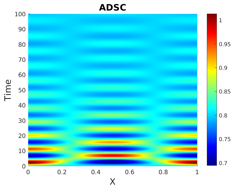
c1(x,0)=c1,c2(x,0)=c2+0.1exp((x.5)2/0.2),h(x,0)=h,b=3.7(b=1.8).formulae-sequencesubscript𝑐1𝑥0superscriptsubscript𝑐1formulae-sequencesubscript𝑐2𝑥0superscriptsubscript𝑐20.1superscript𝑥.520.2formulae-sequence𝑥0superscript𝑏3.7𝑏1.8\displaystyle c_{1}(x,0)=c_{1}^{*},\ c_{2}(x,0)=c_{2}^{*}+0.1\exp(-(x-.5)^{2}/0.2),\ h(x,0)=h^{*},\ b=3.7\ (b=1.8).
Refer to caption
(a) ADSCs for b=3.7𝑏3.7b=3.7
Refer to caption
(b) Chondrocytes for b=3.7𝑏3.7b=3.7
Refer to caption
(c) Hyaluron & ECM for b=3.7𝑏3.7b=3.7
Refer to caption
(d) ADSCs for b=1.8𝑏1.8b=1.8
Refer to caption
(e) Chondrocytes for b=1.8𝑏1.8b=1.8
Refer to caption
(f) Hyaluron & ECM for b=1.8𝑏1.8b=1.8
Figure 1: ADSC, chondrocyte, and hyaluron/ECM density for Scenario 1. Upper row: b>bc𝑏subscript𝑏𝑐b>b_{c}, lower row b<bc𝑏subscript𝑏𝑐b<b_{c}.

Figure 1 shows the simulated patterns for Scenario 1 when the tactic sensitivity coefficient b𝑏b exceeds the critical bifurcation value bcsubscript𝑏𝑐b_{c} (upper row of plots) and when it is below it (lower row). The former situation leads as expected to oscillatory behavior of all three solution components, accentuated for ADSC and chondrocytes, which infer motility. The oscillations are very slowly damped, mainly due to the cells diffusing and spreading within the whole simulated domain. When b>bc𝑏subscript𝑏𝑐b>b_{c} the incipient perturbation of the system’s steady state is quickly losing its effect, which is in line with the result in Proposition 1.

Using as initial condition the same perturbation of steady-states, but applying it to different components of the solution leads to changes in the overall behavior of the system, as Figures 2 and 3 produced by Scenarios 2 and 3 are showing, respectively. The former includes a perturbation of ADSC density and Figure 2 exhibits a behavior similar to that in Figure 1, with the difference that the solution is stabilizing faster and at lower densities. Scenario 3 features the same perturbation, but of hyaluron and ECM, i.e. of the tactic signal. The effect is substantial: the oscillations are far weaker, even for b>bc𝑏subscript𝑏𝑐b>b_{c} and damped rapidly, while higher densities of ADSCs, chondrocytes, and hylauron/ECM are obtained. This seems to be the most favorable case for the envisaged tissue regeneration.

Scenario 2: x[0,1]𝑥01x\in[0,1], perturbed initial amount of ADSCs:
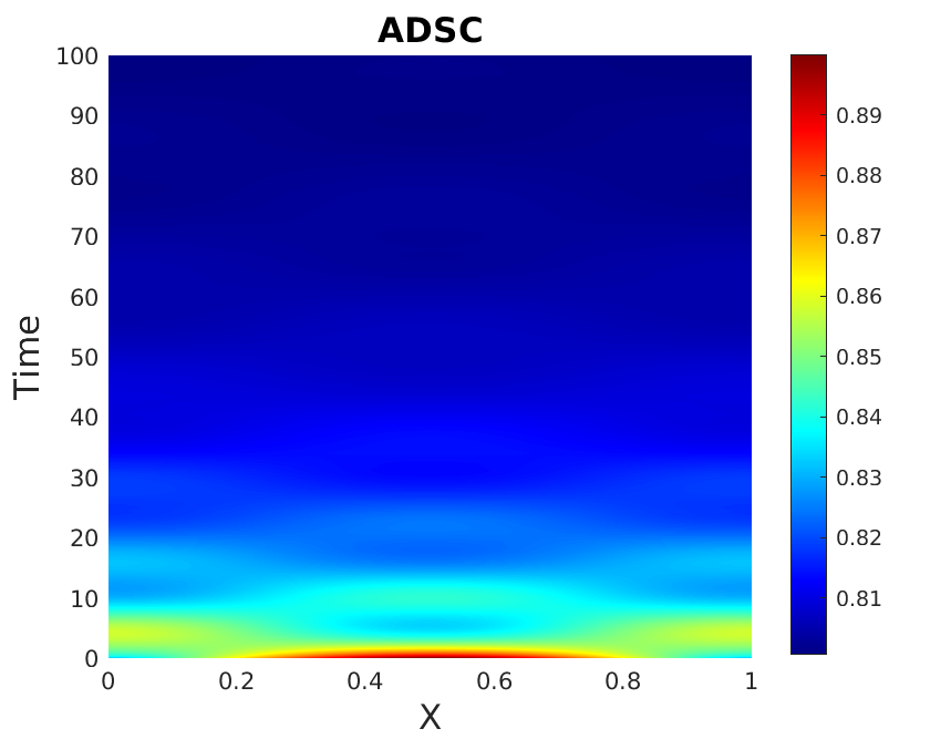
c1(x,0)=c1+0.1exp((x.5)2/0.2),c2(x,0)=c2,h(x,0)=h,b=3.7(b=1.8).formulae-sequencesubscript𝑐1𝑥0superscriptsubscript𝑐10.1superscript𝑥.520.2formulae-sequencesubscript𝑐2𝑥0superscriptsubscript𝑐2formulae-sequence𝑥0superscript𝑏3.7𝑏1.8\displaystyle c_{1}(x,0)=c_{1}^{*}+0.1\exp(-(x-.5)^{2}/0.2),\ c_{2}(x,0)=c_{2}^{*},\ h(x,0)=h^{*},\ b=3.7\ (b=1.8).
Refer to caption
(a) ADSCs for b=3.7𝑏3.7b=3.7
Refer to caption
(b) Chondrocytes for b=3.7𝑏3.7b=3.7
Refer to caption
(c) Hyaluron & ECM for b=3.7𝑏3.7b=3.7
Refer to caption
(d) ADSCs for b=1.8𝑏1.8b=1.8
Refer to caption
(e) Chondrocytes for b=1.8𝑏1.8b=1.8
Refer to caption
(f) Hyaluron & ECM for b=1.8𝑏1.8b=1.8
Figure 2: ADSC, chondrocyte, and hyaluron/ECM density for Scenario 2. Upper row: b>bc𝑏subscript𝑏𝑐b>b_{c}, lower row b<bc𝑏subscript𝑏𝑐b<b_{c}.

Scenario 3: x[0,1]𝑥01x\in[0,1], perturbed initial amount of hyaluron & ECM:
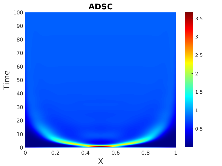
c1(x,0)=c1,c2(x,0)=c2,h(x,0)=h+0.1exp((x.5)2/0.2),b=3.7.formulae-sequencesubscript𝑐1𝑥0superscriptsubscript𝑐1formulae-sequencesubscript𝑐2𝑥0superscriptsubscript𝑐2formulae-sequence𝑥0superscript0.1superscript𝑥.520.2𝑏3.7\displaystyle c_{1}(x,0)=c_{1}^{*},\ c_{2}(x,0)=c_{2}^{*},\ h(x,0)=h^{*}+0.1\exp(-(x-.5)^{2}/0.2),\ b=3.7.
Refer to caption
(a) ADSCs for b=3.7𝑏3.7b=3.7
Refer to caption
(b) Chondrocytes for b=3.7𝑏3.7b=3.7
Refer to caption
(c) Hyaluron & ECM for b=3.7𝑏3.7b=3.7
Figure 3: ADSC, chondrocyte, and hyaluron/ECM density for Scenario 3, b>bc𝑏subscript𝑏𝑐b>b_{c}.

In the following Scenario 4 we consider initial periodic perturbations of the ADSC and hyaluron/ECM steady-states and enlarge the simulation domain ten times. The simulation results are shown in Figure 4. The periodic patterns are somewhat reminiscent to the used perturbation with cosines, but only occur in this pregnance when the domain is large enough. The alternation of large and lower densities in the solution components is due to ADSCs performing taxis towards gradients of hh, whose dynamics is almost entirely controled by chondrocytes. As in the previous figures, a small enough tactic sensitivity b<bc𝑏subscript𝑏𝑐b<b_{c} leads to quicker stabilization to lower densities of cells (of both phenotypes) and tissue.

Scenario 4: x[0,10]𝑥010x\in[0,10], perturbed initial amounts of ADSC and hyaluron & ECM:
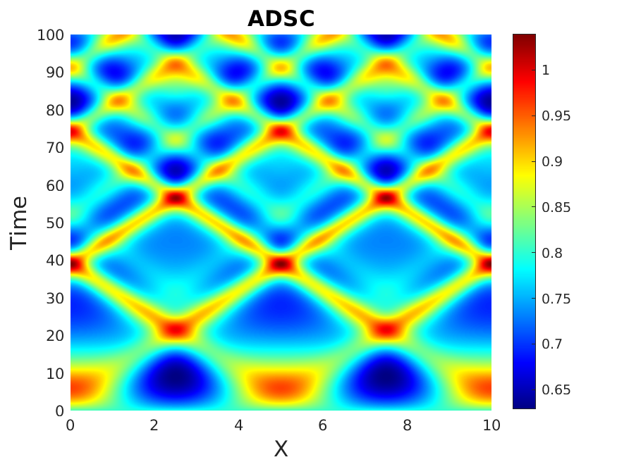
c1(x,0)=c1+.01cos(4π(x5)/10),c2(x,0)=c2,h(x,0)=h+.01cos(4π(x5)/10),formulae-sequencesubscript𝑐1𝑥0superscriptsubscript𝑐1.014𝜋𝑥510formulae-sequencesubscript𝑐2𝑥0superscriptsubscript𝑐2𝑥0superscript.014𝜋𝑥510\displaystyle c_{1}(x,0)=c_{1}^{*}+.01\cos(4\pi(x-5)/10),\ c_{2}(x,0)=c_{2}^{*},\ h(x,0)=h^{*}+.01\cos(4\pi(x-5)/10),
b=3.7(b=1.8).𝑏3.7𝑏1.8\displaystyle b=3.7\ (b=1.8).
Refer to caption
(a) ADSCs for b=3.7𝑏3.7b=3.7
Refer to caption
(b) Chondrocytes for b=3.7𝑏3.7b=3.7
Refer to caption
(c) Hyaluron & ECM for b=3.7𝑏3.7b=3.7
Refer to caption
(d) ADSCs for b=1.8𝑏1.8b=1.8
Refer to caption
(e) Chondrocytes for b=1.8𝑏1.8b=1.8
Refer to caption
(f) Hyaluron & ECM for b=1.8𝑏1.8b=1.8
Figure 4: ADSC, chondrocyte, and hyaluron/ECM density for Scenario 4. Upper row: b>bc𝑏subscript𝑏𝑐b>b_{c}, lower row b<bc𝑏subscript𝑏𝑐b<b_{c}.

4.2 2D simulations

The 2D discretization of the model is done using the finite difference method (FDM). A standard central difference scheme is used to discretize the diffusion parts of the equations for ADSCs and chondrocytes, while the taxis term in the ADSC equation was handled by a first order upwind scheme. For the time derivatives an implicit-explicit (IMEX) scheme is used, thereby treating the diffusion parts implicitly and discretizing the taxis and source terms with an explicit Euler method.

The initial conditions considered in this case are

c1(x,0)=c1+106exp(((x5)2+(y5)2)/.2),subscript𝑐1𝑥0superscriptsubscript𝑐1superscript106superscript𝑥52superscript𝑦52.2\displaystyle c_{1}(x,0)=c_{1}^{*}+10^{-6}\exp(-((x-5)^{2}+(y-5)^{2})/.2),
c2(x,0)=c2+109exp(((x5)2+(y5)2)/.2),h(x,0)=1+106U,formulae-sequencesubscript𝑐2𝑥0superscriptsubscript𝑐2superscript109superscript𝑥52superscript𝑦52.2𝑥01superscript106𝑈\displaystyle c_{2}(x,0)=c_{2}^{*}+10^{-9}\exp(-((x-5)^{2}+(y-5)^{2})/.2),\ h(x,0)=1+10^{-6}U, (4.1)

where U𝑈U represents a uniform distribution within (0,1)01(0,1). Figure 5 shows their plots.
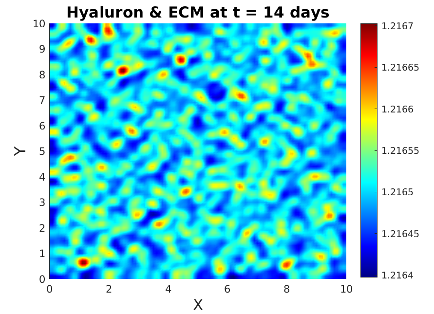
Refer to caption
Refer to caption
Refer to caption
Figure 5: Initial conditions (4.2) for ADSC, chondrocyte, and hyaluron/ECM density.
Refer to caption
(a) ADSCs at 7 days
Refer to caption
(b) ADSCs at 14 days
Refer to caption
(c) ADSCs at 21 days
Refer to caption
(d) Chondrocytes at 7 days
Refer to caption
(e) Chondrocytes at 14 days
Refer to caption
(f) Chondrocytes at 14 days
Refer to caption
(g) Hyaluron & ECM at 7 days
Refer to caption
(h) Hyaluron & ECM at 14 days
Refer to caption
(i) Hyaluron & ECM at 21 days
Figure 6: ADSC, chondrocyte, and hyaluron/ECM density at 7, 14, and 21 days, initial conditions (4.2), b>bc𝑏subscript𝑏𝑐b>b_{c} (here b=3.7𝑏3.7b=3.7)

Figure 6 illustrates the 2D simulation results for system (3.1) under conditions (4.2). Densities of ADSCs, chondrocytes, and hyaluron/ECM are shown at 7, 14, and 21 days. The tactic sensitivity parameter b=3.7𝑏3.7b=3.7 exceeds the threshold obtained in Section 3.2 as Hopf bifurcation value. The cells are quickly diffusing from the initial positions. The motility of ADSCs is further enhanced by taxis towards gradients of signal hh and the chondrocytes follow, as they are only obtained by ADSC differentiation. This behavior can also be observed in Figure 7, which shows the same evolution of c1,c2,hsubscript𝑐1subscript𝑐2c_{1},\ c_{2},\ h, but for b=1.8<bc𝑏1.8subscript𝑏𝑐b=1.8<b_{c}. A higher tactic sensitivity of ADSCs seems to lead as in the 1D case to slightly increased densities of cells and tissue.
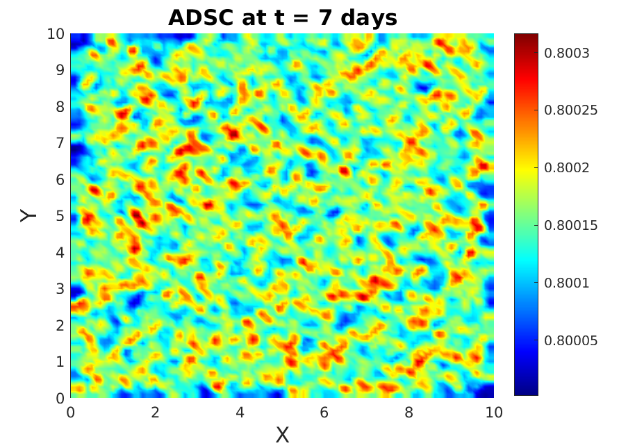
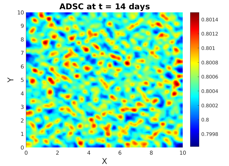
Refer to caption
(a) ADSCs at 7 days
Refer to caption
(b) ADSCs at 14 days
Refer to caption
(c) ADSCs at 21 days
Refer to caption
(d) Chondrocytes at 7 days
Refer to caption
(e) Chondrocytes at 14 days
Refer to caption
(f) Chondrocytes at 14 days
Refer to caption
(g) Hyaluron & ECM at 7 days
Refer to caption
(h) Hyaluron & ECM at 14 days
Refer to caption
(i) Hyaluron & ECM at 21 days
Figure 7: ADSC, chondrocyte, and hyaluron/ECM density at 7, 14, and 21 days, initial conditions (4.2), b<bc𝑏subscript𝑏𝑐b<b_{c} (here b=1.8𝑏1.8b=1.8)

To investigate the effect of initial hyaluron (and hence of tissue) distribution we considered

c1(x,0)=c1+106exp(((x5)2+(y5)2)/.2),subscript𝑐1𝑥0superscriptsubscript𝑐1superscript106superscript𝑥52superscript𝑦52.2\displaystyle c_{1}(x,0)=c_{1}^{*}+10^{-6}\exp(-((x-5)^{2}+(y-5)^{2})/.2), (4.2)
c2(x,0)=c2+109exp(((x5)2+(y5)2)/.2),h(x,0)=1+106Ucos(4π(x5)/10).formulae-sequencesubscript𝑐2𝑥0superscriptsubscript𝑐2superscript109superscript𝑥52superscript𝑦52.2𝑥01superscript106𝑈4𝜋𝑥510\displaystyle c_{2}(x,0)=c_{2}^{*}+10^{-9}\exp(-((x-5)^{2}+(y-5)^{2})/.2),\ h(x,0)=1+10^{-6}U\cos(4\pi(x-5)/10).

The corresponding simulation results are shown in Figure 9. The previously mentioned behavior of cells and tissue is more pregnantly visible: the cells leave the rather concentrated initial blob, the ADSCs follow the tissue signal and make the chondrocytes follow in turn. This allows for higher cell and tissue densities along the ’stripes’ generated by the cosine in (4.2), suggesting that the initial structure of underlying tissue plays a major role during the regeneration process. Thus, properly designed scaffolds providing support for cell migration can have a relevant influence on the amount and quality of newly produced tissue upon seeding with stem cells and promoting and sustaining differentiation into chondrocytes.

Refer to caption
Refer to caption
Refer to caption
Figure 8: Initial conditions (4.2) for ADSC, chondrocyte, and hyaluron/ECM density.
Refer to caption
(a) ADSCs at 7 days
Refer to caption
(b) ADSCs at 14 days
Refer to caption
(c) ADSCs at 21 days
Refer to caption
(d) Chondrocytes at 7 days
Refer to caption
(e) Chondrocytes at 14 days
Refer to caption
(f) Chondrocytes at 14 days
Refer to caption
(g) Hyaluron & ECM at 7 days
Refer to caption
(h) Hyaluron & ECM at 14 days
Refer to caption
(i) Hyaluron & ECM at 21 days
Figure 9: ADSC, chondrocyte, and hyaluron/ECM density at 7, 14, and 21 days, initial conditions (4.2), b>bc𝑏subscript𝑏𝑐b>b_{c} (here b=3.7𝑏3.7b=3.7)

Appendix A Appendix

The subsequent lemma closely follows Lemma A in the appendix of [31]:

Lemma A.1.

Assuming 0<T<10𝑇10<T<1, c2jC65,35(QT)subscript𝑐2𝑗superscript𝐶6535subscript𝑄𝑇c_{2j}\in C^{\frac{6}{5},\frac{3}{5}}(Q_{T}), c2j0subscript𝑐2𝑗0c_{2j}\geq 0, hjC(0,T;W1,5(Ω))subscript𝑗𝐶0𝑇superscript𝑊15Ωh_{j}\in C(0,T;W^{1,5}(\Omega)) and zjC1,0(Q¯T)(j=1,2)subscript𝑧𝑗superscript𝐶10subscript¯𝑄𝑇𝑗12z_{j}\in C^{1,0}(\bar{Q}_{T})(j=1,2) and zjC1,0(Q¯T)M,hjC(0,T;W1,5(Ω))Mformulae-sequencesubscriptnormsubscript𝑧𝑗superscript𝐶10subscript¯𝑄𝑇𝑀subscriptnormsubscript𝑗𝐶0𝑇superscript𝑊15Ω𝑀\|z_{j}\|_{C^{1,0}(\bar{Q}_{T})}\leq M,\|h_{j}\|_{C(0,T;W^{1,5}(\Omega))}\leq M and c2jC65,35(QT)Msubscriptnormsubscript𝑐2𝑗superscript𝐶6535subscript𝑄𝑇𝑀\|c_{2j}\|_{C^{\frac{6}{5},\frac{3}{5}}(Q_{T})}\leq M. Then the solutions h¯1subscript¯1\bar{h}_{1} and h¯2subscript¯2\bar{h}_{2} of the ordinary differential equations

th¯j=γ1h¯jc2j+γ2c2jKc2+c2j,hj(x,0)=h0(x),j=1,2formulae-sequencesubscript𝑡subscript¯𝑗subscript𝛾1subscript¯𝑗subscript𝑐2𝑗subscript𝛾2subscript𝑐2𝑗subscript𝐾subscript𝑐2subscript𝑐2𝑗formulae-sequencesubscript𝑗𝑥0subscript0𝑥𝑗12\partial_{t}\bar{h}_{j}=-\gamma_{1}\bar{h}_{j}c_{2j}+\gamma_{2}\frac{c_{2j}}{K_{c_{2}}+c_{2j}},\quad h_{j}(x,0)=h_{0}(x),\quad j=1,2 (A.1)

satisfy

h¯1h¯2C(0,T;W1,5(Ω))TC(M)((c21c22)C1,0(QT)+z1z2C1,0(QT)+h1h2C(0,T;W1,5(Ω))),subscriptnormsubscript¯1subscript¯2𝐶0𝑇superscript𝑊15Ω𝑇𝐶𝑀subscriptnormsubscript𝑐21subscript𝑐22superscript𝐶10subscript𝑄𝑇subscriptnormsubscript𝑧1subscript𝑧2superscript𝐶10subscript𝑄𝑇subscriptnormsubscript1subscript2𝐶0𝑇superscript𝑊15Ω\|\bar{h}_{1}-\bar{h}_{2}\|_{C(0,T;W^{1,5}(\Omega))}\leq TC(M)(\|(c_{21}-c_{22})\|_{C^{1,0}(Q_{T})}+\|z_{1}-z_{2}\|_{C^{1,0}(Q_{T})}+\|h_{1}-h_{2}\|_{C(0,T;W^{1,5}(\Omega))}), (A.2)

where C(M)𝐶𝑀C(M) is a constant depending only on M𝑀M.

Proof.

We can directly have the following ODE from (A.1)

t(h¯1h¯2)=w1(h¯1h¯2)+w2,h¯1(x,0)h¯2(x,0)=0formulae-sequencesubscript𝑡subscript¯1subscript¯2subscript𝑤1subscript¯1subscript¯2subscript𝑤2subscript¯1𝑥0subscript¯2𝑥00\partial_{t}(\bar{h}_{1}-\bar{h}_{2})=w_{1}(\bar{h}_{1}-\bar{h}_{2})+w_{2},\quad\bar{h}_{1}(x,0)-\bar{h}_{2}(x,0)=0 (A.3)

where w1=γ1c21,w2=(c21c22){γ1h¯2+γ2Kc1(Kc1+c21)(Kc1+c22)}formulae-sequencesubscript𝑤1subscript𝛾1subscript𝑐21subscript𝑤2subscript𝑐21subscript𝑐22subscript𝛾1subscript¯2subscript𝛾2subscript𝐾subscript𝑐1subscript𝐾subscript𝑐1subscript𝑐21subscript𝐾subscript𝑐1subscript𝑐22w_{1}=-\gamma_{1}c_{21},\leavevmode\nobreak\ w_{2}=(c_{21}-c_{22})\left\{-\gamma_{1}\bar{h}_{2}+\frac{\gamma_{2}K_{c_{1}}}{(K_{c_{1}}+c_{21})(K_{c_{1}}+c_{22})}\right\}. Solving (A.3)

(h¯1h¯2)(x,t)=0testw1(x,τ)𝑑τw2(x,s)𝑑ssubscript¯1subscript¯2𝑥𝑡superscriptsubscript0𝑡superscript𝑒superscriptsubscript𝑠𝑡subscript𝑤1𝑥𝜏differential-d𝜏subscript𝑤2𝑥𝑠differential-d𝑠(\bar{h}_{1}-\bar{h}_{2})(x,t)=\int_{0}^{t}e^{\int_{s}^{t}w_{1}(x,\tau)d\tau}w_{2}(x,s)ds

and

(h¯1h¯2)(x,t)=0testw1(x,τ)𝑑τw2(x,s)𝑑s+0testw1(x,τ)𝑑τw2(x,s)stw1(x,τ)𝑑τ𝑑s.subscript¯1subscript¯2𝑥𝑡superscriptsubscript0𝑡superscript𝑒superscriptsubscript𝑠𝑡subscript𝑤1𝑥𝜏differential-d𝜏subscript𝑤2𝑥𝑠differential-d𝑠superscriptsubscript0𝑡superscript𝑒superscriptsubscript𝑠𝑡subscript𝑤1𝑥𝜏differential-d𝜏subscript𝑤2𝑥𝑠superscriptsubscript𝑠𝑡subscript𝑤1𝑥𝜏differential-d𝜏differential-d𝑠(\nabla\bar{h}_{1}-\nabla\bar{h}_{2})(x,t)=\int_{0}^{t}e^{\int_{s}^{t}w_{1}(x,\tau)d\tau}\nabla w_{2}(x,s)ds+\int_{0}^{t}e^{\int_{s}^{t}w_{1}(x,\tau)d\tau}w_{2}(x,s)\int_{s}^{t}\nabla w_{1}(x,\tau)d\tau ds.

We can find a C(M)𝐶𝑀C(M) such that, w1C(QT)C(M)subscriptnormsubscript𝑤1𝐶subscript𝑄𝑇𝐶𝑀\|w_{1}\|_{C(Q_{T})}\leq C(M), also

w1C(0,T;L5(Ω))=γ1c21C(0,T;L5(Ω))C(M),subscriptnormsubscript𝑤1𝐶0𝑇superscript𝐿5Ωsubscript𝛾1subscriptnormsubscript𝑐21𝐶0𝑇superscript𝐿5Ω𝐶𝑀\displaystyle\|\nabla w_{1}\|_{C(0,T;L^{5}(\Omega))}=\gamma_{1}\|\nabla c_{21}\|_{C(0,T;L^{5}(\Omega))}\leq C(M),
w2C(QT)subscriptnormsubscript𝑤2𝐶subscript𝑄𝑇\displaystyle\|w_{2}\|_{C(Q_{T})} =γ1h¯2(c21c22)+γ2Kc1(c21c22)(Kc1+c21)(Kc1+c22)C(QT)C(M)(c21c22)C(QT)absentsubscriptnormsubscript𝛾1subscript¯2subscript𝑐21subscript𝑐22subscript𝛾2subscript𝐾subscript𝑐1subscript𝑐21subscript𝑐22subscript𝐾subscript𝑐1subscript𝑐21subscript𝐾subscript𝑐1subscript𝑐22𝐶subscript𝑄𝑇𝐶𝑀subscriptnormsubscript𝑐21subscript𝑐22𝐶subscript𝑄𝑇\displaystyle=\left\|-\gamma_{1}\bar{h}_{2}(c_{21}-c_{22})+\tfrac{\gamma_{2}K_{c_{1}}(c_{21}-c_{22})}{(K_{c_{1}}+c_{21})(K_{c_{1}}+c_{22})}\right\|_{C(Q_{T})}\leq C(M)\|(c_{21}-c_{22})\|_{C(Q_{T})}
C(M)((c21c22)C(QT)+z1z2C(QT)+h1h2C(0,T;W1,5(Ω)))absent𝐶𝑀subscriptnormsubscript𝑐21subscript𝑐22𝐶subscript𝑄𝑇subscriptnormsubscript𝑧1subscript𝑧2𝐶subscript𝑄𝑇subscriptnormsubscript1subscript2𝐶0𝑇superscript𝑊15Ω\displaystyle\leq C(M)(\|(c_{21}-c_{22})\|_{C(Q_{T})}+\|z_{1}-z_{2}\|_{C(Q_{T})}+\|h_{1}-h_{2}\|_{C(0,T;W^{1,5}(\Omega))})

and

w2C(0,T;L5(Ω))=\displaystyle\|\nabla w_{2}\|_{C(0,T;L^{5}(\Omega))}=\Big{\|} γ1(c21c22)h¯2γ1h¯2(c21c22)+γ2Kc1(Kc1+c21)(Kc1+c22)(c21c22)subscript𝛾1subscript𝑐21subscript𝑐22subscript¯2subscript𝛾1subscript¯2subscript𝑐21subscript𝑐22subscript𝛾2subscript𝐾subscript𝑐1subscript𝐾subscript𝑐1subscript𝑐21subscript𝐾subscript𝑐1subscript𝑐22subscript𝑐21subscript𝑐22\displaystyle-\gamma_{1}(c_{21}-c_{22})\nabla\bar{h}_{2}-\gamma_{1}\bar{h}_{2}(\nabla c_{21}-\nabla c_{22})+\tfrac{\gamma_{2}K_{c_{1}}}{(K_{c_{1}}+c_{21})(K_{c_{1}}+c_{22})}(\nabla c_{21}-\nabla c_{22})
γ2Kc1(c21c22)(Kc1+c21)2(Kc1+c22)c21γ2Kc1(c21c22)(Kc1+c21)(Kc1+c22)2c22C(0,T;L5(Ω))subscript𝛾2subscript𝐾subscript𝑐1subscript𝑐21subscript𝑐22superscriptsubscript𝐾subscript𝑐1subscript𝑐212subscript𝐾subscript𝑐1subscript𝑐22subscript𝑐21evaluated-atsubscript𝛾2subscript𝐾subscript𝑐1subscript𝑐21subscript𝑐22subscript𝐾subscript𝑐1subscript𝑐21superscriptsubscript𝐾subscript𝑐1subscript𝑐222subscript𝑐22𝐶0𝑇superscript𝐿5Ω\displaystyle-\tfrac{\gamma_{2}K_{c_{1}}(c_{21}-c_{22})}{(K_{c_{1}}+c_{21})^{2}(K_{c_{1}}+c_{22})}\nabla c_{21}-\tfrac{\gamma_{2}K_{c_{1}}(c_{21}-c_{22})}{(K_{c_{1}}+c_{21})(K_{c_{1}}+c_{22})^{2}}\nabla c_{22}\Big{\|}_{C(0,T;L^{5}(\Omega))}
C(M)((c21c22)C1,0(QT)\displaystyle\leq C(M)(\|(c_{21}-c_{22})\|_{C^{1,0}(Q_{T})}
C(M)((c21c22)C1,0(QT)+z1z2C1,0(QT)+h1h2C(0,T;W1,5(Ω)))absent𝐶𝑀subscriptnormsubscript𝑐21subscript𝑐22superscript𝐶10subscript𝑄𝑇normsubscript𝑧1subscript𝑧2superscript𝐶10subscript𝑄𝑇subscriptnormsubscript1subscript2𝐶0𝑇superscript𝑊15Ω\displaystyle\leq C(M)(\|(c_{21}-c_{22})\|_{C^{1,0}(Q_{T})}+\|z_{1}-z_{2}\|{C^{1,0}(Q_{T})}+\|h_{1}-h_{2}\|_{C(0,T;W^{1,5}(\Omega))})

Now, as in [31], we can also have the following two estimates

h¯1(,t)h¯2(,t)L5(Ω)TC(M)((c21c22)C(QT)+z1z2C(QT)+h1h2C(0,T;W1,5(Ω)))subscriptnormsubscript¯1𝑡subscript¯2𝑡superscript𝐿5Ω𝑇𝐶𝑀subscriptnormsubscript𝑐21subscript𝑐22𝐶subscript𝑄𝑇subscriptnormsubscript𝑧1subscript𝑧2𝐶subscript𝑄𝑇subscriptnormsubscript1subscript2𝐶0𝑇superscript𝑊15Ω\displaystyle\|\bar{h}_{1}(\cdot,t)-\bar{h}_{2}(\cdot,t)\|_{L^{5}(\Omega)}\leq TC(M)(\|(c_{21}-c_{22})\|_{C(Q_{T})}+\|z_{1}-z_{2}\|_{C(Q_{T})}+\|h_{1}-h_{2}\|_{C(0,T;W^{1,5}(\Omega))})

and

h¯1(,t)h¯2(,t)L5(Ω)TC(M)((c21c22)C1,0(QT)\displaystyle\|\nabla\bar{h}_{1}(\cdot,t)-\nabla\bar{h}_{2}(\cdot,t)\|_{L^{5}(\Omega)}\leq TC(M)\big{(}\|(c_{21}-c_{22})\|_{C^{1,0}(Q_{T})} +z1z2C1,0(QT)subscriptnormsubscript𝑧1subscript𝑧2superscript𝐶10subscript𝑄𝑇\displaystyle+\|z_{1}-z_{2}\|_{C^{1,0}(Q_{T})}
+h1h2C(0,T;W1,5(Ω))).\displaystyle+\|h_{1}-h_{2}\|_{C(0,T;W^{1,5}(\Omega))}\big{)}.

Acknowledgement

CS and NM acknowledge funding by the German Research Foundation DFG within the SPP 2311. SCM was funded by DAAD, MathApp, and the Nachwuchsring at RPTU Kaiserslautern-Landau.

References

  • [1] H Amann “Hopf bifurcation in quasilinear reaction-diffusion systems” In S. Busenberg, M. Martelli (Eds.), Delay Differential Equations and Dynamical Systems, in: Lect. Notes Math. 1475 Springer, 1991, pp. 53–63
  • [2] Kyriacos A. Athanasiou and Johannah Sanchez-Adams “Engineering the Knee Meniscus” In Synthesis Lectures on Tissue Engineering Springer International Publishing, 2009 DOI: 10.1007/978-3-031-02576-1
  • [3] X Bai and M Winkler “Equilibration in a Fully Parabolic Two-Species Chemotaxis System with Competitive Kinetics” In Indiana University Mathematics Journal 65.2, 2016
  • [4] N. Bellomo “Modeling Complex Living Systems” Birkhäuser Boston, 2008 DOI: 10.1007/978-0-8176-4600-4
  • [5] Edoardo Borgiani, Georg N. Duda and Sara Checa “Multiscale Modeling of Bone Healing: Toward a Systems Biology Approach” In Frontiers in Physiology 8 Frontiers Media SA, 2017 DOI: 10.3389/fphys.2017.00287
  • [6] Martina Conte, Yvonne Dzierma, Sven Knobe and Christina Surulescu “Mathematical modeling of glioma invasion and therapy approaches via kinetic theory of active particles” In Mathematical Models and Methods in Applied Sciences World Scientific, 2023, pp. 1–43
  • [7] Martina Conte and Christina Surulescu “Mathematical modeling of glioma invasion: acid- and vasculature mediated go-or-grow dichotomy and the influence of tissue anisotropy” In Applied Mathematics and Computation 407 Elsevier BV, 2021, pp. 126305 DOI: 10.1016/j.amc.2021.126305
  • [8] Gregor Corbin et al. “Modeling glioma invasion with anisotropy-and hypoxia-triggered motility enhancement: From subcellular dynamics to macroscopic PDEs with multiple taxis” In Mathematical Models and Methods in Applied Sciences 31.01 World Scientific, 2021, pp. 177–222
  • [9] Anne Dietrich, Niklas Kolbe, Nikolaos Sfakianakis and Christina Surulescu “Multiscale modeling of glioma invasion: from receptor binding to flux-limited macroscopic PDEs” In Multiscale Modeling & Simulation 20.2 SIAM, 2022, pp. 685–713
  • [10] C. Engwer, T. Hillen, M. Knappitsch and C. Surulescu “Glioma follow white matter tracts: a multiscale DTI-based model” In Journal of Mathematical Biology 71.3 Springer ScienceBusiness Media LLC, 2014, pp. 551–582 DOI: 10.1007/s00285-014-0822-7
  • [11] Christian Engwer, Thomas Hillen, Markus Knappitsch and Christina Surulescu “Glioma follow white matter tracts: a multiscale DTI-based model” In Journal of mathematical biology 71 Springer, 2015, pp. 551–582
  • [12] Christian Engwer, Alexander Hunt and Christina Surulescu “Effective equations for anisotropic glioma spread with proliferation: a multiscale approach and comparisons with previous settings” In Mathematical medicine and biology: a journal of the IMA 33.4 Oxford University Press, 2016, pp. 435–459
  • [13] Jan Giesselmann, Niklas Kolbe and Nikolaos Sfakianakis “Existence and uniqueness of global classical solutions to a two dimensional two species cancer invasion haptotaxis model” In Discrete & Continuous Dynamical Systems-B 23.10 American Institute of Mathematical Sciences, 2018, pp. 4397
  • [14] E. Grosjean, B. Simeon and C. Surulescu “A mathematical model for meniscus cartilage regeneration” In PAMM 23.3 Wiley, 2023 DOI: 10.1002/pamm.202300261
  • [15] Elise Grosjean et al. “An in-silico approach to meniscus tissue regeneration: Modeling, numerical simulation, and experimental analysis” In preprint, 2024
  • [16] Weimin Guo et al. “Advances and Prospects in Tissue-Engineered Meniscal Scaffolds for Meniscus Regeneration” In Stem Cells International 2015 Hindawi Limited, 2015, pp. 1–13 DOI: 10.1155/2015/517520
  • [17] Alexander Hunt and Christina Surulescu “A Multiscale Modeling Approach to Glioma Invasion with Therapy” In Vietnam Journal of Mathematics 45.1-2 Springer ScienceBusiness Media LLC, 2016, pp. 221–240 DOI: 10.1007/s10013-016-0223-x
  • [18] B Johnstone et al. “Tissue engineering for articular cartilage repair – the state of the art” In European Cells and Materials 25 European CellsMaterials, 2013, pp. 248–267 DOI: 10.22203/ecm.v025a18
  • [19] Yuanyuan Ke and Jiashan Zheng “A note for global existence of a two-dimensional chemotaxis–haptotaxis model with remodeling of non-diffusible attractant” In Nonlinearity 31.10 IOP Publishing, 2018, pp. 4602
  • [20] Pawan Kumar, Jing Li and Christina Surulescu “Multiscale modeling of glioma pseudopalisades: contributions from the tumor microenvironment” In Journal of Mathematical Biology 82 Springer, 2021, pp. 1–45
  • [21] OA Ladyzenskaja, VA Solonnikov and NN Ural’Ceva “Linear aad quaslinear equations of parabolic type” In Trans. Math. Monographs, Am. Soc, Provindence RI 23, 1968
  • [22] Ping Liu, Junping Shi and Zhi-An Wang “Pattern formation of the attraction-repulsion Keller-Segel system” In Discrete & Continuous Dynamical Systems-B 18.10 American Institute of Mathematical Sciences, 2013, pp. 2597
  • [23] MC Lombardo et al. “Demyelination patterns in a mathematical model of multiple sclerosis” In Journal of mathematical biology 75.2 Springer, 2017, pp. 373–417
  • [24] N. Loy and L. Preziosi “Kinetic models with non-local sensing determining cell polarization and speed according to independent cues” In Journal of Mathematical Biology Springer, 2019, pp. 1–49
  • [25] Anna Marciniak-Czochra and Mariya Ptashnyk “Boundedness of solutions of a haptotaxis model” In Mathematical Models and Methods in Applied Sciences 20.03 World Scientific, 2010, pp. 449–476
  • [26] P Mishra and D Wrzosek “Indirect taxis drives spatio-temporal patterns in an extended Schoener’s intraguild predator–prey model” In Applied Mathematics Letters Elsevier, 2022
  • [27] P Mishra and D Wrzosek “Repulsive chemotaxis and predator evasion in predator prey models with diffusion and prey taxis” In Math. Models Methods Appl. Sci. 32, 2022, pp. 1–42
  • [28] Giuseppe Orlando et al. “Regenerative Medicine as Applied to General Surgery” In Annals of Surgery 255.5 Ovid Technologies (Wolters Kluwer Health), 2012, pp. 867–880 DOI: 10.1097/sla.0b013e318243a4db
  • [29] K Osaki, T Tsujikawa, A Yagi and M Mimura “Exponential attractor for a chemotaxis growth system of equations” In Nonlinear Anal., 51, 2002, pp. 119–144
  • [30] H.G. Othmer and T. Hillen “The Diffusion Limit of Transport Equations II: Chemotaxis Equations” In SIAM Journal on Applied Mathematics 62.4 Society for Industrial & Applied Mathematics (SIAM), 2002, pp. 1222–1250 DOI: 10.1137/s0036139900382772
  • [31] Peter YH Pang and Yifu Wang “Global existence of a two-dimensional chemotaxis–haptotaxis model with remodeling of non-diffusible attractant” In Journal of Differential Equations 263.2 Elsevier, 2017, pp. 1269–1292
  • [32] Mamatha M. Pillai, J. Gopinathan, R. Selvakumar and Amitava Bhattacharyya “Human Knee Meniscus Regeneration Strategies: a Review on Recent Advances” In Current Osteoporosis Reports 16.3 Springer ScienceBusiness Media LLC, 2018, pp. 224–235 DOI: 10.1007/s11914-018-0436-x
  • [33] Ramón G. Plaza “Derivation of a bacterial nutrient-taxis system with doubly degenerate cross-diffusion as the parabolic limit of a velocity-jump process” In Journal of Mathematical Biology 78.6 Springer ScienceBusiness Media LLC, 2019, pp. 1681–1711 DOI: 10.1007/s00285-018-1323-x
  • [34] Christian Stinner, Christina Surulescu and Michael Winkler “Global weak solutions in a PDE-ODE system modeling multiscale cancer cell invasion” In SIAM Journal on Mathematical Analysis 46.3 SIAM, 2014, pp. 1969–2007
  • [35] Christina Surulescu and Michael Winkler “Does indirectness of signal production reduce the explosion-supporting potential in chemotaxis–haptotaxis systems? Global classical solvability in a class of models for cancer invasion (and more)” In European Journal of Applied Mathematics 32.4 Cambridge University Press, 2021, pp. 618–651
  • [36] Y Tao and M Winkler “Large time Behavior in a Multidimensional Chemotaxis - Haptotaxis Model with Slow Signal Diffusion” In SIAM J. MATH. ANAL. 47.6, 2015, pp. 4229–4250
  • [37] Youshan Tao “Global existence for a haptotaxis model of cancer invasion with tissue remodeling” In Nonlinear Analysis: Real World Applications 12.1 Elsevier, 2011, pp. 418–435
  • [38] Youshan Tao “Global existence of classical solutions to a combined chemotaxis–haptotaxis model with logistic source” In Journal of Mathematical Analysis and applications 354.1 Elsevier, 2009, pp. 60–69
  • [39] Youshan Tao and Michael Winkler “Energy-type estimates and global solvability in a two-dimensional chemotaxis–haptotaxis model with remodeling of non-diffusible attractant” In Journal of Differential Equations 257.3 Elsevier, 2014, pp. 784–815
  • [40] Chinedu C. Ude et al. “Cartilage Regeneration by Chondrogenic Induced Adult Stem Cells in Osteoarthritic Sheep Model” In PLoS ONE 9.6 Public Library of Science (PLoS), 2014, pp. e98770 DOI: 10.1371/journal.pone.0098770
  • [41] K Wang, Q Wang and F Yu “Stationary and time-periodic patterns of two-predator and one-prey systems with prey-taxis” In Discrete and Continuous Dynamical Systems. 37, 2017, pp. 505–543
  • [42] Q Wang, J Yang and L Zhang “Time-periodic and stable patterns of a two- competing-species Keller-Segel chemotaxis model: Effect of cellular growth” In Discrete and Continuous Dynamical Systems. 22.9, 2017, pp. 3547–3574
  • [43] S. L. Waters, L. J. Schumacher and A. J. El Haj “Regenerative medicine meets mathematical modelling: developing symbiotic relationships” In npj Regenerative Medicine 6.1 Springer ScienceBusiness Media LLC, 2021 DOI: 10.1038/s41536-021-00134-2
  • [44] Michael Winkler “Aggregation vs. global diffusive behavior in the higher-dimensional Keller–Segel model” In Journal of Differential Equations 248.12 Elsevier, 2010, pp. 2889–2905
  • [45] Hana Yu, Adetola B Adesida and Nadr M Jomha “Meniscus repair using mesenchymal stem cells – a comprehensive review” In Stem Cell Research & Therapy 6.1 Springer ScienceBusiness Media LLC, 2015 DOI: 10.1186/s13287-015-0077-2
  • [46] Johannes Zellner et al. “Role of mesenchymal stem cells in tissue engineering of meniscus” In Journal of Biomedical Materials Research Part A 94A.4 Wiley, 2010, pp. 1150–1161 DOI: 10.1002/jbm.a.32796
  • [47] Hala Zreiqat, Colin R. Dunstan and Vicki (eds. Rosen “A Tissue Regeneration Approach to Bone and Cartilage Repair” In Mechanical Engineering Series Springer International Publishing, 2015 DOI: 10.1007/978-3-319-13266-2