Scalable approximation and solvers for ionic electrodiffusion in cellular geometries

Abstract

The activity and dynamics of excitable cells are fundamentally regulated and moderated by extracellular and intracellular ion concentrations and their electric potentials. The increasing availability of dense reconstructions of excitable tissue at extreme geometric detail pose a new and clear scientific computing challenge for computational modelling of ion dynamics and transport. In this paper, we design, develop and evaluate a scalable numerical algorithm for solving the time-dependent and nonlinear KNP-EMI equations describing ionic electrodiffusion for excitable cells with an explicit geometric representation of intracellular and extracellular compartments and interior interfaces. We also introduce and specify a set of model scenarios of increasing complexity suitable for benchmarking. Our solution strategy is based on an implicit-explicit discretization and linearization in time, a mixed finite element discretization of ion concentrations and electric potentials in intracellular and extracellular domains, and an algebraic multigrid-based, inexact block-diagonal preconditioner for GMRES. Numerical experiments with up to $10^{8}$ unknowns per time step and up to 256 cores demonstrate that this solution strategy is robust and scalable with respect to the problem size, time discretization and number of cores.

65F10, 65N30, 65N55, 68U20, 68W10, 92-08, 92C20

1 Introduction

Our brains are composed of intertangled tissue consisting of neurons, glial cells and interstitial space, penetrated by blood vessels. Ions, such as potassium (K⁺), sodium (Na⁺), calcium (Ca²⁺) and chloride (Cl^-), move within and between the intracellular and extracellular compartments in a highly regulated manner. These ions, their movement and concentration differences, are fundamental for the function and well-being of the brain [52, 45]. For instance, the brain’s electrical signals fundamentally rely on action potentials induced by rapid neuronal influx of Na⁺ and efflux of K⁺ [52]. Moreover, ion concentrations and importantly ion concentration gradients may modulate brain signalling, regulate brain volume, and control brain states [41, 4, 45]. Notably, these physiological processes are only partially understood and currently attract substantial interest from the neurosciences [35, 45, 60, 6, 56, 43, 20]. High-fidelity in-silico studies would offer an innovative avenue of investigation with significant scientific potential.

Electrical and chemical activity in excitable tissue are naturally modelled via coupled partial differential equations (PDEs) describing ionic electrodiffusion [39, 42, 38, 21, 22]. These models go beyond the classical electrophysiology models, such as the monodomain or bidomain equations [53] and their cellular-level counterparts [3, 54], by describing spatial and temporal variations of ion concentrations in addition to the electric potentials. Within this context, we here consider explicit geometric representations of the intracellular and extracellular compartments and their joint interface representing the cell membrane [39, 61, 22]; i.e., the so-called KNP-EMI model (Kirchhoff-Nernst-Planck, extracellular-membrane-intracellular). In their seminal research [39], Mori and Peskin introduced and analyzed a finite volume-based spatial discretization of these cell-based ionic electrodiffusion equations, with numerical experiments in idealized two- and three-dimensional geometries. Similar equations and approximation challenges are also encountered in connection with ionic transport in lithium-ion batteries [32]. In our previous work [22], we introduced a mixed-dimensional mortar finite element method for these equations, again with numerical experiments limited to idealized geometries, and with little attention to computational performance.

Dense reconstructions and segmentations of brain tissue are increasingly becoming openly available [40, 62, 17, 36]. These imaging-based representations reveal an extraordinary geometric complexity that is very different from the more structured layers of cardiac tissue [14, 30]. This complexity places clear demands on the scalability of numerical solution algorithms. Solvers for the EMI (or cell-by-cell) electrophysiology equations, which can be viewed as a subsystem of the ionic electrodiffusion equations, have been studied quite intensively in recent years [3, 54, 11], including finite difference based methods [31], mixed finite element methods with and without Lagrange multipliers [54], boundary element methods [46], cut finite element methods [13], and finite volume methods [58]. Another key topic is scalable preconditioning [29, 11], and we highlight the scalable solution strategy for electrodiffusion (without interior interfaces) using a discontinuous Galerkin discretization proposed by Roy et al [47]. Parallel scalability may also be approached via domain decomposition techniques [29, 31], though the transition to complex geometries pose additional challenges. In fact, most studies consider highly idealized settings [39, 22], structured cell patterns as encountered in cardiac excitable tissue [54, 30], or simplified neuronal geometries [57, 59, 50, 15, 13, 24].

In this paper, we address the challenge of how to design scalable solution algorithms for the cell-based ionic electrodiffusion (KNP-EMI) equations with high geometric complexity and physiological membrane mechanisms. To this end, we present a lightweight single-dimensional finite element formulation with a scalable and efficient monolithic preconditioning strategy, vetted by a series of numerical experiments with realistic model parameters and geometries. The approximation scheme and solution strategy yield accurate solutions in a bounded (low) number of Krylov iterations. Near-optimal parallel scalability allows for rapidly obtaining solutions to large KNP-EMI problems using high performance computing systems, thus bridging the technology gap between dense tissue reconstructions and ionic electrodiffusion simulations.

This manuscript is organized as follows. In Section 2, we present the KNP-EMI equations and describe active and passive membrane dynamics involved in the interface coupling. In Section 3, we introduce a weak formulation of the continuous problem together with discretizations in time and space. In Section 4, we examine the block-structure and properties of the resulting discrete systems, and present a tailored solution strategy. In Section 5 we present four model scenarios in idealized and image-based geometries of increasing complexity defining a benchmark suite for KNP-EMI solvers. Section 6 reports on numerical experiments for the four scenarios, investigating robustness, efficiency, and parallel performance of the proposed strategy. Finally, Section 7 provides some concluding remarks and outlook.

2 A model for ionic electrodiffusion in cellular spaces

Following [22], we consider the domain $\Omega=\Omega_{i}\cup\Omega_{e}\cup\Gamma\subset\mathbb{R}^{d}$ for $d\in\{2,3\}$ with $\Omega_{i}$ and $\Omega_{e}$ representing the intra- and extracellular domains (ICS, ECS), respectively, and $\Gamma=\partial\Omega_{i}$ the cellular membrane(s). In general, the intracellular domain can be composed of $N_{\rm cell}\in\mathbb{N}$ disjoint domains $\Omega_{i}=\bigcup_{j=1}^{N_{\rm cell}}\Omega_{i,j}$, with $\Omega_{i,j}$ representing the $j$th (biological) cell with membrane $\Gamma_{j}=\partial\Omega_{i,j}$. We consider a set $K$ of ionic species, for example $K=\{\text{Na}^{+},\text{K}^{+},\text{Cl}^{-}\}$, with cardinality $|K|$. For each ionic species $k\in K$ and physical region $r\in\{i,e\}$, we model the evolution of ionic concentrations $[k]_{r}:\overline{\Omega}_{r}\times[0,T]\to\mathbb{R}$, as well as electric potentials $\phi_{r}:\overline{\Omega}_{r}\times[0,T]\to\mathbb{R}$.

2.1 Conservation equations

The assumption of conservation of ions for each region $r\in\{i,e\}$ yields the following time-dependent partial differential equation for each ionic species $k\in K$ and for $t\in(0,T)$ and $\bm{x}\in\Omega_{r}$:

(1) $$\partial_{t}[k]_{r}(\bm{x},t)+\nabla\cdot\mathbf{J}_{r}^{k}(\bm{x},t)=f_{r}^{k}(\bm{x},t),$$

where $\mathbf{J}_{r}^{k}:\overline{\Omega}_{r}\times[0,T]\to\mathbb{R}^{d}$ is the ion flux density. We consider a Nernst–Planck relation describing diffusion and drift in the electric field induced by the potential $\phi_{r}$:

(2) $$\mathbf{J}_{r}^{k}=\mathbf{J}_{r,\mathrm{diff}}^{k}+\mathbf{J}_{r,\mathrm{drift}}^{k}\\ =-D_{r}^{k}\nabla[k]_{r}-\frac{D_{r}^{k}z_{k}}{\psi}[k]_{r}\nabla\phi_{r},$$

where $D_{r}^{k}\in\mathbb{R}_{+}$ is the effective diffusion coefficient of ionic species $k$ in region $r$, $z_{k}$ is the valence of ion $k$, and $\psi=RTF^{-1}$ is composed of the gas constant $R$, the absolute temperature $T$, and the Faraday constant $F$. Finally, $f_{r}^{k}:\Omega_{r}\times[0,T]\to\mathbb{R}$ represent source terms. For consistency with the Kirchhoff-Nernst-Planck (KNP) assumption below, $f_{r}^{k}$ should maintain electroneutrality in the sense that

$$\sum_{k\in K}z_{k}f_{r}^{k}(\bm{x},t)=0\quad\text{ for }r\in\{i,e\}.$$

Equation (1) can be interpreted as an advection-diffusion equation with advection velocity given by the electric field $\nabla\phi_{r}$. Since $\phi_{r}$ is itself an unknown, it is not trivial to classify (1) as a diffusion- or advection-dominated problem a-priori. We note that (1) ignores convective effects due to movement of the domain or medium; thus assuming a medium at rest (see e.g. [21, 49] for contrast).

We introduce the KNP assumption of bulk electroneutrality for each region $r\in\{i,e\}$, for $t\in[0,T]$ and $\bm{x}\in\Omega_{r}$:

$$\sum_{k\in K}z_{k}[k]_{r}(\bm{x},t)=0,$$

which, differentiated with respect to time and combined with (1), yields

(3) $$\sum_{k\in K}z_{k}\nabla\cdot\mathbf{J}_{r}^{k}(\bm{x},t)=0.$$

The KNP assumption can be compared to the Poisson-Nernst-Planck (PNP) assumption. The latter would explicitly account for also the (rapid) charge relaxation dynamics, more relevant at the nanoscale [19, 51]. Note that the ion fluxes nonlinearly couple the ion concentrations $[k]_{r}$ via the potential $\phi_{r}$. Given the $|K|+1$ unknown scalar fields in each of the two regions, the KNP-EMI model thus consists of two systems of $|K|+1$ partial differential equations ($|K|$ parabolic, one elliptic). These two systems are coupled via EMI-type interface conditions.

2.2 Interface conditions

In this section, we introduce interface conditions describing currents and dynamics across the cellular membrane(s) $\Gamma$. We first define the membrane potential $\phi_{M}:\Gamma\times(0,T]\to\mathbb{R}$ as the jump in the electric potential:

(4) $$\phi_{M}(\bm{x},t)=\phi_{i}(\bm{x},t)-\phi_{e}(\bm{x},t)\quad\text{for }\bm{x}\in\Gamma,\,t>0.$$

We next assume that the total ionic current density $I_{M}:\Gamma\times(0,T]\to\mathbb{R}$ is continuous across $\Gamma$ such that for $t>0$ and $\bm{x}\in\Gamma$,

(5) $$I_{M}(\bm{x},t)=F\sum_{k\in K}z_{k}\mathbf{J}_{i}^{k}(\bm{x},t)\cdot\mathbf{n}_{i}(\bm{x})=-F\sum_{k\in K}z_{k}\mathbf{J}_{e}^{k}(\bm{x},t)\cdot\mathbf{n}_{e}(\bm{x}),$$

where $\mathbf{n}_{r}$ denotes the normal on the interface pointing out from $\Omega_{r}$. We further assume that $I_{M}$ consists of two components: a total ionic channel current $I_{\rm ch}$ and a capacitive current $I_{\rm cap}$. Both of these currents have contributions from each ionic species:

(6) $$I_{M}=I_{\rm ch}+I_{\rm cap}=\sum_{k\in K}I_{\rm ch}^{k}+\sum_{k\in K}I_{\rm cap}^{k}.$$

The ionic channel currents $I_{\rm ch}^{k}$ will be subject to modelling, as described in Section 2.4, while we consider the capacitor equation for the total capacitive current

(7) $$I_{\rm cap}=C_{m}\partial_{t}\phi_{M},$$

where $C_{m}\in\mathbb{R}_{+}$ is the membrane capacitance.

As in [22, Section 2.1.3], we derive an expression for $\mathbf{J}_{r}^{k}\cdot\mathbf{n}_{r}$ that will be of useful in the weak formulation of the KNP-EMI equations. For $k\in K$ and $r\in\{i,e\}$, we introduce the relation

(8) $$I_{\rm cap}^{k}=\alpha_{r}^{k}I_{\rm cap}=\alpha_{r}^{k}C_{m}\partial_{t}\phi_{M},$$

and define the ratio

(9) $$\alpha_{r}^{k}=\frac{D_{r}^{k}z_{k}^{2}[k]_{r}}{\sum_{\ell\in K}D_{r}^{\ell}z_{\ell}^{2}[\ell]_{r}}\in[0,1],\quad\text{with}\quad\sum_{k\in K}\alpha_{r}^{k}=1.$$

Combining (5), (6) and (8), we can express the normal fluxes corresponding to a specific ion $k\in K$, as a function of the ionic currents and the membrane potential:

(10) $$\mathbf{J}_{r}^{k}\cdot\mathbf{n}_{r}=\pm_{r}\frac{I_{\rm ch}^{k}+I_{\rm cap}^{k}}{Fz_{k}}=\pm_{r}\frac{I_{\rm ch}^{k}+\alpha_{r}^{k}C_{m}\partial_{t}\phi_{M}}{Fz_{k}},$$

for $r\in\{i,e\}$, $\pm_{i}=1$, and $\pm_{e}=-1$.

2.3 Initial and boundary conditions

To close the KNP-EMI system, we impose initial conditions for $k\in K$ and $r\in\{i,e\}$:

(11) $$[k]_{r}(\bm{x},0)=[k]_{r}^{0}(\bm{x}), \text{for }\bm{x}\in\Omega_{r},$$

(12) $$\phi_{M}(\bm{x},0)=\phi_{M}^{0}(\bm{x}), \text{for }\bm{x}\in\Gamma,$$

with $[k]_{r}^{0}$ and $\phi_{M}^{0}$ representing initial ion concentration and an initial membrane stimulus, respectively. We also assume that the initial ion concentrations are prescribed such that bulk electroneutrality is satisfied in each region:

(13) $$\sum_{k\in K}z_{k}[k]_{r}^{0}(\bm{x})=0.$$

We impose homogeneous Neumann boundary conditions on the exterior boundary $\partial\Omega$

(14) $$\mathbf{J}_{r}^{k}(\bm{x},t)\cdot\mathbf{n}_{r}(\bm{x})=0\quad\text{for }\bm{x}\in\partial\Omega.$$

The electric potentials $\phi_{r}$ in (2) are only determined up to a (common) additive constant. Therefore, an additional constraint must be considered to enforce uniqueness. Previous works have for example considered a zero-mean condition on $\phi_{e}$ [22]. We return to this point in Remark 4.1.

2.4 Ionic channels

In terms of ionic species, we focus on sodium, potassium, and chloride: $K=\{\mathrm{Na}^{+},\mathrm{K}^{+},\mathrm{Cl}^{-}\}$, and two modelling scenarios (active and passive dynamics) for the ionic channel currents $I_{\rm ch}^{k}$.

2.4.1 Active dynamics: Hodgkin-Huxley model

To model the membrane dynamics of axons, we consider the Hodgkin-Huxley (HH) ionic model [27] with the following expressions for the ionic currents:

(15) $$I_{\rm ch}^{\rm Na}(\phi_{M},[{\rm Na}^{+}]_{i},[{\rm Na}^{+}]_{e},\bm{w}) =({g}^{\rm Na}_{\rm stim}+{g}^{\rm Na}_{\rm leak}+\bar{g}^{\rm Na}m^{3}h)(\phi_{M}-E_{\rm Na}),$$

$$I_{\rm ch}^{\rm K}(\phi_{M},[{\rm K}^{+}]_{i},[{\rm K}^{+}]_{e},\bm{w}) =({g}^{\rm K}_{\rm leak}+\bar{g}^{\rm K}n^{4})(\phi_{M}-E_{\rm K}),$$

$$I_{\rm ch}^{\rm Cl}(\phi_{M},[{\rm Cl}^{-}]_{i},[{\rm Cl}^{-}]_{e}) ={g}^{\rm Cl}_{\rm leak}(\phi_{M}-E_{\rm Cl}),$$

given the ion-specific reversal potentials

(16) $$E_{k}=\frac{RT}{Fz_{k}}\ln{\frac{[k]_{e}}{[k]_{i}}}.$$

In (15), $\bar{g}^{k},g_{\rm leak}^{k}\in\mathbb{R}_{+}$ are the maximum and leak conductivities, respectively. The Hodgkin-Huxley model also includes a set of time-dependent gating variables $\bm{w}(t)=(n(t),m(t),h(t))\in[0,1]^{3}$ governed by the initial value problem

(17) $$\frac{\partial\bm{w}}{\partial t} =\alpha_{\bm{w}}(\phi_{M})(1-\bm{w})-\beta_{\bm{w}}(\phi_{M})\bm{w},$$

(18) $$\bm{w}(0) =\bm{w}_{0}=(n_{0},m_{0},h_{0}).$$

The coefficients $\alpha_{w},\beta_{w}$ depend on the difference $\phi_{M}-\phi_{\rm rest}$, given a resting potential $\phi_{\rm rest}$, see [27]. The stimulus contribution ${g}^{\rm Na}_{\rm stim}:\Gamma\times[0,T]\to\mathbb{R}_{+}$ triggers the activation of the membrane dynamics.

2.4.2 Passive dynamics: Kir–Na/K

To model astrocyte and dendrite membrane dynamics, we consider the following passive model (labeled Kir–Na/K) , which includes leak channels, an inward-rectifying K channel, and a Na/K pump [25]:

$$I_{\rm ch}^{\rm Na}(\phi_{M},[{\rm Na}^{+}]_{i},[{\rm Na}^{+}]_{e}) =({g}^{\rm Na}_{\rm stim}+{g}^{\rm Na}_{\rm leak})(\phi_{M}-E_{\mathrm{Na}})+3Fz_{\mathrm{Na}}\cdot j_{\mathrm{pump}},$$

$$I_{\rm ch}^{\rm K}(\phi_{M},[{\rm K}^{+}]_{i},[{\rm K}^{+}]_{e}) ={g}^{\rm K}_{\rm leak}(\phi_{M}-E_{\mathrm{K}})f\mathrm{{}_{Kir}}-2Fz_{\mathrm{K}}\cdot j_{\mathrm{pump}},$$

$$I_{\rm ch}^{\rm Cl}(\phi_{M},[{\rm Cl}^{-}]_{i},[{\rm Cl}^{-}]_{e}) ={g}^{\rm Cl}_{\rm leak}(\phi_{M}-E_{\mathrm{Cl}}),$$

where the Kir-function $f_{\mathrm{Kir}}$, controlling the inward-rectifying K current, is given by:

$$f_{\mathrm{Kir}}([\mathrm{K}^{+}]_{e},\Delta\phi_{\mathrm{K}},\phi_{M})=\frac{AB}{CD}\sqrt{\frac{\mathrm{[K^{+}]}_{e}}{\mathrm{[K^{+}]}_{e}^{0}}},$$

where

$$A =1+\exp(0.433),\qquad B=1+\exp(-(0.1186+E_{\mathrm{K}}^{0})/0.0441),$$

$$C =1+\exp((\Delta\phi_{\mathrm{K}}+0.0185)/0.0425),\quad D=1+\exp(-(0.1186+\phi_{\mathrm{M}})/0.0441).$$

Here, $\Delta\phi_{\mathrm{K}}=\phi_{M}-E_{\mathrm{K}}$, and $E_{\mathrm{K}}^{0}$ is the K-reversal potential at $t=0$. Finally, the pump flux density is given by:

$$j_{\mathrm{pump}}=\rho_{\mathrm{pump}}\left(\frac{\mathrm{[Na^{+}]}_{i}^{1.5}}{\mathrm{[Na^{+}]}_{i}^{1.5}+P_{\mathrm{Na}}^{1.5}}\right)\left(\frac{\mathrm{[K^{+}]}_{e}}{\mathrm{[K^{+}]}_{e}+P_{\mathrm{K}}}\right),$$

where $\rho_{\mathrm{pump}},P_{k}\in\mathbb{R}_{+}$ are, respectively, the maximum pump rate and a threshold for ion $k$. All physical parameters are given in Table 2 (Section 5).

3 Variational formulation and discretization

3.1 Single-dimensional formulation of the KNP-EMI problem

We consider a so-called single-dimensional formulation of the KNP-EMI problem, following the naming convention introduced in [34, 55]. In this formulation, the membrane current variable $I_{M}$ is eliminated and the problem is no longer mixed-dimensional, since all the unknowns are defined over $d$-dimensional domains. For the EMI problem, using the single-dimensional formulation results in a more compact algebraic structure with favorable properties (symmetry and positive definiteness) [11]. In the case of KNP-EMI, only positive definiteness is maintained.

Let $V_{r}^{k}=V_{r}^{k}(\Omega)$ and $W_{r}=W_{r}(\Omega)$ be Hilbert spaces of sufficiently regular functions. For $r\in\{i,e\}$, assuming the solutions $[k]_{r}$ and $\phi_{r}$ to be sufficiently regular over $\Omega_{r}$, we multiply the PDE in (1) by test functions $v^{k}_{r}\in V_{r}^{k}$ and integrate over $\Omega_{r}$. After integration by parts and using the normal flux definition from (10), we obtain for $k\in K$ and $r\in\{r,e\}$:

(19) $$\int_{\Omega_{r}}\partial_{t}[k]_{r}v_{r}^{k}-\mathbf{J}^{k}_{r}\cdot\nabla v_{r}^{k}\,\mathrm{d}\bm{x}\pm_{r}\frac{1}{Fz_{k}}\int_{\Gamma}\left(I^{k}_{\text{ch}}+\alpha_{r}^{k}C_{m}\partial_{t}\phi_{M}\right)v_{r}^{k}\,\mathrm{d}s=\int_{\Omega_{r}}f_{r}^{k}v_{r}^{k}\,\mathrm{d}\bm{x}$$

Similarly, multiplying (3) by test functions $w_{r}\in W_{r}$ and integrating by parts, we obtain

(20) $$-\sum_{k\in K}z_{k}\int_{\Omega_{r}}\mathbf{J}^{k}_{r}\cdot\nabla w_{r}\,\mathrm{d}\bm{x}\pm_{r}\frac{1}{F}\int_{\Gamma}\left(I_{\text{ch}}+C_{m}\partial_{t}\phi_{M}\right)w_{r}\,\mathrm{d}s=0.$$

We recall that $I_{\text{ch}}^{k}$ linearly depends on $\phi_{M}=\phi_{i}-\phi_{e}$ (cf. Section 2.4) and non-linearly on $[k]_{r}$. We thus define the weak solution to the KNP-EMI problem as $\{[k]_{r},\phi_{r}\}$ for $r\in\{i,e\}$ and $k\in K$ satisfying (19)–(20) for all test functions $v_{r}^{k}\in V_{r}^{k}$ and $w_{r}\in W_{r}$.

3.2 Time discretization

We consider an implicit-explicit time discretization scheme, leading to a convenient linearization. We partition the time axes uniformly into $N_{t}$ intervals:

$$t_{n}=n\Delta t,\quad\text{with}\quad n=0,\ldots,N_{t},\quad\Delta t=T/N_{t}.$$

Given the initial conditions $[k]_{r}^{0},\phi_{M}^{0},\bm{w}_{0}$ defined in Sections 2.3–2.4, we consider the following first-order, implicit approximations at times $t_{n}$ for $n=1,\ldots,N_{t}$:

(21) $$\partial_{t}[k]_{r}\approx([k]_{r}^{n}-[k]_{r}^{n-1})/\Delta t,\qquad\partial_{t}\phi_{M}\approx(\phi_{M}^{n}-\phi_{M}^{n-1})/\Delta t,$$

with $[k]_{r}^{n}=[k]_{r}(\bm{x},t_{n}),\phi_{r}^{n}=\phi_{r}(\bm{x},t_{n})$, and $f_{r}^{k,n}=f^{k}_{r}(\bm{x},t_{n})$. The ion flux densities are approximated with an implicit-explicit scheme, while the coefficients $\alpha_{r}^{k}$ and ionic currents $I_{\rm ch}^{k}$ are treated explicitly:

$$\mathbf{J}_{r}^{k}(\bm{x},t_{n})\approx\mathbf{J}_{r}^{k,n}=-D_{r}^{k}\nabla[k]_{r}^{n}-\frac{D_{r}^{k}z_{k}}{\psi}[k]_{r}^{n-1}\nabla\phi_{r}^{n},$$

$$\alpha_{r}^{k}(\bm{x},t_{n})\approx\alpha_{r}^{k,n-1}=\frac{D_{r}^{k}z_{k}^{2}[k]_{r}^{n-1}}{\sum_{\ell\in K}D_{r}^{\ell}z_{\ell}^{2}[\ell]_{r}^{n-1}}.$$

If gating variables $\bm{w}$ are present, we first solve the ODEs (17) numerically with $N_{\text{ode}}$ steps of the Rush-Larsen method with step size $\Delta t/N_{\text{ode}}$ to obtain $\bm{w}_{n}\approx\bm{w}(t_{n})$, setting $\phi_{M}=\phi_{M}^{n-1}$ in (17), given the initial condition $\bm{w}_{n-1}$. We then approximate the ionic currents by

(22) $$I^{k}_{\text{ch}}(\bm{x},t_{n})\approx I^{k,n-1}_{\text{ch}}=I_{\rm ch}^{k}(\phi_{M}^{n-1},[k]_{i}^{n-1},[k]_{e}^{n-1},\bm{w}_{n}).$$

Inserting the previous expressions into (19), we obtain the following linearized weak formulation:

(23) $$\int_{\Omega_{r}}[k]_{r}^{n}v_{r}^{k}-\Delta t\,\mathbf{J}_{r}^{k,n}\cdot\nabla v_{r}^{k}\,\mathrm{d}\bm{x}\pm_{r}C_{r}^{k,n-1}\int_{\Gamma}\phi_{M}^{n}v_{r}^{k}\,\mathrm{d}s\\ =\int_{\Omega_{r}}([k]_{r}^{n-1}+f_{r}^{k,n})v_{r}^{k}\,\mathrm{d}\bm{x}-\int_{\Gamma}g_{r}^{k,n-1}v_{r}^{k}\,\mathrm{d}s,$$

for $k\in K$ and $n=1,\ldots,N_{t}$, having introduced the short-hand

(24) $$C_{r}^{k,n}=\frac{\alpha_{r}^{k,n}C_{m}}{Fz_{k}}\quad\text{and}\quad g_{r}^{k,n}=\pm_{r}\frac{1}{Fz_{k}}(\Delta tI^{k,n}_{\text{ch}}-\alpha_{r}^{k,n}C_{m}\phi_{M}^{n}).$$

Similarly, for (20), we obtain

(25) $$-\Delta t\sum_{k\in K}z_{k}\int_{\Omega_{r}}\mathbf{J}^{k,n}_{r}\cdot\nabla w_{r}\,\mathrm{d}\bm{x}\pm_{r}\frac{C_{m}}{F}\int_{\Gamma}\phi_{M}^{n}w_{r}\,\mathrm{d}s=-\int_{\Gamma}h_{r}^{n-1}w_{r}\,\mathrm{d}s,$$

with $h^{n}_{r}=\pm_{r}(\Delta tI_{\text{ch}}^{n}+C_{m}\phi_{M}^{n})/F$.

In summary, the semi-discrete KNP-EMI problem reads as: for $n=1,\ldots,N_{t}$, for $r\in\{i,e\}$ and $k\in K$, find $[k]_{r}^{n},\phi_{r}^{n}$ such that (23) and (25) hold for all $v_{r}^{k}\in V_{r}^{k}$ and $w_{r}\in W_{r}$.

3.3 Spatial discretization

We discretize $\Omega_{i}$ and $\Omega_{e}$ by conforming simplicial meshes $\mathcal{T}_{i}$ and $\mathcal{T}_{e}$, respectively, such that $\mathcal{T}=\mathcal{T}_{i}\cup\mathcal{T}_{e}$ forms a conforming simplicial tessellation of $\Omega$; in particular, that $\mathcal{T}_{i}$ and $\mathcal{T}_{e}$ match at $\Gamma$. For $\mathcal{T}_{r}$ and $r\in\{i,e\}$, we approximate the Hilbert spaces $V_{r}^{k}$ and $W_{r}$ by finite element spaces $V^{k}_{r,h}$ and $W_{r,h}$ of continuous piecewise polynomials of degree $p_{r,k}$ and $p_{r}$, for $[k]_{r}$ and $\phi_{r}$ respectively. The (fully) discrete KNP-EMI problem to be solved at each time step $n$ thus reads: find $[k]_{r,h}^{n}\in V^{k}_{r,h}$ and $\phi_{r,h}^{n}\in W_{r,h}$ such that (23) and (25) hold for all $v_{r}^{k}\in V^{k}_{r,h}$ and for all $w_{r}\in W_{r,h}$.

In practice, we use the same polynomial order $p=p_{r}=p_{r,k}$ for all regions $r$ and unknowns, therefore using a single finite element space $V_{r,h}$ of dimension (number of degrees of freedom) $N_{r}$ with $V_{r,h}=V^{k}_{r,h}=W_{r,h}$ for all $k\in K$. We remark that extending the content of the current and subsequent sections to the general case, with multiple finite element spaces, is straightforward, but cumbersome in terms of notation. We use Lagrangian nodal basis functions $\{\varphi_{r,j}\}_{j=1}^{N_{r}}$ of order $p$ (omitting the order in the notation) so that

$$V_{r,h}=\mathrm{span}\left(\{\varphi_{r,j}\}_{j=1}^{N_{r}}\right),$$

and the real coefficients $\{[k]_{r,j}^{n}\}_{j=1}^{N_{r}}$ and $\{\phi_{r,j}^{n}\}_{j=1}^{N_{r}}$ define the discrete approximations

(26) $$[k]_{r}^{n}(\bm{x})\approx[k]_{r,h}^{n}(\bm{x})=\sum_{j}^{N_{r}}[k]_{r,j}^{n}\varphi_{r,j}(\bm{x})\quad\text{and}\quad\phi_{r}^{n}(\bm{x})\approx\phi_{r,h}^{n}(\bm{x})=\sum_{j}^{N_{r}}\phi_{r,j}^{n}\varphi_{r,j}(\bm{x}),$$

for $\bm{x}\in\Omega_{r}$ and $n=0,\ldots,N_{t}$.

The potential jump $\phi_{M}$ and gating variables $\bm{w}$ are approximated with the same Lagrangian elements restricted to the membrane. To illustrate, we have

$$\phi_{M,h}^{n}(\bm{x})=\phi_{i,h}^{n}(\bm{x})-\phi_{e,h}^{n}(\bm{x})=\sum_{j\in J_{\Gamma}}\phi_{M,j}^{n}\varphi_{r,j}(\bm{x})\quad\text{for}\quad\bm{x}\in\Gamma,$$

for a fixed but arbitrary $r$, and $J_{\Gamma}=\{1\leq j\leq N_{r}:\text{supp}(\varphi_{r,j})\cap\Gamma\neq\emptyset\}$ being the set of indices corresponding to $\Gamma$. When applicable (if gating variables are present), we solve (17) point-wise in space at the coordinates associated with the Lagrange degrees of freedom and using the coefficient values $\phi_{M,j}$.

4 Discrete algebraic structure and solver strategy

We now turn to examine the structure and properties of linear operators associated with the discrete KNP-EMI equations, before presenting a tailored iterative and preconditioned linear solution strategy.

4.1 Algebraic structure and matrix assembly

We begin by defining mass $M$ and (weighted) stiffness matrices $A$ for the concentrations and potentials in each of the bulk regions $\Omega_{r}$:

$$M_{r} =\left[\int_{\Omega_{r}}\varphi_{r,j}(\bm{x})\varphi_{r,l}(\bm{x})\,\mathrm{d}\bm{x}\right]_{j,l=1}^{N_{r}}\in\mathbb{R}^{N_{r}\times N_{r}},$$

$$A_{r} =\left[\int_{\Omega_{r}}\nabla\varphi_{r,j}(\bm{x})\cdot\nabla\varphi_{r,l}(\bm{x})\,\mathrm{d}\bm{x}\right]_{j,l=1}^{N_{r}}\in\mathbb{R}^{N_{r}\times N_{r}},$$

$$A_{r}^{k,n} =\left[\int_{\Omega_{r}}[k]_{r}^{n}(\bm{x})\nabla\varphi_{r,j}(\bm{x})\cdot\nabla\varphi_{r,l}(\bm{x})\,\mathrm{d}\bm{x}\right]_{j,l=1}^{N_{r}}\in\mathbb{R}^{N_{r}\times N_{r}},$$

We next define the membrane (mass) matrices:

$$M_{r,\Gamma} =\left[\int_{\Gamma}\varphi_{r,j}(\bm{x})\varphi_{r,l}(\bm{x})\,\mathrm{d}s\right]_{j,l=1}^{N_{r}}\in\mathbb{R}^{N_{r}\times N_{r}},$$

$$M_{rq,\Gamma} =\left[\int_{\Gamma}\varphi_{r,j}(\bm{x})\varphi_{q,l}(\bm{x})\,\mathrm{d}s\right]_{j,l=1}^{(N_{r},N_{q})}\in\mathbb{R}^{N_{r}\times N_{q}},$$

with $q=\{i,e\}/r$. Note that the membrane operators, denoted by the subscript $\Gamma$, have non-zero elements only for $(j,l)$ entries corresponding to basis functions with $\Gamma$ in their support. For example,

$$\Gamma\cap\text{supp}(\varphi_{r,j})\cap\text{supp}(\varphi_{r,l})\neq\emptyset\quad\Rightarrow\quad[M_{r,\Gamma}]_{j,l}\neq 0.$$

Therefore, membrane operators can be seen as low-rank perturbations of bulk ones.

To recast the discrete KNP-EMI equations (23)–(25) as a linear system, we define the non-symmetric matrix corresponding to $\Omega_{r}$, given $\tau_{r}^{k}=\Delta tD_{r}^{k}$ and $\tilde{\tau}_{r}^{k}=\tau_{r}^{k}z_{k}\psi^{-1}$:

$$\mathcal{A}_{r}^{n}=\left[\begin{array}[]{cccc|c}M_{r}+\tau_{r}^{1}A_{r}&0&\cdots&0&C_{r}^{1,n}M_{r,\Gamma}+\tilde{\tau}_{r}^{1}{A}_{r}^{1,n}\\ 0&M_{r}+\tau_{r}^{2}A_{r}&0&\vdots&C_{r}^{2,n}M_{r,\Gamma}+\tilde{\tau}_{r}^{2}A_{r}^{2,n}\\ \vdots&0&\ddots&0&\vdots\\ 0&\cdots&0&M_{r}+\tau_{r}^{|K|}A_{r}&C_{r}^{|K|,n}M_{r,\Gamma}+\tilde{\tau}_{r}^{|K|}A_{r}^{|K|,n}\\ \hline\cr z_{1}\tau_{r}^{1}A_{r}&z_{2}\tau_{r}^{2}A_{r}&\cdots&z_{|K|}\tau_{r}^{|K|}A_{r}&C_{m}F^{-1}M_{r,\Gamma}+\Sigma_{k}z_{k}\tilde{\tau}_{r}^{k}A_{r}^{k,n}\end{array}\right],$$

with size $N_{r}(|K|+1)$. More compactly,

$$\mathcal{A}_{r}^{n}=\begin{bmatrix}\mathcal{A}_{r}^{11}&&&&\mathcal{A}_{r}^{1\phi}\\ &\mathcal{A}_{r}^{22}&&&\mathcal{A}_{r}^{2\phi}\\ &&\ddots&&\vdots\\ &&&\mathcal{A}_{r}^{|K||K|}&\mathcal{A}_{r}^{|K|\phi}\\ \mathcal{A}_{r}^{\phi 1}&\mathcal{A}_{r}^{\phi 2}&\cdots&\mathcal{A}_{r}^{\phi|K|}&\mathcal{A}_{r}^{\phi\phi}\end{bmatrix}_{n}=\begin{bmatrix}\mathcal{A}_{r}^{cc}&\mathcal{A}_{r}^{c\phi}\\ \mathcal{A}_{r}^{\phi c}&\mathcal{A}_{r}^{\phi\phi}\end{bmatrix}_{n},$$

with $\mathcal{A}_{r}^{cc}\in\mathbb{R}^{N_{r}|K|\times N_{r}|K|}$ and $\mathcal{A}_{r}^{\phi\phi}\in\mathbb{R}^{N_{r}\times N_{r}}$ the concentrations and potentials blocks, respectively. The last block-column of $\mathcal{A}_{r}^{n}$ is time-dependent and must be updated in each time step $t_{n}$.

The block diagonal structure of $\mathcal{A}_{r}^{cc}$ highlights that the different concentrations are coupled only via the potential. We define the following coupling matrices:

$$\mathcal{B}_{rq}^{n}=\left[\begin{array}[]{ccc|c}0&\cdots&0&-C_{r}^{1,n}M_{rq,\Gamma}\\ 0&\cdots&0&-C_{r}^{2,n}M_{rq,\Gamma}\\ \vdots&&\vdots&\vdots\\ 0&\cdots&0&-C_{r}^{|K|,n}M_{rq,\Gamma}\\ \hline\cr 0&\cdots&0&-C_{m}F^{-1}M_{rq,\Gamma}\\ \end{array}\right],$$

with size $N_{r}(|K|+1)\times N_{q}(|K|+1)$, or, more compactly,

$$\mathcal{B}_{rq}^{n}=\begin{bmatrix}0&\mathcal{B}_{rq}^{c\phi}\\ 0&\mathcal{B}_{rq}^{\phi\phi}\end{bmatrix}_{n},$$

with $\mathcal{B}_{rq}^{c\phi}\in\mathbb{R}^{N_{r}|K|\times N_{q}},\mathcal{B}_{rq}^{\phi\phi}\in\mathbb{R}^{N_{r}\times N_{q}}$. The global matrix at time $t_{n}$, coupling variables in $\Omega_{i}$ and $\Omega_{e}$, thus reads

$$\mathcal{A}_{n}=\begin{bmatrix}\mathcal{A}_{i}^{n}&\mathcal{B}_{ie}^{n}\\ \mathcal{B}_{ei}^{n}&\mathcal{A}_{e}^{n}\\ \end{bmatrix}=\begin{bmatrix}\mathcal{A}_{i}^{cc}&\mathcal{A}_{i}^{c\phi}&0&\mathcal{B}_{ie}^{c\phi}\\ \mathcal{A}_{i}^{\phi c}&\mathcal{A}_{i}^{\phi\phi}&0&\mathcal{B}_{ie}^{\phi\phi}\\ 0&\mathcal{B}_{ei}^{c\phi}&\mathcal{A}_{e}^{cc}&\mathcal{A}_{e}^{c\phi}\\ 0&\mathcal{B}_{ei}^{\phi\phi}&\mathcal{A}_{e}^{\phi c}&\mathcal{A}_{e}^{\phi\phi}\end{bmatrix}_{n}.$$

Let us remark that for multiple cells, i.e. $N_{\rm cell}>1$, $\mathcal{A}_{i}^{n}$ can be further decomposed in $N_{\rm cell}$ diagonal blocks coupled with ${A}_{e}^{n}$ via the coupling matrices $\mathcal{B}_{rq}^{n}$.

Finally, we define the solution vectors:

(27) $$\bm{c}^{k,n}_{r}=[[k]_{r,1}^{n},\ldots,[k]_{r,N_{r}}^{n}]\in\mathbb{R}^{N_{r}},\qquad\bm{c}_{r}^{n}=[\bm{c}^{1,n}_{r},\bm{c}^{2,n}_{r},\ldots,\bm{c}^{|K|,n}_{r}]\in\mathbb{R}^{N_{r}|K|},$$

(28) $$\bm{\phi}_{r}^{n}=[\phi_{r,1}^{n},...,\phi_{r,N_{r}}^{n}]\in\mathbb{R}^{N_{r}},$$

and recast the discrete variational problem (23)–(25) as the following linear system of size $N=(N_{i}+N_{e})(|K|+1)$, for $n=1,\ldots,N_{t}$:

(29) $$\begin{bmatrix}\mathcal{A}_{i}^{cc}&\mathcal{A}_{i}^{c\phi}&0&\mathcal{B}_{ie}^{c\phi}\\ \mathcal{A}_{i}^{\phi c}&\mathcal{A}_{i}^{\phi\phi}&0&\mathcal{B}_{ie}^{\phi\phi}\\ 0&\mathcal{B}_{ei}^{c\phi}&\mathcal{A}_{e}^{cc}&\mathcal{A}_{e}^{c\phi}\\ 0&\mathcal{B}_{ei}^{\phi\phi}&\mathcal{A}_{e}^{\phi c}&\mathcal{A}_{e}^{\phi\phi}\\ \end{bmatrix}_{n-1}\begin{bmatrix}\bm{c}_{i}^{n}\\ \bm{\phi}_{i}^{n}\\ \bm{c}_{e}^{n}\\ \bm{\phi}_{e}^{n}\end{bmatrix}=\begin{bmatrix}\bm{f}_{i}^{c,n}\\ \bm{f}_{i}^{{\phi},n}\\ \bm{f}_{e}^{c,n}\\ \bm{f}_{e}^{{\phi},n}\end{bmatrix},\quad\Longleftrightarrow\quad\mathcal{A}_{n-1}\mathbf{u}_{n}=\mathbf{f}_{n},$$

with $\bm{f}_{r}^{c,n}=\left[\bm{f}_{r}^{1,n},\bm{f}_{r}^{2,n},...,\bm{f}_{r}^{|K|,n}\right]^{T}\in\mathbb{R}^{N_{r}|K|}$ and

$$\bm{f}_{r}^{k,n} =\left[\int_{\Omega_{r}}([k]_{r}^{n-1}(\bm{x})+f_{r}^{k,n}(\bm{x}))\varphi_{r,j}(\bm{x})\,\mathrm{d}\bm{x}-\int_{\Gamma}g_{r}^{k,n-1}(\bm{x})\varphi_{r,j}(\bm{x})\,\mathrm{d}s\right]_{j=1}^{N_{r}}\in\mathbb{R}^{N_{r}},$$

$$\bm{f}_{r}^{\phi,n} =\left[-\int_{\Gamma}h^{n-1}(\bm{x})\varphi_{r,j}(\bm{x})\,\mathrm{d}s\right]_{j=1}^{N_{r}}\in\mathbb{R}^{N_{r}}.$$

Let us remark that the choice of $\mathcal{A}_{n-1}$, instead of $\mathcal{A}_{n}$, makes problem (29) linear.

Remark 4.1.

The linear operator $\mathcal{A}_{n}$ in (29) admits a one-dimensional nullspace corresponding to the constant potential (see Section 2.3). There are several approaches to eliminate this nullspace, such as enforcing a zero-mean integral constraint via a Lagrange multiplier [22]. However, this approach leads to a dense row and column in $\mathcal{A}_{n}$, severely affecting parallel matrix assembly and iterative solver performance. Instead, we here, for the sake of simplicity and efficiency, introduce a point-wise Dirichlet condition on $\phi_{e}$: given an arbitrary $\bm{x}_{e}\in\Omega_{e}$, we impose $\phi_{e}(\bm{x}_{e},t)=0$ for all $t\in(0,T]$. A third approach would be to prescribe the discrete nullspace in the iterative solution strategy.

4.2 Solution and preconditioning strategy

To solve the non-symmetric linear system (29), we employ a preconditioned GMRES method using the block diagonal preconditioner

(30) $$P_{n}=\begin{bmatrix}\mathcal{A}_{i}^{cc}&0&0&0\\ 0&\mathcal{A}_{i}^{\phi\phi}&0&0\\ 0&0&\mathcal{A}_{e}^{cc}&0\\ 0&0&0&\mathcal{A}_{e}^{\phi\phi}\\ \end{bmatrix}_{n}=\begin{bmatrix}\mathcal{A}_{i}^{11}&&&\\ &\ddots&\\ &&\mathcal{A}_{i}^{\phi\phi}&\\ &&&\mathcal{A}_{e}^{11}&&&\\ &&&&\ddots&\\ &&&&&\mathcal{A}_{e}^{\phi\phi}\\ \end{bmatrix}_{n}\in\mathbb{R}^{N\times N},$$

composed of $2(|K|+1)$ blocks, decoupling all concentrations and potentials. In case of several disjoint intracellular domains, the intracellular blocks can be further subdivided into block-diagonal matrices, with $N_{\rm cell}$ blocks each. By definition, $P_{n}$ is symmetric and positive definite and corresponds to a simplified problem where $\Omega_{i}$ and $\Omega_{e}$ are decoupled and the continuity equation contains only diffusive contributions and no electric drifts, with each concentration evolving independently. In relation to Remark 4.1, the constant potential null space has to be eliminated also for $P_{n}$.

In the simpler EMI setting, the elimination of off-diagonal blocks can be motivated by a spectral argument [11], demonstrating that the membrane terms are zero-distributed; i.e., represent a negligible contribution to the eigenvalues distribution for a mesh resolution increasing uniformly in space. As further motivation for this choice, numerical experiments suggest that diffusion dominates the drift induced by gradients in the electric potentials, at least for $k\in\{\mathrm{Na^{+},K^{+}}\}$ at the scale and tissue types under consideration [51]. While the extension of the spectral theory to the KNP-EMI case has still to be developed, the numerical experiments presented in the subsequent sections show that $P_{n}$ is an effective and robust preconditioner. Let us note that, for physiologically relevant parameters, the condition number of $\mathcal{A}_{n}$ can exceed $10^{10}$, resulting in stagnation of GMRES if no preconditioning is adopted.

In practice, the action of $P_{n}^{-1}$ (which can be efficiently computed block-wise with a preconditioned CG) can be approximated by a single algebraic multigrid (AMG) iteration applied monolithically [10]. Moreover, we may use $P_{0}$ as a preconditioner for all time steps $n=1,\ldots,N_{t}$. This reduces assembly times, with little or no impact on GMRES convergence as compared to using the time-dependent preconditioner $P_{n}$.

5 Idealized and image-based brain tissue benchmark scenarios

	Geometry	Domains	Dynamics	Stimulus	$N$ (max)
A	Idealized	ICS, ECS	HH	$g_{\rm stim}^{\rm Na}\neq 0$	$8.7\cdot 10^{6}$
B	Imaging	Astrocyte, ECS	Kir–Na/K	$f_{e}^{\rm Na},f_{e}^{\rm K}\neq 0$	$5.3\cdot 10^{6}$
C	Imaging	Dendrite, astrocytes, ECS	Kir–Na/K	$g_{\rm stim}^{\rm Na}\neq 0$	$2.0\cdot 10^{6}$
D	Imaging	Neurons, astrocyte, ECS	HH, Kir–Na/K	$g_{\rm stim}^{\rm Na}\neq 0$	$1.0\cdot 10^{8}$

Table 1: Overview of model scenarios, labeled Models A–D. The idealized Model A includes both two-dimensional and three-dimensional ($d=2,3$) setups. Models B–D employ different image-based 3D geometries, including one or more astrocytes or partial astrocytic processes, neurons and neuronal compartments (dendrites, axons, spines) at different scales in addition to the contiguous extracellular space (ECS). The ICS in Model A and the neurons in Model D are modelled using Hodgkin-Huxley (HH) membrane dynamics (Section 2.4.1). The astrocyte membranes in Models B–D and the dendrite membrane in Model C are modelled using the passive Kir–Na/K model (Section 2.4.2). Each scenario including the stimulus are described in further detail in the respective model sections.

In this section, we present four model scenarios for ionic electrodiffusion in brain tissue, including neuronal (somatic, dendritic, axonal), glial (astrocytic) and extracellular spaces at the $\mu$m scale (Table 1). These scenarios, along with sample simulation results, are presented in some detail, with the idea that the models define and can be reused for future benchmarks. A list of physical parameters and initial conditions common for all models is provided in Table 2. We remark that this setting can be further refined considering heterogeneous initial conditions and physical parameters, depending on the cell type, and heterogeneous membrane properties within a single cell [48]. All scenarios consider the ionic species $K=\{\mathrm{Na}^{+},\mathrm{K}^{+},\mathrm{Cl}^{-}\}$, while $f_{r}^{k}=0$ in (1) for all $r$ and $k$ unless otherwise indicated. We denote spatial coordinates by $\bm{x}=(x,y,z)$. We also refer to the associated open software repository [12].

Parameter	Symbol	Value	Unit	Ref.
gas constant	$R$	8.314	J/(K mol)
temperature	$T$	300	K
Faraday constant	$F$	$9.648\cdot 10^{4}$	C/mol
membrane capacitance	$C_{M}$	$0.02$	F
Na+ diffusion coefficient	$D^{\text{Na}}_{r}$	$1.33\cdot 10^{-9}$	m2/s	[26]
K+ diffusion coefficient	$D^{\text{K}}_{r}$	$1.96\cdot 10^{-9}$	m2/s	[26]
Cl− diffusion coefficient	$D^{\text{Cl}}_{r}$	$2.03\cdot 10^{-9}$	m2/s	[26]
Na+ leak conductivity	$g^{\text{Na}}_{\text{leak}}$	1	S/m2
K+ leak conductivity	$g^{\text{K}}_{\text{leak}}$	4	S/m2
Cl− leak conductivity	$g^{\text{Cl}}_{\text{leak}}$	0	S/m2
K+ HH max conductivity	$\bar{g}^{\text{K}}$	360	S/m2	[27]
Na+ HH max conductivity	$\bar{g}^{\text{Na}}$	1200	S/m2	[27]
stimulus factor	$\bar{g}_{\text{stim}}$	40	S/m2
stimulus time constant	$a$	0.002	s
initial ICS Na+ concentration	$[\text{Na}^{+}]_{i}^{0}$	12	mM	[44]
initial ECS Na+ concentration	$[\text{Na}^{+}]_{e}^{0}$	100	mM	[44]
initial ICS K+ concentration	$[\text{K}^{+}]_{i}^{0}$	125	mM	[44]
initial ECS K+ concentration	$[\text{K}^{+}]_{e}^{0}$	4	mM	[44]
initial ICS Cl− concentration	$[\text{Cl}^{-}]_{i}^{0}$	137	mM	[44]
initial ECS Cl− concentration	$[\text{Cl}^{-}]_{e}^{0}$	104	mM	[44]
initial membrane potential	$\phi_{M}^{0}$	$-67.74$	mV
resting membrane potential	$\phi_{\text{rest}}$	$-65$	mV
initial Na+ activation	$m_{0}$	0.0379		[27]
initial Na+ inactivation	$h_{0}$	0.688		[27]
initial K+ activation	$n_{0}$	0.276		[27]
maximum pump rate	$\rho_{\mathrm{pump}}$	$1.115\cdot 10^{-6}$	mol/m2 s	[25]
ICS Na+ threshold for Na/K-pump	$P_{\mathrm{Na}}$	10	mol/m3	[25]
ECS K+ threshold for Na/K-pump	$P_{\mathrm{K}}$	1.5	mol/m3	[25]

Table 2: Physical parameters and initial values, based on [22].

5.1 Model A

We consider an idealized geometry for a single cell represented by a $d$-dimensional cuboid $\Omega=[0,1]^{d}$ $\mu$m, with $\Omega_{i}=[0.25,0.75]^{d}$ $\mu$m and $d=2,3$ (Figures 1(a)–1(b)). We consider the active Hodgkin-Huxley membrane model (Section 2.4.1) and, as stimulus, impose a time-periodic sodium current on the entire membrane $\Gamma$:

(31) $${g}^{\rm Na}_{\rm stim}={\bar{g}}_{\rm stim}e^{-(t\,\text{mod}\,\tau)/a},$$

with $\tau=10$ ms the time interval between subsequent stimuli (Figure 1(c)).

We discretize $\Omega$ with a uniform grid with $N_{x}$ intervals per side and subdivide each cube into 2 triangles in 2D (Figure 1(a)) or 6 tetrahedra in 3D (Figure 1(b)). This tessellation results in $N=\left((pN_{x}+1)^{d}+o(p^{d}N_{x}^{d})\right)(|K|+1)$ total degrees of freedom, with $p$ the Lagrange finite element order. The lower order term $o(p^{d}N_{x}^{d})=(3-d/2)(pN_{x})^{d-1}+2(d-2)$ appears since the degrees of freedom on $\Gamma$ are repeated for $\Omega_{i}$ and $\Omega_{e}$. Figures 1(d)–1(f) show the evolution of concentrations and potential over time for $N_{t}=300$ time steps, $N_{x}=64$, and $p=1$.

(a) 2D geometry

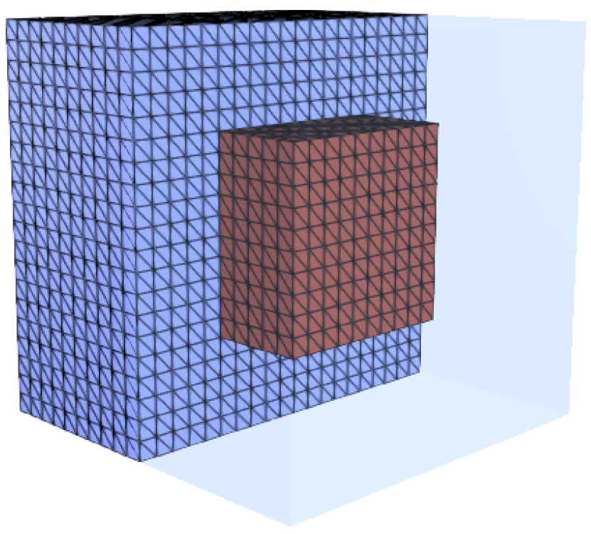
(b) 3D geometry

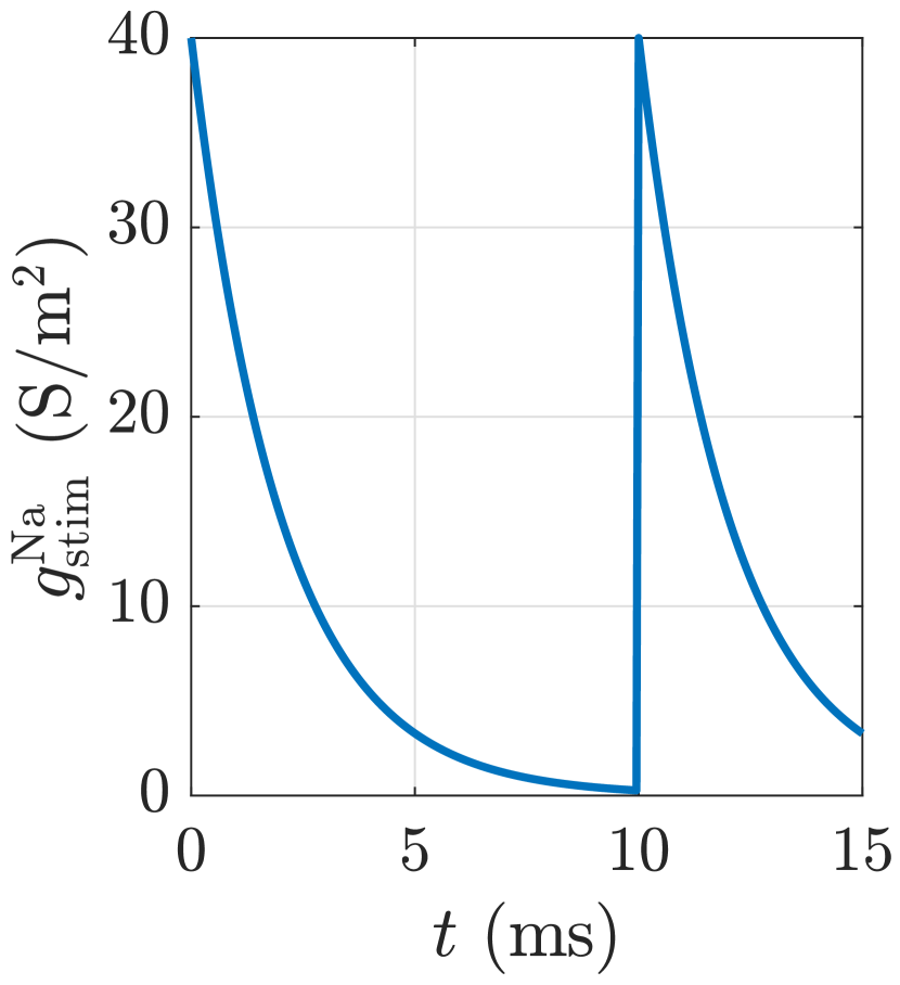
(c) Stimulus

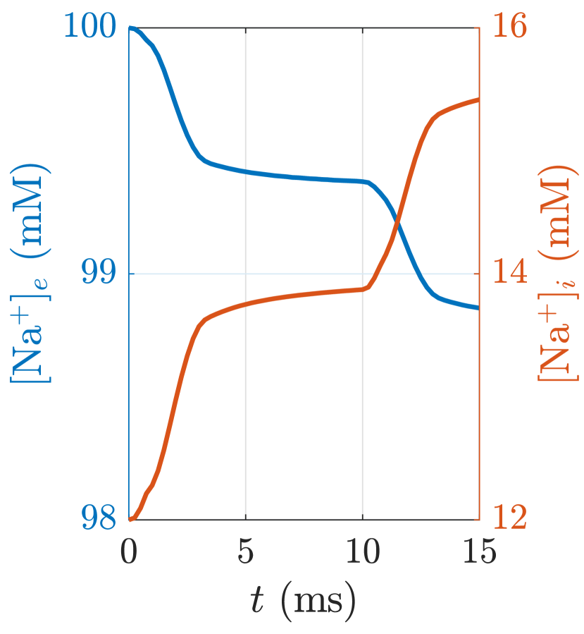
(d) Sodium

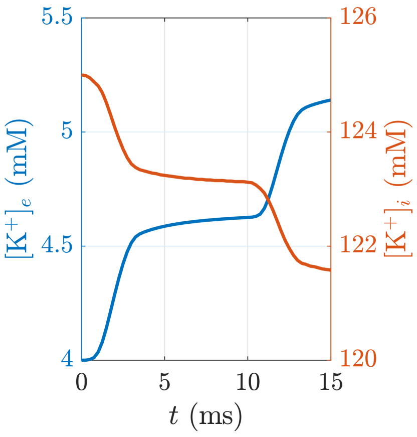
(e) Potassium

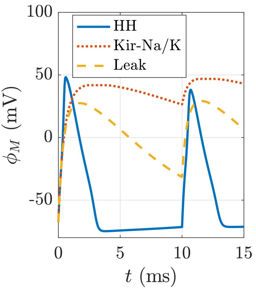
(f) Membrane potential

Figure 1: Model A. (a) Sample 2D geometry ($N_{x}=4$). (b) Sample 3D geometry ($N_{x}=20$). (c) Membrane current stimulus (acting on $\Gamma$) $g_{\rm stim}^{\rm Na}$ versus time $t$. (d) Evolution of ion concentrations over time. Extracellular and intracellular quantities are sampled respectively at $\bm{x}_{e}=(0.15,0.15)\,\mu\mathrm{m}\in\Omega_{e}$ and $\bm{x}_{i}=(0.5,0.5)\,\mu\mathrm{m}\in\Omega_{i}$. (f) Evolution of membrane potential, which is homogeneous in $\Gamma$, for different ionic models: the default Hodgkin-Huxley (HH); the Kir-Na/K model; a leak model obtained by setting $f\mathrm{{}_{Kir}}=j_{\mathrm{pump}}=0$ in the Kir-Na/K model.

5.2 Model B

We examine the electrodiffusive response of an astrocyte (a heavily branching-type of glial cell) in response to local changes in extracellular potassium and sodium concentrations resulting e.g. from surrounding neuronal activity. The intracellular astrocytic domain $\Omega_{i}$ is described by a 3D geometry obtained via Ultraliser [1, 2], with a diameter of approximately 90 $\mu$m, centered at the origin. The extracellular domain $\Omega_{e}$ is constructed as a 2 $\mu$m thick layer enclosing $\Omega_{i}$ (Figure 2(a)). The astrocytic membrane dynamics are governed by the passive Kir–Na/K membrane model (Section 2.4.2) over the entire interface $\Gamma$. As stimulus, we consider a bolus injection of potassium and removal of sodium in a section of the extracellular space over a time period of 2 ms:

$$f_{e}^{\rm Na}(\bm{x},t)=-1,\,f_{e}^{\rm K}(\bm{x},t)=1,\quad\bm{x}\in\Omega_{e}\quad\text{s.t.}\quad x<0,\quad 0<t\leq 2\,\text{ms},$$

and $f_{r}^{k}=0$ otherwise, cf. Figure 2(b). No membrane stimulus is applied ($g_{\rm stim}^{\rm Na}=0$).

The geometry is described by a tetrahedral mesh with $N_{i}=475\,206$ and $N_{e}=860\,025$ vertices, and a total problem size of $N\approx 5.3\cdot 10^{6}$ for $p=1$. Figures 2(c)–2(g) show the evolution of concentrations over time for $\Delta t=0.1$ ms and $N_{t}=2000$.

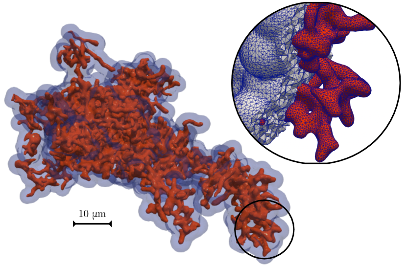
(a) Astrocyte geometry

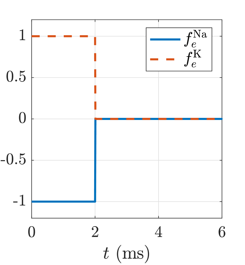
(b) Stimulus

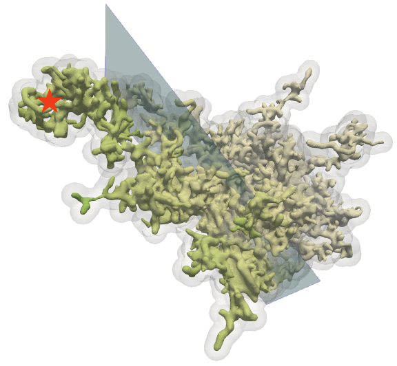
(c) [K⁺]_i at $t=30$ s and $x=0$ plane

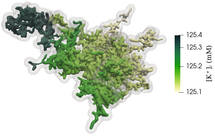
(d) [K⁺]_i at $t=200$ ms

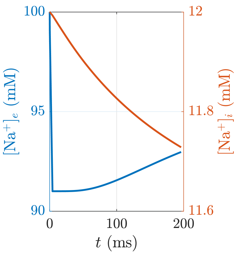
(e) Sodium

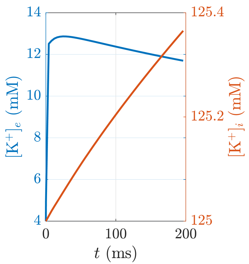
(f) Potassium

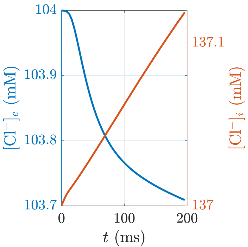
(g) Chloride

Figure 2: Model B. (a) Astrocyte geometry with corresponding tetrahedral mesh. (b) Ionic source terms over time, imposed for $x<0$. (c),(d) Intracellular potassium [K]_i (mM) at two different time steps. Potassium is injected in the extracellular space for $x<0$. At $t=2$ ms the extracellular potassium [K]_e is increased by approximately 10 mM w.r.t. the initial condition [K]${}^{0}_{e}=4$ mM. As the system evolves, potassium is electro-diffusing in both $\Omega_{i}$ and $\Omega_{e}$ through $\Gamma$. (e)–(g) Time evolution of ionic concentrations $[k]_{r}(\bm{x}_{\star},t)$ (mM) with $\bm{x}_{\star}\in\Gamma$ labeled by $\star$ in panel (c).

5.3 Model C

This model focuses on the electrodiffusive interplay between neuronal structures, the extracellular space and surrounding glial structures at the scale of dendritic spines. We consider a 3D geometry (Figure 3(a)) representing a neuronal dendrite segment with multiple dendritic spines, surrounded by extracellular space and glial cells, all immersed in a $8\times 8\times 5$ $\mu$m cuboid [33, 9]. We remark that even this highly non-trivial geometry represents a substantial simplification of the dense tissue structure, and in particular that a large number of glial structures are ignored. We apply the passive Kir–Na/K dynamics model (Section 2.4.2) at both the astrocyte–ECS and dendrite–ECS interfaces, though with $f_{\mathrm{Kir}}=j_{\mathrm{pump}}=0$ for the latter, thus in essence only considering leak channel dynamics on the dendrite–ECS interfaces. To trigger a system response, we apply sodium membrane currents at the dendritic spine heads $\Gamma_{\rm head}\subset\Gamma$ (marked in green in Figure 3(a)), mimicking synaptic signalling:

(32) $${g}^{\rm Na}_{\rm stim}(\bm{x})=\begin{cases}2\bar{g}_{\rm stim}~{}&{\text{ if }}~{}\bm{x}\in\Gamma_{\rm head},\\ 0~{}&{\text{ if }}~{}\bm{x}\notin\Gamma_{\rm head},\end{cases}$$

We consider a tetrahedral mesh with $N_{i}=193\,129$ and $N_{e}=306\,478$ vertices, and a total problem size of $N\approx 2.0\cdot 10^{6}$ for $p=1$. In Figures 3(b)–3(f), we show the resulting concentrations and potential for $N_{t}=400$ time steps and $\Delta t=0.1$ ms.

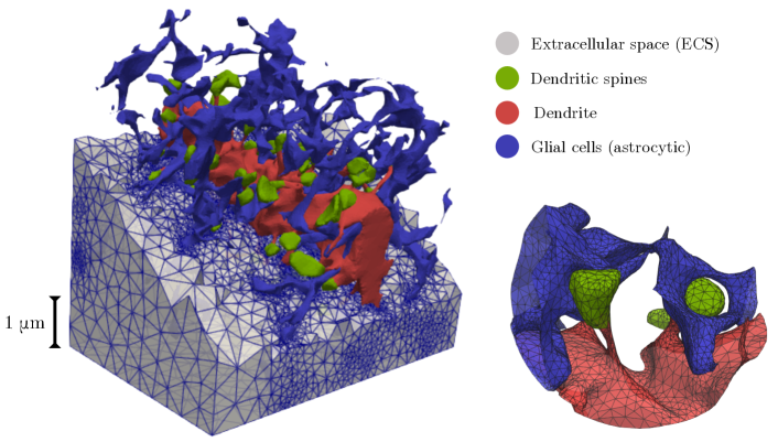
(a) Geometry

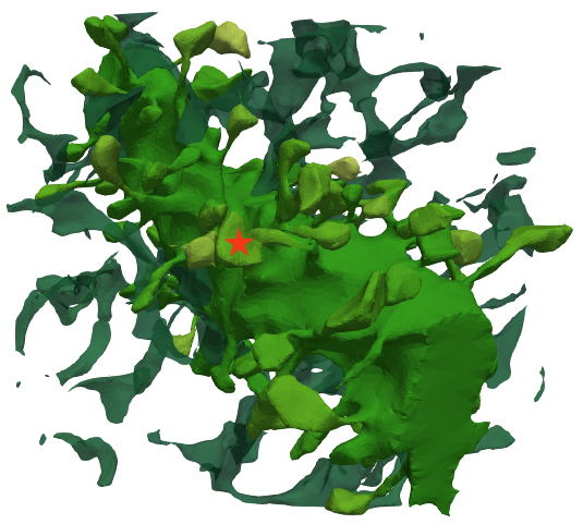
(b) [K⁺]_i in $\Gamma$ at $t=20$ ms

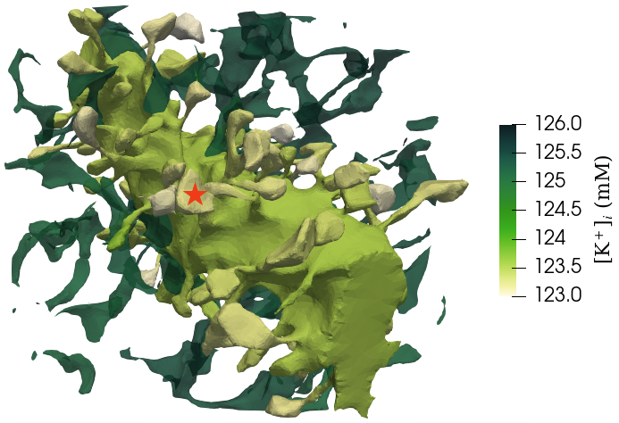
(c) [K⁺]_i in $\Gamma$ at $t=40$ ms

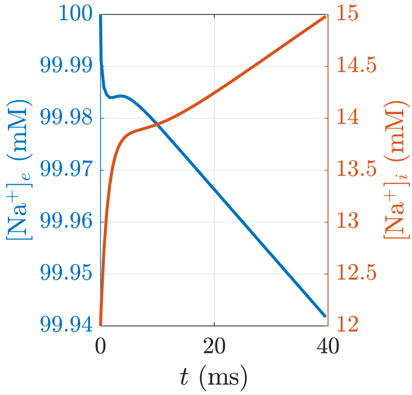
(d) Sodium

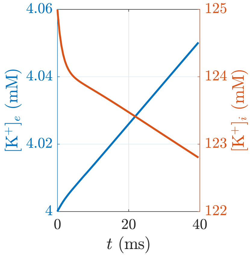
(e) Potassium

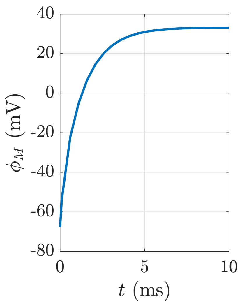
(f) Membrane potential

Figure 3: Model C. (a) Dendritic segment (red), spines heads $\Gamma_{\rm head}$ (green), and glial cells (blue). A portion of the meshed extracellular domain is shown as long as a particular of few meshed dendritic spines. (b),(c) [K]_i (mM) for two different time steps, given a membrane stimulus located in the spines heads. (d)–(f) Concentrations $[k]_{r}(\bm{x}_{\star},t)$ (mM) for $k\in\{\text{K${}^{+}$, Na${}^{+}$}\}$ and potential $\phi_{M}(\bm{x}_{\star},t)$ (mV) with $\bm{x}_{\star}\in\Gamma_{\rm head}$. The location of $\bm{x}_{\star}\in\Gamma_{\rm head}$ is labeled in panels (b) and (c) with $\star$.

5.4 Model D

We examine electrodiffusive neuronal–ECS–astrocyte interplay at a larger spatial scale. From a $100\times 100\times 80\,\mu$m portion of a rat somatosensory cortex [2, 16], we select three neurons and four astrocytes and embed these in a cuboid extracellular space (Figure 4(a)). For the neuronal membranes, we apply the active Hodgkin-Huxley model (Section 2.4.1) with a periodic, localized stimulus current

(33) $$g^{\rm Na}_{\rm stim}=10\cdot{\bar{g}}_{\rm stim}e^{-(t\,\text{mod}\,\tau)/a}\quad\text{for}\quad x<10\,\mu\text{m},$$

and ${g}^{\rm Na}_{\rm stim}=0$ otherwise. The period $\tau=10$ ms. For the astrocytic membranes, we use the passive Kir–Na/K-model as previously and ${g}^{\rm Na}_{\rm stim}=0$ (Section 2.4.2).

We consider tetrahedral meshes with up to $N_{i}=9\,390\,510$ and $N_{e}=15\,541\,672$ and problem size $N\approx 1.0\cdot 10^{8}$. The numerical solution is shown in Figures 4(b)-4(f).

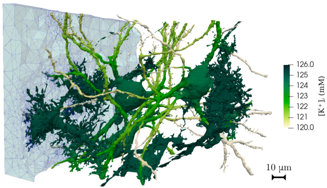
(a) Geometry and intracellular potassium in $\Gamma$ at $t=50$ ms

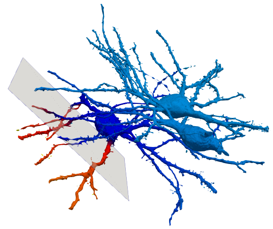
(b) Membrane potential at $t=0.5$ ms

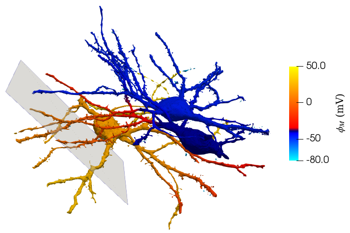
(c) Membrane potential at $t=1$ ms

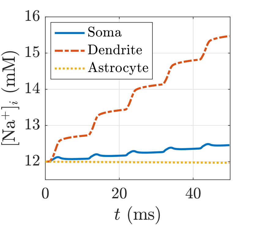
(d) Sodium

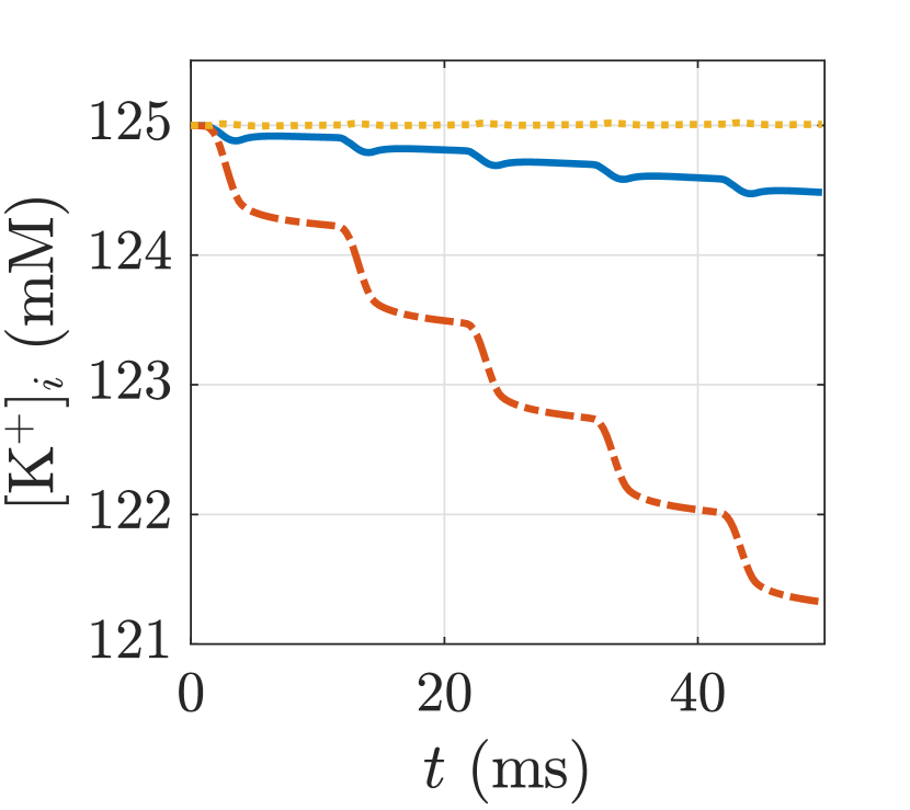
(e) Potassium

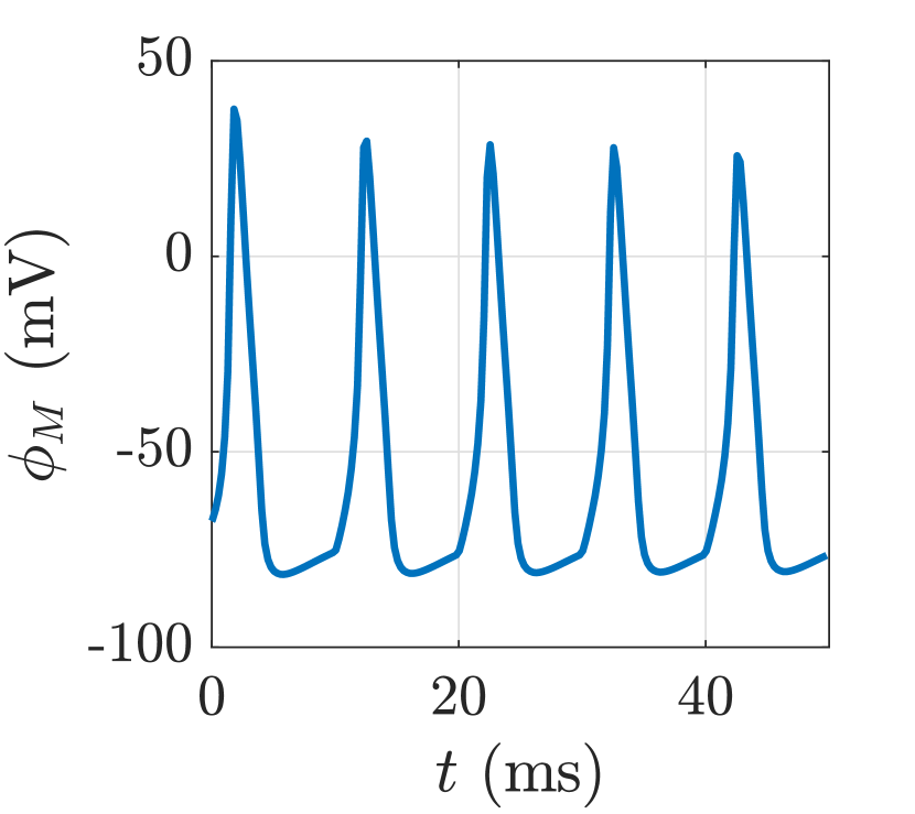
(f) Membrane potential

Figure 4: Model D. (a) Cortex geometry with neurons and astrocytes, with a portion of meshed ECS. Intracellular potassium at $t=50$ ms is shown. (b),(c) Spreading electric potential on neurons from an initial localized stimulus for two different time steps. A portion of the plane $x=10\,\mu$m is shown, as boundary of the stimulus region. A threshold potential of 40 mV is highlighted by the color scale transition. (d),(e) Intracellular concentrations for $N_{t}=1000$. The solution is sampled in the membrane of a dendrite, a soma, and an astrocyte. Legend is shared between the two images. (f) Evolution of neuronal membrane potential.

6 Numerical experiments

In this section, we examine the robustness and efficiency of the proposed monolithic numerical strategy in terms of iteration count and parallel performance when applied to Models A–C. All numerical experiments are performed on the Norwegian supercomputer Saga, using up to 256 Intel Xeon-Gold 6138/6230R 2.0-2.1 GHz CPU cores with 40 cores per node.

6.1 Implementation and numerical verification

Our KNP-EMI solver implementation [12] is based on the well-established FEniCS finite element software [5, 37], using the multiphenics library [8] to handle variational problems coupled across multiple subdomains. The linear algebra backend is PETSc [7]. The implementation is flexible in terms of ionic models of arbitrary complexity, and has been verified using the method of manufactured solutions for the same benchmark problems as introduced in [22, Section 3.1], obtaining the expected convergence rates. The image-based volumetric meshes (in Models B–D) are generated from segmented microscopy data via unions of lower-dimensional surfaces using the computational geometry library fTetWild [28].

6.2 Solver configurations

When using a GMRES method to solve the KNP-EMI system, we restart the algorithm after 30 iterations. For each time step $n$, we use the solution at $n-1$ as an initial guess, substantially reducing the number of GMRES iterations. As stopping criterion for the iterative solvers, we consider a tolerance of $10^{-6}$ for the preconditioned relative residual. To evaluate $P_{0}^{-1}$, we use a single V-cycle of hypre BoomerAMG [23]. We refer to the associated software repository [12] for the exhaustive list of AMG parameters. In terms of computational time to solve the system, the GMRES method is preferable compared to BiCGStab for all the reported experiments. For comparative tests, we also use MUMPS as a direct solver.

To solve the gating variables ODEs (cf. (17)), we use $N_{\text{ode}}=25$ intermediate time steps of the Rush-Larsen method for each time interval, set to $\Delta t=0.05$ ms (unless noted otherwise). In terms of runtime, solving the ODEs is negligible compared to the linear system solve.

6.3 Iterative solver robustness

We begin by studying the robustness of the proposed preconditioning strategy with respect to the spatial and temporal discretization. We consider a single time step for Model A, with $d=2$, as a flexible benchmark example, and vary the time step $\Delta t$, the finite element (polynomial) degree $p\in\{1,2\}$ and the mesh resolution $N_{x}\in\{16,32,64,128,256,512\}$. The resulting linear system sizes vary from $N=4.6\cdot 10^{3}$ for $(N_{x},p)=(16,1)$ to $N=4.2\cdot 10^{6}$ for $(N_{x},p)=(512,2)$. For $\Delta t\in\{1,10,100\}$ (ms), GMRES preconditioned by $P_{0}$ (LU($P_{0}$)) converges in 3 iterations for all cases. For $\Delta t\in\{0.01,0.1\}$ (ms), each case converges in 4 iterations. In contrast, the unpreconditioned GMRES method never converges in less than 1000 iterations.

Next, we investigate how to approximate $P_{0}^{-1}$ efficiently. For larger problems, it is not convenient to invert $P_{0}$ to full precision. Instead, a suitable multilevel approximation of $P_{0}^{-1}$ can reduce the time-to-solution while retaining the rapid convergence of the GMRES method. We here compare a set of such approximation strategies to black box approaches and the exact preconditioners for increasing problem sizes $N$, cf. Table 3. We immediately observe that the direct solver and ILU(0) or AMG preconditioners are not viable for larger $N$. We therefore consider two approaches where $P_{0}^{-1}$ is evaluated exactly via LU or CG (LU($P_{0}$) and CG($P_{0}$), respectively). Here, the CG solver is applied block-wise in a field-split fashion with $2(|K|+1)$ fields, and preconditioned with AMG. In both cases, the convergence behavior is dramatically improved: the number of iterations no longer increase with the problem size and remains low ($\approx 4$). However, we observe only marginal gains in terms of runtime compared to ILU(0). Finally, we consider strategies based on the multilevel approximation of $P_{0}$, obtained with a single AMG V-cycle (AMG$(P_{0})$). Besides a monolithic approach, we consider either block-wise or field-split application of AMG (AMG${}_{\text{FS}}(P_{0})$). We observe that both of these latter strategies maintain the robustness in terms of a constant and low iteration count ($\approx 4$) for all problem sizes. Moreover, we observe a significant improvement in run times for larger problem sizes. The best performance is observed for AMG applied block-wise, with a $70\%$ reduction in runtime compared to the exact preconditioner (LU($P_{0}$)).

$N$	17 412	67 588	266 244	1 056 772
($N_{x}$)	(64)	(128)	(256)	(512)
Assembly	2.5	8.2	31.3	123.3
Direct (MUMPS)	2.1	10.0	49.5	259.1
AMG	2.3 [22.5]	24.8 [61.1]	252.5 [157]	3697 [585]
ILU(0)	0.4 [15.6]	2.4 [29.5]	17.1 [63.2]	176.7 [169]
CG($P_{0}$)	3.0 [4.0]	10.5 [4.0]	39.8 [4.0]	174.4 [4.0]
LU($P_{0}$)	0.5 [4.0]	3.5 [4.0]	18.1 [4.0]	122.4 [4.0]
AMG($P_{0}$)	0.8 [4.3]	3.3 [4.1]	13.8 [4.0]	55.2 [4.0]
AMG${}_{\text{FS}}(P_{0})$	0.6 [4.0]	2.2 [4.0]	9.0 [4.0]	37.0 [4.0]

Table 3: runtimes (in serial) and when applicable, in square brackets, average number of preconditioned GMRES iterations to convergence over $n=1,\ldots,N_{t}$, for preconditioners (Model A, $p=1$, $d=2$, $N_{t}=10$ time steps). In the last two rows different inexact preconditioners are used.

We end this section by examining how the iteration counts and runtimes depend on time evolution, focusing on the two solution strategies (LU($P_{0}$) and AMG($P_{0}$)), now distributed over 32 cores (Figure 5). For both strategies, the number of iterations remains low (1–6 iterations) over the whole time span simulated. Moreover, the run time per time step (after initialization) remains bounded throughout the time course, with AMG($P_{0}$) being approximately $50\%$ faster than LU($P_{0}$) on average.

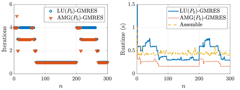
Figure 5: Number of iterations (left) and runtimes (right) over $N_{t}=300$ time steps for Model A with $d=2$ and $(N_{x},p)=(512,1)$ ($N=1\,056\,772$), using 32 MPI processes.

6.4 Parallel scalability: strong scaling

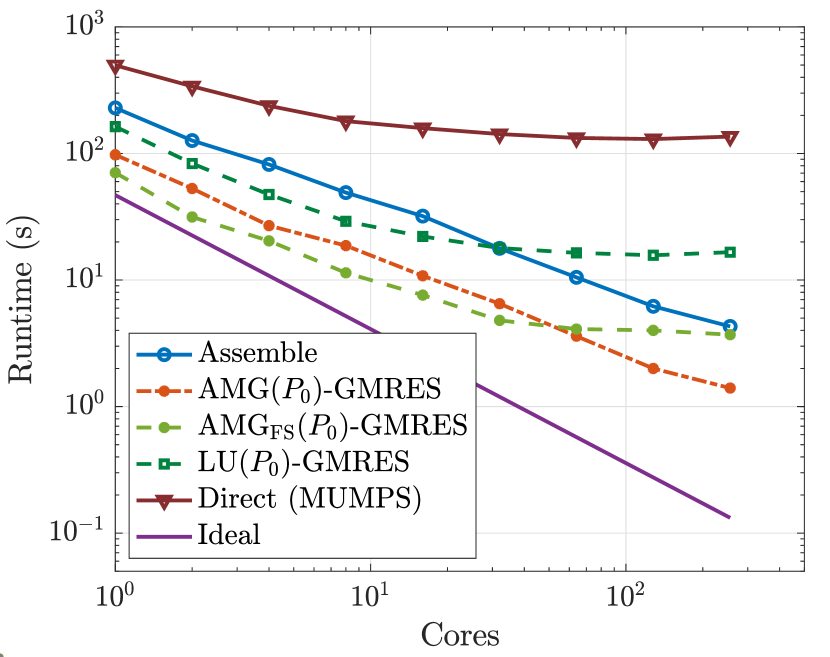
(a) Model A ($d=2$), $N=1.0\cdot 10^{6}$

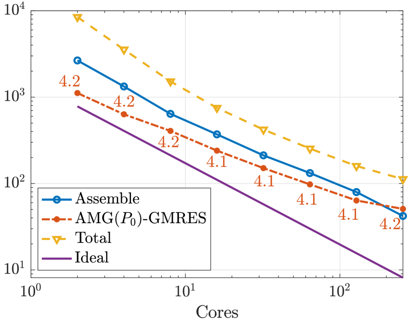
(b) Model A ($d=3$), $N=4.2\cdot 10^{6}$

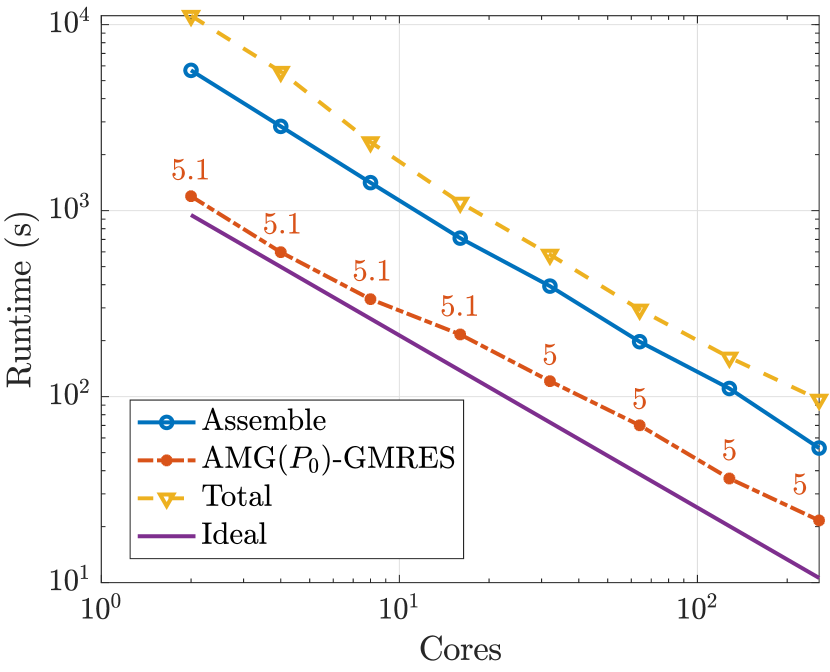
(c) Model B, $N=5.3\cdot 10^{6}$

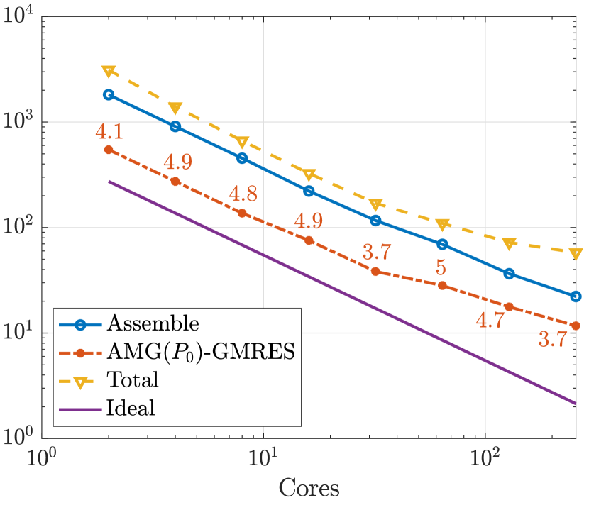
(d) Model C, $N=2.0\cdot 10^{6}$

Figure 6: Parallel performance: strong scaling for Models A, B, and C. Plots show runtimes for iterative solves, finite element assembly and total runtime versus number of MPI processes (cores). For all models, we use $p=1$ and $N_{t}=20$ time steps. Average AMG($P_{0}$)-GMRES iterations over $n=1,\ldots,N_{t}$ are indicated for each data point for Models A ($d=3$), B, and C.

We now more carefully investigate the parallel performance of the more promising preconditioned GMRES strategies (Figure 6). We first compare their strong scaling (increasing the number of cores while keeping the problem size fixed) for Models A, B, and C. For the smaller problem (Model A with $d=2$), we compare with the direct solver for reference. Throughout, we also examine the scalability of the finite element assembly. Initial tests (using Model A in 2D) indicate that all of the iterative strategies tested scale reasonably well for a few (4–8) cores (Figure 6(a)). The field-split AMG${}_{\text{FS}}(P_{0})$ is the most efficient for up to $32$ cores, but stagnates for larger core counts since each diagonal block is solved in parallel. The monolithic AMG strategy scales better and outperforms all other strategies for the Model A, $d=2$ test case for $64$ cores or more. We therefore focus our attention on the monolithic AMG in the subsequent experiments. For the larger problems (Models A with $d=3$, B and C), the scaling of AMG($P_{0}$), the assembly algorithm, and the total runtime are close to ideal for at least up to 256 cores (Figures 6(b)–6(d)). We also note that the average number of iterations remain in the same low range (4–5) varying the number of cores.

$N$	$6.7\cdot 10^{6}$	$4.5\cdot 10^{7}$	$4.5\cdot 10^{7}$	$1.0\cdot 10^{8}$
$N_{i}+N_{e}$	$1.7\cdot 10^{6}$	$1.7\cdot 10^{6}$	$1.3\cdot 10^{7}$	$2.5\cdot 10^{7}$
Finite element degree ($p$)	$1$	$2$	$1$	$1$
Initialization ($128$ cores)	20.2	60.5	335.1	991.1
Initialization ($256$ cores)	19.0	31.5	143.1	317.1
Assembly ($128$ cores)	82.5	511.5	468.4	1064.1
Assembly ($256$ cores)	44.0	278.5	263.2	547.2
AMG($P_{0}$) ($128$ cores)	20.8 [4.0]	211.6 [4.0]	132.4 [4.6]	441.8 [8.0]
AMG($P_{0}$) ($256$ cores)	12.0 [3.9]	111.5 [3.9]	64.9 [3.9]	242.9 [7.8]

Table 4: Scalability and performance for Model D. Computational runtimes and, in square brackets, average number of iterations to convergence over $n=1,\ldots,N_{t}=10$ time steps. Total number of degrees of freedom $N$, intracellular and extracellular degrees of freedom $N_{i}+N_{e}$, finite element (polynomial) degree $p$, with rows corresponding to 128 and 256 MPI processes as labeled. The initialization time corresponds to the finite element discretization setup in the first time step, thus becoming negligible for large $N_{t}$. The columns give (from left to right) the results corresponding to Model D with: (i) $p=1$, (ii) $p=2$, (iii) after uniform mesh refinement, and (iv) after uniform and then interface-based mesh refinement.

We also conduct a focused larger-scale experiment using Model D with up to $10^{8}$ degrees of freedom to study the effect of bulk- versus interface-dominated mesh refinement on algorithmic and parallel performance (Table 4). As a baseline, we consider Model D with the default configuration (Table 4, first column), as described in Section 5, for 128 and 256 cores. For the case $p=2$ (Table 4, second column) with a $6.8\times$ increase in the number of degrees of freedom and reduced sparsity, assembly time increases by a factor of $6.3\times$, while the linear solver time increases by a factor of $9.3\times$. On the other hand, after uniform mesh refinement (third column), which yields the same increase in $N$ and same sparsity pattern, the assembly time increases by a factor of $5.7\times$ (128 cores) and $6.0\times$ (256 cores), while the GMRES runtime increases by $6.3\times$ and $5.4\times$, demonstrating near-optimal or super-optimal scalability with respect to $N$. For both cases, we again observe that the average number of GMRES iterations stays near constant, remaining at 4–5.

Finally, we study the effect of refining the mesh near the interface $\Gamma$ only. This scenario challenges the spectral analysis [10] in which the robustness of the preconditioning strategy eliminating membrane blocks is established under the assumption of uniform refinement. Indeed, the average number of iterations now increases, from 4–5 to 8, with a corresponding increase in computational cost (comparing the third and fourth columns of Table 4). For all four columns, both the finite element assembly and the AMG($P_{0}$)-GMRES solver scale near-optimally when increasing from 128 to 256 cores, with an average parallel efficiency of $93\%$ and $94\%$ respectively.

6.5 Parallel scalability: weak scaling

Finally, we investigate the weak scaling (increasing the number of cores and the problem size simultaneously) of the various solution strategies, returning again to Model A (Figure 7). For small-sized problems (Figure 7, left), the field-split AMG${}_{\text{FS}}(P_{0})$-GMRES is the fastest in serial, but, again, the monolithic AMG($P_{0}$) outperforms all the other approaches in terms of scaling. For the moderate-sized problems (Figure 7(b), right), near optimal scalability is observed for the assembly, with essentially a flat curve from 64 to 256 cores. As expected, the number of AMG($P_{0}$)-GMRES iterations stays near constant ($\approx 4$), while its runtime increases by an average factor of $1.2\times$ as the number of cores and degrees of freedom doubles. The increase in runtime is connected to communication overhead in matrix-vector products and AMG setup. We refer to [18] for examples of fine tuning AMG parameters to further improve its weak scalability.

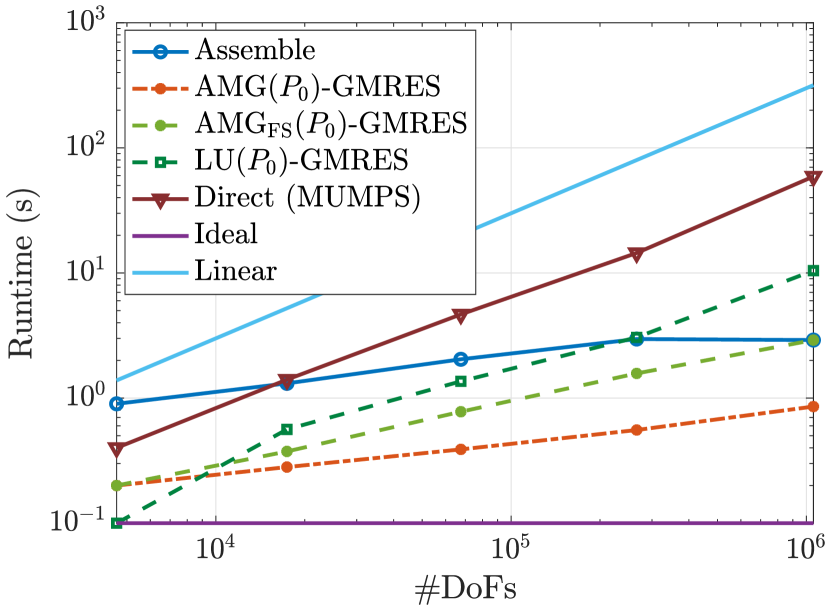
(a) Model A ($d=2$)

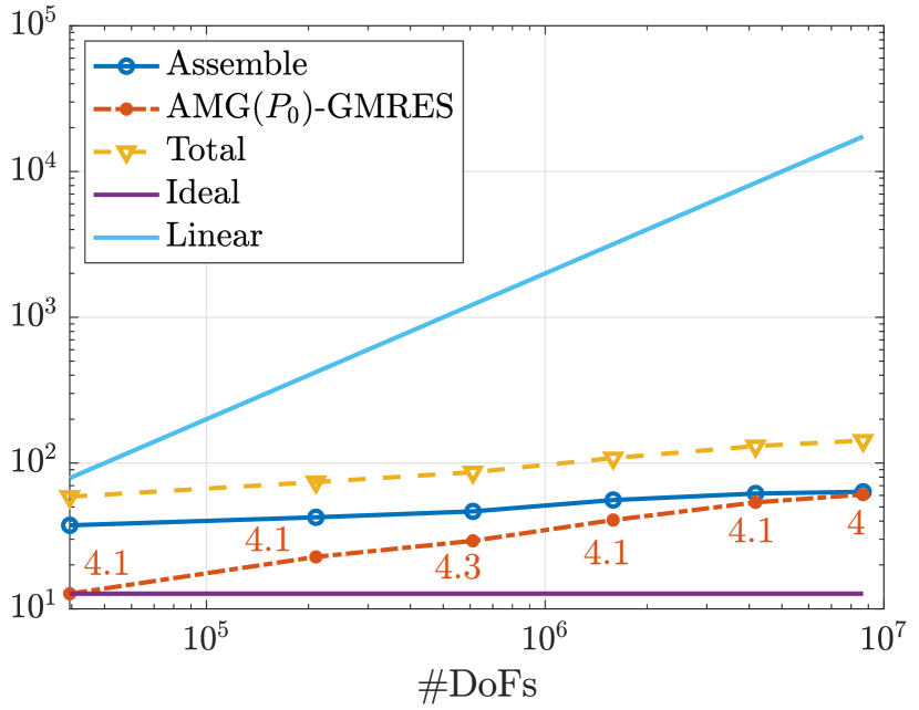
(b) Model A ($d=3$)

Figure 7: Parallel performance: weak scaling for Model A ($p=1$) with (a) $d=2$, $N_{t}=10$, $4.5\cdot 10^{3}$ degrees of freedom per core and (b) $d=3$ and $N_{t}=20$, and $4.0\cdot 10^{4}$ degrees of freedom per core. Average AMG($P_{0}$)-GMRES iterations over $n=1,\ldots,N_{t}$ are displayed as well as the total runtime.

7 Discussion, conclusions and outlook

The availability of dense brain tissue reconstructions at an extreme level of detail poses a unique challenge for mathematical and computational modelling. Here, we presented a scalable finite element discretization and solution algorithm to solve the KNP-EMI equations, describing electrodiffusion, at the level of complexity required for physiologically relevant simulations. In particular, we employ a continuous finite elements discretization of arbitrary order, with possible discontinuities across interfaces, where the KNP-EMI equations are coupled with one or more ODEs, modeling complex membrane dynamics. We describe the algebraic structure of the arising monolithic linear system and present a tailored multilevel solution strategy, since black-box approaches are unfeasible for large problems.

We show robustness of the our proposed solution strategy with respect to discretization parameters, given a near uniform spatial refinement. Strong and weak scalability of the algorithm are near-optimal, as demonstrated here when running simulations using from 1 to 256 MPI processes for problem sizes ranging from $4.6\cdot 10^{3}$ to $10^{8}$. Our motivation for considering this range of parallelism is four-fold: (i) these problem sizes represent the first relevant stage for resolving the brain tissue geometry at the tens of micrometers scale; (ii) any viable solution strategy must successfully address this range; (iii) this is a range of computing resources readily available, in particular 256 represents the default core limit for the Saga computing system; and (iv) above these problem sizes, other aspects of the simulation pipeline such as e.g., mesh generation, labeling, and refinement appear as non-negligible potential bottlenecks. However, our numerical results indicate that the solution algorithm can continue to scale for larger problem sizes and a larger core count. We also remark that while we have presented physiologically relevant scenarios, more complexity could, and should, be considered. For instance, more attention to the connectedness or non-connectedness of the extracellular space and intracellular compartments could yield even higher fidelity representations. Similarly, while we here consider different non-trivial membrane mechanisms for the different cellular types, a higher degree of specificity would be more biologically meaningful, in particular for the neuronal compartments (axons, soma, dendrites). Our simulation code is openly available [12], and importantly, we envision that the model scenarios presented can be used as stepping stones for future benchmarks and research in this emerging field.

Data availability

This manuscript is accompanied by open software and data sets available at https://doi.org/10.5281/zenodo.10728462 [12].

Conflict of interest

The authors declare that they have no conflict of interest.

References

- [1] M. Abdellah, J. J. G. Cantero, N. R. Guerrero, A. Foni, J. S. Coggan, C. Calì, M. Agus, E. Zisis, D. Keller, M. Hadwiger, et al., Ultraliser: a framework for creating multiscale, high-fidelity and geometrically realistic 3D models for in silico neuroscience, Briefings in Bioinformatics, 24 (2023), p. bbac491.
- [2] M. Abdellah, J. J. G. Cantero, N. R. Guerrero, A. Foni, J. S. Coggan, C. Calì, M. Agus, E. Zisis, D. Keller, M. Hadwiger, P. J. Magistretti, H. Markram, and F. Schürmann, Ultraliser: a framework for creating multiscale, high-fidelity and geometrically realistic 3D models for in silico neuroscience, Sept. 2022, https://doi.org/10.5281/zenodo.7105941, https://doi.org/10.5281/zenodo.7105941.
- [3] A. Agudelo-Toro and A. Neef, Computationally efficient simulation of electrical activity at cell membranes interacting with self-generated and externally imposed electric fields, Journal of neural engineering, 10 (2013), p. 026019.
- [4] P. Aitken and G. Somjen, The sources of extracellular potassium accumulation in the CA1 region of hippocampal slices, Brain research, 369 (1986), pp. 163–167.
- [5] M. Alnæs, J. Blechta, J. Hake, A. Johansson, B. Kehlet, A. Logg, C. Richardson, J. Ring, M. E. Rognes, and G. N. Wells, The FEniCS project version 1.5, Archive of Numerical Software, 3 (2015).
- [6] M. Armbruster, S. Naskar, J. P. Garcia, M. Sommer, E. Kim, Y. Adam, P. G. Haydon, E. S. Boyden, A. E. Cohen, and C. G. Dulla, Neuronal activity drives pathway-specific depolarization of peripheral astrocyte processes, Nature neuroscience, 25 (2022), pp. 607–616.
- [7] S. Balay, S. Abhyankar, M. F. Adams, S. Benson, J. Brown, P. Brune, K. Buschelman, E. M. Constantinescu, L. Dalcin, A. Dener, V. Eijkhout, J. Faibussowitsch, W. D. Gropp, V. Hapla, T. Isaac, P. Jolivet, D. Karpeev, D. Kaushik, M. G. Knepley, F. Kong, S. Kruger, D. A. May, L. C. McInnes, R. T. Mills, L. Mitchell, T. Munson, J. E. Roman, K. Rupp, P. Sanan, J. Sarich, B. F. Smith, S. Zampini, H. Zhang, H. Zhang, and J. Zhang, PETSc Web page. https://petsc.org/, 2023, https://petsc.org/.
- [8] F. Ballarin, multiphenics, 2024, https://multiphenics.github.io/.
- [9] T. M. Bartol, D. X. Keller, J. P. Kinney, C. L. Bajaj, K. M. Harris, T. J. Sejnowski, and M. B. Kennedy, Computational reconstitution of spine calcium transients from individual proteins, Frontiers in synaptic neuroscience, 7 (2015), p. 17.
- [10] P. Benedusi, P. Ferrari, C. Garoni, R. Krause, and S. Serra-Capizzano, Fast parallel solver for the space-time IgA-DG discretization of the diffusion equation, Journal of Scientific Computing, 89 (2021), p. 20.
- [11] P. Benedusi, P. Ferrari, M. Rognes, and S. Serra-Capizzano, Modeling excitable cells with the EMI equations: spectral analysis and iterative solution strategy, Journal of Scientific Computing, 98 (2024), p. 58.
- [12] P. Benedusi and M. E. Rognes, Scalable approximation and solvers for ionic electrodiffusion in cellular geometries, 2024, https://doi.org/https://doi.org/10.5281/zenodo.10728462.
- [13] N. Berre, M. E. Rognes, and A. Massing, Cut finite element discretizations of cell-by-cell EMI electrophysiology models, arXiv preprint arXiv:2306.03001, (2023).
- [14] W. F. Boron and E. L. Boulpaep, Medical physiology, Elsevier Health Sciences, 2016.
- [15] A. P. Buccino, M. Kuchta, J. Schreiner, and K.-A. Mardal, Improving neural simulations with the EMI model, in Modeling Excitable Tissue, Springer, 2021, pp. 87–98.
- [16] C. Calì, M. Agus, K. Kare, D. J. Boges, H. Lehväslaiho, M. Hadwiger, and P. J. Magistretti, 3D cellular reconstruction of cortical glia and parenchymal morphometric analysis from serial block-face electron microscopy of juvenile rat, Progress in neurobiology, 183 (2019), p. 101696.
- [17] M. Consortium, J. A. Bae, M. Baptiste, C. A. Bishop, A. L. Bodor, D. Brittain, J. Buchanan, D. J. Bumbarger, M. A. Castro, B. Celii, et al., Functional connectomics spanning multiple areas of mouse visual cortex, BioRxiv, (2021), pp. 2021–07.
- [18] P. D’Ambra, F. Durastante, and S. Filippone, AMG preconditioners for linear solvers towards extreme scale, SIAM Journal on Scientific Computing, 43 (2021), pp. S679–S703.
- [19] E. J. Dickinson, J. G. Limon-Petersen, and R. G. Compton, The electroneutrality approximation in electrochemistry, Journal of Solid State Electrochemistry, 15 (2011), pp. 1335–1345.
- [20] A. G. Dietz, P. Weikop, N. Hauglund, M. Andersen, N. C. Petersen, L. Rose, H. Hirase, and M. Nedergaard, Local extracellular K+ in cortex regulates norepinephrine levels, network state, and behavioral output, Proceedings of the National Academy of Sciences, 120 (2023), p. e2305071120.
- [21] A. J. Ellingsrud, N. Boullé, P. E. Farrell, and M. E. Rognes, Accurate numerical simulation of electrodiffusion and water movement in brain tissue, Mathematical Medicine and Biology: A Journal of the IMA, 38 (2021), pp. 516–551.
- [22] A. J. Ellingsrud, A. Solbrå, G. T. Einevoll, G. Halnes, and M. E. Rognes, Finite element simulation of ionic electrodiffusion in cellular geometries, Frontiers in Neuroinformatics, 14 (2020), p. 11.
- [23] R. D. Falgout and U. M. Yang, hypre: A library of high performance preconditioners, in Computational Science—ICCS 2002: International Conference Amsterdam, The Netherlands, April 21–24, 2002 Proceedings, Part III, Springer, 2002, pp. 632–641.
- [24] S. Farina, S. Claus, J. S. Hale, A. Skupin, and S. P. Bordas, A cut finite element method for spatially resolved energy metabolism models in complex neuro-cell morphologies with minimal remeshing, Advanced Modeling and Simulation in Engineering Sciences, 8 (2021), pp. 1–32.
- [25] G. Halnes, I. Østby, K. H. Pettersen, S. W. Omholt, and G. T. Einevoll, Electrodiffusive model for astrocytic and neuronal ion concentration dynamics, PLoS computational biology, 9 (2013), p. e1003386.
- [26] B. Hille et al., Ion channels of excitable membranes, vol. 507, Sinauer Sunderland, MA, 2001.
- [27] A. L. Hodgkin and A. F. Huxley, A quantitative description of membrane current and its application to conduction and excitation in nerve, The Journal of physiology, 117 (1952), p. 500.
- [28] Y. Hu, T. Schneider, B. Wang, D. Zorin, and D. Panozzo, Fast tetrahedral meshing in the wild, ACM Trans. Graph., 39 (2020), https://doi.org/10.1145/3386569.3392385, https://doi.org/10.1145/3386569.3392385.
- [29] N. M. M. Huynh, F. Chegini, L. F. Pavarino, M. Weiser, and S. Scacchi, Convergence analysis of BDDC preconditioners for composite dg discretizations of the cardiac cell-by-cell model, SIAM Journal on Scientific Computing, 45 (2023), pp. A2836–A2857.
- [30] K. H. Jæger, A. G. Edwards, W. R. Giles, and A. Tveito, Arrhythmogenic influence of mutations in a myocyte-based computational model of the pulmonary vein sleeve, Scientific Reports, 12 (2022), p. 7040.
- [31] K. H. Jæger, K. G. Hustad, X. Cai, and A. Tveito, Efficient numerical solution of the EMI model representing the extracellular space (e), cell membrane (m) and intracellular space (i) of a collection of cardiac cells, Frontiers in Physics, 8 (2021), p. 579461.
- [32] M. Kespe, S. Cernak, M. Gleiß, S. Hammerich, and H. Nirschl, Three-dimensional simulation of transport processes within blended electrodes on the particle scale, International Journal of Energy Research, 43 (2019), pp. 6762–6778.
- [33] J. P. Kinney, J. Spacek, T. M. Bartol, C. L. Bajaj, K. M. Harris, and T. J. Sejnowski, Extracellular sheets and tunnels modulate glutamate diffusion in hippocampal neuropil, Journal of Comparative Neurology, 521 (2013), pp. 448–464.
- [34] M. Kuchta, K.-A. Mardal, and M. E. Rognes, Solving the emi equations using finite element methods, Modeling Excitable Tissue: The EMI Framework, (2021), pp. 56–69.
- [35] T. Lagache, K. Jayant, and R. Yuste, Electrodiffusion models of synaptic potentials in dendritic spines, Journal of computational neuroscience, 47 (2019), pp. 77–89.
- [36] C. T. Lee, J. G. Laughlin, N. Angliviel de La Beaumelle, R. E. Amaro, J. A. McCammon, R. Ramamoorthi, M. Holst, and P. Rangamani, 3D mesh processing using GAMer 2 to enable reaction-diffusion simulations in realistic cellular geometries, PLoS computational biology, 16 (2020), p. e1007756.
- [37] A. Logg, K.-A. Mardal, and G. Wells, Automated solution of differential equations by the finite element method: The FEniCS book, vol. 84, Springer Science & Business Media, 2012.
- [38] Y. Mori, A multidomain model for ionic electrodiffusion and osmosis with an application to cortical spreading depression, Physica D: Nonlinear Phenomena, 308 (2015), pp. 94–108.
- [39] Y. Mori and C. Peskin, A numerical method for cellular electrophysiology based on the electrodiffusion equations with internal boundary conditions at membranes, Communications in Applied Mathematics and Computational Science, 4 (2009), pp. 85–134, http://dx.doi.org/10.2140/camcos.2009.4.85.
- [40] A. Motta, M. Berning, K. M. Boergens, B. Staffler, M. Beining, S. Loomba, P. Hennig, H. Wissler, and M. Helmstaedter, Dense connectomic reconstruction in layer 4 of the somatosensory cortex, Science, 366 (2019).
- [41] C. Nicholson, G. Ten Bruggencate, H. Stockle, and R. Steinberg, Calcium and potassium changes in extracellular microenvironment of cat cerebellar cortex, Journal of neurophysiology, 41 (1978), pp. 1026–1039.
- [42] S. Niederer, Regulation of ion gradients across myocardial ischemic border zones: a biophysical modelling analysis, PloS one, 8 (2013), p. e60323.
- [43] M. S. Nordentoft, A. Papoutsi, N. Takahashi, M. S. Heltberg, M. H. Jensen, and R. N. Rasmussen, Local changes in potassium ions modulate dendritic integration, bioRxiv, (2023), pp. 2023–05.
- [44] J. Pods, J. Schönke, and P. Bastian, Electrodiffusion models of neurons and extracellular space using the Poisson-Nernst-Planck equations—numerical simulation of the intra-and extracellular potential for an axon model, Biophysical journal, 105 (2013), pp. 242–254.
- [45] R. Rasmussen, J. O’Donnell, F. Ding, and M. Nedergaard, Interstitial ions: A key regulator of state-dependent neural activity?, Progress in Neurobiology, (2020), p. 101802.
- [46] G. Rosilho de Souza, R. Krause, S. Pezzuto, et al., Boundary integral formulation of the cell-by-cell model of cardiac electrophysiology, Engineering Analysis with Boundary Elements, 158 (2024), pp. 239–251.
- [47] T. Roy, J. Andrej, and V. A. Beck, A scalable DG solver for the electroneutral Nernst-Planck equations, Journal of Computational Physics, 475 (2023), p. 111859.
- [48] M. J. Sætra, G. T. Einevoll, and G. Halnes, An electrodiffusive neuron-extracellular-glia model for exploring the genesis of slow potentials in the brain, PLoS Computational Biology, 17 (2021), p. e1008143.
- [49] M. J. Sætra, A. J. Ellingsrud, and M. E. Rognes, Neural activity induces strongly coupled electro-chemo-mechanical interactions and fluid flow in astrocyte networks and extracellular space–a computational study, PLOS Computational Biology, (2023), https://doi.org/10.1371/journal.pcbi.1010996.
- [50] S. Shirinpour, N. Hananeia, J. Rosado, H. Tran, C. Galanis, A. Vlachos, P. Jedlicka, G. Queisser, and A. Opitz, Multi-scale modeling toolbox for single neuron and subcellular activity under transcranial magnetic stimulation, Brain stimulation, 14 (2021), pp. 1470–1482.
- [51] A. Solbrå, A. W. Bergersen, J. van den Brink, A. Malthe-Sørenssen, G. T. Einevoll, and G. Halnes, A Kirchhoff-Nernst-Planck framework for modeling large scale extracellular electrodiffusion surrounding morphologically detailed neurons, PLoS computational biology, 14 (2018), p. e1006510.
- [52] D. Sterratt, B. Graham, A. Gillies, G. Einevoll, and D. Willshaw, Principles of computational modelling in neuroscience, Cambridge University Press, 2023, https://doi.org/10.1017/CBO9780511975899.
- [53] J. Sundnes, B. F. Nielsen, K. A. Mardal, X. Cai, G. T. Lines, and A. Tveito, On the computational complexity of the bidomain and the monodomain models of electrophysiology, Annals of biomedical engineering, 34 (2006), pp. 1088–1097.
- [54] A. Tveito, K. H. Jæger, M. Kuchta, K.-A. Mardal, and M. E. Rognes, A cell-based framework for numerical modeling of electrical conduction in cardiac tissue, Frontiers in Physics, 5 (2017), p. 48.
- [55] A. Tveito, K.-A. Mardal, and M. E. Rognes, Modeling excitable tissue: the EMI framework, Springer, 2021.
- [56] V. Untiet, F. R. Beinlich, P. Kusk, N. Kang, A. Ladrón-de Guevara, W. Song, C. Kjaerby, M. Andersen, N. Hauglund, Z. Bojarowska, et al., Astrocytic chloride is brain state dependent and modulates inhibitory neurotransmission in mice, Nature Communications, 14 (2023), p. 1871.
- [57] C. Voßen, J. P. Eberhard, and G. Wittum, Modeling and simulation for three-dimensional signal propagation in passive dendrites, Computing and Visualization in Science, 10 (2007), pp. 107–121.
- [58] K. Xylouris, G. Queisser, and G. Wittum, A three-dimensional mathematical model of active signal processing in axons, Computing and visualization in science, 13 (2010), pp. 409–418.
- [59] K. Xylouris and G. Wittum, A three-dimensional mathematical model for the signal propagation on a neuron’s membrane, Frontiers in computational neuroscience, 9 (2015), p. 94.
- [60] H. Yang, Z. Qian, J. Wang, J. Feng, C. Tang, L. Wang, Y. Guo, Z. Liu, Y. Yang, K. Zhang, et al., Carbon nanotube array-based flexible multifunctional electrodes to record electrophysiology and ions on the cerebral cortex in real time, Advanced Functional Materials, 32 (2022), p. 2204794.
- [61] L. Yao and Y. Mori, A numerical method for osmotic water flow and solute diffusion with deformable membrane boundaries in two spatial dimension, Journal of Computational Physics, 350 (2017), pp. 728–746.
- [62] E. Zisis, D. Keller, L. Kanari, A. Arnaudon, M. Gevaert, T. Delemontex, B. Coste, A. Foni, A. Marwan, C. Calì, et al., Architecture of the neuro-glia-vascular system, bioRxiv 2021.01.19.427241, (2021).