Disentangled Diffusion-Based 3D Human Pose Estimation with
Hierarchical Spatial and Temporal Denoiser

Abstract

Recently, diffusion-based methods for monocular 3D human pose estimation have achieved state-of-the-art (SOTA) performance by directly regressing the 3D joint coordinates from the 2D pose sequence. Although some methods decompose the task into bone length and bone direction prediction based on the human anatomical skeleton to explicitly incorporate more human body prior constraints, the performance of these methods is significantly lower than that of the SOTA diffusion-based methods. This can be attributed to the tree structure of the human skeleton. Direct application of the disentangled method could amplify the accumulation of hierarchical errors, propagating through each hierarchy. Meanwhile, the hierarchical information has not been fully explored by the previous methods. To address these problems, a Disentangled Diffusion-based 3D Human Pose Estimation method with Hierarchical Spatial and Temporal Denoiser is proposed, termed DDHPose. In our approach: (1) We disentangle the 3D pose and diffuse the bone length and bone direction during the forward process of the diffusion model to effectively model the human pose prior. A disentanglement loss is proposed to supervise diffusion model learning. (2) For the reverse process, we propose Hierarchical Spatial and Temporal Denoiser (HSTDenoiser) to improve the hierarchical modeling of each joint. Our HSTDenoiser comprises two components: the Hierarchical-Related Spatial Transformer (HRST) and the Hierarchical-Related Temporal Transformer (HRTT). HRST exploits joint spatial information and the influence of the parent joint on each joint for spatial modeling, while HRTT utilizes information from both the joint and its hierarchical adjacent joints to explore the hierarchical temporal correlations among joints. Extensive experiments on the Human3.6M and MPI-INF-3DHP datasets show that our method outperforms the SOTA disentangled-based, non-disentangled based, and probabilistic approaches by 10.0%, 2.0%, and 1.3%, respectively.

Introduction

3D Human Pose Estimation (HPE) has crucial applications in virtual reality  (Hagbi et al. 2010), human motion recognition  (Zhang et al. 2022b), and human-computer interaction  (Kisacanin, Pavlovic, and Huang 2005). The goal is to regress the 3D joints locations of a human in the 3D space using the input of 2D pose sequence. Most of the methods first derive predictions of 2D joints using estimators such as HRNet (Wang et al. 2020), CPN (Chen et al. 2018), OpenPose (Cao et al. 2017) and AlphaPose (Fang et al. 2017), and then perform 2D-to-3D lifting to obtain the final estimation results.

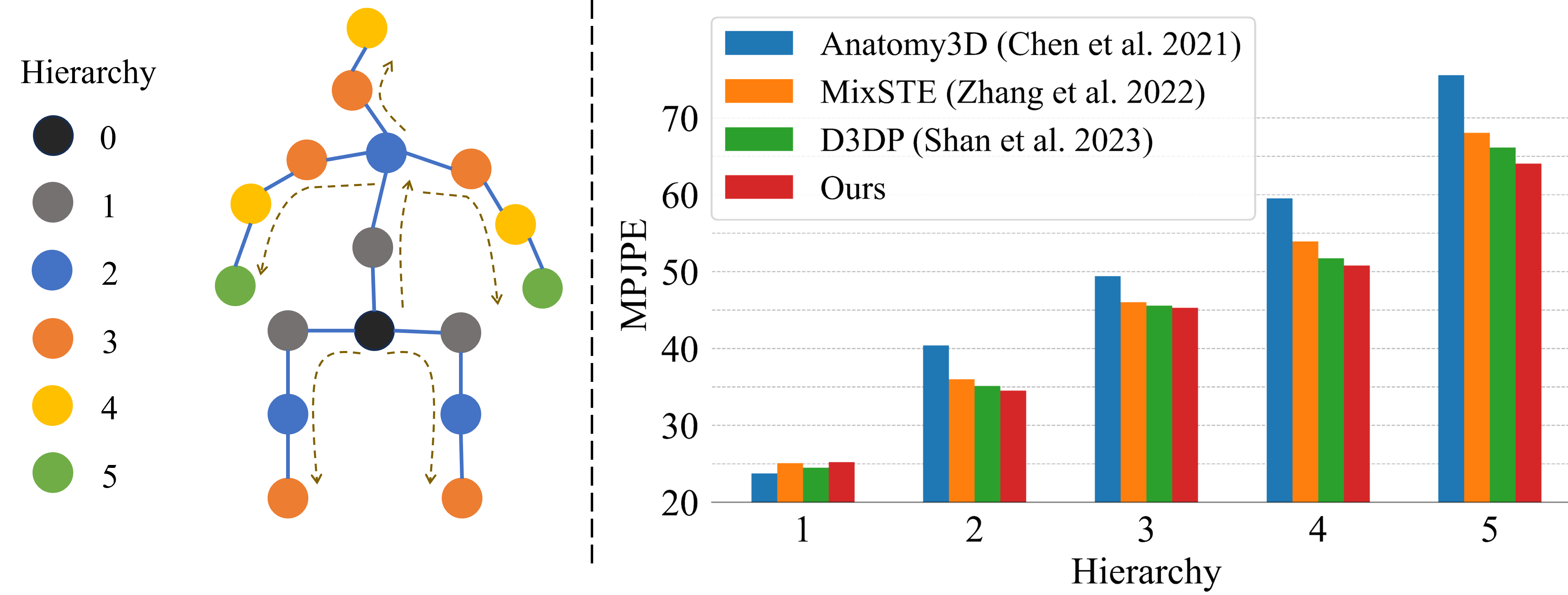
Figure 1: Left: The hierarchy defined in our method and the forward kinematic structure (drawn with brown dashed lines) based on the Human3.6M dataset. Right: The MPJPE of the hierarchy 1-5 joints comparison among Anatomy3D  (Chen et al. 2021), MixSTE  (Zhang et al. 2022a), D3DP  (Shan et al. 2023) and our method.

Recently, monocular 3D human pose estimation has experienced significant advancements. Many methods have been proposed to alleviate the depth ambiguity.  (Pavllo et al. 2019) considers this issue by exploring temporal information with the convolutional network while the transformer-based methods  (Zheng et al. 2021; Zhang et al. 2022a) make use of spatial-temporal information to compensate for the information loss in the 2D to 3D mapping process. Learning or introducing human pose prior is another method to mitigate the depth ambiguity.  (Shan et al. 2023; Ci et al. 2023; Gong et al. 2023) introduce the original pose distribution prior in the training phase, and model 2D-to-3D lifting as a process to denoise from the pose distribution with uncertain noise. Moreover, some disentangle-based methods like  (Xu et al. 2020; Chen et al. 2021; Wang et al. 2022) explicitly predict the bone length and bone direction, subsequently composing 3D joints locations based on the forward kinematics of the human skeleton. Such methods employ explicit pose constraints, integrating symmetry loss, joint angle limits  (Xu et al. 2020), and the consistent bone length in the videos  (Chen et al. 2021).

However, there are two problems existing in these methods: (1) Despite the advantages of disentangle-based techniques in incorporating human pose priors, they come with the drawback of amplified error accumulation, resulting in decreased performance. Meanwhile, diffusion-based 3D HPE methods  (Shan et al. 2023; Ci et al. 2023; Gong et al. 2023) directly add noise to the original 3D pose which is not conducive to learn the explicit human pose prior. What if we disentangle the diffusion model by adding noise to bone length and direction separately? This disentangle-based model can separately focus on the temporal consistency of bone length and joint angle variations, better enabling the diffusion model to learn human pose prior. (2) Although the transformer-based methods have the ability to explore the spatial-temporal context information, these models generally lack attention to the fine-grained hierarchical information among joints. As shown in the left side of Figure 1, we group joints into six hierarchies based on the kinematic tree depth of the human body. The experiment results in the right side of Figure 1 show a rising hierarchical accumulation error when the hierarchy increases from 1 to 5.

To solve the problems mentioned above, (1) we introduce the disentangled method in the forward process of diffusion model instead of decomposing the 3D HPE task into bone length and bone direction prediction task, which simplifies learning the human pose prior. (2) For better modeling the hierarchical relation among joints, we propose HSTDenoiser, which contains two modules: the Hierarchical-Related Spatial Transformer (HRST) and the Hierarchical-Related Temporal Transformer (HRTT). In HRST, due to the spatial information of a joint is influenced by its parent joint, we supply the joint’s attention with information from its parent joint. Besides, in HRTT, we try to make cross-attention of the joint and the adjacent joints to learn the temporal interrelationships. HRST and HRTT make the joints pay more attention to their hierarchical-related joints, which consequently improves performance on higher-hierarchy joints and contributes to overall better performance.

In conclusion, our contributions can be summarized as follows:

• We propose the first Disentangled Diffusion-based 3D human Pose Estimation method with Hierarchical Spatial and Temporal Denoiser (DDHPose), which introduces Hierarchical Information in two ways.

• We present the Disentangle Strategy for the forward diffusion process based on hierarchical information to better model explicit pose prior. Additionally, we incorporate a disentanglement loss to guide the model’s training.

• The HSTDenoiser is introduced, comprising the Hierarchical-Related Spatial Transformer (HRST) and the Hierarchical-Related Temporal Transformer (HRTT). This denoiser strengthens the relation among the hierarchical joints by enhancing the attention weight of adjacent joints in the reverse diffusion process.

• Our method outperforms the performance of disentangle-based, non-disentangle based, and probabilistic methods on 3D HPE benchmarks. The qualitative results show that our method has better performance on the higher hierarchy joints.

Related Work

3D Human Pose Estimation

3D HPE can be divided into two categories, one that directly regresses the 3D human pose from raw RGB images and another that first detects the 2D human pose from raw RGB images by using one of the 2D human pose estimation methods like HRNet (Wang et al. 2020), CPN (Chen et al. 2018), OpenPose (Cao et al. 2017), AlphaPose (Fang et al. 2017) and then make a 2D-to-3D lifting to get the final estimation results.  (Tekin et al. 2016; Pavlakos et al. 2017; Sun et al. 2018) directly use convolutional neural network to regress 3D pose from a feature volume. Based on the accuracy improvement of 2D human pose estimation,  (Pavllo et al. 2019) uses a fully convolutional model based on dilated temporal convolutions to estimate 3D poses and achieves better results.  (Zheng et al. 2021; Zhang et al. 2022a; Zhao et al. 2023) demonstrate that 3D poses in the video can be effectively estimated with spatial-temporal transformer architecture. Due to the superior performance of two-stage methods, we also employ a two-stage approach for 3D human pose estimation in this paper. While these models are capable of exploring spatial-temporal context information, they always fail to incorporate fine-grained hierarchical information. This leads to a higher hierarchical accumulation error from hierarchy 1 to hierarchy 5 in the right portion of Figure 1. Therefore, we apply HRST and HRTT in our method, providing more hierarchical features for better modeling.

Diffusion Model

The diffusion model belongs to a class of generative models, which has outstanding performance in image generation (Batzolis et al. 2021; Nichol et al. 2021; Ho et al. 2022), image super-resolution (Saharia et al. 2022), semantic segmentation (Baranchuk et al. 2021), multi-modal tasks (Fan et al. 2023) and so on. The diffusion model is first introduced by  (Sohl-Dickstein et al. 2015), which defines two stages which are the forward process and the reverse process. The forward process refers to the gradual addition of Gaussian noise to the data until it becomes random noise, while the reverse process is the denoising of noisy data to obtain the true samples. The following works DDPM (Ho, Jain, and Abbeel 2020) and DDIM (Song, Meng, and Ermon 2020) simplify and accelerate previous diffusion models which make a solid foundation in this area.

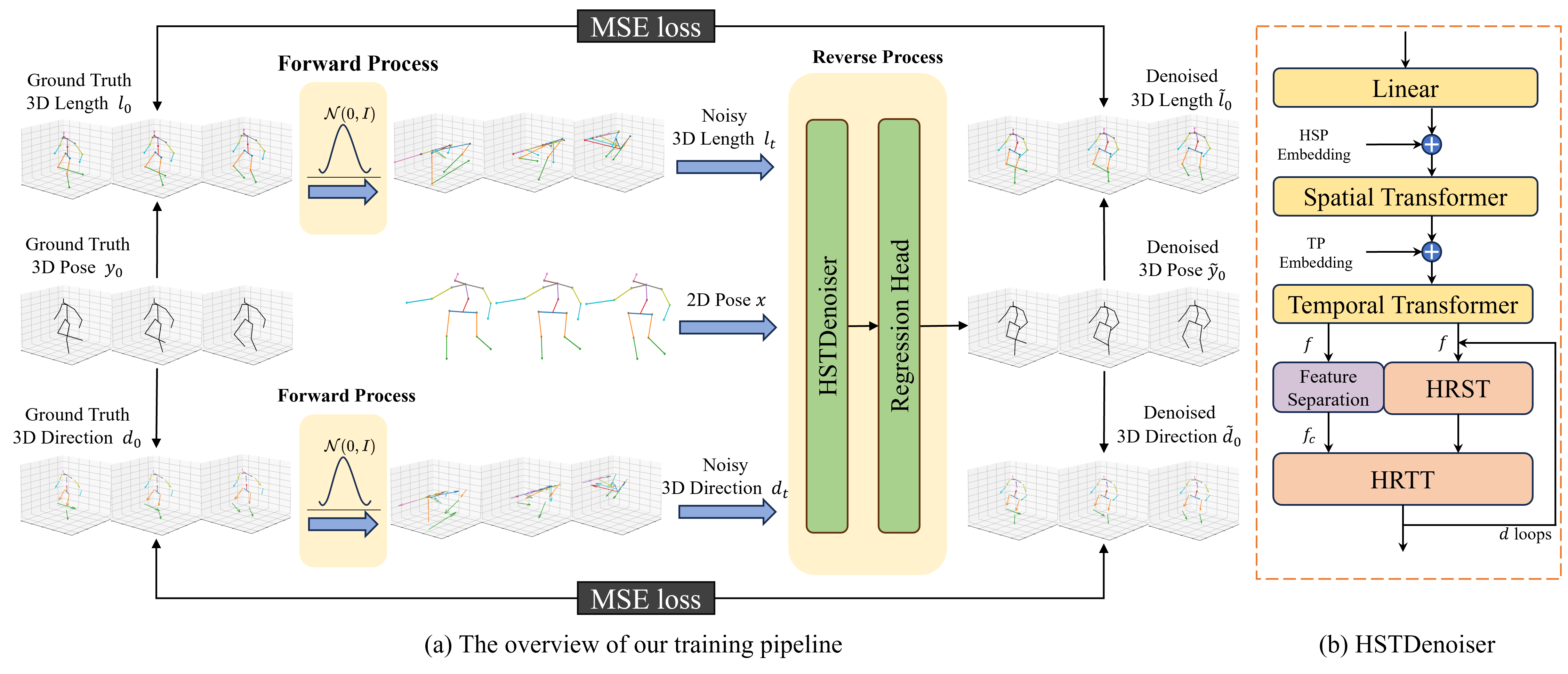
Figure 2: (a): The overview of DDHPose’s training pipeline. (b): The architecture of our HSTDenoiser, which contains HRST and HRTT. $HSP$ embedding and $TP$ embedding are used in the spatial-temporal transformer to better modeling the hierarchical relation of spatial position information and temporal position information. $f$ is the feature extracted by the spatial-temporal transformer and $f_{c}$ is the child joint feature separated from $f$. The input consists of $N$ frames for both 2D pose and 3D pose. For better clarity, only three frames of input are illustrated here as an example.

Recent explorations  (Choi, Shim, and Kim 2022; Holmquist and Wandt 2022; Ci et al. 2023; Shan et al. 2023) try to apply the diffusion model to 3D human pose estimation. Note that  (Gong et al. 2023) also uses a diffusion model for 3D HPE, but they additionally introduce the heatmap distribution of 2D pose, and the depth distribution to initialize 3D pose distribution, making a GMM-based forward diffusion process, so that they have a better performance than the other diffusion-based 3D HPE model. However, these approaches directly add $t$-step noise in the forward process to the original 3D pose, which is not conducive to learning the explicit human pose prior. Additionally,  (Xu et al. 2020; Chen et al. 2021; Wang et al. 2022) have a higher accumulation of errors that disentangle the 3D joint location to the prediction of bone length and bone direction. We introduce the disentanglement strategy in the forward process of the diffusion model, integrating the explicit human body prior to the diffusion model, and proposing the first disentangle-based diffusion model for 3D HPE. As a result, we achieve outstanding results on 3D HPE benchmarks.

Method

The overview of our proposed DDHPose is in Figure 2(a). In our framework, we decompose the 3D joint location into the bone length and bone direction, adding noise in the forward process. After the forward process, the noisy bone length, noisy bone direction, and 2D pose are fed to HSTDenoiser, which contains HRST and HRTT to reverse the 3D pose from the noisy input. Further details will be introduced in the following section.

3D POSE Disentanglement Strategy

We first introduce the motivation of why we use the disentanglement strategy in our paper. The original non-disentangle diffusion-based methods directly take the 3D joint sequence as input without any skeleton structural prior. Modeling the dependencies among each joint pair tends to be challenging due to their complex and dense relation which makes the optimization task more difficult. But in our approach, Our disentangle-based method first decomposes ground truth 3D pose $y_{0}\in\ \mathbb{R}^{N\times J\times 3}$ to bone length $l_{0}\in\ \mathbb{R}^{N\times(J-1)\times 1}$ and bone direction $d_{0}\in\ \mathbb{R}^{N\times(J-1)\times 3}$, where $N$ is the frame length of the input sequences, $J$ is the number of joints. This operation divides the dense and high-dimensional problem into multiple sparse and low-dimensional sub-problems, making the gradient-based optimization easier. Besides, The disentangling representation with bone length and direction makes it easier to add structural constraints, such as temporal consistency in bone length. The addition of bone length loss as a constraint enhances output certainty and shows effectiveness in the experiment.

For the $i$-th bone, ground truth length $l_{0}^{i}$ and direction $d_{0}^{i}$ can be defined as:

$$l_{0}^{i}=\left\|y_{0}^{c_{i}}-y_{0}^{p_{i}}\right\|_{2},\quad d_{0}^{i}=\frac{y_{0}^{c_{i}}-y_{0}^{p_{i}}}{\left\|y_{0}^{c_{i}}-y_{0}^{p_{i}}\right\|_{2}}$$ (1)

where $c_{i}$ and $p_{i}$ are the child joint and parent joint, which are in the upstream and downstream of the $i$-th bone according to the forward kinematic structure defined in the left portion of Figure 1.

The disentangled bone length and bone direction are both processed through the forward and reverse processes.

The Forward Process

The Forward Process is an approximate posterior that follows the Markov chain that gradually adds Gaussian noise $\mathcal{N}(0,I)$ to the original data $x_{0}$. Followed by DDPM (Ho, Jain, and Abbeel 2020), the forward process can be defined as:

$$q(x_{t}|x_{0}):=\mathcal{N}(x_{t};\sqrt{\bar{\alpha}_{t}}x_{0},(1-\bar{\alpha}_{t})I)\\$$ (2)

where $\bar{\alpha}_{t}:={\textstyle\prod_{s=0}^{t}}\alpha_{s}$ and $\alpha_{s}:=1-\beta_{s}$, $\beta_{s}$ is a noise schedule and we adopt the cosine-schedule proposed by  (Song and Ermon 2020) which always increases as the sampling step $t$ increases.

During the training stage in Figure 2(a), when we get the disentangled bone length $l_{0}$ and bone direction $d_{0}$, we can do the forward process separately in Eq (2) to get the noisy bone length $l_{t}$ and bone direction $d_{t}$ by adding $t$-step Gaussian noise as:

$$l_{t}=\sqrt{\bar{\alpha}_{t}}l_{0}+\sqrt{1-\bar{\alpha}_{t}}\epsilon,\quad d_{t}=\sqrt{\bar{\alpha}_{t}}d_{0}+\sqrt{1-\bar{\alpha}_{t}}\epsilon$$ (3)

where $\epsilon$ is the random Gaussian sampled at the $t$-step.

The Reverse Process

In the training stage, under the condition of a 2D pose sequence $x\in\ \mathbb{R}^{N\times J\times 2}$, the contaminated bone length $l_{t}$ and direction $d_{t}$ from the forward process are concatenated. This combined information is then processed through the HSTDenoiser and a regression head, resulting in the denoised 3D joints locations $\tilde{y}_{0}$. Then using our disentanglement strategy to decompose bone length $\tilde{l}_{0}$ and bone direction $\tilde{d}_{0}$ for disentanglement supervision during training.

At the inference stage, inspired by the method in D3DP (Shan et al. 2023), we simultaneously sample $H$ hypotheses from the Gaussian distribution as the initial noisy bone length and direction. They are then denoised through the trained denoiser, resulting in the denoised bone length $\tilde{l}_{0:H,0}$ and bone direction $\tilde{d}_{0:H,0}$. Then $\tilde{l}_{0:H,0}$ and $\tilde{l}_{0:H,0}$ are employed to generate noisy samples $\tilde{l}_{0:H,t^{\prime}}$ and $\tilde{d}_{0:H,t^{\prime}}$ in the next iteration at step $t^{\prime}$ via DDIM (Song, Meng, and Ermon 2020):

$$\begin{split}\tilde{l}_{0:H,t^{\prime}}&=\sqrt{\bar{\alpha}_{t^{\prime}}}\tilde{l}_{0:H,0}+\sqrt{1-\bar{\alpha}_{t^{\prime}}-\sigma_{t}^{2}}\cdot\epsilon_{tl}+\sigma_{t}\epsilon\\ \tilde{d}_{0:H,t^{\prime}}&=\sqrt{\bar{\alpha}_{t^{\prime}}}\tilde{d}_{0:H,0}+\sqrt{1-\bar{\alpha}_{t^{\prime}}-\sigma_{t}^{2}}\cdot\epsilon_{td}+\sigma_{t}\epsilon\end{split}$$ (4)

where $\epsilon_{tl}=\frac{\tilde{l}_{0:H,t}-\sqrt{\bar{\alpha}_{t}}\tilde{l}_{0:H,0}}{\sqrt{1-\bar{\alpha}_{t}}}$, $\epsilon_{td}=\frac{\tilde{d}_{0:H,t}-\sqrt{\bar{\alpha}_{t}}\tilde{d}_{0:H,0}}{\sqrt{1-\bar{\alpha}_{t}}}$ are the noise at step $t$ and $\sigma_{t}=\sqrt{(1-\bar{\alpha}_{t^{{}^{\prime}}})/(1-\bar{\alpha}_{t})}\cdot\sqrt{1-\bar{\alpha}_{t}/\bar{\alpha}_{t^{\prime}}}$ controls the stochastic of the diffusion process. We can control the hypothesis number $H$ and iteration times $W$ in the whole process. Appropriately increasing $H$ and $W$ can optimize the final prediction of the bone length and bone direction and improve the performance of MPJPE and P-MPJPE in our experiments.

Hierarchical Spatial and Temporal Denoiser

Both in the training or inference phase, noisy bone length and bone direction are fed into our HSTDenoiser to reconstruct the original data. HSTDenoiser, which consists of HRST and HRTT, is used to explore the hierarchical information, specifically the relation among the joint, the parent joint, and the child joint. The main architecture is shown in Figure 2(b). We utilize a linear layer to enhance the input feature and use the spatial-temporal transformer block in MixSTE (Zhang et al. 2022a) to extract joint features. We also introduce Hierarchical spatial position embedding $HSP$ for better spatial position modeling and temporal embedding $TP$ for better temporal position modeling. $HSP$ embedding not only contains the spatial position information of each joint but also contains the joint hierarchy information. Inspired by  (Li et al. 2023), we split the joints into six hierarchies according to the joint’s depth of the human body tree-like structure to build hierarchical embedding, which is shown in the left portion of Figure 1. It means the joints in the same hierarchy share the same embedding. Based on hierarchical embedding, the hierarchical-related information can be well learned by our model. After one layer of spatio-temporal transformer modeling, we utilize the HRST and HRTT, which we introduce in the subsequent section, to model the spatio-temporal correlations of joints through $d$ loops alternately.

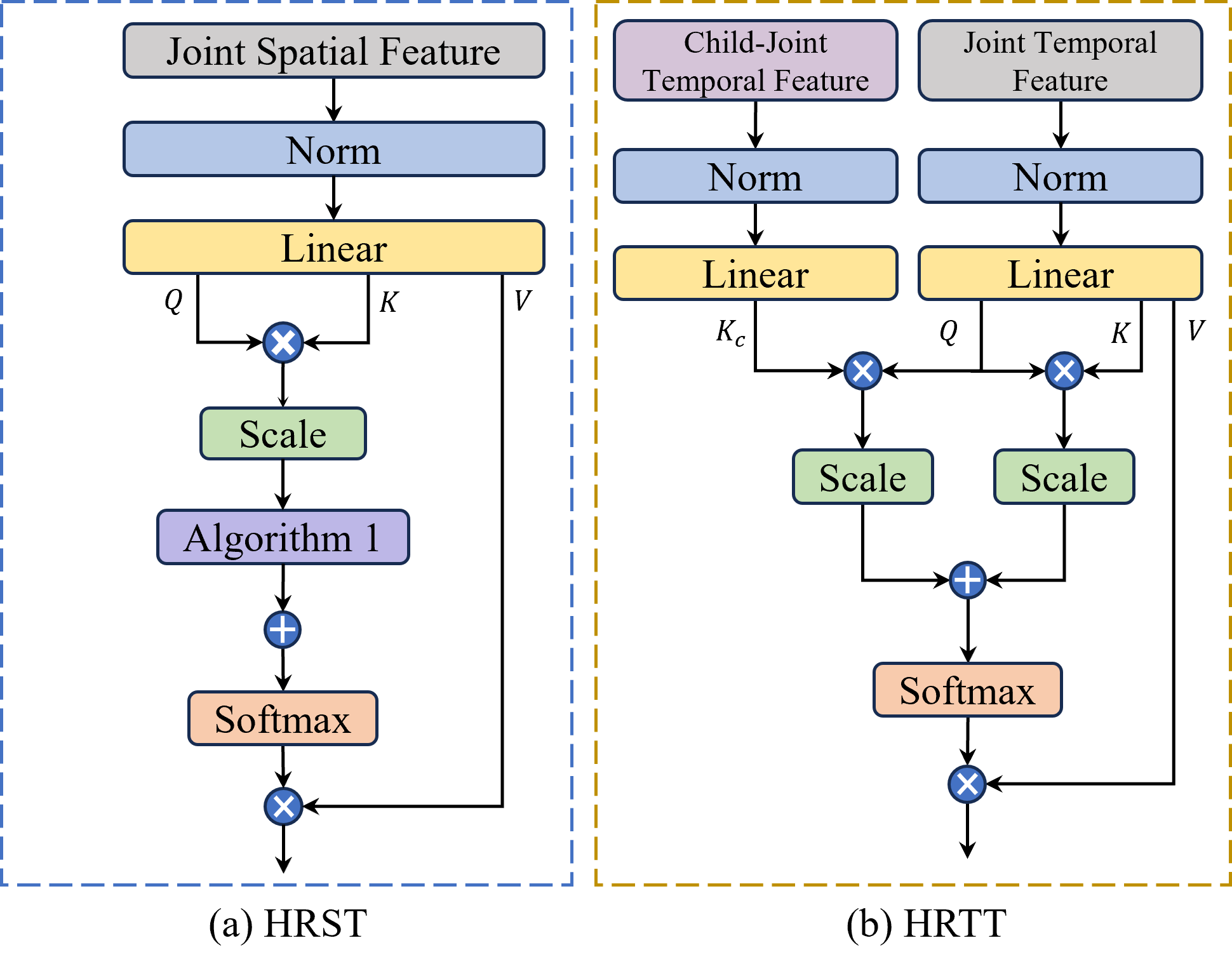
Figure 3: The main components of our HSTDenoiser. (a): Hierarchical-Related Spatial Transformer(HRST). (b): Hierarchical-Related Temporal Transformer(HRTT).

Transformer

The Transformer model we used in our approach is followed by  (Vaswani et al. 2017), the basic idea of query, key, and value is that the query is used to match with the key, and then according to the degree of matching, to selectively focus on the value. This design allows the output to selectively pay attention to the value based on the query. The mechanism of attention can be formulated by:

$$Attention=Softmax(A)V,\quad A=\frac{QK^{T}}{\sqrt{d_{m}}}$$ (5)

where ${Q,K,V}\in\mathbb{R}^{Z\times d_{m}}$ are generated by the input feature, $Z$ is the number of tokens and $d_{m}$ is the dimension of feature. $A\in\mathbb{R}^{Z\times Z}$ denotes the attention weight matrix.

The input of our transformer module is the noisy bone length and direction generated by the forward diffusion process. For better denoising, the 2D pose sequence is added as the condition and concatenated with the 3D noisy data as the whole input.

Algorithm 1 Hierarchical-Related Spatial Transformer

Input: $Q$, $K$, $V$ generated by Joint feature $f\in\mathbb{R}^{N\times J\times C}$
Parameter: Hierarchical Related joints triplets $\left\{J_{p},J,J_{c}\right\}$
Output:Hierarchical-Related spatial attention map

1:  $A=\frac{QK^{T}}{\sqrt{d_{m}}}$

2:  for $j_{p}$, $j$, $j_{c}$ in $J_{p}$, $J$, $J_{c}$ do

3:     $A$[$j$][$j_{c}$] += $A$[$j_{p}$][$j$]

4:     $A$[$j_{c}$][$j$] += $A$[$j_{p}$][$j$]

5:     $A$[$j$][$j_{c}$]/2.0 , $A$[$j_{c}$][$j$]/2.0

6:  end for

7:  return $A$

HRST

In HRST, we enhance the modeling of joint spatial information with its parent joint feature. Based on the forward kinematics structure, we define all the hierarchical-related joints triplets in the human body as $\left\{J_{p},J,J_{c}\right\}$, where $J_{p}$, $J$, $J_{c}$ are the set of $j_{p}$, $j$, $j_{c}$. In each of the hierarchical-related joints triplets $\left\{j_{p},j,j_{c}\right\}$, $j_{p}$ is the parent joint of joint $j$ and $j_{c}$ is the child joint of joint $j$ according to the forward kinematic structure. Because our method decomposes the location of joints into bone length and direction, we believe that the position of a joint is influenced by the position of its parent joint, combined with the bone length and direction. The attention of the parent joint significantly affects the attention of the joint. Therefore, in HRST, we augment the parent joint’s influence on each joint at the spatial level, specifically as illustrated in Algorithm 1. After Algorithm 1, we derive the weight matrix $A$ and then compute the attention utilizing Eq (5).

HRTT

We propose HRTT to further introduce the interrelationship between each joint and its hierarchical adjacent joints in the temporal dimension. In the process of exploring joint temporal information, we believe that due to the tree-like structure of the human skeleton, there exists a strong temporal correlation among a joint, its parent joint, and its child joints. Because we have enhanced the relation between a joint and its parent joint, the temporal relation between a joint and its child joints is more considered in HRTT.

Specifically, we primarily adopt a cross-attention mechanism to capture the relationship between the current joint and its child joints. According to the kinematic chain structure of human joints, we compute the average of its features with its child joints as the separated child joint feature $f_{c}$. We use a residual architecture to build the attention weight matrix. For detail, we use joint temporal feature $f$ after HRST to generate $Q$, $K$, $V$, formulating the self-attention weight matrix $A_{s}=\frac{QK^{T}}{\sqrt{d_{m}}}$. Concurrently, in the residual branch, we use the separated child joint feature $f_{c}$ to generate $K_{c}$, making cross-attention weight matrix with $Q$, which can be defined as $A_{c}=\frac{QK_{c}^{T}}{\sqrt{d_{m}}}$. Therefore, $A_{c}$ contains the cross-attention between a joint and its child joints in the temporal dimension. The shape of the temporal attention map $A_{s}$ and $A_{c}$ is $N\times N$, where $N$ is the frame length of the input sequences. $A_{s}$ and $A_{c}$ together dictate the temporal attention focused on $V$ as shown in Eq (6). Since $A_{s}$ contains the enhanced weight of both the joint and its parent joint feature, $A_{c}$ in the residual branch augments the relation between a joint and its child joints. Hence, HRTT effectively captures the relationships between the hierarchical adjacent joints.

$$\begin{split}Attention_{HRTT}&=Softmax(A_{s}+A_{c})V\\ \end{split}$$ (6)

Deterministic methods: Disentangle-based model
Protocol #1: MPJPE	Dir.	Disc.	Eat	Greet	Phone	Photo	Pose	Pur.	Sit	SitD.	Smoke	Wait	WalkD.	Walk	WalkT.	Avg.
DKA (Xu et al. 2020)($N$=9)	37.4	43.5	42.7	42.7	46.6	59.7	41.3	45.1	52.7	60.2	45.8	43.1	47.7	33.7	37.1	45.6
Anatomy3D (Chen et al. 2021)($N$=243)	41.4	43.5	40.1	42.9	46.6	51.9	41.7	42.3	53.9	60.2	45.4	41.7	46.0	31.5	32.7	44.1
Virtual Bones (Wang et al. 2022)($N$=243)	42.4	43.5	41.0	43.5	46.7	54.6	42.5	42.1	54.9	60.5	45.7	42.1	46.5	31.7	33.7	44.8
Ours ($N$=243, $H$=1, $W$=1)	37.3	40.0	35.2	37.7	41.1	46.7	38.4	38.4	52.2	53.3	41.4	38.9	38.8	27.6	27.7	39.7
Deterministic methods: Non-Disentangle based model
Protocol #1: MPJPE	Dir.	Disc.	Eat	Greet	Phone	Photo	Pose	Pur.	Sit	SitD.	Smoke	Wait	WalkD.	Walk	WalkT.	Avg.
VideoPose3D (Pavllo et al. 2019)($N$=243)	45.2	46.7	43.3	45.6	48.1	55.1	44.6	44.3	57.3	65.8	47.1	44.0	49.0	32.8	33.9	46.8
PoseFormer (Zheng et al. 2021)($N$=81)	41.5	44.8	39.8	42.5	46.5	51.6	42.1	42.0	53.3	60.7	45.5	43.3	46.1	31.8	32.2	44.3
P-STMO (Shan et al. 2022)($N$=243)	38.9	42.7	40.4	41.1	45.6	49.7	40.9	39.9	55.5	59.4	44.9	42.2	42.7	29.4	29.4	42.8
MixSTE (Zhang et al. 2022a)($N$=243)	37.6	40.9	37.3	39.7	42.3	49.9	40.1	39.8	51.7	55.0	42.1	39.8	41.0	27.9	27.9	40.9
PoseFormerV2 (Zhao et al. 2023)($N$=243)	41.3	45.5	41.5	44.0	46.7	53.8	42.6	42.6	55.2	64.6	45.7	42.9	45.8	32.3	32.9	45.2
STCFormer (Tang et al. 2023)($N$=243)	38.4	41.2	36.8	38.0	42.7	50.5	38.7	38.2	52.5	56.8	41.8	38.4	40.2	26.2	27.7	40.5
Ours ($N$=243, $H$=1, $W$=1)	37.3	40.0	35.2	37.7	41.1	46.7	38.4	38.4	52.2	53.3	41.4	38.9	38.8	27.6	27.7	39.7
Probabilistic methods
Protocol #1: MPJPE	Dir.	Disc.	Eat	Greet	Phone	Photo	Pose	Pur.	Sit	SitD.	Smoke	Wait	WalkD.	Walk	WalkT.	Avg.
MHFormer (Li et al. 2022b)($N$ =351, $H$=3)	39.2	43.1	40.1	40.9	44.9	51.2	40.6	41.3	53.5	60.3	43.7	41.1	43.8	29.8	30.6	43.0
GFPose (Ci et al. 2023)($H$ = 10)	39.9	44.6	40.2	41.3	46.7	53.6	41.9	40.4	52.1	67.1	45.7	42.9	46.1	36.5	38.0	45.1
D3DP (Shan et al. 2023)($N$=243,$*$)	37.3	39.5	35.6	37.8	41.3	48.2	39.1	37.6	49.9	52.8	41.2	39.2	39.4	27.2	27.1	39.5
Ours ($N$=243, $H$=5, $W$=1)	37.2	39.9	35.1	37.6	41.0	46.5	38.3	38.3	52.1	53.1	41.3	38.8	38.7	27.5	27.6	39.5
Ours ($N$=243, $H$=20, $W$=10)	36.4	39.5	34.9	37.6	40.1	45.9	37.8	37.8	51.5	52.2	40.8	38.3	38.3	27.0	27.0	39.0

Table 1: Results on Human3.6M in millimeters under MPJPE. $N$, $H$, $W$: the number of input frames, hypotheses, and iterations used in the inference stage. In this table, we compare with the deterministic and probabilistic methods. The best results are highlighted in bold. ($*$)-For clarity, $H$=20, $W$=10 is omitted.

Loss Function

3D Disentanglement Loss

3D disentanglement loss is utilized to aid the model in learning the explicit priors during the forward diffusion process. Given the 3D ground truth pose sequence $y_{0}$ and the predicted 3D pose sequence $\tilde{y}_{0}$ , we decompose $y_{0}$ to bone length $l_{0}$ and bone direction $d_{0}$. Similarly, we can obtain the disentangled bone length prediction $\tilde{l}_{0}$ and bone direction prediction $\tilde{d}_{0}$. And for the $i$-th bone, length $l_{0}^{i}$, $\tilde{l}_{0}^{i}$ and direction $d_{0}^{i}$, $\tilde{d}_{0}^{i}$ are defined as:

$$l_{0}^{i} =\left\|y_{0}^{c_{i}}-y_{0}^{p_{i}}\right\|_{2}, \tilde{l}_{0}^{i} =\left\|\tilde{y}_{0}^{c_{i}}-\tilde{y}_{0}^{p_{i}}\right\|_{2}$$ (7)

$$d_{0}^{i} =\frac{y_{0}^{c_{i}}-y_{0}^{p_{i}}}{\left\|y_{0}^{c_{i}}-y_{0}^{p_{i}}\right\|_{2}}, \tilde{d}_{0}^{i} =\frac{\tilde{y}_{0}^{c_{i}}-\tilde{y}_{0}^{p_{i}}}{\left\|\tilde{y}_{0}^{c_{i}}-\tilde{y}_{0}^{p_{i}}\right\|_{2}}$$

where $c_{i}$ and $p_{i}$ is the child joint and parent joint of the $i$-th bone. Then the disentanglement loss we use in our training stage can be defined as:

$$\begin{gathered}\begin{aligned} L_{l}&=\left\|\tilde{l}_{0}-l_{0}\right\|_{2},&L_{d}&=\left\|\tilde{d}_{0}-d_{0}\right\|_{2}\\ \end{aligned}\\ L_{dis}=L_{l}+L_{d}\end{gathered}$$ (8)

3D Pose Loss

During the model’s training process, we also use 3D pose loss to constrain the denoised 3D pose regressed by the model:

$$L_{pos}=\left\|\tilde{y}_{0}-y_{0}\right\|_{2}$$ (9)

By combining the 3D disentanglement loss and the 3D pose loss, the overall loss we used to supervise our model is given as:

$$L=L_{dis}+L_{pos}$$ (10)

Experiments

Dataset

Human3.6M

(Ionescu et al. 2014) is widely used in 3D HPE task. It contains 3.6 million 3D human poses and corresponding images with 11 professional actors and collected in 17 scenarios. Following the previous work  (Pavllo et al. 2019; Zheng et al. 2021; Zhang et al. 2022a), we use S1-S9 for training and use S9 and S11 for testing.

MPI-INF-3DHP

(Mehta et al. 2017) record 8 actors, composed of 4 males and 4 females, each undertaking 8 different sets of activities. We use eight activities performed by eight actors to train our model, while the test dataset has seven different activities.

Metrics

We use the mean per joint position error (MPJPE) and procrustes mean per joint position error(P-MPJPE) for evaluation. MPJPE measures the Euclidean distance between the ground truth and the predicted 3D positions of each joint while P-MPJPE makes procrustes analysis involves scaling, translating, and rotating the predicted pose to best align it with the ground truth, providing a more fair comparison. Following D3DP (Shan et al. 2023), we use J-AGG based MPJPE and P-MPJPE to evaluate our results.

Comparison with State-of-the-art Methods

Results on Human3.6M

The results of our method on Human3.6M are presented in Table 1. We first compare our method with the SOTA deterministic 3D human pose estimation methods. Based on whether the regression of the 3D pose locations is decomposed into the regression of bone length and bone direction, we divide the methods into disentangle-based methods and non-disentangle based methods. For disentangle-based methods, we can see from the table that our method achieves the best MPJPE of 39.7mm, surpassing Anatomy3D (Chen et al. 2021) by 4.4mm(10.0%) in MPJPE. For non-disentangle based model, we improve STCFormer (Tang et al. 2023) by 0.8mm(2.0%) under MPJPE. And then we compare our method with probabilistic methods, our method reaches the SOTA MPJPE of 39.0mm, outerperforms D3DP  (Shan et al. 2023) by 0.5mm(1.3%).

Method	MPJPE	P-MPJPE
DiffPose (Gong et al. 2023)($N$=243, $\flat$)	36.9	28.7
DiffPose$\sharp$ (Gong et al. 2023)($N$=243, $\flat$)	40.1	31.1
Ours ($N$=243, $H$=5, $W$=50)	39.2	31.1

Table 2: Comparison with DiffPose (Gong et al. 2023) on Human3.6M. ($\sharp$)- Stand-Diff implemented in DiffPose. ($\flat$)-For clarity, $H$=5, $W$=50 is omitted.

Method	PCK$\uparrow$	AUC$\uparrow$	MPJPE$\downarrow$
Anatomy3D (Chen et al. 2021)($N$=243)	87.8	53.8	79.1
PoseFormer (Zheng et al. 2021)($N$=9)	88.6	56.4	77.1
P-STMO (Shan et al. 2022)($N$=81)	97.9	75.8	32.2
MixSTE (Zhang et al. 2022a)($N$=243)	96.9	75.8	35.4
D3DP (Shan et al. 2023)($N$=243,$\natural$)	97.7	77.8	30.2
Ours ($N$=243,$\natural$)	98.5	78.1	29.2

Table 3: Results on MPI-INF-3DHP under PCK, AUC, and MPJPE using ground truth 2D pose as inputs. The best results are highlighted in bold. ($\natural$)-For clarity, $H$=1, $W$=1 is omitted.

As for DiffPose (Gong et al. 2023), we separately compare with it in Table 2. Note that, the DiffPose additionally introduces the heatmaps derived from an off-the-shelf 2D pose detector and depth distributions to initialize the pose distribution. The probabilistic methods in Table 1 only use the 2D pose sequences. Thus, it might not be fair to directly compare with DiffPose. But according to DiffPose, the implementation of Stand-Diff only uses 2D pose sequences by reversing the 3D pose from a standard Gaussian noise, which achieves a larger MPJPE error than our DDHPose with the same setting (40.1mm vs 39.2mm). The results demonstrate that our method can notably boost performance by 0.9mm through the Disentangle Strategy and the utilization of hierarchical relations.

Results on MPI-INF-3DHP

We also evaluate our method on the MPI-INF-3DHP dataset under PCK, AUC, and MPJPE metrics. In Table 3, our approach outperforms the SOTA method by 0.8 in PCK, 0.3 in AUC, and 1.0mm in MPJPE under the single hypothesis condition.

Disentangled Input	Disentangled Output	MPJPE	P-MPJPE
✗	✗	40.23	31.56
✗	✓	41.72	33.06
✓	✗	39.65	31.24
✓	✓	40.48	32.08

Table 4: The impact of disentanglement strategy. The disentanglement strategy with Disentangled input and without Disentangled output has the best result highlighted in bold.

Ablation Study

In order to evaluate each design in our method, we conduct ablation experiments on the Human3.6M dataset using 2D pose sequence extracted by CPN.

Impact of Disentanglement Strategy

In this section, we separately compare the effect of the Disentangle Input and Disentangle Output strategy.

For the Disentangle Input Strategy, our method divides the dense and high-dimensional optimization problem into two low-dimensional sub-problems, simplifying the learning of the human pose prior. As shown in the left portion of Figure 4, employing the Disentangle Input strategy results in faster convergence and lower training 3D pose loss compared to not using it in the initial training epoch. This leads to improved quantitative results (39.65mm vs 40.23mm), as highlighted in Table 4.

For Disentangle Output, the denoiser in the reverse process directly regresses bone length and direction, generating the 3D pose using $C=C_{p}+l\times d$, where $C$ and $C_{p}$ are joint and parent joint coordinates, and $l$, $d$ represent predicted bone length and direction. This equation indicates that a joint’s coordinate depends not only on its own bone properties but also on all parent joints along the bone chain. As illustrated in the right portion of Figure 4, hierarchy 1 exhibits lower errors in the Disentangled Output setting, while higher hierarchical levels accumulate errors more than without using Disentangled Output. Quantitative results in Table 4 show that employing the Disentangle Output strategy increases MPJPE from 40.23mm to 41.72mm.

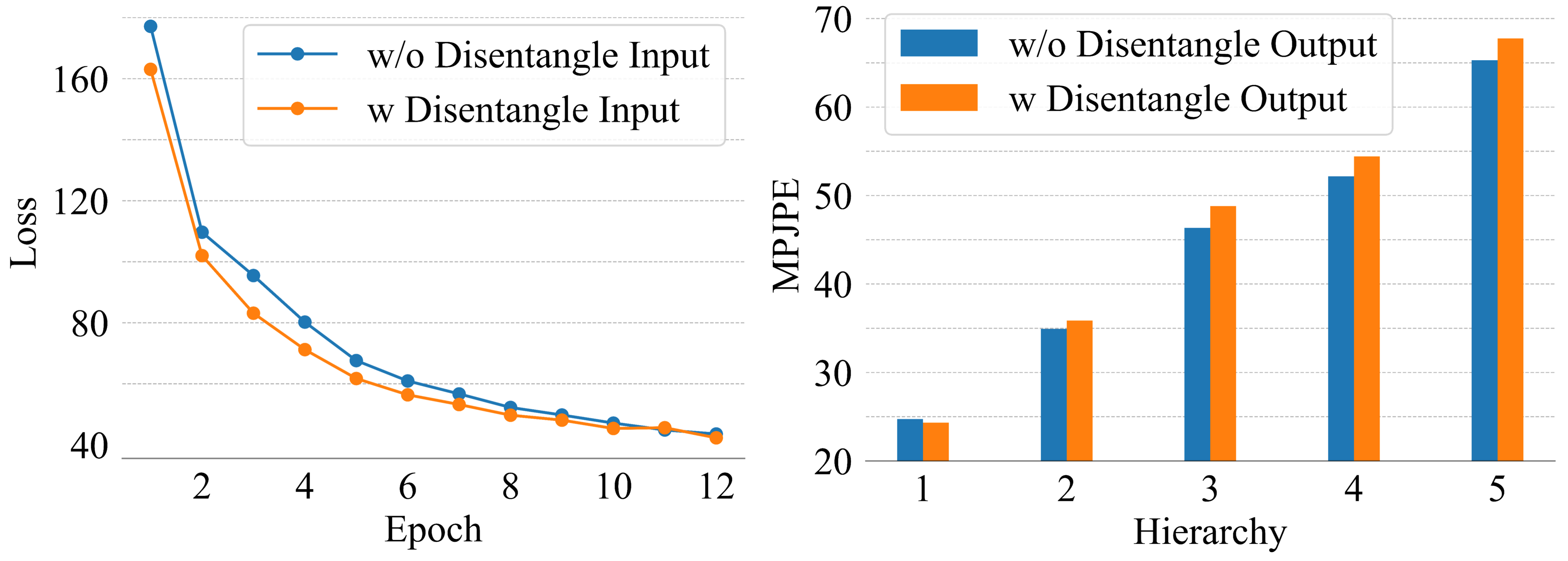
Figure 4: Left: Training Loss Comparison (w/o Disentangle Output). Right: Hierarchical Error Comparison (w/o Disentangle Input).

Effect of each module

As shown in Table 5. We can divide our method into three modules: Hierarchical embedding, HRST, and HRTT. In our experiment, we sequentially add the modules to the baseline, which doesn’t use any of the three modules to verify the effectiveness of each module. For simplicity, we set both $H$ and $W$ to 1.

baseline	Hierarchical embedding	HRST	HRTT	MPJPE	P-MPJPE
✓				40.10	31.94
✓	✓			40.08	31.83
✓	✓	✓		39.68	31.55
✓	✓	✓	✓	39.65	31.24

Table 5: Effect of each module in our experiments on Human3.6M dataset. The best results are highlighted in bold.

The result shows that hierarchical embedding provides a slight improvement over the baseline. Adding HRST can boost MPJPE from 40.08mm to 39.68mm and lifts P-MPJPE from 31.83mm to 31.55mm. Further integrating HRTT refines the MPJPE from 39.68mm to 39.65mm and boosts P-MPJPE from 31.55mm to 31.24mm. The results suggest that information from the parent joint influences the regression of the joint itself, which assists the model in learning the joint’s spatial information. The shared information between parent and child joints aids the model in inferring the temporal feature of the joint.

Effect of Loss Function

We employ the 3D pose loss to constrain the denoised 3D pose regressed by our model and utilize the 3D disentanglement loss to aid the model in learning the explicit human body prior during the forward diffusion process. The contribution of the loss function is in Table 6. The result shows that using 3D disentanglement loss is essential for a better result. With the 3D disentanglement loss, the performance of MPJPE and P-MPJPE can be improved by 0.22mm and 0.70mm.

	MPJPE	P-MPJPE
3D pos loss	39.87	31.94
3D pos loss + 3D dis loss	39.65	31.24

Table 6: Ablation study for loss function proposed in our method. The best results are highlighted in bold.

Conclusion

In this paper, we propose DDHPose, a diffusion-based 3D HPE method that introduces hierarchical information in two ways: (1)We propose the Disentangle Strategy for the forward diffusion process, which decomposes the 3D pose into bone length and direction based on the Hierarchical Information. This simplifies learning the human pose prior, reduces optimization dimension, and speeds up gradient descent. (2)We propose HSTDenoiser to strengthen the relation among the hierarchical joints by enhancing the attention weight of adjacent joints for each joint in the reverse diffusion process. Extensive results on Human3.6M and MPI-INF-3DHP reveal that our method surpasses the disentangle-based method, non-disentangle based method, and the probabilistic approaches on 3D HPE benchmarks.

Appendix

Deterministic methods: Disentangle-based model
Protocol #2: P-MPJPE	Dir.	Disc.	Eat	Greet	Phone	Photo	Pose	Pur.	Sit	SitD.	Smoke	Wait	WalkD.	Walk	WalkT.	Avg.
DKA (Xu et al. 2020)($N$=9)	31.0	34.8	34.7	34.4	36.2	43.9	31.6	33.5	42.3	49.0	37.1	33.0	39.1	26.9	31.9	36.2
Anatomy3D (Chen et al. 2021)($N$=243)	32.6	35.1	32.8	35.4	36.3	40.4	32.4	32.3	42.7	49.0	36.8	32.4	36.0	24.9	26.5	35.0
Virtual Bones (Wang et al. 2022)($N$=243)	32.2	34.9	33.0	35.2	35.7	40.7	32.6	32.1	42.8	48.9	36.5	32.5	35.9	25.0	26.7	34.9
Ours($N$=243, $H$=1, $W$=1)	29.5	31.9	28.7	30.1	31.3	35.5	29.7	29.5	41.8	42.9	33.4	29.7	30.4	21.7	22.6	31.2
Deterministic methods: Non-Disentangle-based model
Protocol #2: P-MPJPE	Dir.	Disc.	Eat	Greet	Phone	Photo	Pose	Pur.	Sit	SitD.	Smoke	Wait	WalkD.	Walk	WalkT.	Avg.
VideoPose3D (Pavllo et al. 2019)($N$=243)	34.1	36.1	34.4	37.2	36.4	42.2	34.4	33.6	45.0	52.5	37.4	33.8	37.8	25.6	27.3	36.5
PoseFormer (Zheng et al. 2021)($N$=81)	34.1	36.1	34.4	37.2	34.4	39.2	32.0	31.8	42.9	46.9	35.5	32.0	34.4	23.6	25.2	33.9
P-STMO (Shan et al. 2022)($N$ =243)	31.3	35.2	32.9	33.9	35.4	39.3	32.5	31.5	44.6	48.2	36.3	32.9	34.4	23.8	23.9	34.4
MixSTE (Zhang et al. 2022a)($N$ =243)	30.8	33.1	30.3	31.8	33.1	39.1	31.1	30.5	42.5	44.5	34.0	30.8	32.7	22.1	22.9	32.6
PoseFormerV2 (Zhao et al. 2023)($N$ =243)	32.3	35.9	33.8	35.8	36.0	41.1	33.2	32.7	44.3	51.9	37.4	32.8	35.6	25.2	26.6	35.6
STCFormer (Tang et al. 2023)($N$=243)	29.3	33.0	30.7	30.6	32.7	38.2	29.7	28.8	42.2	45.0	33.3	29.4	31.5	20.9	22.3	31.8
Ours($N$=243, $H$=1, $W$=1)	29.5	31.9	28.7	30.1	31.3	35.5	29.7	29.5	41.8	42.9	33.4	29.7	30.4	21.7	22.6	31.2
Probabilistic methods
Protocol #2: P-MPJPE	Dir.	Disc.	Eat	Greet	Phone	Photo	Pose	Pur.	Sit	SitD.	Smoke	Wait	WalkD.	Walk	WalkT.	Avg.
MHFormer (Li et al. 2022b)($N$=351,$H$=3)	31.5	34.9	32.8	33.6	35.3	39.6	32.0	32.2	43.5	48.7	36.4	32.6	34.3	23.9	25.1	34.4
GFPose (Ci et al. 2023)($H$ = 10)	32.0	39.5	34.4	34.7	38.6	44.3	32.7	31.9	49.0	60.1	38.9	36.6	42.2	28.3	32.3	38.4
D3DP (Shan et al. 2023)($N$=243, $*$)	30.6	32.4	29.2	30.9	31.9	37.4	30.2	29.3	40.4	43.2	33.2	30.4	31.3	21.5	22.3	31.6
Ours($N$=243,$H$=5, $W$=1)	29.5	31.8	28.7	30.1	31.3	35.6	29.7	29.5	41.7	42.9	33.4	29.6	30.4	21.7	22.6	31.2
Ours($N$=243, $H$=20, $W$=10)	29.4	32.1	28.4	30.1	31.0	35.3	29.5	29.2	41.7	42.7	33.2	29.7	30.6	21.5	22.2	31.2

Table 7: Results on Human3.6M in millimeters under P-MPJPE. $N$, $H$, $W$: the number of input frames, hypotheses, and iterations used in the inference stage. In this table, we are compared with the deterministic and probabilistic methods. The best results are highlighted in bold. ($*$)-For clarity, $H$=20, $W$=10 is omitted.

Implementation Details

Our model is implemented in Pytorch  (Paszke et al. 2019), using AdamW  (Loshchilov and Hutter 2017) as our optimizer with the momentum parameters as $\beta_{1}$, $\beta_{2}$ = 0.9, 0.999. We train our model for 400 epochs on NVIDIA Tesla A800 and the initial learning rate is 1$e^{-4}$, with a shrink factor of 0.993. We set batch size to 4 and in each batch, we use the length of 243 frames to train our model. We use a total of eight layers of spatio-temporal transformers in our model. The timestep $t$ is sampled from $U(0,\mathcal{T})$ during training, where $\mathcal{T}$ is the maximum number of timesteps and is set to 1000. The first layer employed the spatio-temporal transformer in MixSTE  (Zhang et al. 2022a), followed by seven layers of HRST and HRTT used in a loop.

Inference Details

During the inference stage, we simultaneously sample $H$ bone length and bone direction hypotheses from a standard normal Gaussian distribution $\mathcal{N}(0,I)$ at the initial timestep $\mathcal{T}$ for the diffusion-based HSTDenoiser. The noisy 3D bone length $l_{0:H,\mathcal{T}}$ and bone direction $d_{0:H,\mathcal{T}}$, with the condition of the 2D pose sequence, are denoised by our denoiser and make predictions of 3D poses $\tilde{y}_{0:H,0}$. Then we can decompose $\tilde{y}_{0:H,0}$ to get the feasible predictions of bone length $\tilde{l}_{0:H,0}$ and bone direction $\tilde{d}_{0:H,0}$.

The denoised $\tilde{l}_{0:H,0}$ and $\tilde{d}_{0:H,0}$ can be used to generate the noisy input $l_{0:H,t^{{}^{\prime}}}$ and $d_{0:H,t^{{}^{\prime}}}$ at timestep $t^{{}^{\prime}}$ via DDIM(Song, Meng, and Ermon 2020), which is formulated in Eq (4) and shown in Figure 5. The updated input $l_{0:H,t^{{}^{\prime}}}$ and $d_{0:H,t^{{}^{\prime}}}$ will lead to another refined prediction and this procedure can be repeated for $W$ times to get the final predictions, which can enhance the prediction performance to some extent.

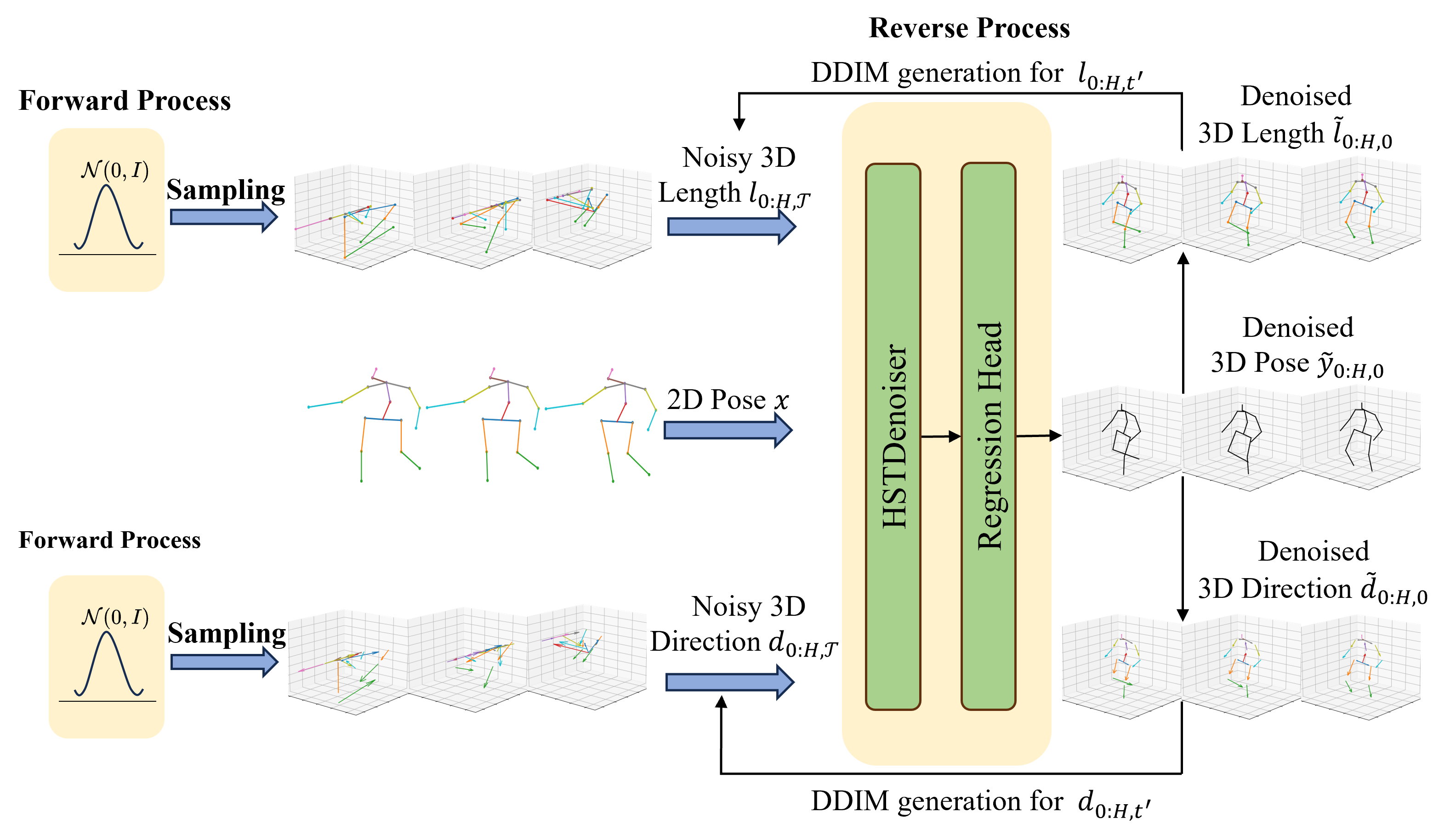
Figure 5: The overview of the inference pipeline.

Additional Quantitative Results

The supplement comparison of P-MPJPE is shown in Table 7. We compare our method with the SOTA deterministic methods and probabilistic methods. Based on whether the regression of the 3D pose locations is decomposed into the regression of bone length and bone direction, we divide the methods into disentangle-based methods and non-disentangle based methods. For disentangle-based methods, we can see from the table that our method achieves the best P-MPJPE of 31.2mm, which outperforms Anatomy3D (Chen et al. 2021) by 3.7mm(10.6%). While for non-disentangle based model, we improve STCFormer (Tang et al. 2023) by 0.6mm(1.9%) under P-MPJPE. And then we compare our method with probabilistic methods, our method reaches the SOTA MPJPE of 31.2mm, outerperforms D3DP  (Shan et al. 2023) by 0.4mm(1.3%).

Qualitative results

We evaluate the qualitative results between our method, MixSTE (Zhang et al. 2022a) and D3DP (Shan et al. 2023). The visual results are in Figure 6. Our method has better results than MixSTE and D3DP for the high hierarchical joints where the black dashed circle highlighting in the figure.

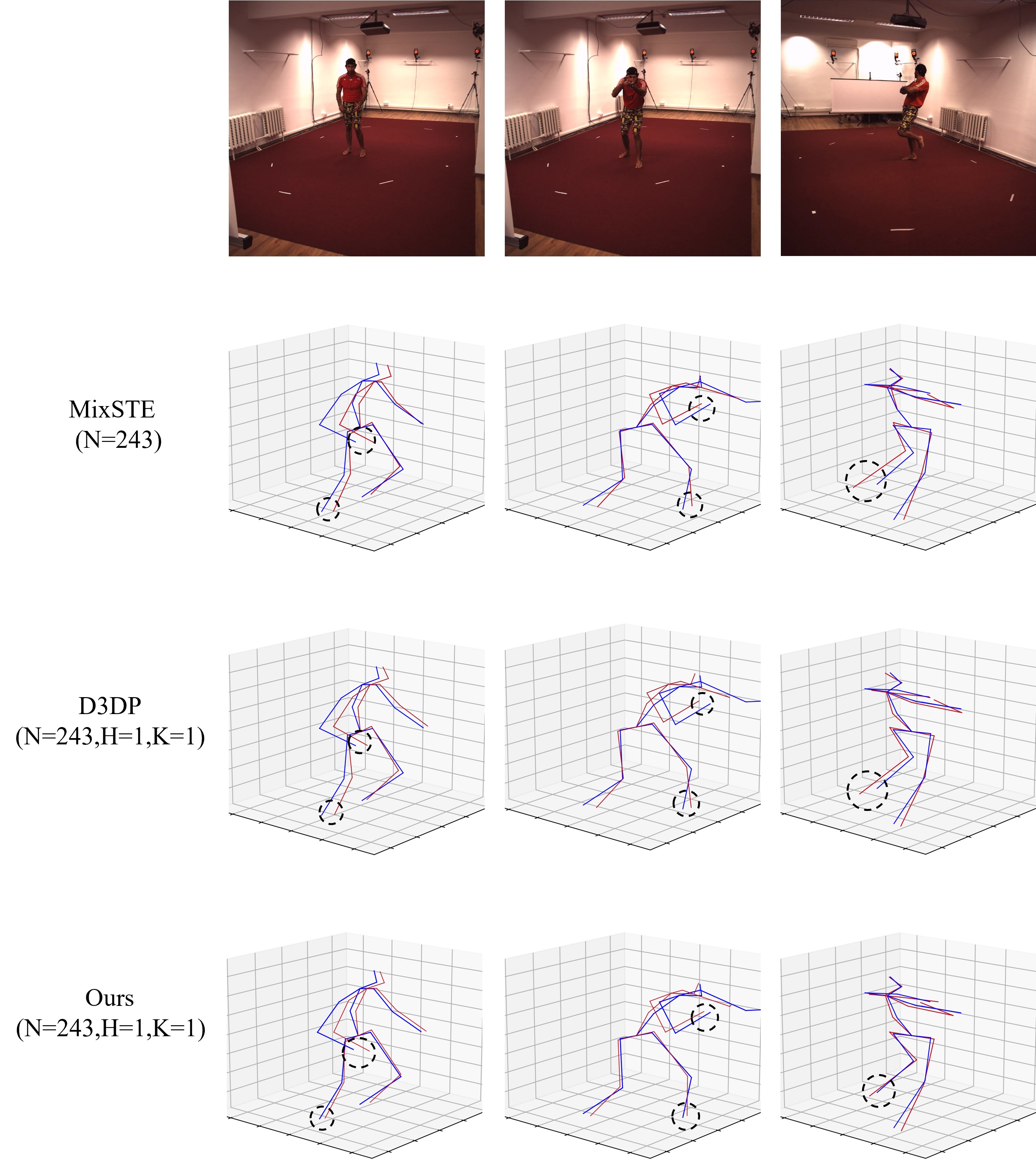
Figure 6: Qualitative comparison between our method, MixSTE and D3DP on Human3.6M. The ground truth pose is drawn in blue and the predicted pose is drawn in red. The black dashed circle highlights the locations where our method has better results.

References

- Baranchuk et al. (2021) Baranchuk, D.; Rubachev, I.; Voynov, A.; Khrulkov, V.; and Babenko, A. 2021. Label-efficient semantic segmentation with diffusion models. arXiv preprint arXiv:2112.03126.
- Batzolis et al. (2021) Batzolis, G.; Stanczuk, J.; Schönlieb, C.-B.; and Etmann, C. 2021. Conditional image generation with score-based diffusion models. arXiv preprint arXiv:2111.13606.
- Cao et al. (2017) Cao, Z.; Simon, T.; Wei, S.-E.; and Sheikh, Y. 2017. Realtime Multi-Person 2D Pose Estimation using Part Affinity Fields. In CVPR.
- Chen et al. (2021) Chen, T.; Fang, C.; Shen, X.; Zhu, Y.; Chen, Z.; and Luo, J. 2021. Anatomy-aware 3d human pose estimation with bone-based pose decomposition. IEEE Transactions on Circuits and Systems for Video Technology, 32(1): 198–209.
- Chen et al. (2018) Chen, Y.; Wang, Z.; Peng, Y.; Zhang, Z.; Yu, G.; and Sun, J. 2018. Cascaded pyramid network for multi-person pose estimation. In Proceedings of the IEEE conference on computer vision and pattern recognition, 7103–7112.
- Choi, Shim, and Kim (2022) Choi, J.; Shim, D.; and Kim, H. J. 2022. Diffupose: Monocular 3d human pose estimation via denoising diffusion probabilistic model. arXiv preprint arXiv:2212.02796.
- Ci et al. (2023) Ci, H.; Wu, M.; Zhu, W.; Ma, X.; Dong, H.; Zhong, F.; and Wang, Y. 2023. Gfpose: Learning 3d human pose prior with gradient fields. In Proceedings of the IEEE/CVF Conference on Computer Vision and Pattern Recognition, 4800–4810.
- Dinh, Krueger, and Bengio (2014) Dinh, L.; Krueger, D.; and Bengio, Y. 2014. Nice: Non-linear independent components estimation. arXiv preprint arXiv:1410.8516.
- Dinh, Sohl-Dickstein, and Bengio (2016) Dinh, L.; Sohl-Dickstein, J.; and Bengio, S. 2016. Density estimation using real nvp. arXiv preprint arXiv:1605.08803.
- Fan et al. (2023) Fan, W.-C.; Chen, Y.-C.; Chen, D.; Cheng, Y.; Yuan, L.; and Wang, Y.-C. F. 2023. Frido: Feature pyramid diffusion for complex scene image synthesis. In Proceedings of the AAAI Conference on Artificial Intelligence, volume 37, 579–587.
- Fang et al. (2017) Fang, H.-S.; Xie, S.; Tai, Y.-W.; and Lu, C. 2017. RMPE: Regional Multi-person Pose Estimation. In ICCV.
- Gong et al. (2023) Gong, J.; Foo, L. G.; Fan, Z.; Ke, Q.; Rahmani, H.; and Liu, J. 2023. Diffpose: Toward more reliable 3d pose estimation. In Proceedings of the IEEE/CVF Conference on Computer Vision and Pattern Recognition, 13041–13051.
- Goodfellow et al. (2020) Goodfellow, I.; Pouget-Abadie, J.; Mirza, M.; Xu, B.; Warde-Farley, D.; Ozair, S.; Courville, A.; and Bengio, Y. 2020. Generative adversarial networks. Communications of the ACM, 63(11): 139–144.
- Hagbi et al. (2010) Hagbi, N.; Bergig, O.; El-Sana, J.; and Billinghurst, M. 2010. Shape recognition and pose estimation for mobile augmented reality. IEEE transactions on visualization and computer graphics, 17(10): 1369–1379.
- Ho, Jain, and Abbeel (2020) Ho, J.; Jain, A.; and Abbeel, P. 2020. Denoising diffusion probabilistic models. Advances in neural information processing systems, 33: 6840–6851.
- Ho et al. (2022) Ho, J.; Saharia, C.; Chan, W.; Fleet, D. J.; Norouzi, M.; and Salimans, T. 2022. Cascaded diffusion models for high fidelity image generation. The Journal of Machine Learning Research, 23(1): 2249–2281.
- Holmquist and Wandt (2022) Holmquist, K.; and Wandt, B. 2022. Diffpose: Multi-hypothesis human pose estimation using diffusion models. arXiv preprint arXiv:2211.16487.
- Hyvärinen and Dayan (2005) Hyvärinen, A.; and Dayan, P. 2005. Estimation of non-normalized statistical models by score matching. Journal of Machine Learning Research, 6(4).
- Ionescu et al. (2014) Ionescu, C.; Papava, D.; Olaru, V.; and Sminchisescu, C. 2014. Human3.6M: Large Scale Datasets and Predictive Methods for 3D Human Sensing in Natural Environments. IEEE Transactions on Pattern Analysis and Machine Intelligence, 36(7): 1325–1339.
- Kingma and Dhariwal (2018) Kingma, D. P.; and Dhariwal, P. 2018. Glow: Generative flow with invertible 1x1 convolutions. Advances in neural information processing systems, 31.
- Kingma and Welling (2013) Kingma, D. P.; and Welling, M. 2013. Auto-encoding variational bayes. arXiv preprint arXiv:1312.6114.
- Kisacanin, Pavlovic, and Huang (2005) Kisacanin, B.; Pavlovic, V.; and Huang, T. S. 2005. Real-time vision for human-computer interaction. Springer Science & Business Media.
- Li et al. (2023) Li, H.; Shi, B.; Dai, W.; Zheng, H.; Wang, B.; Sun, Y.; Guo, M.; Li, C.; Zou, J.; and Xiong, H. 2023. Pose-Oriented Transformer with Uncertainty-Guided Refinement for 2D-to-3D Human Pose Estimation. In Proceedings of the AAAI Conference on Artificial Intelligence, volume 37, 1296–1304.
- Li et al. (2022a) Li, W.; Liu, H.; Ding, R.; Liu, M.; Wang, P.; and Yang, W. 2022a. Exploiting temporal contexts with strided transformer for 3d human pose estimation. IEEE Transactions on Multimedia, 25: 1282–1293.
- Li et al. (2022b) Li, W.; Liu, H.; Tang, H.; Wang, P.; and Van Gool, L. 2022b. Mhformer: Multi-hypothesis transformer for 3d human pose estimation. In Proceedings of the IEEE/CVF Conference on Computer Vision and Pattern Recognition, 13147–13156.
- Loshchilov and Hutter (2017) Loshchilov, I.; and Hutter, F. 2017. Decoupled weight decay regularization. arXiv preprint arXiv:1711.05101.
- Mehta et al. (2017) Mehta, D.; Rhodin, H.; Casas, D.; Fua, P.; Sotnychenko, O.; Xu, W.; and Theobalt, C. 2017. Monocular 3D Human Pose Estimation In The Wild Using Improved CNN Supervision. In 3D Vision (3DV), 2017 Fifth International Conference on. IEEE.
- Nichol et al. (2021) Nichol, A.; Dhariwal, P.; Ramesh, A.; Shyam, P.; Mishkin, P.; McGrew, B.; Sutskever, I.; and Chen, M. 2021. Glide: Towards photorealistic image generation and editing with text-guided diffusion models. arXiv preprint arXiv:2112.10741.
- Nichol and Dhariwal (2021) Nichol, A. Q.; and Dhariwal, P. 2021. Improved denoising diffusion probabilistic models. In International Conference on Machine Learning, 8162–8171. PMLR.
- Paszke et al. (2019) Paszke, A.; Gross, S.; Massa, F.; Lerer, A.; Bradbury, J.; Chanan, G.; Killeen, T.; Lin, Z.; Gimelshein, N.; Antiga, L.; et al. 2019. Pytorch: An imperative style, high-performance deep learning library. Advances in neural information processing systems, 32.
- Pavlakos et al. (2017) Pavlakos, G.; Zhou, X.; Derpanis, K. G.; and Daniilidis, K. 2017. Coarse-to-fine volumetric prediction for single-image 3D human pose. In Proceedings of the IEEE conference on computer vision and pattern recognition, 7025–7034.
- Pavllo et al. (2019) Pavllo, D.; Feichtenhofer, C.; Grangier, D.; and Auli, M. 2019. 3D human pose estimation in video with temporal convolutions and semi-supervised training. In Conference on Computer Vision and Pattern Recognition (CVPR).
- Qian et al. (2023) Qian, X.; Tang, Y.; Zhang, N.; Han, M.; Xiao, J.; Huang, M.-C.; and Lin, R.-S. 2023. HSTFormer: Hierarchical Spatial-Temporal Transformers for 3D Human Pose Estimation. arXiv preprint arXiv:2301.07322.
- Saharia et al. (2022) Saharia, C.; Ho, J.; Chan, W.; Salimans, T.; Fleet, D. J.; and Norouzi, M. 2022. Image super-resolution via iterative refinement. IEEE Transactions on Pattern Analysis and Machine Intelligence, 45(4): 4713–4726.
- Shan et al. (2022) Shan, W.; Liu, Z.; Zhang, X.; Wang, S.; Ma, S.; and Gao, W. 2022. P-stmo: Pre-trained spatial temporal many-to-one model for 3d human pose estimation. In European Conference on Computer Vision, 461–478. Springer.
- Shan et al. (2023) Shan, W.; Liu, Z.; Zhang, X.; Wang, Z.; Han, K.; Wang, S.; Ma, S.; and Gao, W. 2023. Diffusion-Based 3D Human Pose Estimation with Multi-Hypothesis Aggregation. arXiv preprint arXiv:2303.11579.
- Sohl-Dickstein et al. (2015) Sohl-Dickstein, J.; Weiss, E.; Maheswaranathan, N.; and Ganguli, S. 2015. Deep unsupervised learning using nonequilibrium thermodynamics. In International conference on machine learning, 2256–2265. PMLR.
- Song, Meng, and Ermon (2020) Song, J.; Meng, C.; and Ermon, S. 2020. Denoising diffusion implicit models. arXiv preprint arXiv:2010.02502.
- Song et al. (2021) Song, Y.; Durkan, C.; Murray, I.; and Ermon, S. 2021. Maximum likelihood training of score-based diffusion models. Advances in Neural Information Processing Systems, 34: 1415–1428.
- Song and Ermon (2019) Song, Y.; and Ermon, S. 2019. Generative modeling by estimating gradients of the data distribution. Advances in neural information processing systems, 32.
- Song and Ermon (2020) Song, Y.; and Ermon, S. 2020. Improved techniques for training score-based generative models. Advances in neural information processing systems, 33: 12438–12448.
- Song et al. (2020) Song, Y.; Garg, S.; Shi, J.; and Ermon, S. 2020. Sliced score matching: A scalable approach to density and score estimation. In Uncertainty in Artificial Intelligence, 574–584. PMLR.
- Sun et al. (2018) Sun, X.; Xiao, B.; Wei, F.; Liang, S.; and Wei, Y. 2018. Integral human pose regression. In Proceedings of the European conference on computer vision (ECCV), 529–545.
- Tang et al. (2023) Tang, Z.; Qiu, Z.; Hao, Y.; Hong, R.; and Yao, T. 2023. 3D Human Pose Estimation With Spatio-Temporal Criss-Cross Attention. In Proceedings of the IEEE/CVF Conference on Computer Vision and Pattern Recognition, 4790–4799.
- Tekin et al. (2016) Tekin, B.; Rozantsev, A.; Lepetit, V.; and Fua, P. 2016. Direct prediction of 3d body poses from motion compensated sequences. In Proceedings of the IEEE Conference on Computer Vision and Pattern Recognition, 991–1000.
- Vaswani et al. (2017) Vaswani, A.; Shazeer, N.; Parmar, N.; Uszkoreit, J.; Jones, L.; Gomez, A.; Kaiser, L.; and Polosukhin, I. 2017. Attention is All you Need. Neural Information Processing Systems,Neural Information Processing Systems.
- Vincent (2011) Vincent, P. 2011. A connection between score matching and denoising autoencoders. Neural computation, 23(7): 1661–1674.
- Wang et al. (2022) Wang, G.; Zeng, H.; Wang, Z.; Liu, Z.; and Wang, H. 2022. Motion Projection Consistency Based 3D Human Pose Estimation with Virtual Bones from Monocular Videos. IEEE Transactions on Cognitive and Developmental Systems.
- Wang et al. (2020) Wang, J.; Sun, K.; Cheng, T.; Jiang, B.; Deng, C.; Zhao, Y.; Liu, D.; Mu, Y.; Tan, M.; Wang, X.; et al. 2020. Deep high-resolution representation learning for visual recognition. IEEE transactions on pattern analysis and machine intelligence, 43(10): 3349–3364.
- Xu et al. (2020) Xu, J.; Yu, Z.; Ni, B.; Yang, J.; Yang, X.; and Zhang, W. 2020. Deep kinematics analysis for monocular 3d human pose estimation. In Proceedings of the IEEE/CVF Conference on computer vision and Pattern recognition, 899–908.
- Zhang et al. (2022a) Zhang, J.; Tu, Z.; Yang, J.; Chen, Y.; and Yuan, J. 2022a. MixSTE: Seq2seq Mixed Spatio-Temporal Encoder for 3D Human Pose Estimation in Video. In Proceedings of the IEEE/CVF Conference on Computer Vision and Pattern Recognition (CVPR), 13232–13242.
- Zhang et al. (2022b) Zhang, J.; Ye, G.; Tu, Z.; Qin, Y.; Qin, Q.; Zhang, J.; and Liu, J. 2022b. A spatial attentive and temporal dilated (SATD) GCN for skeleton-based action recognition. CAAI Transactions on Intelligence Technology, 7(1): 46–55.
- Zhao et al. (2023) Zhao, Q.; Zheng, C.; Liu, M.; Wang, P.; and Chen, C. 2023. PoseFormerV2: Exploring Frequency Domain for Efficient and Robust 3D Human Pose Estimation. In Proceedings of the IEEE/CVF Conference on Computer Vision and Pattern Recognition (CVPR), 8877–8886.
- Zheng et al. (2021) Zheng, C.; Zhu, S.; Mendieta, M.; Yang, T.; Chen, C.; and Ding, Z. 2021. 3d human pose estimation with spatial and temporal transformers. In Proceedings of the IEEE/CVF International Conference on Computer Vision, 11656–11665.