Maximizing Slice-Volumes of Semialgebraic Sets
using Sum-of-Squares Programming

Abstract

This paper presents an algorithm to maximize the volume of an affine slice through a given semi-algebraic set. This slice-volume task is formulated as an infinite-dimensional linear program in continuous functions, inspired by prior work in volume computation of semialgebraic sets. A convergent sequence of upper-bounds to the maximal slice volume are computed using the moment-Sum-of-Squares hierarchy of semidefinite programs in increasing size. The computational complexity of this scheme can be reduced by utilizing topological structure (in dimensions 2, 3, 4, 8) and symmetry. This numerical convergence can be accelerated through the introduction of redundant Stokes-based constraints. Demonstrations of slice-volume calculation are performed on example sets.

Keywords: Slicing, Volume, Polynomial Optimization, Sum-of-Squares, Semidefinite Programming

1 Introduction

Given a compact set $L\in\mathbb{R}^{n}$ contained within a ball of finite radius $R>0$, the slice-volume-maximizing problem considered in this paper is:

Problem 1.

Find a direction $\theta$ and an affine offset $t$ to supremize

$$P^{*}= \sup_{\theta,t}\textrm{Vol}_{n-1}\left((\theta\cdot x=t)\cap L\right)$$ (1)

$$\theta\in S^{n-1},\ t\in[-R,R].$$

The slice-volume task in Problem 1 is a particular form of a parametrically-defined volume approximation problem. The slice-volume task can also be interpreted as finding the supremal value of the Radon transform of the $0/1$ indicator function on $L$ [1].

Slices of sets and computation of slice-volumes are of interest in different areas of mathematics. One such research area is geometric tomography, which involves the reconstruction of shapes from an assemblage of their slices along multiple $(\theta,t)$ cuts [2]. The development of geometric tomomography (for convex bodies) was motivated by the Busemann-Petty problem, which asked (for convex and usually symmetric shapes $L,T$) if the relation $\forall\theta\in S^{n}:\textrm{Vol}_{n-1}\left((\theta\cdot x=0)\cap L\right)\geq\textrm{Vol}_{n-1}\left((\theta\cdot x=0)\cap T\right)$ implied that $\textrm{Vol}_{n}(L)\geq\textrm{Vol}_{n}(T)$. This implication is true in dimensions $n\leq 4$, and has counterexamples with $n\geq 5$ [3, 4, 5, 6, 7]. The study of the Busemann-Petty problem motivated the creation of new geometric objects (e.g., intersection bodies), and the establishment of currently open problems such as Bourgain’s slicing problem and the KLS conjecture [8, 9, 10, 11]. A full characterization of slice-properties (e.g., combinatorial types, volume) has been conducted for polytopes such as simplices [12, 13, 14], cubes [15, 16, 17, 18, 13, 19, 20], cross-polytopes [21, 13], and other norm-balls [22, 23]. The combinatorial structure of central hyperplane sections $(t=0)$ for polytopes can be studied with purely algebraic tools for all polytopes [24]. The work in [25] investigated affine hyperplane sections $(t\in[-R,R])$ for polytopes, with a full classification of combinatorial types of sliced sets based on a hyperplane arrangement. The research in [25] exactly solved of the polyhedral slice-volume in polynomial time (in fixed dimension).

The dominant class of algorithms to compute volumes of nonconvex bodies are Monte-Carlo methods [26, 27], considering that even volume computation of polytopes is #-P hard in general [28]. The moment- Sum of Squares (SOS) hierarchy of Semidefinite Programs [29, 30] offers one approach to compute the volume of Basic Semialgebraic (BSA) sets [31, 32]. The volume computation problem is posed as a primal-dual pair of infinite-dimensional Linear Programs over nonnegative Borel measures and continuous functions, in which the Lebesgue measure on $L$ is a feasible and optimal solution. The function formulation can be interpreted as finding a smooth over-approximator to the indicator function with minimum Lebesgue integral. The primal-dual SDPs in the hierarchy correspond to increasing the polynomial degree of the indicator-approximator (or the number of moments considered on the dual), resulting in a nonincreasing sequence of upper bounds to the volume of the true set.

This sequence of bounds will converge in degree $k$ as $O(k^{-z})$ for some constant $z>0$ [33] (improved from a $O(1/\log\log k)$ bound in [34]). Such a slow convergence rate is partly due to Gibbs phenomena (nonvanishing oscillations) in the one-sided approximation of the discontinuous indicator function by smooth polynomials. Redundant Stokes-based constraints on the boundary-defining polynomials do not change the LP optima, but allow for additional degrees of freedom in the finite-degree truncation and empirically demonstrate improved convergence [35, 36]. Stokes relations were also used to compute moments of the Hausdorff measure of BSA sets using the moment-SOS hierarchy [37].

Moment-SOS-based volume approximation also has applications in the analysis and control of dynamical systems. Problem instances include reachable set and region of attraction estimation [38, 39] (from outside) and [40] (from inside), maximum positively invariant sets [41], maximum controlled invariant sets [42], and global attractors [43]. It remains an open problem to generate and apply Stokes constraints towards dynamical systems volume maximization programs in order to sharpen convergence.

We also note that [44] computes the volume of semialgebraic sets through Picard-Fuchs formulae for the period of rational integrals. They recursively perform volume computation by aggregating the volume of lower-dimensional slices using Oaku’s method for parameter-dependent integration over semialgebraic sets [45], but they do not optimize to find the maximal slice-volume.

The contributions of this work are:

• A pair of infinite-dimensional LPs to solve the slice-volume Problem 1.

• An accounting of computational complexity for moment-SOS truncations of these LPs.

• Identification of complexity reduction mechanisms using algebraic and topological structure.

• Application of Stokes-based methods to improve the numerical convergence of slice-volume approximation, including the introduction of Stokes schemes that respect symmetries.

To the best of our knowledge, this is the first work that performs slice-volume maximization of semialgebraic sets (beyond simpler convex sets such as polytopes [25] and ellipsoids).

This paper has the following structure: Section 2 reviews preliminaries including notation, measure theory, and existing moment-SOS methods for computing the (standard) volume of sets. Section 3 poses a primal-dual pair of infinite-dimensional convex LPs that solve the slice-volume task in Problem 1. Section 4 performs and analyzes a moment-SOS truncation of the slice-volume LPs into a hierarchy of finite-dimensional SDPs in increasing size. Section 5 reduces the computational complexity of these SOS SDPs by applying symmetry, algebraic structure, and topological structure (in dimensions $2,3,4,$ and $8$). Section 6 utilizes Stokes methods from [36] to further improve the numerical performance of slice-volume SOS programs. Section 7 demonstrates this slice-volume approximation scheme on numerical examples. Section 8 extends the slice-volume maximization work to maximize and approximate the Radon transform of functions. Section 9 contains conclusions the paper. Appendix A provides a proof of strong duality between the slice-volume infinite-dimensional LP in measures and in continuous functions. Appendix B proves that polynomial auxiliary functions can be used to solve the slice-volume task. Appendix C proves strong duality for the Stokes-constrained slice-volume program.

2 Preliminaries

BSA

Basic Semialgebraic

LP

Linear Program

PSD

Positive Semidefinite

SDP

Semidefinite Program

SOS

Sum of Squares

WSOS

Weighted Sum of Squares

2.1 Notation

The $n$-dimensional real Euclidean vector space is $\mathbb{R}^{n}$. The dot product between vectors $x,y\in\mathbb{R}^{n}$ is $x\cdot y=\sum_{i}x_{i}y_{i}$. The $n$-dimensional unit ball of radius $R$ is $B_{R}^{n}=\{x\in\mathbb{R}^{n}\mid\lVert x\rVert_{2}\leq R\}.$ The set of natural numbers is $\mathbb{N}$, and the subset of natural numbers between $a$ and $b$ is $a..b$. Given a set of indices $a..b$ and a set of elements $\{g_{i}\}_{i=a}^{b},$ an index $i\in a..b$, the notation $g_{-i}$ will refer to $\{g_{i^{\prime}}\}_{i^{\prime}=a}^{b}\setminus g_{i}$.

The set of $n$-dimensional multi-indices is $\mathbb{N}^{n}$. The sphere in $n$-dimensional space (with dimension $n-1$) is $S^{n-1}=\partial B_{1}^{n}$. The group of orthogonal matrices of dimension $n\times n$ is $O(n)$. The $n\times r$ Steifel manifold (matrices $Z\in\mathbb{R}^{n\times r}$ with $Z^{T}Z=I$) is $\mathbb{V}_{r}(\mathbb{R}^{n})$.

The set of polynomials with real coefficients in an indeterminate value $x\in\mathbb{R}^{n}$ is $\mathbb{R}[x]$. For every polynomial $p\in\mathbb{R}[x]$, there exists a unique subset $\mathcal{A}\in\mathbb{N}^{n}$ and set of coefficients $\{p_{\alpha}\neq 0\}_{\alpha\in\mathcal{A}}$ indexed by $\alpha\in\mathcal{A}$ such that $p(x)=\sum_{\alpha\in\mathcal{A}}p_{\alpha}x^{\alpha}$. There exists a unique finite-cardinality subset $\mathcal{A}^{\prime}$ for each $p$ such that each $\forall\alpha\in\mathcal{A}^{\prime}:p_{\alpha}\neq 0.$ The degree of a multi-index is $\lvert\alpha\rvert=\sum_{i}\alpha_{i}$. The degree of a polynomial $p$ is $\deg p=\max_{\alpha\in\mathcal{A}}\lvert\alpha\rvert.$ The set of polynomials with degree at most $d$ is $\mathbb{R}[x]_{\leq d}\subset\mathbb{R}[x].$ The set of $q$-dimensional vectors of polynomials is $\mathbb{R}[x]^{q}$.

2.2 Analysis and Measure Theory

Refer to [46, 47] for more detail about this section. The closure of a set $X\subseteq\mathbb{R}^{n}$ is $\textrm{cl}(X)$, the boundary of $X$ is $\partial(X)$, and the relative interior of $X$ is $\textrm{int}(X)$. The set of continuous functions over a space $X$ is $C(X)$, and its subcone of nonnegative functions over $X$ is $C_{+}(X)\subset C(X).$ The set of bounded measureable functions over $X$ is $B(X)$, and if $X$ is compact then $B(X)\supset C(X)$. The set of nonnegative Borel measures over $X$ is $\mathcal{M}_{+}(X).$ The sets $C_{+}(X)$ and $\mathcal{M}_{+}(X)$ possess a duality pairing $\langle\cdot,\cdot\rangle$ by Lebesgue integration with $\forall f\in C_{+}(X),\ \mu\in\mathcal{M}_{+}(X):\ \langle f,\mu\rangle=\int_{X}f(x)d\mu(x)$. This duality pairing is an inner product when $X$ is compact, for which $C_{+}(X)$ and $\mathcal{M}_{+}(X)$ are topological duals. The pairing $\langle\cdot,\cdot\rangle$ will be extended to represent Lebesgue integration between elements of $C(X)$ and $\mathcal{M}_{+}(X).$

A $0/1$ indicator function $I_{A}$ for $A\subseteq X$ takes value $I_{A}(x)=1$ if $x\in A$ and $I_{A}(x)=0$ if $x\not\in A$. The containment relation $A\subseteq X$ implies that $\mathcal{M}_{+}(A)\subseteq\mathcal{M}_{+}(X)$ and $C(A)\supseteq C(X)$. The $n$-dimensional volume $\textrm{Vol}_{n}$ of a set $A\subseteq X\subset\mathbb{R}^{n}$ is $\textrm{Vol}_{n}(A)=\int_{A}dx=\int_{X}I_{A}(x)dx$. The Radon Transform of a function $f\in B(X)$ with $\theta\in S^{n-1},\ t\in\mathbb{R}$ is

$$\mathcal{R}f(\theta,t)=\int_{(\theta\cdot x=t)\cap X}f(x)dx.$$ (2)

The Radon transform is an even function with $\mathcal{R}f(\theta,t)=\mathcal{R}f(-\theta,-t).$ The objective $\textrm{Vol}_{n-1}\left((\theta\cdot x=t)\cap L\right)$ from (1) may be expressed as $\mathcal{R}I_{L}(\theta,t)$. In practice, we will consider Radon transforms in (2) where the affine offset $t$ is restricted to lie in the bounded interval $[-R,R]$ with $R\in[0,\infty)$.

The measure of a set $A\subseteq X$ w.r.t. $\mu\in\mathcal{M}_{+}(X)$ is $\mu(A)$. The measure of $A$ may also be written as $\langle I_{A},\mu\rangle=\mu(A).$ The support of $\mu\in\mathcal{M}_{+}(X)$ is the set of points $x\in X$ such that every open neighborhood $N_{x}$ of $x$ has $\mu(N_{x})>0$. The set of measures supported in $A\subseteq X$ is $\mathcal{M}_{+}(A)$. The mass of $\mu\in\mathcal{M}_{+}(X)$ is $\mu(X)=\langle 1,X\rangle$, and $\mu$ is a probability measure if this mass is 1. For any two measures $\mu\in\mathcal{M}_{+}(X),\ \nu\in\mathcal{M}_{+}(Y)$, the product measure $\mu\otimes\nu$ is the unique measure satisfying $\forall(A,B)\subset X\times Y:(\mu\otimes\nu)(A\times B)=\mu(A)\nu(B)$.

The Dirac delta $\delta_{x^{\prime}}$ supported at $x^{\prime}\in X$ is a probability measure satisfying $\forall f\in C(X):\langle f,\delta_{x^{\prime}}\rangle=f(x^{\prime})$. The Lebesgue measure $\lambda_{A}$ of $A\subseteq X$ is the unique measure satisfying $\langle f,\lambda_{A}\rangle=\int_{A}f(x)dx.$ The notation $\sigma_{A}$ will refer to the Hausdorff (surface area) measure of $\partial A$.

The pair $\mu,\nu\in\mathcal{M}_{+}(X)$ satisfies a domination relation $(\mu\geq\nu)$ if there exists a $\hat{\nu}\in\mathcal{M}_{+}(X)$ such that $\mu=\nu+\hat{\nu}$. Domination $\mu\geq\nu$ implies that $\langle 1,\mu\rangle\geq\langle 1,\nu\rangle$.

The pushforward of a map $Q:X\rightarrow Y$ along a measure $\mu\in\mathcal{M}_{+}(X)$ is the unique $Q_{\#}\mu$ satisfying $\forall f\in C(Y):\langle f(y),Q_{\#}\mu(y)\rangle=\langle f(Q(x)),\mu(x)\rangle.$ The projection map $\pi^{x}:(x,y)\mapsto x$ has a pushforward operator of $\pi^{x}_{\#}$. For any $\eta\in\mathcal{M}_{+}(X\times Y)$, the pushforward projection $\pi^{x}_{\#}\eta$ returns the $x$-marginal of $\eta$.

2.3 Moment-SOS Methods for Volume Computation

Let $L\subseteq X$ be a set. Any function $w(x)\in C(X)$ that satisfies the following pair of constraints is a continuous over-approximation to $I_{L}(x)$ (also written as $w\geq I_{L}$),

$$w(x) \geq 0\qquad\forall x\in X$$ (3a)

$$w(x) \geq 1\qquad\forall x\in L.$$ (3b)

The following program therefore has an infimal optimal value equal to $\textrm{Vol}_{n}(L)$ [31],

$$V^{*} =\inf\int_{X}w(x)dx$$ (4a)

$$w(x)\geq 0 \forall x\in X$$ (4b)

$$w(x)\geq 1 \forall x\in L$$ (4c)

$$w(x)\in C(X).$$ (4d)

Program (4) is an infinite-dimensional LP in the variable $w(x)$, in which the affine constraints (4b) and (4c) constrain the value of $w(x)$ at each point $x\in X$. Every $w$ that is feasible for (4b)-(4d) possesses a 1-superlevel containment relation of $\{x\mid w(x)\geq 1\}\supseteq L$.

The dual of (4) is LP LP with respect to the measures $\mu,\hat{\mu}$ with

$$D^{*} =\sup\ \langle 1,\mu\rangle$$ (5a)

$$\lambda_{X}=\mu+\hat{\mu}$$ (5b)

$$\mu\in\mathcal{M}_{+}(L),\ \hat{\mu}\in\mathcal{M}_{+}(X).$$ (5c)

The optimal solution of (5) is $\mu^{*}=\lambda_{L}$ and $\hat{\mu}^{*}=\lambda_{\textrm{cl}(X-L)}$, in which $D^{*}=\textrm{Vol}_{n}(L)$. The moments of the measure $\lambda_{L}$ are generically not available in advance, otherwise the volume approximation problem would have been solved by computing $\langle 1,\lambda_{L}\rangle$.

Approximation algorithms must be utilized in order to solve the infinite-dimensional programs (5) and (4) using finite-dimensional computation techniques. One such method to truncate the infinite-dimensional function nonnegativity constraints is the moment-SOS hierarchy of SDPs [30].

A polynomial $p\in\mathbb{R}[x]$ is nonnegative in $\mathbb{R}^{n}$ if $\forall x\in\mathbb{R}^{n}:\ p(x)\geq 0$. A sufficient condition for nonnegativity of $p$ is if there exists a size $s\in\mathbb{N}$, a polynomial vector $v\in\mathbb{R}[x]^{s}$, and PSD Positive Semidefinite (PSD) Gram matrix $Q\in\mathbb{S}_{+}^{s}$ such that $p(x)=v(x)^{T}Qv(x)$. Such a $p$ is called an SOS polynomial, because there exists a vector $q(x)\in\mathbb{R}[x]^{s}$ with $q(x)=Q^{1/2}v(x)$ such that $p(x)=q(x)^{T}q(x)=\sum_{j=1}^{s}q_{j}^{2}(x).$ The set of SOS polynomials is $\Sigma[x]\in\mathbb{R}[x]$, and the restricted set of SOS polynomials with degree $\leq 2k$ is $\Sigma[x]_{\leq 2k}$ (such that $\max_{j}\deg q_{j}\leq k$). The set of SOS polynomials equals the set of nonnegative polynomials only in the case of univariate polynomials, quadratics in any number of variables, and bivariate quartics [48].

BSA BSA set $\mathbb{K}$ is a set described by a finite number of bounded-degree of polynomial inequality constraints $\mathbb{K}=\{x\mid g_{i}(x)\geq 0\}$. BSA sets are closed under intersections by concatenation of constraints. Semialgebraic sets are the closures of BSA sets under unions and projections.

A sufficient condition for a polynomial $p(x)$ to be nonnegative over $\mathbb{K}$ is if there exists a representation of $p(x)$ as in [49]

$$p(x)= \sigma_{0}(x)+\textstyle\sum_{i}{\sigma_{i}(x)g_{i}(x)}$$ (6a)

$$\sigma_{0},\sigma_{i}\in\Sigma[x],\quad\phi_{j}\in\mathbb{R}[x].$$ (6b)

The Weighted Sum of Squares (WSOS) cone $\Sigma[\mathbb{K}]$ is the class of polynomials that have a representation in the form of (6) w.r.t. the describing polynomials $\{g_{i}(x)\}$ of $\mathbb{K}$. The degree-restricted cone $\Sigma[\mathbb{K}]_{\leq 2k}\subset\Sigma[\mathbb{K}]$ is the set of all polynomials $p(x)$ with representation in (6) such that $\deg\sigma_{0}\leq 2k$ and $\forall i:\deg\sigma_{i}g_{i}\leq 2k$. We note that the degrees of the multiplier polynomials $\sigma$ to verify nonnegativity of $p$ over $\mathbb{K}$ (if they exist) could be exponential in $n$ and $\deg p$ [50] (without the degree restriction for $\Sigma[x]_{\leq 2k}$ in place).

The set $\mathbb{K}$ satisfies a ball constraint if there exists an $R\in[0,\infty)$ such that $R^{2}-\lVert x\rVert_{2}^{2}\in\Sigma[\mathbb{K}]$. Satisfaction of a ball constraint is a sufficient condition for compactness of $\mathbb{K}$, but the converse does not always hold [51]. A ball constraint implies that $\Sigma[\mathbb{K}]$ contains the set of all positive polynomials over $\mathbb{K}$.

A degree-$k$ truncation of (4) for $d\in\mathbb{N}$ involves restricting $w$ to $\mathbb{R}[x]_{\leq 2k}$, replacing constraints (4b) and (4c) by $w\in\Sigma[X]_{\leq 2k}$ and $w-1\in\Sigma[L]_{\leq 2k}$ respectively, and solving the resultant SDP to obtain a bound $V_{k}^{*}$. If the BSA sets $X$ and $L$ each satisfy a ball constraint, then the optimal values will satisfy $\lim_{k\rightarrow\infty}V_{k}^{*}=V_{k}.$ This general process of increasing the degree of $k$ is called the moment-SOS hierarchy.

Figure 1 visualizes an SOS scheme for volume approximation for the set $L=[0.1,0.5]\cup[0.8,0.9]$ in the space $X=[0,1]$. The degree-$k$ SOS truncation of volume approximation involves a polynomial $w\in\mathbb{R}[x]_{\leq 2k}$ obeying the constraints $w\in\Sigma[(x(1-x))]_{\leq 2k}$, $w\in\Sigma[(x-0.1)(0.5-x)]_{\leq 2k}$ and $w-1\in\Sigma[(x-0.8)(0.9-x)]_{\leq 2k}$. The true function $I_{L}$ is drawn in black in Figure 1. The pictured SOS polynomials $w$ have degree 6 (blue), degree 20 (red), and degree 120 (green). The resultant volume upper-bounds are documented in Table 1.

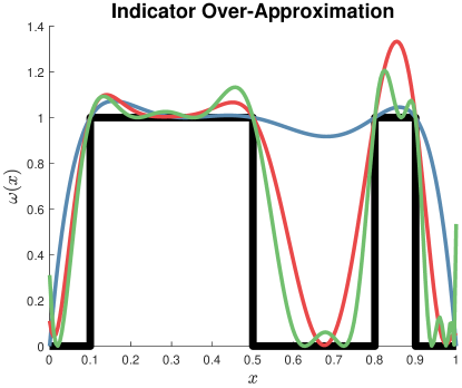
Figure 1: Polynomial over-approximations to $L=[0.1,0.5]\cup[0.8,0.9]$

Table 1: Polynomial approximation order and volume bounds.

Function	$k=6$	$k=20$	$k=120$	Truth
Volume (upper)	0.9269	0.7472	0.6740	0.5

Even though the 1-sublevel sets of Figure 1 are very close to $L$, the volume bounds in Table 1 are far from the true value of 0.5. Unfortunately, there does not exist an efficient method to compute the volume of polynomial sublevel sets purely from the polynomial’s coefficients [52]. This large gap in volume estimates is due to an oscillatory Gibbs phenomenon [53] involved in the approximation of the discontinuous $I_{L}$ by the set of continuous polynomials. The presence of Gibbs phenomena contributes towards an asymptotic convergence rate of $O(1/\log\log k)$ in the error of volume approximation [34].

Stokes methods (introduced further in Section 6) [36] can be used to refine volume estimates and yield faster convergence in $k$ through the addition of redundant derivative constraints.

3 Slice-Volume

This section will solve the slice-volume Problem 1 using infinite-dimensional LPs. We will begin with the following assumption:

• There exists an $R\in[0,\infty)$ such that $L\subseteq B_{R}^{n}$.

The ball constraint $R^{2}-\lVert x\rVert^{2}$ can be added to the description of any BSA $L$ satisfying A1 without changing its geometry.

3.1 Slice-Volume Variables and Supports

The variables used in the slice-volume optimization problem are listed in Table 2.

Table 2: Variables in slice-volume analysis

$\theta$	Direction
$t$	Affine Offset
$Z$	Local Coordinate Frame
$y$	Local Coordinate on the plane $\theta\cdot x=t$

The support sets involving variables in Table 2 are

$$\Omega =\{(\theta,t)\in S^{n}\times[-R,R]\}$$ (7a)

$$\Omega_{Z} =\{(\theta,t,Z)\in S^{n}\times[-R,R]\times\mathbb{R}^{n\times(n-1)}\mid[\theta,Z]\in O(n)\}$$ (7b)

$$\Psi =\Omega_{Z}\times B_{R}^{n-1}$$ (7c)

$$\Psi_{L} =\Psi\cap\{(\theta t+Zy)\in L\}$$ (7d)

The domain of the $R$-truncated Radon transform (2) is $\Omega$ from (7a). The set $\Psi_{L}$ represents $L$ via the over-complete formulation of $x=\theta t+Zy$. Constraints (7b) and (7d) implies that $Z\in\mathbb{V}_{n-1}(\mathbb{R}^{n})$.

Figure 2 visualizes the slicing geometry and variables from Table 2. The set $L$ is the region inside the outer gray ellipsoid and outside the inner red ellipsoid. The green arrow is the slicing direction $\theta$, and the two black arrows are the columns of $Z$. The value $t$ is the affine offset in the direction of $\theta$ between the origin (center of the coordinate frame) and the blue slicing plane. In this manner, a point $x\in L$ (black asterisk) may be represented by an appropriate choice of $x=\theta t+Zy.$

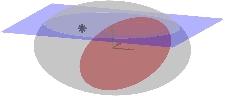
Figure 2: Slicing geometry and variables from Table 2.

3.2 Slice-Volume Function Program

A functional LP for the slice-volume task will be developed based on the smooth-indicator-approximating volume computation methodology from Section 2.3. For notational convenience, let us use define the $y$-integration $\Lambda_{R}:C(\Psi)\rightarrow C(\Omega_{Z})$ as $\forall w(\theta,t,Z,y)\in C(\Psi)$:

$$\Lambda_{R}w(\theta,t,Z)=\int_{B_{R}^{n-1}}w(\theta,t,Z,y)dy.$$ (8)

We introduce a continuous auxiliary function variable $w(\theta,t,Z,y)$ in order to pose the following slice-volume maximization program:

$$p^{*}= \inf_{\gamma\in\mathbb{R}}\quad\gamma$$ (9a)

$$\gamma\geq\Lambda_{R}w(\theta,t,Z) \forall(\theta,t,Z)\in\Omega_{Z}$$ (9b)

$$w(\theta,t,Z,y)\geq 1 \forall(\theta,t,Z,y)\in\Psi_{L}$$ (9c)

$$w(\theta,t,Z,y)\geq 0 \forall(\theta,t,Z,y)\in\Psi$$ (9d)

$$w(\theta,t,Z,y)\in C(\Psi).$$ (9e)

Lemma 3.1.

Program (9) is an upper-bound on Problem 1 ($p^{*}\geq P^{*}$).

Proof.

The indicator function $w^{*}(\theta,t,Z,y)=I_{\Psi}$ will satisfy constraints (9c)-(9d) while ignoring the continuity requirement in (9e). The integrated term $\Lambda_{R}w^{*}(\theta,t,Z)$ may be interpreted as the radon transform $\mathcal{R}I_{L}(\theta,t)$ with respect to an arbitrary coordinate frame $Z\in\mathbb{V}_{n-1}(\mathbb{R}^{n})$. Every value $\gamma$ such that $\forall(\theta,t,Z)\in\Omega_{Z}:\ \gamma\geq\mathcal{R}I_{L}(\theta,t)$ (9b) is an upper-bound on the maximal slice volume.

Letting $w$ be any continuous feasible solution (9c)-(9e), it holds that $w\geq w^{*}$ pointwise and also that $\Lambda_{R}w(\theta,t,Z,y)\geq\mathcal{R}I_{L}(\theta,t)$ at each $(\theta,t)\in\Omega$. It therefore holds that $p^{*}\geq P^{*}$.

∎

In order to prove equality between Problem 1 and the infimum of (9), we require a notion of almost uniform convergence [54, 55]:

Definition 3.1.

A sequence of functions $\{f_{n}\}_{n}$ converges to $f$ almost uniformly in a set $X$ if for every $\epsilon>0$, there exists $A\subset X$ such that $\textrm{Vol}(A)<\epsilon$ and $f_{n}\rightarrow f$ uniformly on $X\setminus A$.

Theorem 3.2.

Under A1, there is no relaxation gap between Problem 1 and Program (9) ($p^{*}=P^{*}$).

Proof.

The set $C(\Psi)$ is dense in $L^{1}(\Psi)$, implying the existence of a sequence of functions $w^{k}(\theta,t,Z,y)\in C(\Psi)$ converging to $w^{*}$ from above in an $L^{1}$ sense:

$$w^{k}\geq w^{*},\qquad\lim_{k\rightarrow\infty}\int_{\Psi}\left(w^{k}(\theta,t,Z,y)-w^{*}(\theta,t,Z,y)\right)d\theta\;dt\;dZ\;dy=0.$$ (10)

By Theorem 2.5.3 of [54], $L_{1}$-convergence of $w^{k}$ implies the existence a subsequence $w^{k^{\prime}}$ converging to $w^{*}$ almost uniformly.

It therefore holds that $\{\Lambda_{R}w_{k}(\theta,t,Z)\}_{k}$ converges almost uniformly to $\mathcal{R}I_{L}(\theta,t)$. The pointwise upper-bound of $w^{k}\geq w^{*}$ ensures that the infimum will therefore be maintained, though a minimum may not be met (in general).

∎

Corollary 1.

The objective value $p^{*}$ from (9) is finite under A1.

Proof.

Bounded from above: The function $w(\theta,t,Z,y)=1$ is feasible for constraints (9c) - (9e). The choice of $\gamma=\Lambda_{R}(1)=\int_{B_{R}^{n-1}}1dy=\textrm{Vol}_{n-1}(B_{R}^{n-1})$ is feasible for (9b), given that $R$ is finite by A1.

Bounded from below: In the case where $L=\varnothing$, the function $w=0$ would be the minimal possible choice satisfying (9c) - (9e).

As such, the optimal value $p^{*}$ is bounded between $[0,\textrm{Vol}_{n-1}(B_{R}^{n-1})].$ ∎

Example 3.1.

This pathological example will demonstrate almost uniform convergence of the slice-volume construction. In this example, we will restrict $t=0$ to aid in explanation. Consider the 1-dimensional disc set $L=\{x\in\mathbb{R}^{2}\mid x_{2}=0\}\cap B_{R}^{2}$ with $R\in(0,\infty)$. The discontinuous Radon transform of the indicator function of $L$ is

$$\mathcal{R}I_{L}(\theta,0)=\begin{cases}2R&\theta=\pm(0,1)\\ 0&\textrm{else}.\end{cases}$$ (11)

Let $\eta\in(0,R\sqrt{2}/2)$ be a tolerance. We can construct a sequence of functions $f_{\eta}(x)\geq I_{L}(x)$ by defining

$$f_{\eta}(x)=\begin{cases}1-\lvert x_{2}\rvert/\eta&\lvert x_{2}\rvert\leq\eta\\ 0&\textrm{else}.\end{cases}$$ (12)

The planar direction $\theta\in S^{1}$ will be parameterized by an angle $\phi\in[0,2\pi]$ under the relation $\theta=[\cos(\phi+\pi/2),\sin(\phi+\pi/2)]$. The Radon transform of $f_{\eta}$ at the translate $t=0$ in the domain $\phi\in[0,\pi/2]$ is

$$\mathcal{R}f_{\eta}(\phi,0)=\begin{cases}\eta/\cos(\pi/2-\phi)&\phi\in[\pi/4,\pi/2]\\ \eta/\sin{\phi}&\phi\in[\sin^{-1}(\eta/R),\pi/4]\\ R(2-(R/\eta)\sin{\phi})&\phi\in[0,\sin^{-1}(\eta/R)].\end{cases}$$ (13)

The transform in (13) can be extended to $[0,2\pi]$ by symmetry. Under this definition for $f_{\eta}$,

$$\mathcal{R}f_{\eta}(\phi,0) =2R, \mathcal{R}f_{\eta}(\sin^{-1}(\eta/R),0) =R, \mathcal{R}f_{\eta}(\pi/2,0) =\eta.$$ (14)

For any $\epsilon^{\prime}>0$, we can compute the angle of $\phi^{\prime}=\sin^{-1}(\eta/\epsilon^{\prime})$. The volume of $\phi\in[0,2\pi]$ with $\mathcal{R}f_{\eta}(\phi,0)>\epsilon^{\prime}$ is $4\phi^{\prime}$. Given an $\epsilon>0$ with $\epsilon^{\prime}=\epsilon/4$, we can choose a $\eta$ and a $\phi^{\prime}$ such that $4\phi^{\prime}\leq\epsilon$. This provides almost uniform convergence, because $\eta$ and $f_{\eta}$ can be chosen to ensure that the volume $4\phi^{\prime}\rightarrow 0$ as $\epsilon\rightarrow 0$.

3.3 Slice-Volume Measure Program

A dual program to (9) can be derived by introducing measure variables,

Table 3: Variables in slice-volume measure LP

$\mu_{0}\in\mathcal{M}_{+}(\Omega_{Z})$	Choice of slicing direction $(t,\theta)$ and coordinate frame $Z$
$\mu\in\mathcal{M}_{+}(\Psi_{L})$	Volume tracking
$\hat{\mu}\in\mathcal{M}_{+}(\Psi)$	Slack measure

Define $\lambda_{R}^{n-1}$ as the Lebesgue measure of the ball $B^{n}_{R}$. A convex measure LP that relaxes Problem 1 is:

$$m^{*}= \sup\ \langle 1,\mu\rangle$$ (15a)

$$\mu_{0}\otimes\lambda_{R}^{n-1}=\mu+\hat{\mu}$$ (15b)

$$\langle 1,\mu_{0}\rangle=1$$ (15c)

$$\mu_{0}\in\mathcal{M}_{+}(\Omega_{Z}),$$ (15d)

$$\hat{\mu}\in\mathcal{M}_{+}(\Psi)$$ (15e)

$$\mu\in\mathcal{M}_{+}(\Psi_{L}).$$ (15f)

The measure $\mu_{0}$ is a probability distribution over $(\theta,t,Z)$ that picks out the best direction $\theta$, offset $t$, and coordinate frame $Z$ for a slice. The objective in (15a) is the supremal slice-volume.

Theorem 3.3.

Program (15) is an upper-bound on Problem 1 with $m^{*}\geq P^{*}$.

Proof.

Let $(\theta^{\prime},t^{\prime})\in\Omega$ be a slicing direction and offset. We will now construct measures from Table 3 from $(\theta,t)$ that are feasible for (15b)-(15f). Let $Z^{\prime}\in\mathbb{R}^{(n-1)\times n}$ be a matrix such that $[\theta^{\prime},\,Z^{\prime}]\in O(n)$. We let $\mu_{0}^{\prime}=\delta_{\theta=\theta^{\prime}}\otimes\delta_{t=t^{\prime}}\otimes\delta_{Z=Z^{\prime}}$ be a probability distribution representing the slicing choice $(\theta^{\prime},t^{\prime},Z^{\prime})$.

We can construct a set $Y=\{y\in B^{n-1}_{R}\mid\theta^{\prime}t^{\prime}+Z^{\prime}y\in L\}$ that has a Lebesgue measure $\lambda_{Y}\leq\lambda_{R}^{n-1}$. The measures of $\mu^{\prime}=\mu_{0}^{\prime}\otimes\lambda_{Y}$ and $\hat{\mu}^{\prime}=\mu_{0}^{\prime}\otimes\otimes\lambda_{\textrm{cl}(B^{n-1}_{R}-Y)}$ can therefore be defined to satisfy the domination relation (15b).

A measure solution $(\mu_{0}^{\prime},\hat{\mu}^{\prime},\mu^{\prime})$ therefore exists for every possible choice of $(\theta^{\prime},t^{\prime})\in\Omega$. The feasible set of measures is therefore a superset of the (induced) feasible set of $\Omega,\Omega$, implying that $m^{*}\geq P^{*}$. ∎

Lemma 3.4.

The measure solutions to (15) are bounded under A1.

Proof.

Boundedness of nonnegative measures will be proven using the sufficient combination of compact support and finite mass. Assumption A1 ensures that $L$ is compact with finite $R$. The set $\Omega_{Z}=S^{n-1}\times[-R,R]\times\mathbb{V}_{n-1}(\mathbb{R}^{n})$ is compact, as is the set $\Psi$. The set $\Psi_{L}$ is contained within the compact set $\Psi$, since $\Psi_{L}$ is the preimage of the compact set $L$ under the continuous mapping $\theta t+Zy$.

The mass of $\mu_{0}$ is set to 1 by (15c).

$$\langle 1,\mu\rangle+\langle 1,\hat{\mu}\rangle=\langle 1,\mu_{0}\otimes\lambda_{R}^{n-1}\rangle=(1)(\textrm{Vol}_{n-1}{B_{R}^{n-1}})=\textrm{Vol}_{n-1}{B_{R}^{n-1}}<\infty.$$ (16)

Because $\mu$ and $\hat{\mu}$ are each nonnegative measures, their masses are likewise nonnegative numbers. Their masses therefore satisfy $\langle 1,\mu\rangle,\langle 1,\hat{\mu}\rangle\in[0,\textrm{Vol}_{n-1}{B_{R}^{n-1}}].$

∎

Theorem 3.5.

Strong duality holds between programs (9) and (15) under A1.

Proof.

See Appendix A. ∎

4 Slice-Volume Semidefinite Programs

This section will apply the moment-SOS hierarchy of SDP towards solution to (9).

4.1 Slice-Volume SOS Program

We will restrict $w$ from (9e) to be a polynomial $w\in\mathbb{R}[\theta,t,Z,y]_{\leq 2k}$ for some degree $k\in\mathbb{N}$. The following proposition is required in order to evaluate the integral from (9b):

Proposition 4.1 (Theorem 3.1 of [56]).

The moments of the Lebesgue distribution for the radius-$R$ ball in $n$ dimensions are

$$\forall\alpha\in\mathbb{N}^{n}:\qquad\int_{B^{n}}y^{\alpha}dy=R^{n+\lvert\alpha\rvert}\frac{\prod_{i}\Gamma((\alpha_{i}+1)/2)}{\Gamma(1+(n+\lvert\alpha\rvert)/2)}.$$ (17)

We will now be assuming that $L$ has BSA BSA structure:

• The set $L$ is BSA BSA set that includes a ball constraint description $R^{2}-\lVert x\rVert_{2}^{2}\geq 0$.

Problem 2.

The degree-$k$ SOS truncation of (9) is:

$$p^{*}_{k}= \inf_{\gamma\in\mathbb{R}}\quad\gamma$$ (18a)

$$\gamma-\textstyle\Lambda_{R}w(\theta,t,Z)\in\Sigma[\Omega_{Z}]_{\leq 2k}$$ (18b)

$$w(\theta,t,Z,y)-1\in\Sigma[\Psi_{L}]_{\leq 2k}$$ (18c)

$$w(\theta,t,Z,y)\in\Sigma[\Psi]_{\leq 2k}$$ (18d)

$$w(\theta,t,Z,y)\in\mathbb{R}[\theta,t,Z,y]_{\leq 2k}.$$ (18e)

Theorem 4.2.

Program (18) provides a decreasing sequence of upper bounds $p_{k}^{*}\geq p^{*}_{k+1}\geq\ldots$ that converges as $\lim_{k\rightarrow\infty}p_{k}^{*}=P^{*}$ under assumptions A1 and A2.

Proof.

See Appendix B. ∎

Remark 1.

The WSOS Constraint (18b) has a polynomial $\sigma_{0}(\theta,t,Z)\in\Sigma[\theta,t,Z]_{\leq 2k}$ in representation (6). The Gram matrix of $\sigma_{0}$ is a PSD variable in the SDP formulation of problem (18). The dual PSD variable to this Gram matrix is associated with the moment matrix of $\mu_{0}$ [30]. If the output of SDP SDP solver for (18) yields a low-rank dual variable (candidate moment matrix for $\mu_{0}$), then the matrix-factorization-based methods of [57] can be used to attempt extraction of (an orbit of) candidates $(\theta,t,Z)$ to solve (15).

4.2 Extension to Semialgebraic Sets

Assume that $L$ may be expressed as the union of $N_{c}$ BSA sets $L=\cup_{j=1}^{N_{c}}L_{j}$, in which each $L_{j}$ possesses $(R^{2}-\lVert x\rVert_{2}^{2}\geq 0)$ in its BSA representation. Constraint (18b) can be generalized to $\forall j\in 1..N_{c}:\ w(\theta,t,y)-1\in\Sigma[\Psi_{L_{j}}]_{\leq 2k}$ in the union case, while retaining convergence as $\lim_{k\rightarrow\infty}p_{k}^{*}=P^{*}.$

In this manner, lower-bounds for the minimum slice-volume of $L$ can be found by maximizing the slice-volume over the complement of $L$ (which can be represented as a union of BSA sets).

Slice-volumes can also be computed for semialgebraic sets described by given projections. Let $L\subset X$ and $\hat{L}\subset X\times E$ be sets such that $L=\pi^{x}\hat{L}$ and $\hat{L}$ is BSA. This implies that $L$ is semialgebraic (projection of BSA BSA set). Constraint (18c) can then be implemented as WSOS WSOS constraint over the following BSA set:

$$\Psi_{\hat{L}} =\{(\theta,t,Z,y,e)\in\Psi\times E\mid\exists e:(\theta t+Zy)\in\hat{L},\ [\theta,\,Z]\in O(n)\}.$$ (19)

4.3 Computational Complexity

This subsection will quantify the computational complexity of solving SDP formulations of (18) via interior point methods. The per-iteration scaling complexity of solving SDP SDP arising from the moment-SOS hierarchy in $N$ variables at degree $k$ (with a single PSD block) is $O(N^{6k})$ and $O(k^{4N})$ [30, 58].

The computational complexity of degree-$d$ SOS tightenings of programs (9) is dominated by the PSD matrix constraints present in (18c) and (18d). These constraints involve the $(n)+(1)+(n-1)+n(n-1)=n^{2}+n$ variables $(\theta,t,Z,y)$. The maximal-size PSD (Gram) matrices will have size $\binom{n^{2}+n+k}{k}$, which quickly grows intractable as $n$ increases. In comparison, constraints (18b) have maximal PSD sizes of $\binom{n+1+k}{k}$ and $\binom{2n+k}{k}$, respectively.

5 Reduction of Computational Complexity

These subsequent sections will detail how algebraic and symmetric structures inside the support sets (7) can be used to reduce the size of the Gram matrices in Section 4.3.

5.1 Dimension-Independent

The slice volume programs offer several forms of extant structure.

5.1.1 Discrete Symmetry

To begin with, the Radon transform of a function is symmetric under the exchange $(\theta,t)\leftrightarrow(-\theta,-t)$ (in domain $\Omega$). As a result, the functions $(w,\tilde{w})$ may be chosen to be even under the exchange $(\theta,t,Z,y)\leftrightarrow(-\theta,-t,-Z,-y)$ (in domain $\Psi$). This is an instance of a sign-symmetry, which can be exploited through the SOS methods developed in [59, 60]. Symmetries perform a block-diagonalization of the Gram matrices, yielding a sequence of smaller PSD constraints while retaining the same degree-$k$ optimal value.

5.1.2 Continuous Symmetry

The set $\Psi_{L}$ admits an $O(n-1)$ symmetry. For any $Q\in O(n-1)$ and $(\theta,t,Z,y)\in\Psi_{L}$, it holds that $(\theta,t,ZQ^{T},Qy)\in\Psi_{L}$ (because $\theta t+Zy=\theta t+(ZQ^{T})(Qy)$). The function $w(\theta,t,Z,y)$ can be chosen to respect this orthogonal symmetry without changing the objective value of (9), because the Radon transform function $\mathscr{R}I_{L}(\theta,t)$ used in the proof of lemma 3.1 is $Z$-independent.

Further symmetries can be exploited if $L$ also possesses geometric symmetries (e.g., dihedral).

5.1.3 Quotient Reduction

The impositions of $\lVert\theta\rVert_{2}^{2}=1$ and $[\theta,Z]$ in the descriptions of $\Omega$ and $\Psi_{L}$ yield a sequence of degree-2 polynomial equality constraints. Gröbner basis reduction methods [61] can be used to further reduce the size of the Gram matrices [62, 63]. As an example, the replacement rule of $\theta_{n}^{2}\mapsto 1-\sum_{i=1}^{n-1}\theta_{i}^{2}$ would be evaluated anywhere $\theta_{n}^{2}$ appears in a WSOS polynomial expression. It is therefore not necessary for the polynomial $v$ or any WSOS multiplier to contain a monomial with a degree-$\geq 2$ term in $\theta_{n}$.

5.2 Dimension 2, 4, 8

A manifold $\mathcal{M}$ is parallelizable if there exists a continuous map between $\mathcal{M}$ and the space of coordinate frames on $\mathcal{M}$ (the tangent bundle of $\mathcal{M}$ is trivial).

The sphere $S^{n^{\prime}}$ is parallelizable only in dimensions $n^{\prime}=\{1,3,7\}$ by Corollary 2 of [64]. These choices correspond to the division rings defined at $n=n^{\prime}+1=\{2,4,8\}$ of complex numbers, quaternions, and octonions. The basis for the tangent space may be constructed by forming multiplication tables of these division rings [64].

In dimension $n=2$ with $\theta\in S^{1}$ corresponding to complex numbers $\theta_{1}+i\theta_{2}$, the frame $Z$ satisfies

$$[\theta,Z] =\begin{bmatrix}\theta_{1}&-\theta_{2}\\ \theta_{2}&\theta_{1}\end{bmatrix}.$$ (20a)

The process can be repeated for quaternions $$\theta=\theta_{1}+\theta_{2}i+\theta_{3}j+\theta_{4}k\in S^{3}$$ as

$$[\theta,Z] =\begin{bmatrix}\theta_{1}&-\theta_{2}&-\theta_{3}&\theta_{4}\\ \theta_{2}&\theta_{1}&-\theta_{4}&-\theta_{3}\\ \theta_{3}&-\theta_{4}&\theta_{1}&-\theta_{2}\\ \theta_{4}&\theta_{3}&\theta_{2}&\theta_{1}\end{bmatrix},$$ (20b)

and similarly for octonions with

$$[\theta,Z] =\begin{bmatrix}\theta_{1}&-\theta_{2}&-\theta_{3}&\theta_{4}&-\theta_{5}&\theta_{6}&\theta_{7}&-\theta_{8}\\ \theta_{2}&\theta_{1}&-\theta_{4}&-\theta_{3}&-\theta_{6}&-\theta_{5}&\theta_{8}&\theta_{7}\\ \theta_{3}&-\theta_{4}&\theta_{1}&-\theta_{2}&-\theta_{7}&\theta_{8}&-\theta_{5}&\theta_{6}\\ \theta_{4}&\theta_{3}&\theta_{2}&\theta_{1}&-\theta_{8}&-\theta_{7}&-\theta_{6}&-\theta_{5}\\ \theta_{5}&-\theta_{6}&-\theta_{7}&\theta_{8}&\theta_{1}&-\theta_{2}&-\theta_{3}&\theta_{4}\\ \theta_{6}&\theta_{5}&-\theta_{8}&-\theta_{7}&\theta_{2}&\theta_{1}&-\theta_{4}&-\theta_{3}\\ \theta_{7}&-\theta_{8}&\theta_{5}&-\theta_{6}&\theta_{3}&-\theta_{4}&\theta_{1}&-\theta_{2}\\ \theta_{8}&\theta_{7}&\theta_{6}&\theta_{5}&\theta_{4}&\theta_{3}&\theta_{2}&\theta_{1}\end{bmatrix}.$$ (20c)

Substitutions in (20) form a (nonunique) explicit representation of $Z$ in terms of $\theta$. As a result, constraints such as in (9c) will only contain the $2n$ variables $(\theta,t,y)$ (down from $n^{2}+n$). The maximal-size PSD matrix of (18c) is reduced from $\binom{n^{2}+n+k}{k}$ to $\binom{2n+k}{k}$ by virtue of eliminating $Z$ when $n\in\{2,4,8\}$.

The specific selection of a $Z$ matrix in terms of $\theta$ will destroy the continuous $O(n-1)$ symmetry from Section 5.1.2. Breaking the $O(n-1)$ symmetry is acceptable, due to the elimination of $Z$ in the count of the number of variables.

5.3 Dimension 3

The sphere $S^{2}$ (embedded in 3-dimensional Euclidean space) is not parallelizable [64], and therefore $Z$ cannot be assigned to $\theta$ in a continuous manner. Such a topological obstruction prevents the definition of a polynomial-valued map $\theta\rightarrow Z$ from (20) because polynomial structure is stronger than continuity.

Given that a polynomial (continuous) parameterization of $Z$ in terms of $\theta$ alone does not exist in $n=3$, we instead parameterize $Z$ in terms of $\theta\in S^{2}$ and a new variable $b\in S^{2}$ using the existence of the three-dimensional cross-product $\times$ operator. For any $b\in S^{2}$ with $\theta\cdot b=0$, a three-dimensional orthogonal coordinate frame can be created as

$$\begin{bmatrix}\theta&Z\end{bmatrix}=\begin{bmatrix}\theta&b&\theta\times b\end{bmatrix}.$$ (21)

The frame (21) can be used to construct the following set:

$$\Psi_{L}^{3} =\{(\theta,t,b,y)\in\Omega\times S^{2}\times B_{R}^{2}\mid(\theta t+by_{1}+(\theta\times b)y_{2})\in L,\ \theta\cdot b=0\}.$$ (22)

The set $\Psi_{L}^{3}$ from (22) has 9 variables $(\theta,t,y,b)$, which is fewer than the $3^{2}+3=12$ variables needed to represent $\Psi_{L}$ from (7d) in terms of $(\theta,t,Z,y)$. The symmetric and algebraic structures from Section 5.1 are retained in the 3-dimensional case. We note that a possible Gröbner basis of $\{\lVert\theta\rVert_{2}^{2}=1,\lVert b\rVert_{2}^{2}=1,\theta\cdot b=0\}$ in the graded lexicographical ordering is:

$$\lVert\theta\rVert_{2}^{2}-1, \theta_{1}(b_{2}^{2}+b_{3}^{2}-1)-b_{1}(\theta_{2}b_{2}-\theta_{3}b_{1}),$$

$$\lVert b\rVert_{2}^{2}-1, \theta_{1}(\theta_{2}b_{2}+\theta_{3}b_{3})+b_{1}(-\theta_{2}^{2}-\theta_{3}^{2}+1),$$ (23)

$$\theta\cdot b, \theta_{1}(\theta_{2}b_{3}^{2}-\theta_{3}b_{2}b_{3}-\theta_{2})+b_{1}(b_{2}-\theta_{2}\theta_{3}b_{3}+\theta_{3}b_{2}),$$

$$\theta_{2}(\theta_{2}b_{3}^{2}-2\theta_{3}b_{2}b_{3}-\theta_{2})+\theta_{3}^{2}(b_{2}^{2}-1)-b_{2}^{2}-b_{3}^{2}+1.$$

The set description $\Psi_{L}^{3}$ possesses an $SO(2)$ symmetry, which is a subgroup of the full $O(2)$ symmetry from Section 5.1.2.

Lemma 5.1.

The three-dimensional set $\Psi_{L}^{3}$ is $SO(2)\times\mathbb{Z}_{2}$-invariant.

Proof.

The $\mathbb{Z}_{2}$ symmetry is described in Section (5.1.1) with respect to the mapping $(\theta,t,y,b)\leftrightarrow(-\theta,-t,-y,-b)$. We now focus on the $SO(2)$ symmetry. Let $Q$ be an orthogonal matrix to transform in the local $y$-plane as

$$Q=\begin{bmatrix}Q_{1}&Q_{2}\\ Q_{3}&Q_{4}\end{bmatrix}\in O(2),$$ (24)

and let $(\theta,t,b,y)$ be an arbitrary point in $\Psi_{L}^{3}$. Define the quantities $(Z^{\prime},b^{\prime},y^{\prime})$ as

$$Z^{\prime} =\begin{bmatrix}b&\theta\times b\end{bmatrix}Q^{T} b^{\prime} =Z^{\prime}\begin{bmatrix}1\\ 0\end{bmatrix} \theta\times b^{\prime} =Z^{\prime}\begin{bmatrix}0\\ 1\end{bmatrix} y^{\prime} =Qy.$$ (25)

It holds that

$$\lVert b^{\prime}\rVert_{2}^{2} =\lVert(Q_{1}b+Q_{3}(\theta\times b))\rVert_{2}^{2}=Q_{1}^{2}\lVert b\rVert_{2}^{2}+Q_{3}^{2}\lVert\theta\times b\rVert_{2}^{2}=1$$ (26a)

$$\theta\cdot b^{\prime} =Q_{1}(\theta\cdot b)+Q_{3}\theta\cdot(\theta\times b)=0$$ (26b)

$$(\theta\times b^{\prime})\cdot(Z^{\prime}[0;1]) =Q_{1}Q_{2}b\cdot(\theta\times b)+Q_{1}Q_{4}\lVert\theta\times b\rVert_{2}^{2}-Q_{2}Q_{3}\lVert b\rVert_{2}^{2}-Q_{3}Q_{4}b\cdot(\theta\times b)$$ (26c)

$$=Q_{1}Q_{4}-Q_{3}Q_{2}=\textrm{det}(Q),$$ (26d)

which implies that $(\theta\times b^{\prime})=Z^{\prime}[0;1]$ when $\textrm{det}(Q)=1$. The implication $(\theta,t,b,y)\in\Psi^{3}_{L}\implies(\theta,t,b^{\prime},y^{\prime})\in\Psi^{3}_{L}$ will be valid when $\textrm{det}(Q)=1$, which is valid only in the subgroup $SO(2)\subset O(2)$.

∎

The $SO(2)$ restriction arises from the imposition of the unique cross-product vector $\theta\times b$ when forming $Z$. Just like in Section 5.2, the loss of symmetry (from $O(2)$ to $SO(2)$) is outweighed by the decrease in computational complexity (12 variables down to 9 variables).

6 Stokes Constraints

SOS-truncations to the slice-volume program (in (18)) are vulnerable to slow convergence due to the presence of Gibbs phenomena when $w$ is upper-bounding an indicator function in (18c). This section will utlize the Stokes constraint method of [36] in order to improve the numerical convergence of SOS approximations while keeping the LP objective the same.

6.1 Stokes Constraints Background

We will begin by briefly reviewing Stokes’ Theorem and the Stokes constraint formulation for volume approximation from [35, 36]. Section 6.1.3 presents new work in incorporating symmetries into Stokes constraints. Refer to sections 2 and 3 of [37] for further information about Stokes constraints for BSA sets.

6.1.1 Stokes’ Theorems

The classical Stokes’ theorem is defined with respect to a smooth manifold. We will restrict our presentation to a bounded setting.

Theorem 6.1.

Let $M\subset\mathbb{R}^{n}$ be a compact smooth manifold ($\partial M$ is $C^{1}$). Then for all continuous $(n-1)$-forms $\omega$, it holds that

$$\int_{\partial M}\omega=\int_{M}d\omega.$$ (27)

Stokes’ theorem in (6.1) is applicable in the BSA setting in which $M$ is defined as $M=\{x\mid g_{0}(x)\geq 0\}$ for a $g_{0}\in\mathbb{R}[x]$ such $\partial M=\{x\mid g_{0}(x)=0\}$, and that the $g_{0}(x)=0$ level set is singularity-free.

Stokes’ theorem may be generalized to sets with nonsmooth structure, such as with corners and singular boundaries. One extension to Stokes’ theorem uses the concept of Standard Domains [65]:

Definition 6.1.

Let $S\subset\mathbb{R}^{n}$ be a bounded, open, connected set. Let $\Delta=\textrm{cl}(S)-S$ be the boundary of $S$. $S$ is a standard domain if it obeys the following properties:

1. There exists a set $Q\subset\Delta$ in which $Q$ has zero measure w.r.t. the Hausdorff measure of $\sigma_{\textrm{cl}(S)}$.

2. For each point $p\in\Delta-Q$, there exists a coordinate assignment $p\mapsto[\theta(p);Z(p)]\in O(n)$, local coordinates $\alpha$ with $x=[\theta(p),\;Z(p)]\alpha$, a neighborhood $N_{p}\ni p$, and a smooth function $h\in C^{1}(N_{p})$.

3. Points in $\Delta\cap N_{p}$ can be represented as $\alpha_{1}=h(\alpha_{2},\ldots,\alpha_{n})$.

4. Points in $S\cap N_{p}$ can be represented as $\alpha_{1}>h(\alpha_{2},\ldots,\alpha_{n})$.

Remark 2.

The interiors of full-dimensional polytopes are examples of standard domains.

Theorem 6.2 (Theorem 14.A of [65]).

Let $S$ be a standard domain, and let $Q$ and $\Delta$ be chosen in accordance with Definition 6.1. Further assume that $\omega$ is summable over $\Delta,$ $d\omega$ is summable over $S$, $\omega$ is continuous and bounded in $\text{cl}(S)-Q$, and $\omega$ is smooth in $S$. Then

$$\int_{\text{cl}(S)-S}\omega=\int_{S}d\omega.$$ (28)

Refer to [66] for other formulations of Stokes’ theorems towards nonsmooth boundaries (including for fractals).

6.1.2 Stokes Constraints for Volume Approximation

This subsection will summarize the presentation for Lemma 4.1 of [36] and Equation 4.16 of [67] with a focus on BSA sets described by multiple polynomial inequality constraints.

Consider the $n$-dimensional volume approximation problem from of (4) and (5) with respect to BSA BSA set $L=\{x\mid\forall i:g_{i}(x)\geq 0\}$. Let $\lambda_{L}$ and $\sigma_{L}$ be the Lebesgue and Hausdorff measures of $L$, such that $(\lambda_{L},\lambda_{X}-\lambda_{L})$ is the optimal solution of (5). Define $L_{i}=\{x\mid g_{i}(x)=0,\ g_{-i}(x)\geq 0\}$ as the $i$-th ‘face’ of $\partial L$. For every function $\zeta\in C^{1}(\partial L),$ it holds from the definition of $\partial L$ that

$$\sum_{i=1}^{L}\left(\int_{L_{i}}g_{i}(x)\zeta(x)d\sigma_{L}\right)=0,$$ (29)

because the face $L_{i}$ is defined by $g_{i}(x)=0$.

We will require new assumptions throughout this work:

• The set $\textrm{int}(L)$ is a standard domain.

• The set $L$ satisfies for each $i$ that $\forall x\in L:\nabla g_{i}(x)\neq 0$.

A consequence of A4 is that the normal-vector map pointing out of $L_{i}$ is well-defined with

$$\vec{\mathbf{n}}_{i}(x)=\nabla g_{i}(x)/\lVert\nabla g_{i}(x)\rVert.$$ (30)

Remark 3.

The standard domain description of $L$ is valid with respect to $\textrm{int}(L_{i})=\{x\mid g_{i}(x)=0,\ g_{-i}(x)>0\}$. Given that $g_{i}(x)=0$ on the boundary component $L_{i}$, it holds that $\forall\zeta_{L}\in C^{1}(\partial L):\int_{L_{i}}g_{i}(x)\zeta(x)d\sigma_{L}(x)=\int_{\textrm{int}(L_{i})}g_{i}(x)\zeta(x)d\sigma_{L}(x)$.

For any function $u\in C^{1}(L)^{n}$, the following relation may be computed:

$$\int_{L}\nabla_{x}\cdot u(x)dx =\sum_{i=1}^{L}\int_{\textrm{int}L_{i}}{u(x)\cdot\vec{n}_{i}(x)d\sigma_{L}(x)}$$ (31a)

$$=\sum_{i=1}^{L}\int_{\textrm{int}L_{i}}{(u(x)\cdot\nabla g_{i}(x))/\lVert\nabla_{x}g_{i}(x)\rVert d\sigma_{L}(x)}.$$ (31b)

Defining $$\nu_{i}\in\mathcal{M}_{+}(L_{i}) 1/\lVert\nabla_{x}g_{i}(x)\rVert \sigma_{L} L_{i}$$ as a measure with density with respect to on , the above sum can be expressed as

$$\int_{L}\nabla_{x}\cdot u(x)dx =\sum_{i=1}^{L}\int_{\textrm{int}L_{i}}{(u(x)\cdot\nabla_{x}g_{i}(x))d\nu_{i}}.$$ (31c)

The unique optimum $(\mu,\hat{\mu})=(\lambda_{L},\lambda_{X}-\lambda_{L})$ to (5) must therefore furnish the existence of measures $\tilde{\nu}_{i}\in\mathcal{M}_{+}(\textrm{int}({L_{i}}))$ such that $\forall u\in C(L)^{1}$:

$$\langle\nabla_{x}\cdot u(x),\mu(x)\rangle =\textstyle\sum_{i=1}^{L}\langle u(x)\cdot\nabla_{x}g_{i}(x),\tilde{\nu}_{i}(x)\rangle.$$ (32)

We can extend $\tilde{\nu}_{i}\in\mathcal{M}_{+}(\textrm{int}({L_{i}}))$ to $\nu_{i}\in\mathcal{M}_{+}({L_{i}})$ given that $\partial L_{i}$ has measure 0 with respect to $\sigma_{L_{i}}$, and given that A4 ensures that the density $1/\lVert\nabla g_{i}\rVert$ is bounded over $L_{i}$.

Equation 4.16 of [67] is the augmentation of (5) with the Stokes constraints of

$$\langle\nabla_{x}\cdot u(x),\mu(x)\rangle =\textstyle\sum_{i=1}^{L}\langle u(x)\cdot\nabla_{x}g_{i}(x),\nu_{i}(x)\rangle$$ (33a)

$$\nu_{i}\in\mathcal{M}_{+}(L_{i}).$$ (33b)

Theorem 4.2 of [36] proves that this Stokes infimal volume approximation program achieves its minimum in the case where $L$ is described by the smooth superlevel set of a single polynomial inequality constraint.

6.1.3 Stokes Constraints with Symmetry

Stokes constraints can be introduced to volume approximation methods while respecting a symmetry structure of $L$. This development is motivated by the presence of the discrete and continuous symmetries in the slice-volume program (18) from Section 5.1. For simplicity, we will focus on the discrete sign symmetry from Section (5.1.1) (such as in the $n\in\{2,4,8\}$ case), but will later remark on how the continuous symmetry from Section 5.1.2 can be accomodated.

Let $G$ be a discrete group with finite cardinality $\lvert G\rvert$. The action of $\rho\in G$ on $x\in\mathbb{R}^{n}$ is $x\mapsto\rho x$, and the pullback of a $\rho$-action on a measure $\mu\in\mathcal{M}_{+}(X)$ is $\forall A\in X:\mu(\rho A)$. The measure $\mu$ is invariant under $G$ if $\forall A\in X:\mu(\rho A)=\mu(A)$, and the set of $G$-invariant measures supported on $X$ is $\mathcal{M}_{+}(X)^{G}$. Refer to [68] for more detail about invariant measures and their application in polynomial optimization.

The group-average of a function $f$ over a group $G$ is

$$[f(x)]_{G}=(1/\lvert G\rvert)\sum_{\rho\in G}f(\rho x).$$ (34)

The returned average $f_{G}(x)$ is a $G$-invariant function. The averaging procedure $[\cdot]_{G}$ is also called the Reynolds operator.

The pairing $\langle\cdot,\cdot\rangle$ satisfies

$$\forall f\in C(X),\ \mu\in\mathcal{M}_{+}(X)^{G}: \qquad\langle f,\mu\rangle=\langle f_{G},\mu\rangle.$$ (35)

If the set $L$ is $G$-symmetric, then the Lebesgue measure $\lambda_{X}$ and Hausdorff measure $\sigma_{X}$ are both $G$-invariant. The Stokes constraint in (33) can be equivalently expressed in a $G$-invariant manner as

$$\langle[\nabla_{x}\cdot u(x)]_{G},\mu(x)\rangle =\textstyle\sum_{i=1}^{L}\langle[u(x)\cdot\nabla_{x}g_{i}(x)]_{G},\nu_{i}(x)\rangle.$$ (36)

Remark 4.

In the case where $G$ is an infinite group (with a continuous action) with unique Haar (symmetry-invariant) measure $\nu$, the group average in (34) is taken as the integral $1/\textrm{vol}(G)\int_{\rho\in G}f(\rho x)d\nu(\rho)$.

6.2 Stokes Constraints for Slice-Volume

We adjoin the slice-volume programs (9) and (15) with Stokes-type constraints for volume approximation.

6.2.1 Stokes Measure Program

The Stokes constraint in (33) will be performed with respect to the volume-slice-coordinate $y$.

Define the support set $\Psi_{L}^{i}$ on the boundary of $\Psi_{L}$ as

$$\Psi_{L}^{i} =\Psi_{L}\mid_{g_{i}(\theta t+yZ)=0} \forall i\in 1..N_{c}.$$ (37)

New boundary measures will be defined as in $\nu_{i}\in\mathcal{M}_{+}(\Psi_{L}^{i})$ to form the Stokes scheme.

The slice-volume program has a subgroup $G$ generated by the reflection $G:(\theta,t,Z,y)\leftrightarrow-(\theta,t,Z,y)$. The averaging operation for a function $f(\theta,t,Z,y)$ over this subgroup is

$$[f(\theta,t,Z,y)]_{G} =(f(\theta,t,Z,y)+f(-\theta,-t,-y,-Z))/2.$$ (38)

The induced Stokes constraint from (39a) for the constraint $\forall i:g_{i}(\theta t+Zy)=0$ with respect to the test functions $u\in C^{1}(\Psi_{L})^{n}$ is

$$\langle[\nabla_{y}\cdot u(\theta,t,Z,y)]_{G},\mu(\theta,t,Z,y)\rangle =\textstyle\sum_{i=1}^{L}\langle[u(\theta,t,Z,y)\cdot\nabla_{y}g_{i}(\theta t+Zy)]_{G},\nu_{i}(\theta,t,Z,y)\rangle,$$ (39a)

which will be written in shorthand as

$$[\text{grad}_{y}]_{G}\mu =\textstyle\sum_{i=1}^{L}[\text{grad}_{y}((\theta t+Zy)_{\#}g_{i})]_{G}\nu_{i}.$$ (39b)

Proposition 6.3.

The gradient $\nabla_{y}g_{i}(\theta t+Zy)$ can be computed by the chain rule:

$$\nabla_{y}g_{i}(\theta t+Zy)=Z^{T}\nabla_{x}g_{i}(\theta t+Zy).$$ (40)

This gradient is zero whenever $\theta$ and $\nabla_{y}g_{i}$ are colinear, given that $Z^{T}\theta=0$ from (7d).

Program (15) with Stokes constraints from (39a) has the form of

$$m^{*}_{s}= \sup\ \langle 1,\mu\rangle$$ (41a)

$$\mu_{0}\otimes\lambda_{R}^{n-1}=\mu+\hat{\mu}$$ (41b)

$$\langle 1,\mu_{0}\rangle=1$$ (41c)

$$[\text{grad}_{y}]_{G}\mu=\textstyle\sum_{i=1}^{L}[\text{grad}_{y}(\theta t+Zy)_{\#}g_{i}]_{G}\nu_{i}$$ (41d)

$$\mu_{0}\in\mathcal{M}_{+}(\Omega_{Z}),$$ (41e)

$$\hat{\mu}\in\mathcal{M}_{+}(\Psi)$$ (41f)

$$\mu\in\mathcal{M}_{+}(\Psi_{L})$$ (41g)

$$\nu\in\mathcal{M}_{+}(L_{i}),\ \forall i\in 1..N_{c}.$$ (41h)

Theorem 6.4.

Programs (15) and (41) have the same optimal value with $m^{*}_{s}=m^{*}$ under assumptions A1-A4.

Proof.

Letting $\theta,t\in\Omega$ be an arbitrary slicing direction and offset, we can choose a $Z^{\prime}$ such that $[\theta,Z^{\prime}]\in O(n)$. Defining the set $Y=\{y\in B^{n-1}_{R}\mid\theta^{\prime}t^{\prime}+Z^{\prime}y\in L\}$ with Lebesgue measure $\lambda_{Y}$, the proof of Theorem (3.3) offers feasible variates of $\mu_{0}^{\prime}=\delta_{\theta=\theta^{\prime}}\otimes\delta_{t=t^{\prime}}\otimes\delta_{Z=Z^{\prime}}$, $\mu^{\prime}=\mu_{0}^{\prime}\otimes\lambda_{Y}$, and $\hat{\mu}^{\prime}=\mu_{0}^{\prime}\otimes\lambda_{B^{n-1}_{R}-Y}$.

For each $i\in N_{c}$, define $Y_{i}=\{y\in B^{n-1}_{R}\mid\theta^{\prime}t^{\prime}+Z^{\prime}y\in L_{i}\}$ and let $\sigma_{i}(y)$ be the Hausdorff measure of $y$ over $Y_{i}$. While A4 implies that $\forall x\in L_{i}:\ \nabla_{x}g_{i}(x)\neq 0$, Proposition 6.3 allows for the possibility of points $y\in Y_{i}$ with $\nabla_{y}g_{i}(\theta^{\prime}t^{\prime}+Z^{\prime}y)=0$. It is therefore not possible to select $\xi_{i}^{\prime}$ as unique measure with a density of $1/\lVert\nabla_{y}g(\theta^{\prime}t^{\prime}+Z^{\prime}y)\rVert$ over $\sigma_{i}(y)$ with $\nu^{\prime}_{i}=\delta_{t=t^{\prime}}\otimes\delta_{\theta=\theta^{\prime}}\otimes\xi_{i}\otimes\delta_{Z=Z^{\prime}}$, given that $1/\lVert\nabla_{y}g(\theta^{\prime}t^{\prime}+Z^{\prime}y)\rVert$ may be unbounded.

For a given $(t^{\prime},\theta^{\prime},Z^{\prime})$, every point $y\in Y_{i}$ with $\nabla_{y}g_{i}(\theta^{\prime}t^{\prime}+Z^{\prime}y)=0$ has a normal vector $\nabla_{x}g_{i}(\theta^{\prime}t^{\prime}+Z^{\prime}y)=s\theta^{\prime}$ for some $s\in(\mathbb{R}\setminus 0)$ (perpendicular to the slicing plane). We categorize points $y\in L_{i}$ with $\nabla_{y}g_{i}(\theta^{\prime}t^{\prime}+Z^{\prime}y)=0$ into three exclusive cases:

1. $\exists\epsilon>0:B_{\epsilon}^{n-1}(y)=B_{\epsilon}^{n-1}(y)\cap Y_{i}$. This implies that $y$ is in the interior of $Y_{i}$.

2. $\forall\epsilon>0:\textrm{Vol}_{n-1}(B_{\epsilon}^{n-1}(y)\cup Y_{i})=0$. The point $y$ is isolated in $Y_{i}$ (up to a volume 0 set).

3. $y\in\partial Y_{i}$. The point $y$ is on the boundary of another constraint $g_{i^{\prime}}=0$ with $\nabla_{y}g_{i^{\prime}}(\theta^{\prime}t^{\prime}+Z^{\prime}y)\neq 0$.

Any $y$ falling into cases 1, 2, or 3 can safely be discarded from volume computation with respect to the Stokes constraint on face $i$ (for case 3, the point $y$ will be relevant on face $i^{\prime}\neq i$).

Define $\Delta_{i}=\{y\in Y_{i}:\nabla_{y}g_{i}(\theta^{\prime}t^{\prime}+Z^{\prime}y)=0\},$ and $\tilde{\sigma}_{i}\in\mathcal{M}_{+}(Y_{i})$ as the restriction of the Hausdorff measure $\sigma_{i}\in\mathcal{M}_{+}(Y_{i})$ to the set $Y_{i}-\Delta_{i}$. The measure $\zeta_{i}^{\prime}\in\mathcal{M}_{+}(Y_{i}-\Delta_{i})$ can be picked uniquely as the measure with a density of $1/\lVert\nabla_{y}g(\theta^{\prime}t^{\prime}+Z^{\prime}y)\rVert$ over $\tilde{\sigma_{i}}(y)$. The Stokes measures $\nu^{\prime}$ can now be chosen as $\nu^{\prime}_{i}=\delta_{t=t^{\prime}}\otimes\delta_{\theta=\theta^{\prime}}\otimes\delta_{Z=Z^{\prime}}\otimes\zeta_{i}^{\prime}$.

The addition of the Stokes constraints in (41d) did not affect the choice nor feasibility of $(\mu^{\prime}_{0},\mu^{\prime},\hat{\mu}^{\prime})$. As such, the objective values of (15) and (41) are the same. ∎

6.2.2 Stokes Function Program

A LP continuous function formulation for the Stokes-constrained slice-volume approximation problem is

$$p^{*}_{s}= \inf_{\gamma\in\mathbb{R}}\quad\gamma$$ (42a)

$$\gamma\geq\Lambda_{R}w(\theta,t,Z) \forall(\theta,t,Z)\in\Omega_{Z}$$ (42b)

$$w(\theta,t,Z,y)\geq 1+[\nabla_{y}\cdot u(\theta,t,Z,y)]_{G} \forall(\theta,t,Z,y)\in\Psi_{L}$$ (42c)

$$-[u(\theta,t,Z,y)\cdot\nabla_{y}g_{i}(\theta t+Zy)]_{G}\geq 0 \forall(\theta,t,Z,y)\in\Psi^{i}_{L}$$ (42d)

$$w(\theta,t,Z,y)\geq 0 \forall(\theta,t,Z,y)\in\Psi$$ (42e)

$$w(\theta,t,Z,y)\in C(\Psi)$$ (42f)

$$u(\theta,t,Z,y)\in[C^{0,0,0,1}(\Psi_{L})]^{n}.$$ (42g)

Remark 5.

Constraint (42c) is less strict than the requirement in (9c) that $w\geq 1$ over $\Psi_{L}$.

Proposition 6.5.

The optimal values of (9) and (42) satisfy $p^{*}_{s}\leq p^{*}$.

Proof.

Let $(\gamma,w)$ be a feasible solution to the constraints of (9). The choice of $u=0$ provides a feasible point $(\gamma,w,0)$ to the constraints of (42), ensuring the lower-bound of $p^{*}_{s}\leq p^{*}$. ∎

Theorem 6.6.

Problems (41) and (42) are strong duals with $p^{*}_{s}=m^{*}_{s}$ under A1-A4.

Proof.

See Appendix C.

∎

6.3 Sum-of-Squares Slice-Volume with Stokes Constraints

Problem 3.

The degree-$k$ SOS truncation of program (42) is

$$p^{*}_{s,k}= \inf_{\gamma\in\mathbb{R}}\quad\gamma$$ (43a)

$$\gamma-\textstyle\Lambda_{R}w(\theta,t,Z)\in\Sigma[\Omega_{Z}]_{\leq 2k}$$ (43b)

$$w(\theta,t,Z,y)-1-[\nabla_{y}\cdot u(\theta,t,Z,y)]_{G}\in\Sigma[\Psi_{L}]_{\leq 2k}$$ (43c)

$$-[u(\theta,t,Z,y)\cdot\nabla_{y}g_{i}(\theta t+Zy)]_{G}\geq 0\in\Sigma[\Psi_{L}^{i}]_{\leq 2k}$$ (43d)

$$w(\theta,t,Z,y)\in\Sigma[\Psi]_{\leq 2k}$$ (43e)

$$w(\theta,t,Z,y)\in\mathbb{R}[\theta,t,y]_{\leq 2k}$$ (43f)

$$u(\theta,t,Z,y)\in\mathbb{R}[\theta,t,Z,y]_{\leq 2k-2\max\deg g_{i}}^{n}.$$ (43g)

Theorem 6.7.

SOS truncations in(43) will converge as $\lim_{k\rightarrow\infty}p^{*}_{s,k}\rightarrow p^{*}$ under A1-A4.

Proof.

Let $(\gamma_{k},w_{k})$ be a feasible point to the constraints of (18). Similar to the proof of Proposition 6.5, the point $(\gamma_{k},w_{k},0)$ is feasible for the constraints of (43). Convergence of $\lim_{k\rightarrow\infty}p^{*}_{s,k}\rightarrow p^{*}$ is therefore guaranteed by Theorem 4.2. ∎

Remark 6.

Although the optimal values of (18) and (43) will tend towards $p^{*}$ in increasing degree, there may not be a correspondence between the finite-degree bounds of $p^{*}_{k}$ and $p^{*}_{s,k}$. In practice, the Stokes bounds of (43) decrease much faster than the Gibbs-vulnerable indicator bounds of (18), due to the degree of freedom in $w$ mentioned in Remark 5.

Remark 7.

The degree of $u$ in (43g) is restricted to $2k-2\max\deg g_{i}$ in order to ensure that the term $u\nabla_{y}g_{i}$ in constraint (43d) has degree at most $2k$. This degree doubling occurs because $\forall i:\deg g_{i}(\theta t+Zy)=2\deg g_{i}(x)$. The variable-reduction method in dimension 3 from Section 5.3 results in a tripling of degree, because the substitution in (22) results in cubic terms from $Zy=[b,\theta\times b]y$. When only translation is considered (with fixed $\theta$ and $Z$), the constraint degree stays the same ($\forall i:\deg g_{i}(\theta t+Zy)=\deg g_{i}(x)$), and $u$ can be chosen to be a polynomial of degree $2k-\max\deg g_{i}$.

7 Numerical Examples

Julia code to generate all experiments is available at https://github.com/Jarmill/slice_volume. SDPs were synthesized using Correlative-Term Sparsity (CS-TSSOS) [69], modeled using JuMP [70], and solved using Mosek 10.1 [71].

7.1 Simple Rectangle

We begin with a centered 2-dimensional rectangle $X=[-0.5,0.5]\times[-0.7\times 0.7]$ inside the ball with $R=1$, represented by $\{x_{1}\geq-0.5,x_{1}\leq 0.5,x_{2}\geq-0.7,x_{2}\leq 0.7\}$. The maximal slice-plane through $X$ is the line between $(-0.5,-0.7)$ and $(0.5,0.7)$, which has length (slice-volume) $\sqrt{0.5^{2}+0.7^{2}}=2\sqrt{74/100}\approx 1.7205.$ This maximal slice-volume occurs with $\theta=\pm(0.7,-0.5)/\sqrt{74/100}\approx\pm(0.8137,-0.5812)$ and $t=0$. Table 4 solves the slice-volume problems (18) and (42) for the centered rectangle. All results in this section use the explicit $Z$ substitution in (20a).

Table 4: Centered rectangle without translation ($P^{*}=1.7205$)

Order	1	2	3	4	5	6
Indicator (18)	2.0	2.0	2.0	1.9980	1.9309	1.9034
Stokes (42)	2.0	1.7700	1.7241	1.7209	1.7205	1.7205

We now consider a perturbation of $X$ by an offset of $(0.1,0)$, resulting in the set $X_{\text{off}}=[-0.4,0.6]\times[-0.7,0.7]$. The maximal slice-volume without translation $(t=0)$ occurs at $\theta=\pm(-0.7,0.4)/\sqrt{13/20}\approx\pm(-0.8682,0.4961,)$ with a length of $P^{*}_{\text{off}}=\sqrt{13/5}\approx 1.6125$. Slice-bounds for the offset rectangle are listed in Table 5.

Table 5: Offset rectangle without translation ($P^{*}=1.6125$)

Order	1	2	3	4	5	6
Indicator (18)	2.0	2.0	2.0	1.9435	1.8905	1.8443
Stokes (42)	2.0	1.7669	1.6298	1.6130	1.6126	1.6125

Table 6 contains bounds for the slice-volume problem with translation $t\in[-1,1]$. The optimum slice-volume of $P^{*}=1.7205$ will occur with $\theta=\pm(0.7,-0.5)/\sqrt{74/100}\approx\pm(0.8137,-0.5812)$ and $t=-7/(10\sqrt{74})\approx 0.0814$.

Table 6: Offset rectangle with translation ($P^{*}=1.7205$)

Order	1	2	3	4	5	6
Indicator (18)	2.0	2.0	2.0	1.9654	1.9430	1.8928
Stokes (42)	2.0	2.0	1.9184	1.7422	1.7201	1.7205

Figure 3 plots the function $q(\theta,t)=\int_{B^{n-1}_{1}}w(\theta,t,y)dy$ found by solving the Stokes system (42) at degree $k=6$ ($\deg q=12$).

Figure 3: Slicing auxiliary function for offset rectangle in Table 6

7.2 Double-Lobe example

We consider a 2-dimensional Double-Lobe BSA set $X$ formed by

$$f(x_{1},x_{2}) =(x_{1})^{4}+(x_{2})^{4}-3x_{1}^{2}-x_{1}x_{2}^{2}-x_{2}+1$$ (44)

$$X =\{x\in\mathbb{R}^{2}\mid f(2.25x_{1},2.25x_{2})\leq 0\}.$$ (45)

The scaling factor of 2.25 in (45) ensures that $X\subset B_{R=1}^{2}$. The set $X$ is the interior of the nonconvex blue inner regions in Figure 4, while the black circle is the boundary of $B_{R=1}^{2}$.

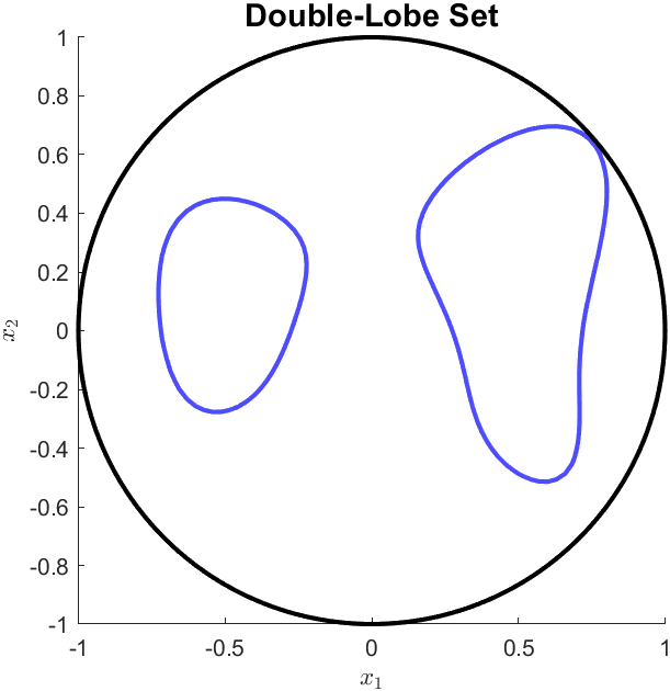
Figure 4: Double-lobe from (45)

Table 7: Double-Lobe without translation

Order	1	2	3	4	5	6
Indicator (18)	2.0	2.0	1.9118	1.9044	1.8270	1.5324
Stokes (42)	2.0	2.0	1.6322	1.5649	1.5256	1.0959

Table 8: Double-Lobe with translation

Order	1	2	3	4	5	6
Indicator (18)	2.0	2.0	1.9910	1.9833	1.8608	1.8294
Stokes (42)	2.0	2.0	1.9799	1.6123	1.5409	1.4728

7.3 Double Ellipsoid Cut

This experiment involves a three-dimensional region formed by the exclusion of two ellipsoids. This example is performed with $R=1$, such that $L$ has the constraint-definition of:

$$L=\begin{Bmatrix}x\in\mathbb{R}^{3}\mid\begin{array}[]{l}1-\lVert x\rVert_{2}^{2}\geq 0\\ x_{1}^{2}+4x_{2}^{2}+16x_{3}^{2}-1\geq 0\\ 3.25x_{1}^{2}-1.6700x_{1}x_{2}-1.9902x_{1}x_{3}+3.0703x_{2}^{2}-2.2158x_{2}x_{3}+2.6796x_{3}^{2}-1\geq 0\end{array}\end{Bmatrix}.$$ (46)

The geometry of the region $L$ is shown in Figure 5. The set $L$ is inside the gray sphere and outside the two ellipsoids.

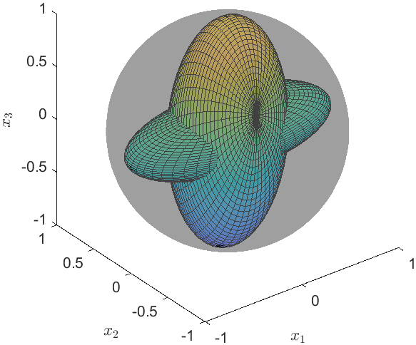
Figure 5: Visualization of double-ellipse-cut region in (46)

Table 9 reports on slice-volume bounds for the double-ellipse-cut region in (46) in which only translation in the direction $\theta=[1;0;0]$ is allowed (with $[\theta,Z]$ equal to the Identity matrix). The polynomials $(w,u)$ depend on the 3 variables $(t,y_{1},y_{2})$.

Table 9: Double-Ellipse-Cut with only translation

Order	4	5	6	7	8	9
Indicator (18)	3.1029	2.9132	2.8556	2.7739	2.6986	2.6653
Stokes (42)	2.8013	2.5739	2.2680	2.1333	2.1261	2.0814

Upper-bounds of the maximal slice-volume under pure rotation for the double-ellipse-cut set at orders $k\in\{1,2,3,4\}$ have values of $\pi$ (with and without Stokes constraints). Computational limitations on the experimental platform prevent the generation and solutions of SDPs (18) and (42) at order $k=4$.

8 Extensions

This section will detail extensions of the developed slice-volume program to other problems.

8.1 Radon Transform Maximization

Consider a (lower-semicontinuous) function $f(x)$ that is compactly supported over the ball $B_{R}^{n}$. The Radon-Transform supremization problem for $f$ is

Problem 4.

Find a direction $\theta$ and an affine offset $t$ to maximize

$$F^{*}= \sup_{\theta,t}\mathcal{R}f(\theta,t)$$ (47)

$$\theta\in S^{n},\ t\in[-R,R].$$

By using the support-set definition for $\Omega$ from (7a) and the method from Problem (61), we can formulate an LP to upper-bound (47) as

$$f^{*}= \inf_{\gamma\in\mathbb{R}}\quad\gamma$$ (48a)

$$\gamma\geq\Lambda_{R}w(\theta,t,Z) \forall(\theta,t)\in\Omega_{Z}$$ (48b)

$$w(\theta,t,Z,y)\geq f(\theta t+Zy) \forall(\theta,t,y,Z)\in\Psi$$ (48c)

$$w(\theta,t,Z,y)\in C(\Psi).$$ (48d)

Note that constraint (48c) is equivalent to the pair of (9c) and (9d) when $f=I_{L}$.

8.2 Radon Transform Approximation

The program in (61) aims to find the supremal slice volume of a set $L\subseteq B_{R}^{n}$. The produced auxiliary function $w$ produces an upper-bound $\int_{B_{R}^{n}}w(\theta,t,y)dy$ on the Radon transform $\mathcal{R}I_{L}$ (Theorem 3.3), but this tightness only needs to be satisfied at the critical $(\theta^{*},t^{*})$. We can also seek to develop a function that is as close to $\mathcal{R}I_{L}$ as possible in an $L_{1}$ sense, thus producing an outer-approximation for the Radon Transform.

$$J^{*}= \inf\int_{O(n)}\int_{[-R,R]}\int_{B_{R}^{n-1}}w_{R}(\theta,t,Z,y)dy\,dt\,(d\theta\,dZ)$$ (49a)

$$w_{R}(\theta,t,Z,y)\geq 1 \forall(\theta,t,y,Z)\in\Psi_{L}$$ (49b)

$$w_{R}(\theta,t,Z,y)\geq 0 \forall(\theta,t,Z,y)\in\Psi$$ (49c)

$$w_{R}(\theta,t,Z,y)\in C(\Psi).$$ (49d)

The objective in (49) integrates over all variables $(\theta,t,y,Z)$ to develop a maximally-tight approximation.

Problem (49) is closely linked to the study of intersection bodies. [72, 73]. The intersection body $K$ of a star-shaped set $L$ containing the origin is the unique set such that

$$K =\{y\in\mathbb{R}^{n}\mid\lVert y\rVert_{2}\leq\text{vol}((y\cdot x=0)\cap L)\}.$$ (50)

Equivalently, the radial function of the set $K$ is the slice-volume at normal $y/\lVert y\rVert_{2}$. Any degree-$k$ moment-SOS truncation of (49) with polynomial $w_{R}\in\mathbb{R}[\theta,t,y]_{\leq 2k}$ and $q_{R}=\int_{B_{R}^{n-1}}w_{R}(\theta,t,y)dy$ will satisfy

$$K\subseteq\{\theta t\mid(\theta,t)\in S^{n}\times[-R,R]:t\leq q(\theta,0)\},$$ (51)

thus outer-approximating the intersection body.

9 Conclusion

This work presented the slice-volume problem for compact semialgebraic sets. The slice-volume program was posed the infinite-dimensional primal-dual pair of LPs (9) and (15). These LPs have no relaxation gap to the original slice-volume task when a bound on $R$ is known (A1). The LPs can be approximated by the moment-SOS hierarchy of SDP, with convergence as the degree $k$ tends to infinity. The complexity of these large-scale SDPs were reduced by applying symmetry, algebraic structure, and topological properties (assignment of $Z$). Stokes constraints for volume computation were incorporated into the slice-volume framework, and the improved convergence of stokes constraints was empirically demonstrated in experiments.

Future work includes determining the convergence rate of the slice-volume scheme, providing conditions under which the infimal Stokes program (42) achieves a minimum, applying SAGBI bases [74, 75] to the continuous symmetry reductions in Section 5.1.2, and finding sets under which slice-volume computation has a simpler structure (such as the polytopes in [25]). Another research direction that this framework can be extended towards SOS-based analysis of more general integral transformations (such as the X-ray transform [1]). The computational complexity analysis in Sections 4.3 and 5 consider an SDP framework for polynomial optimization. Further complexity reduction could be obtained with the development of more efficient SDP solvers, or by utilizing non-SDP optimization strategies [76, 77] to solve the slice-volume problem. Other investigations include formulating and implementing these non-SOS algorithms for slice-volume optimization, such as by modifying the real-algebraic algorithm from [44].

Appendix A Strong Duality of Indicator Slice-Volume

This proof of strong duality between (9) and (15) will use notation conventions from Theorem 2.6 of [67].

A.1 Weak Duality

The variables of (9) and (15) may be expressed as

$$\boldsymbol{\ell} =(w,\gamma)$$ (52)

$$\boldsymbol{\mu} =(\mu_{0},\mu,\hat{\mu}).$$ (53)

The residing space of $\boldsymbol{\ell}$ is

$$\mathcal{Y}^{\prime} =C(\Psi)\times\mathbb{R}$$ (54)

$$\mathcal{Y} =\mathcal{M}(\Psi)\times\mathbb{R}.$$ (55)

The spaces for $\boldsymbol{\mu}$ are

$$\mathcal{X}^{\prime} =C(\Omega_{Z})\times C(\Psi_{L})\times C(\Psi)$$ (56)

$$\mathcal{X} =\mathcal{M}(\Omega_{Z})\times\mathcal{M}(\Psi_{L})\times\mathcal{M}(\Psi),$$

with nonnegative subcones of

$$\mathcal{X}^{\prime}_{+} =C_{+}(\Omega_{Z})\times C_{+}(\Psi_{L})\times C_{+}(\Psi)$$ (57)

$$\mathcal{X}_{+} =\mathcal{M}_{+}(\Omega_{Z})\times\mathcal{M}_{+}(\Psi_{L})\times\mathcal{M}_{+}(\Psi).$$

We will also follow convention with [67] and refer to $\mathcal{Y}^{\prime}_{+}=\mathcal{Y}^{\prime}$ and $\mathcal{Y}_{+}=\mathcal{Y}$, because there are conic inequalities present in the affine constraints. The feasible sets of (9) and (15) are $\boldsymbol{\ell}\in\mathcal{Y}^{\prime}$ and $\boldsymbol{\mu}\in\mathcal{X}_{+}$ respectively. Additionally, the compactness assumption A1 ensures that $(\mathcal{X}_{+},\mathcal{X}_{+}^{\prime})$ form a pair of topological dual spaces. The set $\mathcal{Y}^{\prime}$ is equipped with the sup-norm-bounded topology, and the set $\mathcal{X}$ possesses the weak-* topology.

An affine map $\mathcal{A}$ with adjoint $\mathcal{A}^{\prime}$ may be defined from the constraints of (15) as

$$\mathcal{A}(\boldsymbol{\mu}) =[\mu_{0}\otimes\lambda_{R}^{n-1}-\mu-\hat{\mu},\ \langle 1,\mu_{0}\rangle]$$ (58)

$$\mathcal{A}^{\prime}(\boldsymbol{\ell}) =[\gamma-\textstyle\Lambda_{R}w(\theta,t,y),w,w].$$

The cost and constraint terms of (15) can be expressed as

$$\mathbf{b} =[0,\ 1,\ 0]$$ (59a)

$$\mathbf{c} =[0,\ 0,\ 1].$$ (59b)

Pairing of the data in (59) with the variables in (53) yield the objectives of (9) and (15):

$$\langle\boldsymbol{\ell},\mathbf{b}\rangle =\gamma$$ (60a)

$$\langle\mathbf{c},\boldsymbol{\mu}\rangle =\langle 1,\mu\rangle.$$ (60b)

A standard-form expression for (9) is

$$p^{*}= \inf_{\boldsymbol{\ell}\in\mathcal{Y}^{\prime}_{+}}\langle\boldsymbol{\ell},\mathbf{b}\rangle \mathcal{A}^{\prime}(\boldsymbol{\ell})-\mathbf{c}\in\mathcal{X}_{+},$$ (61)

and the standard-form expression for (15) is

$$M^{*}= \sup_{\boldsymbol{\mu}\in\mathcal{X}_{+}}\langle\mathbf{c},\boldsymbol{\mu}\rangle \mathbf{b}-\mathcal{A}(\boldsymbol{\mu})\in\mathcal{Y}_{+}.$$ (62)

A.2 Strong Duality

Sufficient conditions for the strong duality of (61) and (62) by Theorem 2.6 of [67]) are:

• The feasible measure solutions of $\boldsymbol{\mu}\in\mathcal{X}_{+}:\mathcal{A}(\boldsymbol{\mu})\in\mathcal{Y}_{+}$ are bounded.

• There exists a bounded feasible $\boldsymbol{\mu}$.

• The vectors in (59) are continuous, and all functions used to describe $\mathcal{A}$ is also continuous.

Boundedness of measures is proven in Lemma 3.4, verifying R1. The proof of 3.3 outlines a procedure to obtain a feasible $\boldsymbol{\mu}$ from any $(\theta,t)\in\Omega$, fulfilling R2. Requirement R3 is also satisfied, given that the vectors in (59) are constant, and the mapping $w(t,\theta,Z,y)\mapsto\Lambda_{R}w(\theta,t,Z)$ is continuous in $(\theta,t)\in\Omega$ for every $w\in C(\Psi)$.

Strong duality between (9) and (15) is therefore proven.

Appendix B Polynomial Approximability

This appendix proves that $w(\theta,t,Z,y)$ in (9e) can be taken to be polynomial.

B.1 Preliminary Polynomial Approximation Lemmas

In order to prove SOS convergence of (18) with $\lim_{k\rightarrow\infty}p^{*}_{k}=P^{*}$, we require the following lemma ensuring that it is possible to approximate with polynomials:

Lemma B.1.

For any $\epsilon\geq 0$ and set $L$ respecting A1, there exists a polynomial $w^{p}\in\mathbb{R}[\theta,t,Z,y]$ such that $w^{p}>I_{\Psi_{L}}$ and $P^{*}+\epsilon\geq\sup_{(\theta,t,Z)\in\Omega_{Z}}\Lambda_{R}w^{p}(\theta,t,Z)>P^{*}$.

Proof.

Let $(w,\gamma)$ be any feasible solution to (9b)-(9d) such that $\gamma\geq P^{*}$. Letting $\eta>0$ be a tolerance, it therefore holds that $(w+\eta)$ is strictly feasible for (9c)-(9d). There exists a polynomial $w^{p}\in\mathbb{R}[\theta,t,Z,y]$ such that $\sup_{(\theta,t,Z,y)\in\Psi_{L}}\lvert w^{p}(\theta,t,Z,y)-(w(\theta,t,Z,y)+\eta)\rvert\leq\eta/2$ in the compact $\Psi_{L}$ (A1) by the Stone-Weierstrass theorem. As such, the polynomial $w^{p}$ is strictly feasible for (9c)-(9d).The integrals are therefore related by

$$\Lambda_{R}w^{p}(\theta,t,Z) \leq\Lambda_{R}(w(\theta,t,y)+\eta+\eta/2)$$ (63a)

$$=\Lambda_{R}(w(\theta,t,Z))+3\eta/2\textrm{Vol}_{B^{n-1}_{R}}$$ (63b)

$$\leq\gamma+3\eta/2\textrm{Vol}(B^{n-1}_{R}).$$ (63c)

It therefore holds that for each $\epsilon>0$, an $\eta>0$ can be chosen such that $\epsilon>3\eta/2\textrm{Vol}(B^{n-1}_{R})$. This approximation can become arbitrarily tight by letting $\epsilon,\eta\rightarrow 0$. ∎

Lemma B.2.

Under assumption A1 and A2, the sets $\Omega,$ $\Omega_{Z}$, $\Psi$, and $\Psi_{L}$ all are BSA sets with ball constraints.

Proof.

The set $\Omega$ satisfies a ball constraint, because the description of $\Omega$ includes the constraints $1-\lVert\theta\rVert_{2}^{2}\geq 0$ and $R^{2}-t^{2}\geq 0$. Therefore, $R_{1}=\sqrt{R^{2}+1}$ ensures that $R_{1}^{2}-\lVert\theta\rVert_{2}^{2}-t^{2}\in\Sigma[\Omega]$.

We now consider the set $\Omega_{Z}$, which includes the constraint $[\theta,\,Z]\in O(n)$. This orthogonality constraint implies that $\lVert\theta\rVert_{2}^{2}+\sum_{ij}Z_{ij}^{2}=n$. The set $\Psi_{L}$ is therefore ball-constrained with $R_{2}=\sqrt{2R^{2}+n}$ under $R_{2}^{2}-\lVert\theta\rVert_{2}^{2}-t^{2}-\lVert y\rVert_{2}^{2}-\sum_{ij}Z_{ij}^{2}\in\Sigma[\Psi_{L}]$. The set $\Psi$ is ball-constrained with $R_{3}=\sqrt{2R_{2}^{2}+1}$ and $R_{3}^{2}-\lVert\theta\rVert_{2}^{2}-t^{2}-\lVert y\rVert_{2}^{2}-\sum_{ij}Z_{ij}^{2}\in\Sigma[\Omega\times B_{R}^{n-1}]$. Given that $\Psi_{L}\subseteq\Psi$ (and the BSA representation of $\Psi_{L}$ contains all constraints of $\Psi$), it holds that $\Psi_{L}$ is also ball-constrained.

∎

B.2 Proof of Theorem 4.2

Lemma B.1 ensures that constraints (9b)-(9d) can be fulfilled strictly by polynomials. The Putinar Positivestellensatz [49] implies that every positive polynomial over a ball-constrained set is also WSOS. Ball-constraints for the sets of interest are verified by Lemma B.2. As such, increasing the degree $k$ sufficiently high will ensure that a feasible polynomial $w_{k}$ will be found for each $\epsilon>0$. Letting $\epsilon\rightarrow 0$ in the limit proves the validity of this theorem.

Appendix C Strong Duality of Stokes Slice-Volume

This appendix proves strong duality between (42) and (41). The structure of the weak duality portion will follow the format of Appendix A.

C.1 Weak Duality

The optimization variables of (42) and (41) are

$$\boldsymbol{\ell} =(w,\gamma,u)$$ (64)

$$\boldsymbol{\mu} =(\mu_{0},\mu,\hat{\mu},\{\nu_{i}\}_{i=1}^{N_{c}}).$$ (65)

The space containing $\boldsymbol{\ell}$ is

$$\mathcal{Y}^{\prime} =C(\Psi)\times\mathbb{R}\times(C^{1}(\Psi_{L}))^{n}$$ (66)

$$\mathcal{Y} =\mathcal{M}(\Psi)^{\prime}\times\mathbb{R}\times((C^{1}(\Psi_{L})^{\prime})^{n}.$$ (67)

The sets defining $\boldsymbol{\mu}$ are

$$\mathcal{X}^{\prime} =C(\Omega_{Z})\times C(\Psi_{L})\times C(\Psi)\times\prod_{i=1}^{N_{c}}C(\Psi_{L}^{i})$$ (68)

$$\mathcal{X} =\mathcal{M}(\Omega_{Z})\times\mathcal{M}(\Psi_{L})\times\mathcal{M}(\Psi)\times\prod_{i=1}^{N_{c}}\mathcal{M}(\Psi_{L}^{i}),$$

and their nonnegative subcones of

$$\mathcal{X}^{\prime}_{+} =C_{+}(\Omega_{Z})\times C_{+}(\Psi_{L})\times C_{+}(\Psi)\times\prod_{i=1}^{N_{c}}C_{+}(\Psi_{L}^{i})$$ (69)

$$\mathcal{X}_{+} =\mathcal{M}_{+}(\Omega_{Z})\times\mathcal{M}_{+}(\Psi_{L})\times\mathcal{M}_{+}(\Psi)\prod_{i=1}^{N_{c}}\mathcal{M}_{+}(\Psi_{L}^{i}).$$

The convention of $\mathcal{Y}^{\prime}_{+}=\mathcal{Y}^{\prime}$ and $\mathcal{Y}_{+}=\mathcal{Y}$ is maintained, resulting in feasible set expressions of $\boldsymbol{\ell}\in\mathcal{Y}^{\prime}$ and $\boldsymbol{\mu}\in\mathcal{X}_{+}$ for (42) and (41).

We define an affine map $\mathcal{A}$ and its adjoint $\mathcal{A}^{\prime}$ from (41) with

$$\mathcal{A}(\boldsymbol{\mu}) =[\mu_{0}\otimes\lambda_{R}^{n-1}-\mu-\hat{\mu},\ \langle 1,\mu_{0}\rangle,\ [\text{grad}_{y}]_{G}\mu-\textstyle\sum_{i=1}^{L}[\text{grad}_{y}(\theta t+Zy)_{\#}g_{i}]_{G}\nu_{i}]$$ (70)

$$\mathcal{A}^{*}(\boldsymbol{\ell}) =[\gamma-\textstyle\Lambda_{R}w(\theta,t,Z),\ w-[\nabla_{y}\cdot u]_{G},w,\ -[u\cdot\nabla_{y}g_{i}]_{G}],$$

and also set the cost and constraint vectors of (41) as

$$\mathbf{b} =[0,\ 1,\ 0,\mathbf{0}_{n}]$$ (71a)

$$\mathbf{c} =[0,\ 0,\ 1,\mathbf{0}_{N_{c}}],$$ (71b)

to form the following pairings:

$$\langle\boldsymbol{\ell},\mathbf{b}\rangle =\gamma$$ (72a)

$$\langle\mathbf{c},\boldsymbol{\mu}\rangle =\langle 1,\mu\rangle.$$ (72b)

Under these definitions, the Stokes measure program in (41) is therefore

$$m^{*}_{s}= \sup_{\boldsymbol{\mu}\in\mathcal{X}_{+}}\langle\mathbf{c},\boldsymbol{\mu}\rangle \mathbf{b}-\mathcal{A}(\boldsymbol{\mu})\in\mathcal{Y}_{+}.$$ (73)

and the function program (42) is

$$p^{*}_{s}= \inf_{\boldsymbol{\ell}\in\mathcal{Y}^{\prime}_{+}}\langle\boldsymbol{\ell},\mathbf{b}\rangle \mathcal{A}^{\prime}(\boldsymbol{\ell})-\mathbf{c}\in\mathcal{X}_{+}.$$ (74)

Weak duality implies that $p^{*}_{s}\geq m^{*}_{s}$.

C.2 Strong Duality

We assemble a set of relations between optimal values under A1-A4:

Table 10: LP optimality relations to prove Stokes strong duality

$m^{*}_{s}=m^{*}$	Theorem 6.4
$m^{*}=p^{*}$	Theorem 3.5
$p^{*}\geq p^{*}_{s}$	Proposition 6.5
$p^{*}_{s}\geq m^{*}_{s}$	Weak duality (Stokes)

Table 10 results in the sandwich of $p^{*}\leq p^{*}_{s}\leq m^{*}_{s}$. Given that $m^{*}_{s}=m^{*}=p^{*}$, it therefore holds that the strong duality relation of $m^{*}_{s}=p^{*}_{s}$ is proven.

References

- [1] S. Helgason and S. Helgason, The Radon Transform. Springer, 1980, vol. 2.
- [2] R. J. Gardner, Geometric Tomography, 2nd ed., ser. Encyclopedia of Mathematics and its Applications. Cambridge University Press, New York, 2006, vol. 58.
- [3] ——, “Intersection bodies and the Busemann-Petty problem,” Trans. Amer. Math. Soc., vol. 342, no. 1, pp. 435–445, 1994. [Online]. Available: https://doi.org/10.2307/2154703
- [4] ——, “A positive answer to the Busemann-Petty problem in three dimensions,” Ann. of Math. (2), vol. 140, no. 2, pp. 435–447, 1994. [Online]. Available: https://doi.org/10.2307/2118606
- [5] A. Koldobsky, “Intersection bodies, positive definite distributions, and the Busemann-Petty problem,” Amer. J. Math., vol. 120, no. 4, pp. 827–840, 1998.
- [6] R. J. Gardner, A. Koldobsky, and T. Schlumprecht, “An analytic solution to the Busemann-Petty problem on sections of convex bodies,” Ann. of Math. (2), vol. 149, no. 2, pp. 691–703, 1999. [Online]. Available: https://doi.org/10.2307/120978
- [7] G. Zhang, “A positive solution to the Busemann-Petty problem in ,” Ann. of Math. (2), vol. 149, no. 2, pp. 535–543, 1999. [Online]. Available: https://doi.org/10.2307/120974
- [8] B. Klartag and V. Milman, “The Slicing Problem by Bourgain,” in Analysis at Large: Dedicated to the Life and Work of Jean Bourgain, A. Avila, M. T. Rassias, and Y. Sinai, Eds. Cham: Springer International Publishing, 2022, pp. 203–231.
- [9] B. Klartag and J. Lehec, “Bourgain’s slicing problem and KLS isoperimetry up to polylog,” Geom. Funct. Anal., vol. 32, no. 5, pp. 1134–1159, 2022.
- [10] B. Klartag, “Logarithmic bounds for isoperimetry and slices of convex sets,” 2023.
- [11] A. Giannopoulos, A. Koldobsky, and A. Zvavitch, “Inequalities for sections and projections of convex bodies,” 2023.
- [12] S. Webb, “Central slices of the regular simplex,” Geom. Dedicata, vol. 61, no. 1, pp. 19–28, 1996.
- [13] H. König, “Non-central sections of the simplex, the cross-polytope and the cube,” Adv. Math., vol. 376, pp. Paper No. 107 458, 35, 2021.
- [14] D. W. Walkup, “A simplex with a large cross section,” Amer. Math. Monthly, vol. 75, pp. 34–36, 1968.
- [15] K. Ball, “Cube slicing in ,” Proc. Amer. Math. Soc., vol. 97, no. 3, pp. 465–473, 1986.
- [16] ——, “Volumes of sections of cubes and related problems,” in Geometric aspects of functional analysis (1987–88), ser. Lecture Notes in Math. Springer, Berlin, 1989, vol. 1376, pp. 251–260.
- [17] J. Lawrence, “Cutting the -cube,” J. Res. Nat. Bur. Standards, vol. 84, no. 1, pp. 51–53 (1978), 1979.
- [18] L. Pournin, “Shallow sections of the hypercube,” Israel Journal of Mathematics, 11 2022.
- [19] H. Fukuda, N. Muto, K. Goto, and G. Nakamura, “Sections of hyper-cube in five dimensions,” Forma, vol. 12, no. 1, pp. 15–33, 1997.
- [20] J. Moody, C. Stone, D. Zach, and A. Zvavitch, “A remark on the extremal non-central sections of the unit cube,” in Asymptotic geometric analysis, ser. Fields Inst. Commun. Springer, New York, 2013, vol. 68, pp. 211–228.
- [21] R. Liu and T. Tkocz, “A note on the extremal non-central sections of the cross-polytope,” Adv. in Appl. Math., vol. 118, pp. 102 031, 17, 2020.
- [22] M. Meyer and A. Pajor, “Sections of the unit ball of ,” J. Funct. Anal., vol. 80, no. 1, pp. 109–123, 1988.
- [23] A. Khovanskii, “Combinatorics of sections of polytopes and Coxeter groups in Lobachevsky spaces,” in The Coxeter legacy. Amer. Math. Soc., Providence, RI, 2006, pp. 129–157.
- [24] K. Berlow, M.-C. Brandenburg, C. Meroni, and I. Shankar, “Intersection bodies of polytopes,” Beiträge zur Algebra und Geometrie. Contributions to Algebra and Geometry, vol. 63, no. 2, pp. 419–439, 2022.
- [25] M.-C. Brandenburg, J. A. D. Loera, and C. Meroni, “The best ways to slice a polytope,” 2023.
- [26] L. Lovász and S. Vempala, “Simulated annealing in convex bodies and an o*(n4) volume algorithm,” Journal of Computer and System Sciences, vol. 72, no. 2, pp. 392–417, 2006.
- [27] A. Isaac, A. Jawlekar, and M. Venkatapathi, “An algorithm for estimating non-convex volumes and other integrals in n dimensions,” Computational and Applied Mathematics, vol. 42, no. 6, pp. 1–17, 2023.
- [28] M. E. Dyer and A. M. Frieze, “On the complexity of computing the volume of a polyhedron,” SIAM Journal on Computing, vol. 17, no. 5, pp. 967–974, 1988.
- [29] P. A. Parrilo, Structured semidefinite programs and semialgebraic geometry methods in robustness and optimization. California Institute of Technology, 2000.
- [30] J. B. Lasserre, Moments, Positive Polynomials And Their Applications, ser. Imperial College Press Optimization Series. World Scientific Publishing Company, 2009.
- [31] D. Henrion, J. B. Lasserre, and C. Savorgnan, “Approximate volume and integration for basic semialgebraic sets,” SIAM review, vol. 51, no. 4, pp. 722–743, 2009.
- [32] M. Tacchi, T. Weisser, J. B. Lasserre, and D. Henrion, “Exploiting sparsity for semi-algebraic set volume computation,” Foundations of Computational Mathematics, pp. 1–49, 2022.
- [33] C. Schlosser, M. Tacchi, and A. Lazarev, “Convergence rates for the moment-sos hierarchy,” arXiv preprint arXiv:2402.00436, 2024.
- [34] M. Korda and D. Henrion, “Convergence rates of moment-sum-of-squares hierarchies for volume approximation of semialgebraic sets,” Optimization Letters, vol. 12, pp. 435–442, 2018.
- [35] J. B. Lasserre, “Computing Gaussian & exponential measures of semi-algebraic sets,” Advances in Applied Mathematics, vol. 91, pp. 137–163, 2017.
- [36] M. Tacchi, J. B. Lasserre, and D. Henrion, “Stokes, Gibbs, and Volume Computation of Semi-Algebraic Sets,” Discrete & Computational Geometry, vol. 69, no. 1, pp. 260–283, 2023.
- [37] J. B. Lasserre and V. Magron, “Computing the Hausdorff boundary measure of semialgebraic sets,” SIAM Journal on Applied Algebra and Geometry, vol. 4, no. 3, pp. 441–469, 2020.
- [38] D. Henrion and M. Korda, “Convex computation of the region of attraction of polynomial control systems,” IEEE Trans. Automat. Contr., vol. 59, no. 2, p. 297–312, Feb 2014.
- [39] A. Majumdar, R. Vasudevan, M. M. Tobenkin, and R. Tedrake, “Convex Optimization of Nonlinear Feedback Controllers via Occupation Measures,” The International Journal of Robotics Research, vol. 33, no. 9, pp. 1209–1230, 2014.
- [40] M. Korda, D. Henrion, and C. N. Jones, “Inner approximations of the region of attraction for polynomial dynamical systems,” IFAC Proceedings Volumes, vol. 46, no. 23, pp. 534–539, 2013.
- [41] A. Oustry, M. Tacchi, and D. Henrion, “Inner approximations of the maximal positively invariant set for polynomial dynamical systems,” IEEE Control Systems Letters, vol. 3, no. 3, pp. 733–738, 2019.
- [42] M. Korda, D. Henrion, and C. N. Jones, “Convex computation of the maximum controlled invariant set for polynomial control systems,” SIAM Journal on Control and Optimization, vol. 52, no. 5, pp. 2944–2969, 2014.
- [43] C. Schlosser and M. Korda, “Converging outer approximations to global attractors using semidefinite programming,” Automatica, vol. 134, p. 109900, 2021.
- [44] P. Lairez, M. Mezzarobba, and M. Safey El Din, “Computing the volume of compact semi-algebraic sets,” in Proceedings of the 2019 on International Symposium on Symbolic and Algebraic Computation, 2019, pp. 259–266.
- [45] T. Oaku, “Algorithms for integrals of holonomic functions over domains defined by polynomial inequalities,” Journal of Symbolic Computation, vol. 50, pp. 1–27, 2013.
- [46] A. Barvinok, A Course in Convexity. American Mathematical Society, 2002.
- [47] T. Tao, An Introduction to Measure Theory. American Mathematical Society Providence, RI, 2011, vol. 126.
- [48] D. Hilbert, “Über die Darstellung definiter Formen als Summe von Formenquadraten,” Mathematische Annalen, vol. 32, no. 3, pp. 342–350, 1888.
- [49] M. Putinar, “Positive Polynomials on Compact Semi-algebraic Sets,” Indiana University Mathematics Journal, vol. 42, no. 3, pp. 969–984, 1993.
- [50] J. Nie and M. Schweighofer, “On the complexity of Putinar’s Positivstellensatz,” Journal of Complexity, vol. 23, no. 1, pp. 135–150, 2007.
- [51] J. Cimprič, M. Marshall, and T. Netzer, “Closures of quadratic modules,” Israel Journal of Mathematics, vol. 183, no. 1, pp. 445–474, 2011.
- [52] J. Guthrie, “Inner and outer approximations of star-convex semialgebraic sets,” IEEE Control Systems Letters, vol. 7, pp. 61–66, 2022.
- [53] D. Gottlieb and C.-W. Shu, “On the Gibbs phenomenon and its resolution,” SIAM review, vol. 39, no. 4, pp. 644–668, 1997.
- [54] R. B. Ash, Real analysis and probability: probability and mathematical statistics: a series of monographs and textbooks. Academic press, 1972.
- [55] D. Henrion and J.-B. Lasserre, “Inner Approximations for Polynomial Matrix Inequalities and Robust Stability Regions,” IEEE Transactions on Automatic Control, vol. 57, no. 6, pp. 1456–1467, 2011.
- [56] J. B. Lasserre and E. S. Zeron, “Solving a class of multivariate integration problems via laplace techniques,” Applicationes Mathematicae, vol. 28, pp. 391–405, 2001.
- [57] D. Henrion and J.-B. Lasserre, “Detecting global optimality and extracting solutions in gloptipoly,” in Positive polynomials in control. Springer, 2005, pp. 293–310.
- [58] J. Miller, T. Dai, and M. Sznaier, “Data-Driven Superstabilizing Control of Error-in-Variables Discrete-Time Linear Systems,” in 2022 61st IEEE Conference on Decision and Control (CDC), 2022, pp. 4924–4929.
- [59] K. Gatermann and P. A. Parrilo, “Symmetry groups, semidefinite programs, and sums of squares,” Journal of Pure and Applied Algebra, vol. 192, no. 1-3, pp. 95–128, 2004.
- [60] J. Lofberg, “Pre-and post-processing sum-of-squares programs in practice,” IEEE transactions on automatic control, vol. 54, no. 5, pp. 1007–1011, 2009.
- [61] D. Cox, J. Little, and D. OShea, Ideals, varieties, and algorithms: an introduction to computational algebraic geometry and commutative algebra. Springer Science & Business Media, 2013.
- [62] P. A. Parrilo, “Exploiting structure in sum of squares programs,” in 42nd IEEE International Conference on Decision and Control (IEEE Cat. No. 03CH37475), vol. 5. IEEE, 2003, pp. 4664–4669.
- [63] ——, “Exploiting algebraic structure in sum of squares programs,” in Positive polynomials in control. Springer, 2005, pp. 181–194.
- [64] R. Bott and J. Milnor, “On the parallelizability of the spheres,” Bulletin of the American Mathematical Society, vol. 64, no. 3.P1, pp. 87 – 89, 1958.
- [65] H. Whitney, Geometric Integration Theory. Courier Corporation, 2012.
- [66] J. Harrison, “Flux across nonsmooth boundaries and fractal Gauss/Green/Stokes’ theorems,” Journal of Physics A: Mathematical and General, vol. 32, no. 28, p. 5317, 1999.
- [67] M. Tacchi, “Moment-SOS hierarchy for large scale set approximation. application to power systems transient stability analysis,” Ph.D. dissertation, Toulouse, INSA, 2021.
- [68] C. Riener, T. Theobald, L. J. Andrén, and J. B. Lasserre, “Exploiting symmetries in sdp-relaxations for polynomial optimization,” Mathematics of Operations Research, vol. 38, no. 1, pp. 122–141, 2013.
- [69] J. Wang, V. Magron, J. B. Lasserre, and N. H. A. Mai, “CS-TSSOS: Correlative and term sparsity for large-scale polynomial optimization,” ACM Transactions on Mathematical Software, vol. 48, no. 4, pp. 1–26, 2022.
- [70] M. Lubin, O. Dowson, J. D. Garcia, J. Huchette, B. Legat, and J. P. Vielma, “JuMP 1.0: Recent improvements to a modeling language for mathematical optimization,” Mathematical Programming Computation, 2023.
- [71] M. ApS, The MOSEK optimization toolbox for MATLAB manual. Version 10.1., 2023.
- [72] R. J. Gardner, “Intersection bodies and the Busemann-Petty problem,” Transactions of the American Mathematical Society, vol. 342, no. 1, pp. 435–445, 1994.
- [73] K. Berlow, M.-C. Brandenburg, C. Meroni, and I. Shankar, “Intersection bodies of polytopes,” Beiträge zur Algebra und Geometrie / Contributions to Algebra and Geometry, vol. 63, no. 2, pp. 419–439, jan 2022.
- [74] L. Robbiano and M. Sweedler, “Subalgebra bases,” in Commutative Algebra: Proceedings of a Workshop held in Salvador, Brazil, Aug. 8–17, 1988. Springer, 2006, pp. 61–87.
- [75] M. Stillman and H. Tsai, “Using sagbi bases to compute invariants,” Journal of Pure and Applied Algebra, vol. 139, no. 1-3, pp. 285–302, 1999.
- [76] D. Papp and S. Yildiz, “Sum-of-Squares Optimization without Semidefinite Programming,” SIAM Journal on Optimization, vol. 29, no. 1, pp. 822–851, 2019.
- [77] S. Cristancho and M. Velasco, “Harmonic hierarchies for polynomial optimization,” arXiv preprint arXiv:2202.12865, 2022.