Wavepacket interference of two photons: from temporal entanglement to wavepacket shaping

Abstract

Quantum interference based on beam splitting can be used for entanglement generations and has applications in quantum information. However, interference among photons with different temporal shapes has received little attention. Here we analytically study the interference of two photons with different temporal shapes through a beam splitter (BS), and propose its application in temporal entanglement and shaping of photons. The temporal entanglement is determined by the splitting ratio of BS and temporal indistinguishability of input photons. Maximum entanglement can be achieved with a 50/50 BS configuration. Then, detecting one of the entangled photons at a specific time enables the probabilistic shaping of the other photon. This process can shape the exponentially decaying (ED) wavepacket into the ED sine shapes, which can be further shaped into Gaussian shapes with fidelity exceeding 99%. The temporal entanglement and shaping of photons based on interference may solve the shape mismatch issues in complex large-scale optical quantum networks.

I Introduction

The non-classical interference processes among photons based on beam splitting are essential for both fundamental physics [1] and applications in quantum information [2, 3]. Present researches on quantum interference primarily concentrate on identical photons, while the fruitful information on partially indistinguishable photons with different temporal shapes, has not been fully recognized. Over the past decades, researches have demonstrated that temporal entanglement can be realized through the wavepacket interference of photons [4, 5, 6]. Based on time-resolved measurements, quantum beat patterns on correlation functions have been theoretically predicted [7, 8] and experimentally demonstrated [9, 10]. However, until now, a comprehensive and quantitative description of the temporal entanglement generated through wavepacket interference is lacking. Furthermore, the modulation of the temporal entanglement based on beam splitting remains elusive.

The temporal shape of photons also plays a crucial role in the light-matter interactions [11, 12, 13, 14], deterministic quantum state transfer [15] and implementation of quantum logic gates [16]. Therefore, shaping the wavepacket of photons on demand has emerged as a pivotal aspect of quantum photonics. Current methods for shaping the photons include manipulating the emission of the quantum emitters dynamically [15] or passively [17], direct phase modulation [18, 19], spectral filtering [20], and manipulating one of the entangled photon pairs [21, 22]. Nevertheless, shaping photons based on the wavepacket interference of photons via beam splitting remains unexplored.

In this research, we study the interference of two photon wavepackets with different temporal shapes through a beam splitter (BS). The two initially temporally separable photons become entangled after passing through the BS. We employ Schmidt decomposition approach to analyze the entanglement entropy, the measure of entanglement for output state are obtained. The entanglement degree of the output state components are determined by the photon temporal indistinguishability factor and splitting ratio of BS. By utilizing this entanglement and detecting one of the entangled photons at a specific time, temporal shaping of the other photon can be probabilistically achieved in a heralded way. There are two exact examples: (1) the exponentially decaying (ED) wavepacket can be shaped into the ED sine shapes and (2) the ED sine can be further shaped into Gaussian shapes with fidelity higher than 99%. The temporal entanglement and shaping of photons based on interference may address the shape mismatch issues in complex large-scale optical quantum networks.

II Analytical expression of the output state

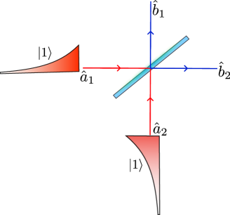
Figure 1: Schematic for the wavepacket interference of two photons through a beam splitter.

As shown in Fig. 1, we consider the interference of two photons with different temporal shapes through a two-port BS. The input state is a two-mode Fock state

$$|\psi_{\text{in}}\rangle=\int f_{1}\left(\tau_{1}\right)\hat{a}_{1}^{\dagger}\left(\tau_{1}\right)d\tau_{1}\int f_{2}\left(\tau_{2}\right)\hat{a}_{2}^{\dagger}\left(\tau_{2}\right)d\tau_{2}|0,0\rangle,$$ (1)

where $f_{n}(\tau_{n})$ is the temporal shape of the single photon wavepacket in the $n$-th input port of BS and satisfies the normalization condition $\int|f_{n}(\tau)|^{2}d\tau=1$, and $\hat{a}^{\dagger}_{n}(\tau)$ ($\hat{a}_{n}(\tau)$) is the continuous time creation (annihilation) operator [23]. The states in the output port of BS are defined by the operators $\hat{b}_{1/2}(\tau)$. The commutation relations of these continuous mode operators are $[\hat{a}_{n}(\tau_{1}),\hat{a}^{\dagger}_{n}(\tau_{2})]=\delta(\tau_{1}-\tau_{2}),\quad[\hat{b}_{n}(\tau_{1}),\hat{b}^{\dagger}_{n}(\tau_{2})]=\delta(\tau_{1}-\tau_{2})$. The linear relationship between the operators in the input and output ports can be described by the scattering matrix $\left(\begin{array}[]{c}\hat{b}_{1}(\tau)\\ \hat{b}_{2}(\tau)\end{array}\right)=\left(\begin{array}[]{cc}t&r\\ -r&t\end{array}\right)\left(\begin{array}[]{c}\hat{a}_{1}(\tau)\\ \hat{a}_{2}(\tau)\end{array}\right)$. Here $t,r$ are the transmission and reflection coefficients of BS. For convenience, we set $t$ and $r$ to be real numbers. For a lossless BS, $t^{2}+r^{2}=1$. After passing through the BS, the output state could be expressed as

$$|\psi_{\text{out}}\rangle=\sqrt{P_{0,2}}|0,2\rangle+\sqrt{P_{1,1}}|1,1\rangle+\sqrt{P_{2,0}}|2,0\rangle,$$ (2)

which means that there are three possible outcomes. Here $|m,2-m\rangle$ denotes the outcome with $m$ photons in the output port 1 and $2-m$ photons in the output port 2 of BS. $P_{m,2-m}$ denotes the probabilities of different outcomes and can be expressed as

$$\begin{split}&P_{2,0}=P_{0,2}=t^{2}r^{2}\left(1+|J|^{2}\right),\end{split}$$ (3a)

$$\begin{split}&P_{1,1}=(t^{2}-r^{2})^{2}+t^{2}r^{2}(1-|J|^{2}),\end{split}$$ (3b)

where $J=\int f_{1}(\tau)\left(f_{2}\right){}^{*}(\tau)\,d\tau$ is the temporal indistinguishability factor between the two input photons. $|J|=1$ indicates perfect photon indistinguishability and $|J|=0$ indicates the two photons are completely distinguishable. Therefore, the probability of each outcome is solely determined by the photon indistinguishability factor and splitting ratio of BS. The components $|0,2\rangle,|1,1\rangle,|2,0\rangle$ are expressed as follows

$$\begin{split}|0,2\rangle&\equiv\iint F_{0,2}\left(\tau_{1},\tau_{2}\right)\frac{\hat{b}_{2}^{\dagger}\left(\tau_{1}\right)\hat{b}_{2}^{\dagger}\left(\tau_{2}\right)}{\sqrt{2}}d\tau_{1}d\tau_{2}|0,0\rangle,\end{split}$$ (4a)

$$\begin{split}|1,1\rangle&\equiv\iint F_{1,1}\left(\tau_{1},\tau_{2}\right)\hat{b}_{1}^{\dagger}\left(\tau_{1}\right)\hat{b}_{2}^{\dagger}\left(\tau_{2}\right)d\tau_{1}d\tau_{2}|0,0\rangle,\end{split}$$ (4b)

$$\begin{split}|2,0\rangle&\equiv\iint F_{2,0}\left(\tau_{1},\tau_{2}\right)\frac{\hat{b}_{1}^{\dagger}\left(\tau_{1}\right)\hat{b}_{1}^{\dagger}\left(\tau_{2}\right)}{\sqrt{2}}d\tau_{1}d\tau_{2}|0,0\rangle,\end{split}$$ (4c)

where $F_{2,0}(\tau_{1},\tau_{2})=-F_{0,2}(\tau_{1},\tau_{2})=rt[f_{1}\left(\tau_{1}\right)f_{2}\left(\tau_{2}\right)+f_{2}\left(\tau_{1}\right)f_{1}\left(\tau_{2}\right)]/\sqrt{P_{2,0}}$, and $F_{1,1}(\tau_{1},\tau_{2})=[t^{2}f_{1}\left(\tau_{1}\right)\allowbreak f_{2}\left(\tau_{2}\right)-\allowbreak r^{2}f_{2}\left(\tau_{1}\right)f_{1}\left(\tau_{2}\right)]/\sqrt{P_{1,1}}$. Here $F_{m,2-m}(\tau_{1},\tau_{2})$ denotes the temporal shape or wavefunction of the part $|m,2-m\rangle$ and satisfies the normalization condition $\iint|F_{m,2-m}(\tau_{1},\tau_{2})|^{2}d\tau_{1}d\tau_{2}=1$.

The temporal shape of the output state includes the coherent superposition of the temporal shapes $f_{n}(\tau)$, making the two initially temporally separable photons become inseparable and entangled after passing through the BS. In fact, there are two kind of mechanisms resulting in the superposition of temporal shapes, both of which can be summarized as indistinguishability.

The first mechanism is the indistinguishability of photons as bosons in the same spatial mode, which results in the superposition of temporal shapes for the components $|2,0\rangle,|0,2\rangle$. For the outcome where the two photons are in the same output port, the wavefunctions need to satisfy the permutation symmetry due to the indistinguishability of photons as bosons, i.e., $F_{2,0}(\tau_{1},\tau_{2})=F_{2,0}(\tau_{2},\tau_{1})$, $F_{0,2}(\tau_{1},\tau_{2})=F_{0,2}(\tau_{2},\tau_{1})$. Consequently, the wavefunctions $F_{2,0}(\tau_{1},\tau_{2})$, $F_{0,2}(\tau_{1},\tau_{2})$ take the form of a superposition of multiple direct product wavefunctions $f_{n}(\tau)$ with equal coefficients.

The second mechanism is the indistinguishability of different photon pathways, which results in the superposition of temporal shapes for the component $|1,1\rangle$. That is, the physical process when two photons are either both reflected or both transmitted by BS is indistinguishable to some extent, they will result in the same photon number distribution outcome $|1,1\rangle$. The indistinguishability of photon pathways can be characterized by the transmission and reflection coefficients of BS as $\mathcal{P}=t^{2}-r^{2}$. Perfect indistinguishability of the photon pathways needs $\mathcal{P}=0$ which means that $t^{2}=r^{2}=1/2$. The superposition coefficient at this time is related to the transmission coefficients of BS.

In the next section, we will further show that in the wavepacket interference of two photons, the photon temporal intdistinguishability (J) and photon pathway indistinguishability ($\mathcal{P}$) are the two key factors in the temporal entanglement generations.

III Temporal entanglement of the output state

The analytical expressions provided in Eq. (4) reveal that the temporal shapes of different components $|m,2-m\rangle$ are different, leading to distinct entanglement characteristics. Prior studies have primarily concentrated on measuring the joint spectral density (JSD) profile [9, 24, 10, 8, 25], specifically focusing on the entanglement of the outcome $|1,1\rangle$. Here we give a comprehensive examination of the entanglement across all three potential outcomes by performing the Schmidt decomposition of their wavefunctions [26]

$$F_{m,2-m}(\tau_{1},\tau_{2})=\sum_{n=1}^{N}\lambda_{n}^{m}\phi_{n}^{m}\left(\tau_{1}\right)\tilde{\phi}_{n}^{m}\left(\tau_{2}\right),$$ (5)

which represents a weighted sum of products of $N$ orthogonal single-photon wavefunctions $\phi_{n}^{m}(\tau)$ and $\tilde{\phi}^{m}_{n}(\tau)$. The Schmidt modes $\phi_{n}^{m}(\tau)$ and $\tilde{\phi}_{n}^{m}(\tau)$ don’t necessarily to be orthogonal. The decomposition coefficients satisfy the normalization condition $\sum_{n}^{N}|\lambda_{n}^{m}|^{2}=1$. The Schmidt-mode single photon wavefunctions $\phi_{n}^{m}(\tau),\tilde{\phi}^{m}_{n}(\tau)$ form a complete set of orthogonal functions $\int\phi_{i}^{m*}(\tau)\phi_{j}^{m}(\tau)d\tau=\delta_{i,j},\int\tilde{\phi}_{i}^{m*}(\tau)\tilde{\phi}^{m}_{j}(\tau)d\tau=\delta_{i,j}$. For wavefunctions $F_{2,0}(\tau_{1},\tau_{2})$ , due to the permutation symmetry $F_{2,0}(\tau_{1},\tau_{2})=F_{2,0}(\tau_{2},\tau_{1})$, this leads to $\phi_{n}^{2}(\tau)=\tilde{\phi}_{n}^{2}(\tau),\phi_{n}^{2}(\tau)=\tilde{\phi}_{n}^{2}(\tau)$. If there is only one non-zero Schmidt coefficient, it implies that the two-photon wavefunction is separable, and the photons are not entangled. Otherwise, the two photons are temporally entangled. It should be noted that the meaning of entanglement we discussed here is suitable for two spatially separated photon. So, when mentioning the entanglement for Fock states components $|2,0\rangle$ and $|0,2\rangle$ in this work, we mean the two photon have been split by another 50/50 BS. In general, performing the Schmidt decomposition involves numerically calculating the eigenvalues and eigenfunctions of the corresponding temporal correlation matrix [26]. Following the expression in Eq. (4), where the temporal shape of the output state encompasses the coherent superposition of $f_{n}(\tau)$, the Schmidt decomposition can be analytically performed (See Appendix A). We derived that the wavefunctions of different parts can be decomposed as a superposition of two orthogonal Schmidt modes and the decomposition coefficients are

$$\begin{split}&|\lambda^{1}_{1,2}|^{2}=\frac{\left[\mathcal{P}^{2}+\frac{1}{2}\mathcal{J}^{2}\left(\mathcal{P}^{2}-1\right)\pm\mathcal{P}\sqrt{|J|^{2}\mathcal{J}^{2}(\mathcal{P}-1)^{2}+\left(-\mathcal{J}^{2}(-1+\mathcal{P})+\mathcal{P}\right)^{2}}\right]}{2(\mathcal{P}^{2}-\frac{1}{2}\mathcal{J}^{2}\left(-1+\mathcal{P}^{2}\right))},\end{split}$$ (6a)

$$\begin{split}&|\lambda^{0}_{1,2}|^{2}=|\lambda^{2}_{1,2}|^{2}=\frac{(1\pm|J|)^{2}}{2(1+|J|^{2})},\end{split}$$ (6b)

where $\mathcal{J}=\sqrt{1-|J|^{2}}$. Eq. (6) tells us that the Schmidt coefficients of the part $|2,0\rangle$ and $|0,2\rangle$ are equal which only related to the photon indistinguishability factor $J$, but the Schmidt coefficients of the part $|1,1\rangle$ are determined by both the photon indistinguishability $J$ and photon pathways indistinguishability $\mathcal{P}$. We take the wavepacket interference of two photons with different ED shapes as an example. By comparing with numerical results, we validate the correctness of our analytically derived Schmidt decomposition results (See Appendix B).

As an exact measure of entanglement, we also employ the Von Neumann entropy $\mathcal{S}$, which can be expressed in terms of Schmidt coefficients as

$$\mathcal{S}_{|m,2-m\rangle}=-\sum_{i=1}^{2}|\lambda_{i}^{m}|^{2}\log_{2}|\lambda_{i}^{m}|^{2}.$$ (7)

For entangled states $\mathcal{S}>0$. If $\mathcal{S}=0$ then the quantum state is separable. The maximum entanglement $\mathcal{S}=1$ is achieved when the two Schmidt mode coefficients are equal, signifying the realization of a two-photon Bell state encoded in the temporal mode.

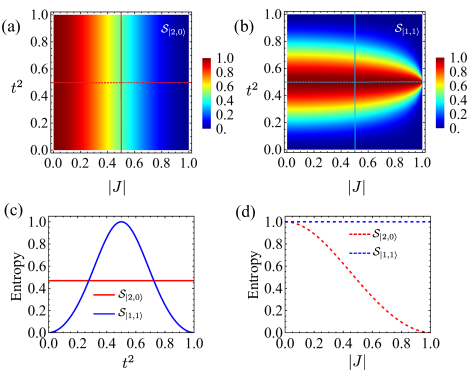
Figure 2: Von Neumann entropy of the output state for the outcome (a) $|1,1\rangle$ and (b) $|2,0\rangle$ as a function of photon indistinguishability and transmission of BS; Slice of the Von Neumann entropy of the outcome $|1,1\rangle$ (blue line) and $|2,0\rangle$ (red line) (c) as a function transmission of BS (solid line) when $|J|=0.5$ and (d) as a function photon indistinguishability (dashed line) when $t^{2}=0.5$.

We systematically investigate the effect of photon indistinguishability $|J|$ and transmission $t^{2}$ of BS on the Von Neumann entropy of the component $|1,1\rangle$ and $|2,0\rangle$. The results are depicted in Fig. 2(a) and (b), respectively. Fig. 2(c) and (d) are slice cuts of Von Neumann entropy along $|J|=0.5$ and $t^{2}=0.5$, respectively. Excepting the case that $t^{2}=0.5$, a common feature is that as the increase of the photon indistinguishability $|J|$, the temporal entanglement of the component $|1,1\rangle$ and $|2,0\rangle$ will both decrease. In conventional HOM interference, perfect NOON state can only be generated when the two photons are completely indistinguishable [1]. Our results suggest that when examining entanglement within the temporal continuum, the distinguishability of the two input photons is precisely the essential condition for generating temporal entanglement.

The entanglement of the components $|2,0\rangle$ and $|1,1\rangle$ exhibit different responses to photon indistinguishability and transmission ratio of BS. The entanglement of the component $|2,0\rangle$ is completely determined by the indistinguishability of the input photons. The maximized entanglement of $|2,0\rangle$ is achieved for $|J|=0$, i.e., the two input photons are completely distinguishable. On the other hand, the entanglement of the component $|1,1\rangle$ is jointly modulated by the transmission of BS and photon indistinguishability. The entanglement of $|1,1\rangle$ is zero when $t^{2}=1$ or $0$. In this case, $|\mathcal{P}|=1$, indicating that completely distinguishable pathways result in no entanglement for the outcome $|1,1\rangle$. It should be noted that when discussing entanglement, we should also pay attention to the changes in the corresponding probabilities. When $t^{2}=0$ or $t^{2}=1$, both $P_{2,0}$ and $P_{0,2}$ are 0, and when $|J|=1,t^{2}=1/2$, $P_{1,1}$ is 0. In these special cases, since the probability of the corresponding outcomes is 0, the entanglement is meaningless at this time.

A particularly intriguing result emerges when $t^{2}=1/2$, as depicted in Fig. 2 (d), where the entanglement of $|1,1\rangle$ consistently remains at 1. In this case, it can be proven that, excepting for perfect indistinguishable photons ($|J|=1$ so that $P_{1,1}=0$), regardless of the exact form of the two input photons, the temporal shape can always be expressed as an equal superposition of the Schmidt modes (See Appendix C) $F_{1,1}(\tau_{1},\tau_{2})=\sum_{n=1}^{2}\frac{(-1)^{n+1}}{\sqrt{2}}\phi_{n}^{1}\left(\tau_{1}\right)\tilde{\phi}_{n}^{1}\left(\tau_{2}\right)$, with $\phi_{1}^{1}=\tilde{\phi}_{2}^{1}=f_{1}(\tau),\phi_{2}^{1}=\tilde{\phi}_{1}^{1}=(f_{2}(\tau)-J^{*}f_{1}(\tau))/\mathcal{J}$. This indicates that the component $|1,1\rangle$ can be considered as Bell state encoded in the temporal Schmidt mode

$$|1,1\rangle=\frac{1}{\sqrt{2}}(|\phi_{1}^{1}\rangle|\phi_{2}^{1}\rangle-|\phi_{2}^{1}\rangle|\phi_{1}^{1}\rangle),$$ (8)

with $|\phi_{n}^{1}\rangle=\int\phi_{n}^{1}(\tau)d\tau\hat{b}_{n}^{\dagger}(\tau)|0\rangle$. As mentioned earlier, this is because the outcome $|1,1\rangle$ arises from two indistinguishable photon pathways. The complete indistinguishable pathways facilitate the creation of maximized entangled state.

IV Single-photon temporal shaping Based on time resolved measurement

Temporal entanglement of photons serves as an essential quantum resource and can be utilized for temporal shaping [27, 28, 21, 29]. Here, we demonstrate that temporal entanglement resulting from the interference of two photon wavepackets can also be employed for temporal shaping.

IV.1 Temporal shaping principle

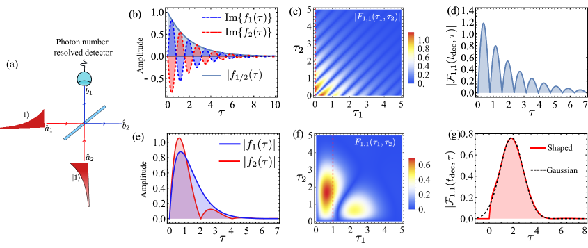
Figure 3: The temporal shaping scheme and examples. (a) Schematic for single photon temporal shaping based on the interference of two photon wavepackets and time resolved measurement. A photon number resolved detector is placed at the output port 1 of BS. (b)-(d) Single photon with ED sine shape generated via the interference of two ED shaped photons. (e)-(g) Single photon with Gaussian shape generated via the interference of two ED sine shaped photons. The detailed parameters are in the main text. (b), (e) The temporal shapes of the two input photons. (c), (f) The temporal shapes of the outcome $|1,1\rangle$. The red dashed line denotes the required detection time instant. (d), (g) The temporal shape of heralded single photon in output port 2 after time resolved detection.

We first note that theoretically, all three possible outcomes can be used for temporal shaping. However, only the wavefunction of component $|1,1\rangle$ can be controlled by adjusting the transmission of the BS, providing more degrees of freedom. Therefore, in this research, we primarily choose the component $|1,1\rangle$ to demonstrate measurement-based temporal shaping. The temporal shaping scheme is depicted in Fig. 3(a). Two photon wavepackets with different temporal shapes impinge on the BS and a photon number resolved photon detector is placed at the output port 1 of BS. By detecting only one photon at a specific time instant $t_{\text{dec}}$, the component $|1,1\rangle$ can be selected probabilistically. The resulting single photon state in output port 2 can be expressed as

$$\hat{b}_{1}(t_{\text{dec}})|1,1\rangle=\int F_{1,1}(t_{\text{dec}},\tau)\hat{b}_{2}^{\dagger}(\tau)d\tau|0,0\rangle$$ (9)

$$\underrightarrow{\text{norm}}|\Psi_{\text{dec}}\rangle=\frac{1}{\sqrt{\text{nor}}}\int F_{1,1}(t_{\text{dec}},\tau)\hat{b}_{2}^{\dagger}(\tau)d\tau|0,0\rangle$$

$$\equiv\int\mathcal{F}_{1,1}(t_{\text{dec}},\tau)\hat{b}_{2}^{\dagger}(\tau)d\tau|0,0\rangle,$$

with $\mathcal{F}_{1,1}(t_{\text{dec}},\tau)$ denotes the resulting temporal shape after detection

$$\mathcal{F}_{1,1}(t_{\text{dec}},\tau)=\frac{1}{\sqrt{\text{nor}}}\left(t^{2}f_{1}(t_{\text{dec}})f_{2}(\tau)-r^{2}f_{2}(t_{\text{dec}})f_{1}(\tau)\right).$$ (10)

Here ”norm” denotes the re-normalization of the state after detection. The normalization coefficient, $\text{nor}=\int|F_{1,1}(t,\tau)|^{2}d\tau$, ensures the proper normalization of the state. The shape of the heralded single photon $\mathcal{F}_{1,1}(t_{\text{dec}},\tau)$ in output port 2 depends on the temporal shapes of two input photons, the transmission of BS, and the time resolved measurement outcome at a time instant $t_{\text{dec}}$. The joint control of these parameters tailors the temporal shape.

IV.2 Example: Shaping photon from ED shape into ED sine shape

Photons generated by different types of single-photon sources exhibit variations in their temporal shapes, which can include ED shapes [30], ED sine shapes [31], and Gaussian shapes, etc. The temporal shape mismatch problem is common, which affects the interference of photons and the light-matter interactions, further affecting its application in the corresponding quantum information process. Here, we demonstrate that temporal shape mismatch can potentially be addressed through the measurement-based single-photon temporal shaping scheme.

We first show that the photon with ED sine shapes can be generated via the interference of two detuned ED-shaped photons through a symmetric 50/50 BS. The temporal shapes of the two input photons can be expressed as $f_{1/2}(\tau)=\sqrt{\Gamma}e^{-i(\pm\Delta\omega-i\Gamma)\tau/2}$, here $\Gamma,\Delta\omega$ denote the spectral width and detuning of two input photons, respectively. Following Eq. (4), the wavefucntion of the component $|1,1\rangle$ after passing the symmetric BS is

$$F_{1,1}(\tau_{1},\tau_{2})=i\sqrt{\frac{1}{P_{1,1}}}e^{-\Gamma(\tau_{1}+\tau_{2})/2}\sin(\Delta\omega(\tau_{2}-\tau_{1})/2).$$ (11)

By detecting only one photon at time instant $t_{\text{dec}}=0$ at output port 1 of BS, the temporal shape of the resulting single photon at port 2 is

$$\mathcal{F}_{1,1}(0,\tau)=i\sqrt{\frac{\Gamma\left(\Delta\omega^{2}+\Gamma^{2}\right)}{\Delta\omega^{2}/2}}e^{-\Gamma\tau/2}\sin(\Delta\omega\tau/2),$$ (12)

which is the required ED sine shape. Fig. 3(b)-(d) show an exact example. The temporal shapes of two input wavepackets with ED shapes are shown in Fig. 3 (b). The linewidth of the two photons are the same $\Gamma=1$ and the detuning is set to be $\Delta\omega=8$. The wavefunction of the component $|1,1\rangle$ after passing through the BS is depicted in Fig. 3 (c), where quantum beat pattern can be observed. By detecting only one photon at time instant $t_{\text{dec}}=0$ (red dashed lines) at port 1 of BS, the resulting single photon with ED sine temporal shape at port 2 is shown in Fig. 3(d).

IV.3 Example: Shaping photon from ED sine shape into Gaussian shape

A single-photon wavepacket with a Gaussian profile plays a crucial role in achieving high-fidelity deterministic optical quantum storage [15] and optical quantum logic gates [16, 32]. The Gaussian shape is also optimal for experiments relying on single-photon interference [33]. Now we demonstrate that a single-photon wavepacket with a Gaussian profile can be obtained through the interference of two photons with ED sine shapes. The temporal shape of the ED sine shaped photons can be described as $f_{n}(\tau)=\sqrt{\frac{\Gamma_{n}\left(4\omega_{n}^{2}+\Gamma_{n}^{2}\right)}{2\omega_{n}^{2}}}e^{-\Gamma_{n}t/2}\sin\left(\omega_{n}t\right)$, where $\Gamma_{n}$ and $\omega_{n}$ represent the spectral width and resonant frequency, respectively. The Gaussian shape can be expressed as $f_{\text{Gau}}(\tau)=\sqrt{\frac{\Gamma_{\text{Gau}}}{\sqrt{\pi}}}e^{-\frac{1}{2}(\tau-\tau_{0})^{2}\Gamma_{\text{Gau}}^{2}}$, where $\Gamma_{\text{Gau}}$ and $\tau_{0}$ denote the spectral width and the delay time of photon wavepacket, respectively. We aim for excellent indistinguishability between the interferometrically synthesized wavepacket and the Gaussian shape wavepacket. This translates into realizing the following optimization problem:

$$\text{Maximize: }F_{\text{shaping}}(x)=\left|\int f_{\text{Gau}}^{*}(\tau)\mathcal{F}_{1,1}(t_{\text{dec}},\tau)d\tau\right|^{2},$$ (13)

here $F_{\text{shaping}}$ represents the shaping fidelity, defined as the square of the indistinguishability between the interferometrically synthesized wavepacket and the Gaussian wavepacket. In optimization, the linewidth of the Gaussian shape $\Gamma_{\text{Gau}}$ is fixed to be 1, and the parameters to be optimized are $x=\left\{\Gamma_{1},\Gamma_{2},\omega_{1},\omega_{2},t,\tau_{0},t_{\text{dec}}\right\}$, including the linewidth of the input photons $\Gamma_{n}$, resonant frequency $\omega_{n}$, transmission coefficients $t$ of BS, delay time of the shaped Gaussian shape $\tau_{0}$ and an appropriate detection time $t_{\text{dec}}$. After optimization, we found that an optimized shaping fidelity of 0.996 can be achieved and the optimized parameters are $x=\left\{2.04,2.60,-1.49,0.380,0.768,1.81,0.940\right\}$. Figure 3(e) shows the temporal shapes of the two input photons, both of which are ED sine shapes. The wavefunction of $|1,1\rangle$ after passing through the BS is shown in Fig. 3(f), we can see that the output wavefucntion is entangled temporally. By detecting only one photon at output port 1 of BS at time $t_{\text{dec}}=0.940$, as indicated by the dashed lines in Fig. 3(f), the resulting single photon temporal shape at output port 2 of BS is drawn in Fig. 3(g). The objective Gaussian shape is also shown in Fig. 3(g) as a reference. We can observe that the temporal shape synthesized through interference is very similar to the ideal Gaussian shape.

In the above two examples, we have assumed that detectors could precisely detect photons at specific moments. However, in actual detection processes, the resolution of detectors is always limited. The effect of limited resolved time on heralding probability and fidelity is simulated in Appendix C. The limited resolved time of detectors could increase the heralding probability but decrease the fidelity. A trade-off between requirements of heralding probability and fidelity should be considered in experiments.

V Summary

In summary, we have studied the interference of two photon wavepackets with different temporal shapes through BS. We have employed the Von Neumann entropy to quantitatively describe the entanglement of the output state and found analytically that the entanglement is directly determined by the temporal indistinguishability of photons and the splitting ratio of BS. Maximum entanglement for the outcome $|1,1\rangle$ can be achieved with a 50/50 BS configuration, while completely distinguishable input photons will maximize the entanglement of the outcome $|2,0\rangle$ and $|0,2\rangle$. We have further demonstrated that the temporal shaping of a single photon can be achieved probabilistically by detecting one of the entangled photons. Our work reveals the crucial roles of photon temporal indistinguishability and photon pathway indistinguishability in the generation of temporal entanglement. The proposed scheme of single-photon temporal shaping also offers a solution to the issues of shape mismatch in complex large-scale optical quantum networks.

Appendix A Schmidt decomposition of the output state

To perform the Schmidt decomposition of the output state, the temporal correlation function $K_{m}\left(\tau_{1},\tau_{2}\right),\tilde{K}_{m}\left(\tau_{1},\tau_{2}\right)$ of the wavefunction $F_{m,2-m}(\tau_{1},\tau_{2})$ should be first obtained [26]

$$K_{m}\left(\tau_{1},\tau_{2}\right)=\int F_{m,2-m}\left(\tau_{1},\tau\right)F_{2-m}^{*}\left(\tau_{2},\tau\right)d\tau,$$ (14a)

$$\tilde{K}_{m}\left(\tau_{1},\tau_{2}\right)=\int F_{m,2-m}\left(\tau,\tau_{1}\right)F_{2-m}^{*}\left(\tau,\tau_{2}\right)d\tau,$$ (14b)

then the Schmidt modes $\phi_{n}^{m}(\tau),\tilde{\phi}_{n}^{m}(\tau)$ and coefficients $|\lambda_{n}^{m}|^{2}$ are solutions of the following integral eigenvalue equations

$$\int K_{m}\left(\tau,\tau^{\prime}\right)\phi_{i}^{m}\left(\tau^{\prime}\right)d\tau^{\prime}=\left|\lambda_{i}^{m}\right|^{2}\phi_{i}^{m}(\tau),$$ (15a)

$$\int\tilde{K}_{m}\left(\tau,\tau^{\prime}\right)\tilde{\phi}_{i}^{m}\left)\tau^{\prime}\right)d\tau^{\prime}=\left|\lambda_{i}^{m}\right|^{2}\tilde{\phi}_{i}^{m}(\tau),$$ (15b)

which should be done numerically in general. To analytically perform the Schmidt decomposition, we first construct the new orthogonal basis vector $\bm{\xi}(\tau)=[\xi_{1}(\tau),\xi_{2}(\tau)]^{T}$ via the Gram–Schmidt process based on the temporal shapes $f_{n}(\tau)$ of input photons

$$\xi_{1}(\tau)=f_{1}(\tau),$$ (16a)

$$\xi_{2}(\tau)=\frac{f_{2}(\tau)-J^{*}f_{1}(\tau)}{\mathcal{J}}.$$ (16b)

This way, the output temporal shapes are the coherent superposition of these orthogonal basis vectors

$$F_{2,0}\left(\tau_{1},\tau_{2}\right)=\frac{1}{\sqrt{2P_{2,0}}}\left[\mathcal{J}\xi_{1}\left(\tau_{1}\right)\xi_{2}\left(\tau_{2}\right)+\mathcal{J}\xi_{2}\left(\tau_{1}\right)\xi_{1}\left(\tau_{2}\right)+2J^{*}\xi_{1}\left(\tau_{1}\right)\xi_{1}\left(\tau_{2}\right)\right],$$ (17a)

$$F_{0,2}\left(\tau_{1},\tau_{2}\right)=-\frac{1}{\sqrt{2P_{0,2}}}\left[\mathcal{J}\xi_{1}\left(\tau_{1}\right)\xi_{2}\left(\tau_{2}\right)+\mathcal{J}\xi_{2}\left(\tau_{1}\right)\xi_{1}\left(\tau_{2}\right)+2J^{*}\xi_{1}\left(\tau_{1}\right)\xi_{1}\left(\tau_{2}\right)\right],$$ (17b)

$$F_{1,1}\left(\tau_{1},\tau_{2}\right)=\frac{1}{\sqrt{P_{1,1}}}\left[\mathcal{J}T\xi_{1}\left(\tau_{1}\right)\xi_{2}\left(\tau_{2}\right)-\mathcal{J}R\xi_{2}\left(\tau_{1}\right)\xi_{1}\left(\tau_{2}\right)+\mathcal{P}J^{*}\xi_{1}\left(\tau_{1}\right)\xi_{1}\left(\tau_{2}\right)\right].$$ (17c)

By inserting the results in Eq. (17) into Eq. (14), the temporal correlation function can be analytically expressed as follows

$$K_{m}\left(\tau_{1},\tau_{2}\right)=\bm{\xi}^{\mathrm{T}}\left(\tau_{1}\right)\mathbf{M}^{m}\bm{\xi}^{*}\left(\tau_{2}\right),$$ (18)

$$\tilde{K}_{m}\left(\tau_{1},\tau_{2}\right)=\bm{\xi}^{\mathrm{T}}\left(\tau_{1}\right)\tilde{\mathbf{M}}^{m}\bm{\xi}^{*}\left(\tau_{2}\right),$$ (19)

where $\tilde{\mathbf{M}}^{m},\tilde{\mathbf{M}}^{m}$ are the corresponding coefficient matrix

$$\mathbf{M}^{1} =\frac{1}{\sqrt{P_{1,1}}}\left(\begin{array}[]{cc}\mathcal{P}^{2}\left(1-\mathcal{J}^{2}\right)+T^{2}\mathcal{J}^{2}&-R\mathcal{J}\mathcal{P}J^{*}\\ -R\mathcal{J}\mathcal{P}J&T^{2}\mathcal{J}^{2}\end{array}\right),$$ (20c)

$$\tilde{\mathbf{M}}^{1} =\frac{1}{\sqrt{P_{1,1}}}\left(\begin{array}[]{cc}\mathcal{P}^{2}\left(1-\mathcal{J}^{2}\right)+R^{2}\mathcal{J}^{2}&T\mathcal{J}\mathcal{P}J^{*}\\ T\mathcal{J}\mathcal{P}J&T^{2}\mathcal{J}^{2}\end{array}\right),$$ (20f)

$$\mathbf{M}^{2/0} =\tilde{\mathbf{M}}_{2/0}=\frac{1}{\sqrt{2\left(1+|J|^{2}\right)}}\left(\begin{array}[]{cc}4-3\mathcal{J}^{2}&2J^{*}\mathcal{J}\\ 2\mathrm{~{}J}\mathcal{J}&\mathcal{J}^{2}\end{array}\right),$$ (20i)

and $T=t^{2},R=r^{2}$ are the transmission and reflection ratios of BS. By performing eigendecomposition on the coefficient matrix $\mathbf{M}^{m},\tilde{\mathbf{M}}^{m}$, the correlation functions can be expressed in the standard form of a Schmidt decomposition

$$K_{m}\left(\tau_{1},\tau_{2}\right) =\bm{\xi}^{\mathrm{T}}\left(\tau_{1}\right)\mathbf{V}^{m}\left(\begin{array}[]{cc}|\lambda_{1}^{m}|^{2}&0\\ 0&|\lambda_{2}^{m}|^{2}\end{array}\right)(\mathbf{V}^{m})^{-1}\bm{\xi}^{*}\left(\tau_{2}\right)$$ (21)

$$=\bm{\phi}^{\mathrm{T}}\left(\tau_{1}\right)\left(\begin{array}[]{cc}|\lambda_{1}^{m}|^{2}&0\\ 0&|\lambda_{2}^{m}|^{2}\end{array}\right)\bm{\phi}^{*}\left(\tau_{2}\right),$$

$$\tilde{K}_{m}\left(\tau_{1},\tau_{2}\right) =\xi^{\mathrm{T}}\left(\tau_{1}\right)\tilde{\mathbf{V}}^{m}\left(\begin{array}[]{cc}|\lambda_{1}^{m}|^{2}&0\\ 0&|\lambda_{2}^{m}|^{2}\end{array}\right)(\tilde{\mathbf{V}}^{m})^{-1}\xi^{*}\left(\tau_{2}\right)$$ (22)

$$=\tilde{\bm{\phi}}^{\mathrm{T}}\left(\tau_{1}\right)\left(\begin{array}[]{cc}|\lambda_{1}^{m}|^{2}&0\\ 0&|\lambda_{2}^{m}|^{2}\end{array}\right)\tilde{\bm{\phi}}^{*}\left(\tau_{2}\right).$$

Here $\mathbf{V}^{m}=[V_{1}^{m},V_{2}^{m}],\tilde{\mathbf{V}}^{m}=[\tilde{V}_{1}^{m},\tilde{V}_{2}^{m}]$ are the matrix composed of the eigenvectors of matrix $\mathrm{M}^{m},\tilde{\mathrm{M}}^{m}$, respectively. The eigenvalues of matrices $\mathbf{M}^{m},\tilde{\mathbf{M}}^{m}$ are the corresponding Schmidt coefficients $|\lambda_{n}^{m}|^{2}$. The Schmidt modes can be constructed via the orthogonal basis vector $\bm{\xi}(\tau)$ and the eigenvectors of matrices $\tilde{\mathrm{M}}^{m},\tilde{\mathrm{M}}^{m}$ as follows

$$\left(\begin{array}[]{l}\phi_{1}^{m}(\tau)\\ \phi_{2}^{m}(\tau)\end{array}\right)=\left[\mathbf{V}^{m}\right]^{\mathrm{T}}\left(\begin{array}[]{l}\xi_{1}(\tau)\\ \xi_{2}(\tau)\end{array}\right),$$ (23e)

$$\left(\begin{array}[]{l}\tilde{\phi}_{1}^{m}(\tau)\\ \tilde{\phi}_{2}^{m}(\tau)\end{array}\right)=\left[\tilde{\mathbf{V}}^{m}\right]^{\mathrm{T}}\left(\begin{array}[]{l}\xi_{1}(\tau)\\ \xi_{2}(\tau)\end{array}\right).$$ (23j)

Appendix B Example of the Schmidt decomposition and numerical validation

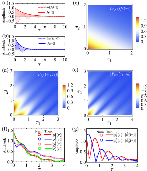
Figure 4: Example demonstrating the Schmidt decomposition of the output state and numerical validation of the analytical results. The temporal shape of two photon wavepackets input from (a) port 1 and (b) port 2 of BS. The absolute value of (c) the input two-photon wavefunction $|f_{1}(\tau_{1})f_{2}(\tau_{2})|$; The output two-photon wavefunction for the part (d) $|1,1\rangle$ and (e) $|2,0\rangle$; Comparison between the Schmidt modes from numerical simulations (circles) and from analytical results (solid curves) for the outcomes (f) $|1,1\rangle$ and (g) $|2,0\rangle$ . Here we take $\Gamma_{1}=1,\Gamma_{2}=2,\omega_{1}=-3,\omega_{2}=3$ and $t^{2}=1/4$.

As an exact example, we specifically consider the interference of two photons with different ED shapes $f_{n}(\tau)=\sqrt{\Gamma_{n}}e^{-i\left(\omega_{n}-\frac{\text{i$\Gamma$}_{n}}{2}\right)\tau}\Theta\left(\tau\right)$, where $\Theta$ is the Heaviside step function. $\Gamma_{n},\omega_{n}$ are the spectral width, and resonant frequency of photon wavepacket, respectively. Figure 4(a) and (b) show the temporal shapes of the two input photons, respectively. The absolute value is represented by solid curves, and the imaginary value is represented by dashed curves. The two-dimensional distribution of the two-photon wavefunction for the input quantum state is shown in Fig. 4 (c), which shows exponentially decay in both time axis $\tau_{1},\tau_{2}$. From Eq. (4), we know that the wavefunctions of the part $|2,0\rangle$ and $|0,2\rangle$ differ only by a sign. Therefore, in the following discussions on wavefunctions, we will primarily focus on the part $|2,0\rangle$. After passing through the BS, the output two-photon wavefunction $|F_{1,1}(\tau_{1},\tau_{2})|$ and $|F_{2,0}(\tau_{1},\tau_{2})|$ are shown in Fig. 4 (d), (e), respectively. We can observe that the temporally overlapping parts interfere either destructively or constructively, forming interference fringes. With time resolved detection, the interference fringes primarily manifest as the quantum beat effects of the second order correlation function [9]. The photon indistinguishability can be obtained by calculating the temporal overlap integral of the two input photons which is $|J|=0.229$. According to the analytical expression in Eq. (6), the Schmidt coefficients of the part $|2,0\rangle$ and $|1,1\rangle$ are $|\lambda^{2}_{1}|^{2}=0.283,|\lambda^{2}_{2}|^{2}=0.717,$ and $|\lambda^{1}_{1}|^{2}=0.905,|\lambda^{1}_{2}|^{2}=0.095$, respectively, confirming that the output states are entangled.

To verify the correctness of the analytical Schmidt decomposition results, we tackle the eigenvalue problem in Eq. (15) numerically. We discretize $K_{m}(\tau_{1},\tau_{2}),\tilde{K}_{m}(\tau_{1},\tau_{2})$ into a $100\times 100$ grid on a square temporal domain ranging from 0 to 10. The corresponding eigenvalues agree well with the analytical results. The Schmidt modes corresponding to outcomes $|1,1\rangle$ and $|2,0\rangle$ are depicted in Fig 4(f) and (g), respectively. We can observe that the temporal shape of Schmidt modes obtained from analytical expression (solid curves) and from numerical simulations (circles) exhibit good agreement.

Appendix C Schmidt decomposition of $|1,1\rangle$ for a 50/50 BS

Following the expression in Eq. (17), for a 50/50 BS, $t^{2}=r^{2}=1/2$, then $\mathcal{P}=0$, the wavefunction $F_{1,1}(\tau_{1},\tau_{2})$ turns out to be

$$F_{1,1}\left(\tau_{1},\tau_{2}\right)=\frac{1}{\sqrt{2}}\left[\xi_{1}\left(\tau_{1}\right)\xi_{2}\left(\tau_{2}\right)-\xi_{2}\left(\tau_{1}\right)\xi_{1}\left(\tau_{2}\right)\right],$$ (24)

which is already a standard form of the Schmidt decomposition, with the Schmidt modes as $\phi_{1}^{1}=\tilde{\phi}_{2}^{1}=\xi_{1}(\tau),\phi_{2}^{1}=\tilde{\phi}_{1}^{1}=\xi_{2}(\tau)$ and the Schmidt coefficients are $\lambda_{1/2}^{1}=\pm\frac{1}{\sqrt{2}}$.

Appendix D Effect of limited resolved time on heralding probability and fidelity

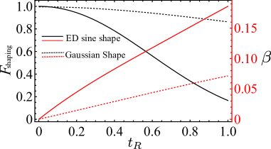
Figure 5: Effect of limited detection resolution $t_{R}$ on the fidelity (black lines) and heralding probability (red lines) for generating photon with ED shape (solid curves) and Gaussian shape (dashed curves).

The time interval that the detector could resolve is assumed to be $t_{R}$, the time resolved single photon detection process should be reformulated as follows:

$$\int_{t_{\text{dec}}-t_{R}/2}^{t_{\text{dec}}+t_{R}/2}\hat{b}_{1}(\tau)d\tau|1,1\rangle$$ (25)

$$=\int_{t_{\text{dec}}-t_{R}/2}^{t_{\text{dec}}+t_{R}/2}d\tau\int F_{1,1}(\tau_{1},\tau_{2})\hat{b}_{2}^{\dagger}(\tau_{2})d\tau_{2}|0,0\rangle$$

$$\underrightarrow{\text{norm}}|\Psi_{\text{dec}}\rangle=\int_{t_{\text{dec}}-t_{R}/2}^{t_{\text{dec}}+t_{R}/2}\int\frac{F_{1,1}(\tau_{1},\tau_{2})}{\sqrt{\text{nor}}}\hat{b}_{2}^{\dagger}(\tau_{2})d\tau_{2}|0,0\rangle.$$

Here the normalization coefficient becomes to be $\text{nor}=\int_{t_{\text{dec}}-t_{R}/2}^{t_{\text{dec}}+t_{R}/2}\int|F_{1,1}(\tau_{1},\tau_{2})|^{2}d\tau_{1}d\tau_{2}$. The heralding success probability, denoted as $\beta$, can be expressed as

$$\beta=P_{1,1}\left|\int_{t_{\text{dec}}-t_{R}/2}^{t_{\text{dec}}+t_{R}/2}d\tau_{1}\int d\tau_{2}|F_{m,2-m}(\tau_{1},\tau_{2})\right|^{2}.$$ (26)

Therefore, if the resolved time $t_{R}$ approaches to 0, the corresponding heralding probability approaches to 0 too. In the case of limited detection resolution, the fidelity could be re-expressed as

$$F_{\text{shaping}}=\left|\int_{t_{\text{dec}}-t_{R}/2}^{t_{\text{dec}}+t_{R}/2}d\tau_{1}\int d\tau_{2}\frac{F_{1,1}(\tau_{1},\tau_{2})}{\sqrt{\text{nor}}}\frac{f_{\text{Ideal}}^{*}(\tau_{2})}{\sqrt{t_{R}}}\right|^{2}.$$ (27)

The effect of limited resolved time $t_{R}$ on the heralding fidelity $F_{\text{shaping}}$ and success probability $\beta$ for ED shape and Gaussian shapes is shown in Fig. 5. We can observe that with the increase of the resolved time $t_{R}$, the heralding probability gradually increases from zero, while the fidelity decreases from its maximum value.

References

- Hong et al. [1987] C. K. Hong, Z. Y. Ou, and L. Mandel, Phys. Rev. Lett. 59, 2044 (1987).
- Knill et al. [2001] E. Knill, R. Laflamme, and G. J. Milburn, Nature 409, 46 (2001).
- Kok et al. [2007] P. Kok, W. J. Munro, K. Nemoto, T. C. Ralph, J. P. Dowling, and G. J. Milburn, Rev. Mod. Phys. 79, 135 (2007).
- Vittorini et al. [2014] G. Vittorini, D. Hucul, I. V. Inlek, C. Crocker, and C. Monroe, Phys. Rev. A 90, 040302 (2014).
- Laibacher and Tamma [2018] S. Laibacher and V. Tamma, Phys. Rev. A 98, 053829 (2018).
- Zhao et al. [2014] T.-M. Zhao, H. Zhang, J. Yang, Z.-R. Sang, X. Jiang, X.-H. Bao, and J.-W. Pan, Phys. Rev. Lett. 112, 103602 (2014).
- Legero et al. [2003] T. Legero, T. Wilk, A. Kuhn, and G. Rempe, Applied Physics B 77, 797 (2003).
- Tamma and Laibacher [2015] V. Tamma and S. Laibacher, Phys. Rev. Lett. 114, 243601 (2015).
- Legero et al. [2004] T. Legero, T. Wilk, M. Hennrich, G. Rempe, and A. Kuhn, Phys. Rev. Lett. 93, 070503 (2004).
- Wang et al. [2018] X.-J. Wang, B. Jing, P.-F. Sun, C.-W. Yang, Y. Yu, V. Tamma, X.-H. Bao, and J.-W. Pan, Phys. Rev. Lett. 121, 080501 (2018).
- Rephaeli et al. [2010] E. Rephaeli, J.-T. Shen, and S. Fan, Phys. Rev. A 82, 033804 (2010).
- Rephaeli and Fan [2012] E. Rephaeli and S. Fan, Phys. Rev. Lett. 108, 143602 (2012), publisher: American Physical Society.
- Calajó et al. [2019] G. Calajó, Y.-L. L. Fang, H. U. Baranger, and F. Ciccarello, Phys. Rev. Lett. 122, 073601 (2019).
- Cotrufo and Alù [2019] M. Cotrufo and A. Alù, Optica 6, 799 (2019).
- Cirac et al. [1997] J. I. Cirac, P. Zoller, H. J. Kimble, and H. Mabuchi, Phys. Rev. Lett. 78, 3221 (1997).
- Heuck et al. [2020] M. Heuck, K. Jacobs, and D. R. Englund, Phys. Rev. Lett. 124, 160501 (2020).
- Tian et al. [2021] Z. Tian, P. Zhang, and X.-W. Chen, Phys. Rev. Appl. 15, 054043 (2021).
- Yanik and Fan [2004] M. F. Yanik and S. Fan, Phys. Rev. Lett. 93, 173903 (2004).
- Yuan et al. [2016] L. Yuan, M. Xiao, and S. Fan, Phys. Rev. B 94, 140303(R) (2016).
- Baek et al. [2008] S.-Y. Baek, O. Kwon, and Y.-H. Kim, Phys. Rev. A 77, 013829 (2008).
- Averchenko et al. [2017] V. Averchenko, D. Sych, G. Schunk, U. Vogl, C. Marquardt, and G. Leuchs, Phys. Rev. A 96, 043822 (2017).
- Sych et al. [2017] D. Sych, V. Averchenko, and G. Leuchs, Phys. Rev. A 96, 053847 (2017).
- Blow et al. [1990] K. J. Blow, R. Loudon, S. J. D. Phoenix, and T. J. Shepherd, Phys. Rev. A 42, 4102 (1990).
- Orre et al. [2019] V. V. Orre, E. A. Goldschmidt, A. Deshpande, A. V. Gorshkov, V. Tamma, M. Hafezi, and S. Mittal, Phys. Rev. Lett. 123, 123603 (2019).
- Gerrits et al. [2015] T. Gerrits, F. Marsili, V. B. Verma, L. K. Shalm, M. Shaw, R. P. Mirin, and S. W. Nam, Phys. Rev. A 91, 013830 (2015).
- Law et al. [2000] C. K. Law, I. A. Walmsley, and J. H. Eberly, Phys. Rev. Lett. 84, 5304 (2000).
- Pe’er et al. [2005] A. Pe’er, B. Dayan, A. A. Friesem, and Y. Silberberg, Phys. Rev. Lett. 94, 073601 (2005).
- Srivathsan et al. [2014] B. Srivathsan, G. K. Gulati, A. Cerè, B. Chng, and C. Kurtsiefer, Phys. Rev. Lett. 113, 163601 (2014).
- Liu et al. [2014] C. Liu, Y. Sun, L. Zhao, S. Zhang, M. M. T. Loy, and S. Du, Phys. Rev. Lett. 113, 133601 (2014).
- Arcari et al. [2014] M. Arcari, I. Söllner, A. Javadi, S. Lindskov Hansen, S. Mahmoodian, J. Liu, H. Thyrrestrup, E. H. Lee, J. D. Song, S. Stobbe, and P. Lodahl, Phys. Rev. Lett. 113, 093603 (2014).
- Johne and Fiore [2011] R. Johne and A. Fiore, Phys. Rev. A 84, 053850 (2011).
- Li et al. [2020] M. Li, Y.-L. Zhang, H. X. Tang, C.-H. Dong, G.-C. Guo, and C.-L. Zou, Phys. Rev. Appl. 13, 044013 (2020).
- Rohde et al. [2005] P. P. Rohde, T. C. Ralph, and M. A. Nielsen, Phys. Rev. A 72, 052332 (2005).