Medium Assisted Low Energy Nuclear Fusion

Abstract

We study the process of nuclear fusion at low energies in a medium using the second order time dependent perturbation theory. We consider a specific process which involves fusion of a low energy proton with a Nickel nucleus. The reaction proceeds in two steps or interactions. We refer to the amplitudes corresponding to these two interactions as the molecular and the nuclear matrix elements. The first amplitude involves Coulomb interaction with another nucleus in the medium while the second corresponds to the nuclear fusion process. Due to the presence of high energy intermediate states, the repulsive Coulomb barrier may be evaded at this order. However, it has been shown in earlier papers that contributions from different intermediate states cancel one another leading to negligible amplitude unless it is assisted by special medium effects. The medium leads to localization of eigenstates and resultant discretization of energy eigenvalues which evades the acute cancellation and leads to observable rate. In the present paper we extend this mechanism to consider the fusion of a light nucleus with a heavy nucleus. To be specific we consider the fusion of proton with Nickel to form Copper with emission of a photon. The process is assisted by the presence of an impurity ion in the medium.

1 Introduction

There exists considerable experimental evidence for nuclear fusion reactions at low energies [1, 2, 3, 4, 5, 6, 7, 8, 9, 10]. Theoretically, there have been many attempts to explain these processes in terms of electron screening [11, 12, 13], correlated states [14, 15], electroweak interactions [16], formation of clusters of nuclear particles [17], relativistic electrons in deep orbits [18] and phonon induced reactions [19]. A critical review of many claims in this field is provided in [20].

In the present paper we study the possibility that such reactions may proceed at second order in time dependent perturbation theory [21, 22, 23, 24, 25]. The first perturbation causes the system to go into a state which is a linear superposition of all eigenstates of the unperturbed Hamiltonian. Due to the presence of eigenstates of relatively high energy, it is possible that the Coulomb barrier may not be a very serious issue. Although the amplitude for such high energy eigenstates is suppressed, the suppression may not be as strong as that due to the Coulomb barrier. We applied this formalism explicitly to the process involving fusion of proton with deuteron to form helium nucleus with $A=3$ [22, 23]. The perturbation was assumed to be electromagnetic leading to either emission or absorption of photons. The dominant process was found to be the one in which two photons are spontaneously emitted. We need to sum over all intermediate states up to infinite energy. We assume that the momentum of the photon emitted at the first (molecular) vertex is relatively large. The amplitude for the process is found to substantial for some fixed values of intermediate energies, if the relative proton-deuteron momentum is approximately opposite to the momentum of the photon emitted at the first vertex. Here we assume that this momentum is sufficiently large that the Coulomb barrier does not lead to a strong suppression. Although the amplitude is significant for some range of energies, we find that as we sum over all intermediate states, the amplitude adds up to very small values if we assume free space boundary conditions at large distances. Hence, the rate is found to be very small in free space. We obtain contributions from large number of intermediate states since the eigenstates of the unperturbed Hamiltonian are not momentum eigenstates. In particular, due to the Coulomb repulsion, the initial state deviates considerably from being a momentum eigenstate.

Although the rate is found to be highly suppressed in free space, it was argued that in a medium, under special conditions, the rate may be significant and observable [22, 23]. This was explicitly shown to work in a simple model [24]. The basic idea in this paper is that in a medium the boundary conditions on the wave function at large distance gets modified, leading to discretization of energy eigenvalues. Furthermore, in the presence of disorder, the eigenfunctions get localized [26, 27]. We point out that phenomenon being discussed here is different from Anderson localization [26, 27] since we considering the medium wave function of a proton (or other nuclei) and not electron. Furthermore, we are dominantly interested in states with energy eigenvalues less than the medium potential height. If we assume such localized states, we do not find the acute cancellation of amplitudes that was found in free space. In [24] we used a simple step potential to model the tunneling barrier but the mechanism is expected to work also for Coulomb barrier. The model can directly be applied to fusion of light nuclei within a medium composed of heavy nuclei. The energy of intermediate states required in this case is of the order of few tens of keV. For such energies, it is concievable that the wave functions would be localized in a medium.

In the present paper we apply this mechanism to the fusion of proton ¹H and a heavy nucleus ^AX of atomic number $Z$ and atomic mass $A$. This requires much higher intermediate state energies in comparison to fusion of two light nuclei and we consider a generalization of the mechanism used in [24]. At the first vertex, the process is assisted by an additional particle which we assume to be a heavy nucleus Y with atomic mass $A_{Y}$ [21]. Here, we assume $Y$ to be another Nickel nuclei present in the medium. At the second vertex proton undergoes fusion with the nucleus $X$ with emission of a photon. The basic process can be written as,

$$p+{}^{A}{\rm X}+{\rm Y}\rightarrow{}^{A+1}{\rm X^{\prime}}+{\rm Y}(\vec{k}_{Y})+\gamma(\vec{k}_{\gamma})$$ (1)

where the initial state particles have negligible momentum and the final state momenta are indicated in this equation. The process is illustrated in Fig. 1. Here we are showing only the nuclear states. In the initial state the proton and the X nucleus is assumed to form a molecular bound state, which is not explicitly indicated in the above equation. The Y atom is present in the vicinity and its nucleus interacts with the molecule through screened Coulomb interaction. This interaction leads to exchange of energy between Y and the molecule and produces a free Y particle of relatively high momentum [21]. This also breaks up the molecule, producing two particles with high relative momentum. A part of the momentum is transfered to the overall center of mass motion. Due to the high relative momentum, the two particles can now undergo nuclear fusion. However we need to coherently add contributions from all intermediate states that contribute.

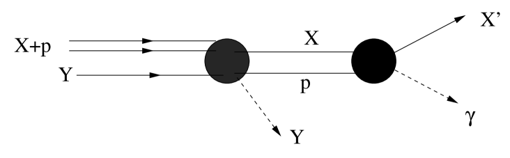
Figure 1: Schematic illustration of the reaction described in Eq. 1.

In earlier papers [22, 23, 24], we had considered emission of a photon at the first vertex. The main advantage of exchanging momentum with a heavy nucleus Y instead of a photon is that the nuclear particles can acquire much higher momenta in the latter case. Hence, although momentum required for fusion between two light nuclei at appreciable rates can be acquired by emission of a photon, this is not possible in the present case of fusion between a proton and a heavy nucleus. This process, however, suffers from the same problems as those with emission of a photon, that is, while the amplitude for the process becomes high for some intermediate states, overall the amplitude tends to cancel as we sum over all states [22, 23, 24]. The main point of this paper is the presence of special conditions which avoid this cancellation.

2 Proton-X fusion at second order in perturbation theory

Let us denote the position vectors of the proton and X by $\vec{r}_{1}$ and $\vec{r}_{2}$. The position vector of the Y particle is denoted by $\vec{r}_{3}$. We denote the relative and the CM coordinates of the system of particles 1 and 2 as

$$\vec{r}_{12} = \vec{r}_{1}-\vec{r}_{2}$$

$$\vec{R}_{12} = {m_{1}\vec{r}_{1}+m_{2}\vec{r}_{2}\over m_{1}+m_{2}}$$ (2)

In the initial state we have a molecular bound state along with a free Y particle. We can express the wave function as,

$$\Psi_{i}(\vec{r}_{1},\vec{r}_{2},\vec{r}_{3})=\psi_{i}(\vec{r}_{1},\vec{r}_{2})\psi_{Yi}(\vec{r}_{3})$$ (3)

The Y particle is assumed to be free and we take its wave function to be a plane wave of almost negligible momentum. The remaining two particles form a bound state. We assume that the overall center of mass motion acts as a free particle. Hence the wave function can be expressed as,

$$\psi_{i}(\vec{r}_{1},\vec{r}_{2})=\psi_{12i}(\vec{R}_{12})\chi_{12i}(\vec{r}_{12})$$ (4)

where the center of mass wave function $\psi_{12i}$ takes the form of a plane wave. We assume its momentum to be almost zero.

After Coulomb interaction with the Y particle the molecule breaks up leading to a large relative momentum between the two particles. The center of mass of the proton-X again behaves as a free particle. The relative coordinate $\vec{r}_{12}$ dependence of the wave function of this system is more complicated since the two particles undergo strong Coulomb repulsion along with the nuclear force at very short distances. The intermediate state wave function can be expressed as,

$$\Psi_{n}(\vec{r}_{1},\vec{r}_{2},\vec{r}_{3})=\psi_{12n}(\vec{R}_{12})\chi_{12n}(\vec{r}_{12})\psi_{Yn}(\vec{r}_{3})$$ (5)

Here the center of mass wave function $\psi_{12n}$ and the $Y$ particle wave function $\psi_{Yn}$ are taken to be plane waves. The wave function $\chi_{12n}$, which depends on the relative coordinate, is discussed below.

The Hamiltonian of the system is given by

$$H=H_{0}+H_{I}$$ (6)

where $H_{0}$ denote the unperturbed Hamiltonian and $H_{I}$ is the perturbation. The unperturbed part contains the kinetic energy terms and screened Coulomb and nuclear potentials corresponding to the proton-X system. Hence we can express $H_{0}$ as

$$H_{0}=K_{p}+K_{X}+K_{Y}+V_{12}(\vec{r}_{12})$$ (7)

where $K_{p}$, $K_{X}$ and $K_{Y}$ represent the kinetic energies of the proton, X and the Y particles respectively and $V_{12}$ is the potential between the proton and the X nucleus. Here $V_{12}$ contains the screened Coulomb potential along with the nuclear potential. As discussed later, these two particles may also experience the effect of medium at large distance which is also part of this potential. We assume a shell model nuclear potential, given by,

$$V_{nuc}=-{V_{0}\over 1+\exp((r-r_{nuc})/r_{0})}$$ (8)

where the parameter $r_{nuc}=1.25A^{1/3}$ fm, $r_{0}=0.524$ fm and $V_{0}=36$ MeV. The value of $V_{0}$ is chosen to obtain the expected energy eigenvalue of the nuclear bound state for nucleus under consideration. Hence the potential takes the form [28],

$$V = V_{nuc}\ \ \ \ \ \ \ \ \ \ \ \ \ \ \ \ \ \ \ \ \ \ r\leq r_{cut}$$ (9)

$$= {Z_{p}Z_{X}\over r}\ \ \ \ \ \ \ \ \ \ \ \ \ \ \ \ \ \ \ \ r>r_{cut}$$

where $Z_{p}$ and $Z_{X}$ are the atomic numbers of the proton and the X nuclei respectively and $r_{cut}$ is given by [28],

$$r_{cut}=1.4(A_{p}^{1/3}+A_{X}^{1/3})\times 10^{-13}\ \ {\rm cm}$$ (10)

Here $A_{p}$ and $A_{X}$ are the atomic mass numbers of the two particles and we have only displayed the bare Coulomb potential and not the screening part.

The interaction Hamiltonian can be split into two parts,

$$H_{I}=H_{I1}+H_{I2}$$ (11)

where $H_{I1}$ contains the Coulomb interaction between proton and Y and X and Y while $H_{I2}$ is given by [29, 30],

$$H_{I2}(t)=\sum_{i}{Z_{i}e\over cm_{i}}\vec{A}(\vec{r}_{i},t)\cdot\vec{p}_{i}$$ (12)

Here $Z_{i}$, $m_{i}$, $\vec{r}_{i}$ and $\vec{p}_{i}$ are respectively the charge, mass, position vector and momentum vector of the particle $i$. The electromagnetic field operator $\vec{A}(\vec{r},t)$ is given by

$$\vec{A}(\vec{r},t)={1\over\sqrt{V}}\sum_{\vec{k}}\sum_{\beta}c\sqrt{\hbar\over 2\omega}\left[a_{\vec{k},\beta}(t)\vec{\epsilon}_{\beta}e^{i\vec{k}\cdot\vec{r}}+a^{\dagger}_{\vec{k},\beta}(t)\vec{\epsilon}^{\,*}_{\beta}e^{-i\vec{k}\cdot\vec{r}}\right]$$ (13)

We point out that the Coulomb interaction between proton and X must be considered as part of the unperturbed Hamiltonian. This is because we are interested in fusion between these two particles and the full potential including contributions from Coulomb repulsion and nuclear attraction must be included in the unperturbed wave functions.

The leading order contribution to the process in Eq. 1 is obtained at second order in the time dependent perturbation theory. Let the wave vectors of the emitted photon be $\vec{k}_{\gamma}$ and the frequency be $\omega$. The transition amplitude at this order can be expressed as,

$$\langle f|T(t_{0},t)|i\rangle=\left(-{i\over\hbar}\right)^{2}\sum_{n}\int_{t_{0}}^{t}dt^{\prime}e^{i(E_{f}-E_{n})t^{\prime}/\hbar}\langle f|H_{I}(t^{\prime})|n\rangle\int_{t_{0}}^{t^{\prime}}dt^{\prime\prime}e^{i(E_{n}-E_{i})t^{\prime\prime}/\hbar}\langle n|H_{I}(t^{\prime\prime})|i\rangle\ .$$ (14)

where the sum is over the intermediate proton-X states. At the first vertex, the Y particle interacts with the proton and the X nucleus through the screened Coulomb potential, i.e. the interaction Hamiltonian $H_{I1}$ [21]. We refer to the corresponding amplitude as the molecular matrix element. At the second vertex the proton and X undergo nuclear fusion while emitting a photon through the interaction Hamiltonian $H_{I2}$. The corresponding amplitude is called the nuclear matrix element.

2.1 Molecular Matrix Element

Let us first consider the transition from initial to intermediate state through the Coulomb interaction. The matrix element can be written as

$$\langle n|H_{I1}|i\rangle=\int d^{3}r_{1}d^{3}r_{2}d^{3}r_{3}\Psi_{n}^{*}\left[V_{s}(p,Y)+V_{s}(X,Y)\right]\Psi_{i}$$ (15)

where $V_{s}(a,b)$ is the screened Coulomb potential [21],

$$V_{s}(a,b)={Z_{a}Z_{b}e^{2}\over 2\pi^{2}}\int d^{3}q{e^{i\vec{q}\cdot(\vec{r}_{a}-\vec{r}_{b})}\over q^{2}+q^{2}_{s}}$$ (16)

Here $q_{s}$ is the contribution due to screening. As we will see the contribution from the second term in Eq. 15 will be relatively small and we focus on the first term. We change variables to $\vec{r}_{12}$, $\vec{R}_{12}$ and $\vec{r}_{3}$ and set $\psi_{Yn}=e^{i\vec{k}_{3}\cdot\vec{r}_{r}}/\sqrt{V}$ and $\psi_{Yi}\approx 1/\sqrt{V}$. Here we have assumed negligible momentum for Y in the initial state. After integrating over $\vec{r}_{3}$ we obtain,

$$\langle n|H_{I1}|i\rangle={4\pi Z_{p}Z_{Y}e^{2}\over V}\int d^{3}r_{12}d^{3}R_{12}d^{3}q\psi_{12n}^{*}\chi_{12n}^{*}e^{i\vec{q}\cdot r_{1}}{\delta^{3}(\vec{k}_{3}+\vec{q})\over q^{2}+q_{s}^{2}}\psi_{12i}\chi_{12i}+...$$ (17)

Integrating over $\vec{q}$ we obtain

$$\langle n|H_{I1}|i\rangle={4\pi Z_{p}Z_{Y}e^{2}\over V}\int d^{3}r_{12}d^{3}R_{12}\psi_{12n}^{*}\chi_{12n}^{*}e^{-i\vec{k}_{3}\cdot\vec{r}_{1}}{1\over k_{3}^{2}}\psi_{12i}\chi_{12i}+...$$ (18)

Here we have dropped $q^{2}_{s}$ since we shall set $k^{2}_{3}>>q^{2}_{s}$. We next replace $\vec{r}_{1}=\vec{R}_{12}+\vec{r}_{12}m_{2}/(m_{1}+m_{2})$ and take the initial and intermediate center of mass wave functions to be plane waves. The intermediate center of mass momentum is taken to be $\vec{K}_{12}$ while the initial momentum is assumed to be negligible. Integration over $d^{3}R_{12}$ leads to a delta function $\delta^{3}(\vec{K}_{12}+\vec{k}_{3})$ and we focus on the integral in terms of relative variables. We obtain

$$\langle n|H_{I1}|i\rangle={4\pi Z_{p}Z_{Y}e^{2}\over Vk_{3}^{2}}I_{i}+...$$ (19)

where

$$I_{i}=\int d^{3}r_{12}\chi_{12n}^{*}e^{-i\vec{k}_{3}\cdot\vec{r}_{12}m_{2}/(m_{1}+m_{2})}\chi_{12i}$$ (20)

In the exponent the ratio of masses is approximately unity with $m_{2}>>m_{1}$ ($m_{X}>>m_{p}$). We will assume that the magnitude of $k_{3}$ is very large.

We next discuss the wave function $\chi_{12i}$ and $\chi_{12n}$ which depend on the relative coordinate $\vec{r}_{12}$. At short distance both of these are determined by the spherically symmetry nuclear potential along with the Coulomb repulsion. However their large distance behaviour is determined by the medium effects. The important point of this paper is that this large distance behaviour has very significant effect on the nuclear reaction. Hence by suitably choosing or tuning the medium we can change the nuclear reaction rate by orders of magnitude. We point out that in free space, assuming spherical symmetry, the reaction rate is negligible.

The initial state wave function $\chi_{12i}$ is an eigenstate of the unperturbed Hamiltonian $H_{0}$, corresponding to a very low energy eigenvalue. We assume this to be bound state wave function. The proton experiences the spherically symmetric repulsive Coulomb potential of the nucleus $X$ at short distances and hence the wave function decays very strongly at distances $r_{12}<1$. At intermediate distances, i.e. distances scales of a few Bohr radius, it experiences the attractive molecular potential. At larger distances it experiences the repulsive potential due to all the other ions present in the medium. The medium potential is likely to be complicated and is not expected to show any simple symmetry, especially in the presence of disorder. Here we do not attempt a detailed computation of the wave function and make simple assumptions about its nature. We assume that the wave function has roughly the same behaviour in all directions and hence can be approximated to be a function of only the radial distance $r_{12}$. Furthermore, we assume the potential to be approximately constant over the range $\Delta\leq r_{12}\leq r_{u}$ and strongly repulsive outside this range. The wave function can, therefore, be expressed as

$$\chi_{12i}=NY_{0}^{0}{\sin[(r_{12}-\Delta)/r_{0}]\over r_{12}}$$ (21)

for $\Delta\leq r_{12}\leq\pi r_{0}+\Delta$ and zero outside this range. The wave function can be smoothed at the two ends, as applicable for a finite potential barrier. However, this does not affect our results significantly. Here $N$ is the normalization, the parameter $\Delta$ is taken to be about 1 atomic unit and $r_{0}$ is of the order of the typical molecular distances.

In order to compute the total amplitude we need to sum over all the intermediate state wave functions $\chi_{12n}$ that can contribute. These are also eigenstates of the unperturbed Hamiltonian $H_{0}$. The dominant contribution is obtained from eigenstates of relatively large energy eigenvalue. At small distance these are solutions to the spherically symmetric nuclear potential including the Coulomb barrier. At large distances their behaviour is also determined by the molecular potential and the medium properties. Due to their high energy, these states may extend over the entire medium and, hence, the large scale structure of the medium has to be considered, which does not display spherical symmetry. For example, in a periodic crystalline lattice, all eigenstates are of the form of Bloch functions, $\psi(\vec{r})=u(\vec{r})e^{i\vec{k}\cdot\vec{r}}$ where the function $u(\vec{r})$ also displays the periodicity of the lattice. Here we do not go into a detailed solution of the Schrodinger equation in a medium and make some physically motivated assumptions. We assume that the medium is not periodic and displays disorder. In such a case, the eigenfunctions up to some maximum energy eigenvalue must be localized [26, 27]. Here we are interested in eigenstates with very high energy, but whose wave vectors $\vec{k}_{12}$ are large only in one direction, i.e. $\vec{k}_{12}\approx-\vec{k}_{3}$. We choose the z-axis along $\vec{k}_{3}$. The $z$ dependence of the wave function can be approximated as $e^{ik_{z}z}$. This is not significantly affected by the medium, which may lead to a slow modulation of the plane wave behaviour which is being ignored here. Due to the large value of $|k_{z}|$ we assume that it takes almost continuous range of values. However, in the transverse direction the behaviour of the wave function is determined by the transverse wave numbers $|k_{x}|$ and $|k_{y}|$ which are very small compared to $|k_{z}|$. Hence it is reasonable to assume that in these directions the wave function may be significantly modulated by the behaviour of the medium potential, leading to localization of wave function in these directions and discretization of $k_{x}$ and $k_{y}$. For simplicity, we assume that the wave function displays approximate cylindrical symmetry and is a function only of $\rho=r\sin\theta$. We denote it by $f(\rho)$ and write the full wave function as,

$$\chi_{12n}(\vec{r}_{12})={1\over\sqrt{L}}e^{ik_{z}z}f(\rho)$$ (22)

where $k_{12}^{2}=k_{z}^{2}+k_{\rho}^{2}$ and $k_{\rho}<<|k_{z}|$. Excluding very small values of $\rho$, comparable to nuclear distances, the wavefunction $f(\rho)\approx N_{n}(k_{\rho})J_{0}(k_{\rho}\rho)$, where $J_{0}$ is the Bessel function and $N_{n}$ is the normalization factor.

As discussed above, the function $f(\rho)$ is localized in space. We assume that it is zero for $\rho>\rho_{0}$. For simplicity, we take the upper length scale $\rho_{0}$ to be equal to $r_{u}=\pi r_{0}+\Delta$ which is same as that in the case of $\chi_{12i}$. Such a boundary condition is applicable for an infinite potential. For the case of a finite potential, we expect a smooth transition. However, this is not expected to significantly affect our results. Furthermore, by explicit calculations, we find that the amplitude decreases relatively slowly as we increase the value of $\rho_{0}$ and, hence, the chosen value gives a reasonable description of the physical process under consideration.

At small distances, of order nuclear scale, we need to match this solution to the nuclear tunneling wave function. This is obtained by solving the Schrodinger equation in the spherically symmetric nuclear potential including the Coulomb repulsion. The dominant contribution is obtained from the $l=0$ wave function, which depends on $k=\sqrt{k_{z}^{2}+k_{\rho}^{2}}$. For the values of $E_{n}$ of interest, with $|k_{z}|>>k_{\rho}$, it only shows a very mild dependence on $k_{\rho}$. Hence the nuclear matrix element cannot depend significantly on the value of $k_{\rho}$ which is much smaller than $k_{z}$. Therefore, it is reasonable to assume that the projection of $f(\rho)$ on the spherically symmetric $l=0$ short distance wave function is approximately constant, independent of $k_{\rho}$ for small $k_{\rho}$. We approximate the constant value of this wave function for small $\rho$ to be $N_{n}(k_{\rho 1})$, i.e. the normalization corresponding to the first zero of the Bessel function. We clarify that the actual value of the function $f(\rho)$ at very small $\rho$ may be somewhat different from the value assumed here, however, the essential point is that it cannot depend significantly on $k_{\rho}$.

The form of the wave function given in Eq. 22 follows by solving the Schrodinger equation using an approximation similar to the Born-Oppenheimer approximation. We note that wave function varies very rapidly along the z-direction and slowly along the transverse direction. Hence, we first solve the Schrodinger equation to determine the $z$ dependence for a fixed $\rho$. The solution obtained leads to an effective potential for the $\rho$ dependence and we can obtain the $\rho$ dependence by solving the resulting equation. This is illustrated in Appendix A. The essential assumption in obtaining Eq. 22 is that the $z$ dependence can be taken to be a plane wave to a good approximation. This is reasonable since the corresponding wave number $k_{z}$ is very large. However, as we shall see later, dominant contribution is obtained from small values of the transverse wave number $k_{\rho}$. Hence, the corresponding wave function may be strongly affected by the medium potential and is expected to decay rapidly at large $\rho$ leading to localization in the transverse plane and discretized values of $k_{\rho}$.

As mentioned above, we also need to match the large and short distance wave functions. The function $f(\rho)$ goes to a constant at small distance and we use the standard expansion for the plane wave,

$$e^{i\vec{k}\cdot\vec{r}}=4\pi\sum_{l=0}^{\infty}\sum_{m=-l}^{l}i^{l}j_{l}(kr)\ Y_{l}^{m}(\hat{r})Y_{l}^{m*}(\hat{k})$$ (23)

For energies under consideration the $l=0$ part will dominate and the high angular momentum contributions will be strongly suppressed due to Coulomb repulsion. We solve the Schrodinger equation for small $r_{12}$ in the presence of the nuclear and the Coulomb potential for $l=0$. The difference between this and the $l=0$ component of Eq. 23 is a scattered wave which will decay at large $r$ and hence can be neglected. The wave function may deviate from the assumed form at intermediate distances. However these play negligible role in the determination of the amplitude.

Before ending this section we explain why the contribution due the second term on the right hand side in Eq. 15 is relatively small. This is because the exponent in Eq. 19 in this case depends on the mass ratio $m_{1}/(m_{1}+m_{2})$ which is approximately $m_{p}/m_{X}<<1$. In contrast, in the first term the mass ratio is approximately unity and dominant contribution is obtained for $k_{12}$ of order $k_{3}$. Hence, the dominant contribution from second term will be obtained for $k_{12}$ much smaller than $k_{3}$ and will be suppressed.

2.2 Nuclear Matrix Element

We next consider the nuclear matrix element $\langle f|H_{I}(t^{\prime})|n\rangle$. In this case, the intermediate state proton undergoes fusion with the heavy nucleus with photon emission. The process is complicated since as the proton interacts with the nucleus, it can interact with all the nucleons, leading to a change in the multiparticle wave function. Here we assume that we can treat the nucleus $X$ as a single particle of charge $Z_{X}$. We denote the emitted photon momentum by $\vec{k}_{\gamma}$ and energy by $E_{\gamma}$. Let the angular coordinates of this photon momentum be $(\theta_{\gamma},\phi_{\gamma})$, i.e.,

$$\vec{k}_{\gamma}=k_{\gamma}\left[\cos\theta_{\gamma}\,\hat{z}+\sin\theta_{\gamma}(\cos\phi_{\gamma}\,\hat{x}+\sin\phi_{\gamma}\,\hat{y})\right]$$ (24)

The two polarization vectors of this photon can be expressed as

$$\vec{\epsilon}_{a} = -\sin\theta_{\gamma}\,\hat{z}+\cos\theta_{\gamma}(\cos\phi_{\gamma}\,\hat{x}+\sin\phi_{\gamma}\,\hat{y})$$

$$\vec{\epsilon}_{b} = -\sin\phi_{\gamma}\,\hat{x}+\cos\phi_{\gamma}\,\hat{y}$$ (25)

In order to proceed further we need to specify the final state eigenfunction. We take this state to be $l=1$, $j=3/2$ shell model state with one unpaired proton in the outer most shell. We shall consider the state for which proton has spin up and set $j_{z}=3/2$. We point out that ⁶²Ni (spin 0) satisfies our requirements. With addition of one more proton, this makes a transition to ⁶³Cu. Using the nuclear potential (Eq. 8), we find that the energy eigenvalue of this state is 9.1 MeV in good agreement with the observed value.

We perform the calculation by specializing to a particular polarization vector $\vec{\epsilon}_{b}$ of the emitted photon. Let $\vec{R}^{\prime}$ be the final state center of mass coordinate of the proton-X system and ${\vec{r}}\,^{\prime}$ be the corresponding relative coordinate. The final state wave function is expressed as

$$\Psi_{f}(\vec{R}^{\prime},\vec{r}\,^{\prime})=\psi_{f}(\vec{R}^{\prime})\chi_{f}(r^{\prime})$$ (26)

The center of mass wave function $\psi_{f}$ is assumed to be a plane wave. The wave function $\chi_{f}$ is taken to be the $l=1$ nuclear shell model bound state wave function and we express it as

$$\chi_{f}(\vec{r}^{\prime})=N_{f}Y_{1}^{1}{u_{f}(r^{\prime})\over r^{\prime}}$$ (27)

Furthermore, as argued above at short nuclear distance only the $l=0$ part of the intermediate wave function $\chi_{12n}$ is expected to dominate. Hence we set it equal to $\chi_{12n}=NY^{0}_{0}u_{n}(r^{\prime})/r^{\prime}$. The matrix element can be expressed as,

$$\langle f|H_{I}(t^{\prime})|n\rangle=-ie\left({Z_{X}m_{p}-m_{X}\over m_{p}+m_{X}}\right)\sqrt{1\over 8\pi V\omega\hbar}\,e^{iE_{\gamma}t^{\prime}/\bar{h}}(E_{f}-E_{n})I_{\Omega}I_{R}I_{f}$$ (28)

where $E_{n}$ and $E_{f}$ are the intermediate and final state energy eigenvalues,

$$I^{\prime}_{\Omega}=i\,\sqrt{2\pi\over 3}e^{-i\phi_{\gamma 2}}\,,$$ (29)

$$I_{R}=\int d^{3}R^{\prime}\psi^{*}_{f}(\vec{R}^{\prime})e^{-i\vec{k}_{\gamma}\cdot\vec{R}^{\prime}}\psi_{n12}(\vec{R}^{\prime})$$ (30)

and

$$I_{f}=\int dr^{\prime}u^{*}_{f}(r^{\prime})r^{\prime}u_{nX}(r^{\prime})\,,$$ (31)

The center of mass integral simply imposes overall momentum conservation $\vec{K}_{f}+\vec{k}_{\gamma}+\vec{k}_{3}=0$, where $\vec{K}_{f}$ is the center of mass momentum of the final state nucleus, and we focus here on the relative coordinate integral $I_{f}$. In this amplitude we have made the standard approximation of neglecting the momentum of the photon since this integral gets dominant contribution from small $r^{\prime}$. We compute it for a range of energy eigenvalues $E_{n}$. For small $E_{n}$ this integral is very small due to strong Coulomb barrier but increase rapidly with increase in $E_{n}$. For the range of $E_{n}$ which correspond to values of $k_{12}$ close to $k_{3}$ the integral is relative large and does not show a strong dependence on $E_{n}$.

3 Reaction Rate

Using the molecular and nuclear matrix elements we can compute the transition matrix element given in Eq. 14. The corresponding reaction rate is given by,

$${dP\over dt}={1\over\Delta T}\int{Vd^{3}k_{3}\over(2\pi)^{3}}dE_{\gamma}\rho_{\gamma}|\langle f|T(t_{0},t)|i\rangle|^{2}$$ (32)

where $\Delta T$ is the total time and $\rho_{\gamma}$ is the corresponding number density of photon states, given by,

$$\rho_{\gamma}={V\omega^{2}\over(2\pi)^{3}}{d\Omega\over\hbar c^{3}}$$ (33)

The time integral in the transition matrix element is proportional to $\Delta T\delta(E_{f}-E_{i}+E_{\gamma}+E_{3})$. The reaction rate can now be expressed as

$${dP\over dt}={Z_{3}^{2}\alpha^{3}\over 6\hbar V}\left({Z_{X}m_{p}-m_{X}\over m_{p}+m_{X}}\right)^{2}\int{d^{3}k_{3}\over k_{3}^{4}}E_{\gamma}\ \Bigg{|}\int{Ldk_{z}\over 2\pi}\sum_{k_{\rho}}I_{f}{(E_{f}-E_{n})\over E_{n}+E_{3}-E_{i}}I_{i}\Bigg{|}^{2}$$ (34)

The factor $1/V$ corresponds to the normalization of the initial wave function of $Y$ particle. We need to replace this with the actual number density $n_{Y}$ of this particle [21]. The rate depends on the two integral $I_{i}$ and $I_{f}$ which get dominant contributions from molecular and nuclear distances respectively. The integral $I_{f}$ depends on the Coulomb repulsion, which for large intermediate energies $E_{n}$, is not very prohibitive. The most important part of the above formula is contained in $I_{i}$. This is counterintuitive since this integral is controlled entirely by Physics at distances larger than an atomic unit. Yet, as seen earlier in [24], this dictates the entire process.

The integral $I_{i}$ can be expressed as

$$I_{i}={2\pi N_{n}(k_{\rho})\over\sqrt{L}}\int dr_{12}r^{2}_{12}d\cos\theta e^{-i(k_{z}+\bar{k}_{3})r\cos\theta}J_{0}(k_{\rho}r\sin\theta)\chi_{12i}$$ (35)

where $\bar{k}_{3}=k_{3}m_{2}/(m_{1}+m_{2})$. Notice that we have set $\chi_{12i}$ to be zero for length scales smaller than approximately 1 atomic unit due to the strong Coulomb repulsion in this region. Since this wave function is strongly cutoff at small distances, this integral does not lead to a delta function in momentum. This means that we do not have momentum conservation at the first vertex and is nonzero for a range of values of $\vec{k}_{12}$. However, as we shall see, the range is relatively narrow. Over this narrow range the integral $I_{f}$ is almost independent of $k_{12}$ and we can get some idea about the total rate by computing the integral over $k_{z}$ and sum over $k_{\rho}$, setting $I_{f}$ to unity.

We consider the integral

$$I_{k}=\sqrt{L}\int dk_{z}\sum_{k_{\rho}}{(E_{f}-E_{n})\over E_{n}+E_{3}-E_{i}}I_{i}$$ (36)

which essentially controls the rate of the process. The imaginary part of the integral is found to be negligible and we focus on the real part. In Fig. 2 we plot $I_{k}$ as a function of the upper cutoff on $k_{z}$, after summing over $k_{\rho}$. In Fig. 3 we plot $I_{k}$ as a function of the upper cutoff on $k_{\rho}$, after summing over $k_{z}$. We clearly see that the integral saturates to a finite, nonzero value and hence we expect the rate to be appreciable. We point out that the nuclear matrix element shows very slow dependence on $k_{12}=\sqrt{k_{z}^{2}+k_{\rho}^{2}}$ over the small range in which $I_{k}$ shows significant variation. Hence we may assume the nuclear matrix element to be approximately constant in this range.

Figure 2: The integral in Eq. 36 as a function of the upper limit on $k_{z}$ after summing over $k_{\rho}$.

.

Figure 3: The integral in Eq. 36 as a function of the upper limit on $k_{\rho}$ after integrating over $k_{z}$.

.

To compute the final rate we set the number density of $Y$ particles to be equal to $2.65\times 10^{20}$ cm^-3, same as that in Ref. [21]. The differential rate, $d^{2}P/dtdk_{3}$, as a function of the emitted photon energy is shown in Fig. 4. We see that the rate increases slowly with increase in photon energy, followed by a peak a little above 9.07 MeV and a sharp decline at higher photon energies. The peak can be attributed to the presence of a resonance at this energy. The sharp decline arises since the energy of the $Y$ particle becomes relatively small leading to a small momentum transfer at the first vertex. Hence, the Coulomb barrier strongly suppresses the rate at this region. Besides this, we also start hitting the kinematic limit imposed by $Q$ value of the process. The total rate for the process turns out to be about $2\times 10^{-17}$ per second, which is clearly observable in standard cold fusion experiments. This implies that if we have $10^{17}$ pairs of $H-X$ molecules in the experimental set up we expect roughly two events per second.

Figure 4: The differential rate, $10^{38}\times d^{2}P/dtdk_{3}$, in atomic units as a function of the photon energy.

.

Experimentally the nuclear transmutations in Nickel using electrolysis has been explored in [31, 32, 33]. Transmutation to Copper has also been reported in these papers. However, so far there does not exist any evidence of gamma ray emission in such experiments. From our analysis we see that the dominant emission is likely to happen at relatively large values of photon energies. It is not clear if such an energy regime has so far been explored. Our results provide a clear signal which can be explored in future experiments. We also add that we have only considered one process. Many other final states are possible which we postpone to future research.

4 Conclusions

In this paper we have computed the rate for the nuclear reaction given in Eq. 1 at second order in time dependent perturbation theory. The initial state consists of a proton and a heavy nucleus ^AX at very low energies, of order eV or less. The reaction proceeds by Coulomb interaction with a third particle which leads to the formation of an intermediate state with large relative momentum between the proton and $X$ particle. Due to the large momentum the Coulomb repulsion between the two is not very prohibitive and the amplitude for fusion process is not suppressed. We need to sum over all the intermediate states. Assuming standard free space boundary conditions on the corresponding wave functions at large distance, we find that the sum over all states involves a very delicate cancellation and leads to a very small rate. We argue that in medium the boundary conditions can be very different. The intermediate state has relatively high momentum. We assume that in the direction of this momentum the wave function behaves as a plane wave. However, in transverse directions, dominant contribution is obtained from relatively small momentum components. Hence, the wave function in these directions would be relatively localized due to medium effects. Based on these arguments, we assume a cylindrically symmetric wave function of the form given in Eq. 22.

The nuclear process involves fusion of proton with Nickel to produce Copper with emission of a photon. We find the rate to be sufficiently large to be observable in laboratory. The emitted photon energy is predicted to be relatively high of the order of 9 MeV. To the best of our knowledge, emission of such high energy photons have not been probed in these processes so far. Hence, it will be very interesting to experimentally test this prediction corresponding to the rates provided in this paper.

Our main goal in this paper is to determine if the phenomenon of LENR is possible within the framework of the second order perturbation theory. Hence, in our analysis we restricted ourselves to physically motivated wave functions. A more detailed description would require modelling of medium potential in a disordered system, which we have postponed to future research. Our results clearly show that LENR is indeed possible. Many other nuclear processes, besides the one considered in this paper, are possible. Some of these may have higher rates in comparison to the one considered in this paper and should be investigated in future research.

Acknowledgements: We are grateful to K. P. Rajeev and K. Ramkumar for useful discussions.

5 Appendix A

In this Appendix we illustrate the basic idea behind the construction of the intermediate state wave function $\chi_{12n}$. The potential is complicated since it involves contributions from a large number of ions in a disordered medium. Let us first consider the initial state wave function $\chi_{12i}$. For simplicity, we may assume that over a small distance of a few Bohr radii, the potential may be approximated to be spherically symmetric. As mentioned in text, the potential may be taken to be constant over the range $\Delta\leq r_{12}\leq r_{u}$ and strongly repulsive outside this range. For simplicity we set the constant value of the potential to be zero. This leads to the initial state wave function given in Eq. 21. We point out that potential is being approximated as spherically symmetric only in the small region. For the initial state, this is the only region that is relevant. However, the intermediate state spreads over the entire medium where spherical symmetry is not valid. Hence, it need not be a solution to a spherically symmetric potential.

To determine the intermediate state wave function we note that dominant contribution is obtained from states of the form $e^{ik_{z}z}$ with $k_{z}$ much larger than the inverse of Bohr radius. Hence, these states have very rapid variation along the $z$ direction and relatively slow variation in the transverse direction. This suggests the use of cylindrical coordinates and we assume that the wave function takes the form,

$$\psi(\vec{r})=g(\rho,z)f(\rho)$$ (37)

where, for simplicity, we have assumed that there is no dependence on the azimuthal angle $\phi$. We use the Born-Oppenheimer procedure and first determine $g(\rho,z)$ for fixed $\rho$. The Schrodinger equation leads to,

$$-{\hbar^{2}\over 2m}{\partial^{2}\over\partial z^{2}}g(\rho,z)+V(\rho,z)g(\rho,z)=E_{z}(\rho)g(\rho,z)$$ (38)

Having solved this equation for all values of $\rho$ we substitute the solution in the full Schrodinger equation. The dominant terms in the resulting equation are given by

$$-{\hbar^{2}\over 2m}{1\over\rho}{\partial\over\partial\rho}\left(\rho{\partial f(\rho)\over\partial\rho}\right)+E_{z}(\rho)f(\rho)=Ef(\rho)$$ (39)

The term $E_{z}(\rho)\approx E$ leads to an effective potential for the $\rho$ dependence of the wave function. In obtaining this equation we have dropped terms which involve derivatives of $g$ with respect to $\rho$. This is reasonable since the $\rho$ dependence of $g$ is expected to be very small. Given a potential $V(\rho,z)$ one can solve the Schrodinger equation using this procedure and determine the wave function.

In the current paper, we do not directly solve the Schrodinger equation and use a physically motivated wave function. We argue that $g(\rho,z)$ is dominantly of the form $e^{ik_{z}z}$ with constant $k_{z}$. This is because the potential is negligible compared to the energy eigenvalue. There is a slow modulation with $\rho$ which is being neglected in our analysis. Furthermore, we require the detailed form of the effective potential $E_{z}(\rho)$ in order to determine the $f(\rho)$. Here we have simply assumed that it is relatively small over intermediate distances and large at $\rho$ of order $r_{u}$. These assumptions lead to the wave function given in Eq. 22.

References

- [1] S. B. Krivit, Development of Low-Energy Nuclear Reaction Research, ch. 41, pp. 479–496. John Wiley & Sons, Ltd, 2011.
- [2] L. I. Urutskoev, Low-Energy Nuclear Reactions: A Three-Stage Historical Perspective, ch. 42, pp. 497–501. John Wiley & Sons, Ltd, 2011.
- [3] M. Srinivasan, G. Miley, and E. Storms, Low-Energy Nuclear Reactions: Transmutations, ch. 43, pp. 503–539. John Wiley & Sons, Ltd, 2011.
- [4] J. P. Biberian (Ed.), Cold Fusion: Advances in Condensed Matter Nuclear Science. Elsevier, 2020.
- [5] A. Huke, K. Czerski, P. Heide, G. Ruprecht, N. Targosz, and W. Żebrowski, “Enhancement of deuteron-fusion reactions in metals and experimental implications,” Phys. Rev. C, vol. 78, p. 015803, Jul 2008.
- [6] E. Storms, “Introduction to the main experimental findings of the lenr field,” Current Science, vol. 108, pp. 535–539, 02 2015.
- [7] M. McKubre, “Cold fusion – cmns – lenr; past, present and projected future status,” Journal of Condensed Matter Nuclear Science, vol. 19, pp. 183–191, 2016.
- [8] F. Celani, B. Ortenzi, A. Spallone, C. Lorenzetti, E. Purchi, S. Fiorilla, S. Cupellini, M. Nakamura, P. Boccanera, L. Notargiacomo, G. Vassallo, and R. Burri, “Steps to identify main parameters for ahe generation in sub-micrometric materials: Measurements by isoperibolic and air-flow calorimetry,” Journal of Condensed Matter Nuclear Science, vol. 29, pp. 52–74, 2019.
- [9] T. Mizuno and J. Rothwell, “Excess heat from palladium deposited on nickel,” Journal of Condensed Matter Nuclear Science, vol. 29, pp. 21–33, 2019.
- [10] M. Srinivasan and K. Rajeev, “Chapter 13 - transmutations and isotopic shifts in lenr experiments,” in Cold Fusion (J.-P. Biberian, ed.), pp. 233 – 262, Elsevier, 2020.
- [11] V. Pines, M. Pines, A. Chait, B. M. Steinetz, L. P. Forsley, R. C. Hendricks, G. C. Fralick, T. L. Benyo, B. Baramsai, P. B. Ugorowski, M. D. Becks, R. E. Martin, N. Penney, and C. E. Sandifer, “Nuclear fusion reactions in deuterated metals,” Phys. Rev. C, vol. 101, p. 044609, Apr 2020.
- [12] H. Assenbaum, K. Langanke, and C. Rolfs, “Effects of electron screening on low-energy fusion cross sections,” Zeitschrift für Physik A Atomic Nuclei, vol. 327, no. 4, pp. 461–468, 1987.
- [13] S. Ichimaru, “Nuclear fusion in dense plasmas,” Reviews of Modern Physics, vol. 65, no. 2, p. 255, 1993.
- [14] V. Vysotskii and M. Vysotskyy, “Coherent correlated states and low-energy nuclear reactions in non stationary systems,” The European Physical Journal A, vol. 49, 08 2013.
- [15] S. Bartalucci, V. I. Vysotskii, and M. V. Vysotskyy, “Correlated states and nuclear reactions: An experimental test with low energy beams,” Phys. Rev. Accel. Beams, vol. 22, p. 054503, May 2019.
- [16] Y. Srivastava, A. Widom, and L. Larsen, “A primer for electro-weak induced low energy nuclear reactions,” Pramana - Journal of Physics, vol. 75, pp. 617–637, 02 2010.
- [17] C. Spitaleri, C. Bertulani, L. Fortunato, and A. Vitturi, “The electron screening puzzle and nuclear clustering,” Physics Letters B, vol. 755, pp. 275 – 278, 2016.
- [18] J.-L. Paillet and A. Meulenberg, “On highly relativistic deep electrons,” Journal of Condensed Matter Nuclear Science, vol. 29, pp. 472–492, 02 2019.
- [19] P. Hagelstein, “Deuterium evolution reaction model and the fleischmann–pons experiment,” Journal of Condensed Matter Nuclear Science, vol. 16, pp. 46–63, 02 2015.
- [20] V. A. Chechin, V. A. Tsarev, M. Rabinowitz, and Y. E. Kim, “Critical review of theoretical models for anomalous effects in deuterated metals,” International Journal of Theoretical Physics, vol. 33, p. 617–670, Mar 1994.
- [21] P. Kálmán and T. Keszthelyi, “Forbidden nuclear reactions,” Phys. Rev. C, vol. 99, p. 054620, May 2019.
- [22] P. Jain, A. Kumar, R. Pala, and K. P. Rajeev, “Photon induced low-energy nuclear reactions,” Pramana, vol. 96, no. 96, 2022.
- [23] P. Jain, A. Kumar, K. Ramkumar, R. Pala, and K. P. Rajeev, “Low energy nuclear fusion with two photon emission,” JCMNS, vol. 35, p. 1, 2021.
- [24] K. Ramkumar, H. Kumar, and P. Jain, “A toy model for low energy nuclear fusion,” Pramana, vol. 97, no. 109, 2023.
- [25] H. Kumar, P. Jain, and K. Ramkumar, “Low energy nuclear reactions in a crystal lattice,” submitted, 2023.
- [26] P. A. Lee and T. V. Ramakrishnan, “Disordered electronic systems,” Rev. Mod. Phys., vol. 57, pp. 287–337, Apr 1985.
- [27] E. Abrahams, 50 Years of Anderson Localization. WORLD SCIENTIFIC, 2010.
- [28] D. D. Clayton, Principles of stellar evolution and nucleosynthesis. The University of Chicago Press, Chicago, 1968.
- [29] E. Merzbacher, Quantum Mechanics. Wiley, 1998.
- [30] J. Sakurai, Advanced Quantum Mechanics. Always learning, Pearson Education, Incorporated, 1967.
- [31] G. H. Miley and J. A. Patterson, “Nuclear transmutations in thin-film nickel coatings undergoing electrolysis,” Journal of New Energy, vol. 1, no. 3, pp. 5–30, 1996.
- [32] K. Rajeev and D. Gaur, “Evidence for nuclear transmutations in ni–h electrolysis,” Journal of Condensed Matter Nuclear Science, vol. 24, pp. 278–283, 2017.
- [33] A. Kumar, P. Jain, K. P. Rajeev, and R. G. Pala, “Upper bound in the fusion products and transmutation enhancement in alloys,” Journal of Condensed Matter Nuclear Science, vol. 36, pp. 327–335, year=2022,.