Abstract

The stochastic $H_{\infty}$ control is studied for a linear stochastic Itô system with an unknown system model. The linear stochastic $H_{\infty}$ control issue is known to be transformable into the problem of solving a so-called generalized algebraic Riccati equation (GARE), which is a nonlinear equation that is typically difficult to solve analytically. Worse, model-based techniques cannot be utilized to approximately solve a GARE when an accurate system model is unavailable or prohibitively expensive to construct in reality. To address these issues, an off-policy reinforcement learning (RL) approach is presented to learn the solution of a GARE from real system data rather than a system model; its convergence is demonstrated, and the robustness of RL to errors in the learning process is investigated. In the off-policy RL approach, the system data may be created with behavior policies rather than the target policies, which is highly significant and promising for use in actual systems. Finally, the proposed off-policy RL approach is validated on a stochastic linear F-16 aircraft system.

, , ^,∗

1 Introduction

Reinforcement learning (RL), which has its roots in animal learning psychology, is a method that learns via trial-and-error and initially gained much interest in the field of artificial intelligence. The link between RL approaches and control domains was established by Sutton Sutton  Barto (1999). In the field of control, RL method refers to a controller’s interaction with dynamical system, with the goal of learning optimal control policies by monitoring certain performance index, without the full knowledge of system dynamics Sutton  Barto (1999); Bertsekas (2019). Many RL approaches have been presented during the last decades for various optimal control problems associated with various dynamical systems, as discussed in a recent survey Kiumarsi . (2017). The majority of existing RL approaches, however, are presented for stochastic discrete-time systems represented by Markov decision processes or deterministic continuous-time systems governed by ordinary differential equations. There are few results for stochastic continuous-time systems governed by stochastic differential equations, which are important in the modeling of stochastic uncertainties in actual systems. For stochastic optimal control problems, RL approaches have been successfully applied. In Bian . (2016), the optimal control issue was addressed for a class of continuous-time stochastic systems perturbed by multiplicative noise, and robust optimality analysis was conducted. Li . (2022) presented an online RL algorithm to solve infinite horizon continuous-time stochastic linear quadratic problems with partial system information. Pang  Jiang (2023) proposed a novel off-policy RL algorithm that can determine near-optimal policies for an optimal stationary control problem directly from data. Wei . (2023) developed a new RL-based method to solve optimal control problem for nonlinear systems with stochastic nonlinear disturbances.

$H_{\infty}$ control is one of the most significant robust control approaches and has received much attention in the last forty years, see Zames (1981); Doyal . (1989); van der Schaft (1992); Başar  Bernhard (1995); Damm (2002). $H_{\infty}$ control is used to attenuate the effects of external disturbances on the outputs, which is mathematically represented by the $H_{\infty}$ norm, below a given disturbance attenuation level. In practice, systems are subject to various random noises both internally and externally. The uncertainty of system parameters is usually modeled as multiplicative noise, while some external perturbation is modeled as additive noise. In the framework of stochastic systems, the $H_{\infty}$ norm is exactly the $\mathcal{L}_{2}$-induced norm of the input-output perturbation operator with initial state zero Hinrichsen  Pritchard (1998). For continuous-time linear systems, finding the solutions to the deterministic and stochastic $H_{\infty}$ control problems leads to solving the algebraic Riccati equation (ARE) and the generalized algebraic Riccati equation (GARE), respectively. The first challenge in numerically solving $H_{\infty}$ control problem is that the quadratic terms in ARE and GARE are indefinite, which results in Kleinman’s algorithm commonly used in solving optimal control problems no longer being applicable. Lanzon . (2008) suggested an iterative technique for solving ARE, in which the ARE with an indefinite sign of the quadratic term is transformed into a sequence of AREs that can be solved by Kleinman’s algorithm. Feng  Anderson (2010) and Dragan  Ivanov (2011) further expanded the approach in Lanzon . (2008) to solve stochastic $H_{\infty}$ control issue. Wu  Luo (2013) provided a highly computationally efficient simultaneous policy update (SPU) algorithm, in which the control and disturbance policies are updated simultaneously, and they developed offline and online versions, which are model-based and partially model-free approaches, respectively, to improve efficiency. However, the approaches described above mostly are intended for continuous-time deterministic $H_{\infty}$ control, and the majority of them are model-based or partially model-free; little study has been done on model-free algorithms for continuous-time stochastic $H_{\infty}$ control.

Compared to deterministic systems or systems with additive noise, systems with multiplicative noise are more enriching, and they are closely related to many complex systems that are difficult to model. The goal of this study is to give a novel approach to solve the GARE arising in stochastic $H_{\infty}$ control with state-dependent multiplicative noise. Unlike AREs arising from deterministic $H_{\infty}$ control, the GAREs coming from stochastic $H_{\infty}$ control have an extra linear disturbance term connected to the state-dependent multiplicative noise coefficient matrix. Because of the extra disturbance term, a GARE is often more challenging to address than an ARE. Based on the SPU algorithm proposed in Wu  Luo (2013), we design a model-based SPU algorithm to solve this GARE, which is shown to be a Newton’s algorithm, and then propose an off-policy RL algorithm for solving a GARE without knowing all of the system’s information in advance. The following are the primary contributions of this study.

1) The convergence of model-based SPU algorithm is proven using Kantorovich’s Theorem by proving that it is equivalent to Newton’s algorithm, and model-based algorithm is shown to have local stepwise stabilizability and a local quadratic convergence rate using the mean square stable spectral criterion and the $\mathscr{H}$-representation technique.

2) RL algorithm is an off-policy method that does not need specified updates of the disturbance policy, which is sensible in actual situations. It is also a model-free method that does not require complete system knowledge. Furthermore, we provide a formal mathematical demonstration of RL algorithm’s convergence under the rank condition without considering errors due to random noise. In addition, we investigate the robustness of the off-policy method to errors in the learning process in the context of bias owing to random noise. This contrasts with the robustness of controllers learned by RL to dynamic perturbations in the system Bian . (2016). It can be shown that if the procedure begins with a solution that is near the optimal one and the errors are small enough, the differences between the solutions obtained by the algorithm and the true solution will be small and bounded as well.

The remainder of the paper is structured as follows: Section 2 describes the problem and the fundamental conclusions for the stochastic $H_{\infty}$ control problem. Sections 3 and 4 present the model-based SPU algorithm and the off-policy RL approach for addressing the $H_{\infty}$ control for a linear stochastic Itô system, respectively. Rigorous mathematical proof of convergence is also provided. Section 5 analyses the robustness of the off-policy method to errors. Section 6 includes a simulation example to demonstrate the effectiveness of the suggested method, and Section 7 concludes this paper with reviewing conclusions.

Notations: $\mathcal{R}_{+}\left(\mathcal{Z}_{+}\right)$ is the set of nonnegative real numbers (integers); $\mathcal{C}_{-}$ is the open left-hand side of the complex plane. $I_{n}$ denotes the identity matrix in $\mathcal{R}^{n\times n}$ while $0$ denotes the zero vector or matrix with the appropriate dimension; $\left\|\cdot\right\|_{2}$ denotes the Euclidean norm for vectors and the spectral norm for matrices. $\mathcal{S}^{n}$ and $\mathcal{S}^{n}_{+}$ are the sets of all $n\times n$ symmetric and symmetric positive semidefinite matrices respectively. For $X\in\mathcal{S}^{n},Y\in\mathcal{S}^{n}$, $X\succeq Y$ denotes $X-Y\in\mathcal{S}^{n}_{+}$. For $H\in\mathcal{S}^{n}$, define $\operatorname{vecs}(H)=\left[h_{11},\sqrt{2}h_{12},\ldots,\sqrt{2}h_{1n},h_{22},\sqrt{2}h_{23},\ldots,\sqrt{2}h_{n-1,n},h_{nn}\right]^{\top}$, where $h_{ik}$ is the $(i,k)$th element of matrix $H$. For vector $x\in\mathcal{R}^{n}$, define an operator $\tilde{x}=\operatorname{vecs}\left(xx^{\top}\right)\in\mathcal{R}^{\frac{n(n+1)}{2}}$. For stochastic processes $\left\{x\left(t\right)\right\}_{t\in\mathcal{R}_{+}}$ which is defined on the complete probability space $\left(\Omega,\mathcal{F},\mathbb{P}\right)$, the $\mathcal{L}_{2}$-norm of $\left\{x\left(t\right)\right\}_{t\in\mathcal{R}_{+}}$ is defined as $\|x(\cdot)\|_{\mathcal{L}_{2}}=\left(\mathbb{E}\int_{0}^{\infty}\left(x(t)^{\top}x(t)\right)\mathrm{d}t\right)^{1/2}$. $\mathcal{L}_{\mathcal{F}}^{2}\left(\mathcal{R}_{+};\mathcal{R}^{n}\right)$ denotes the space of nonanticipative $\mathcal{R}^{n}$-valued stochastic processes $\left\{x\left(t\right)\right\}_{t\in\mathcal{R}_{+}}$ defined on the probability space $\left(\Omega,\mathcal{F},\mathbb{P}\right)$ with respect to an increasing $\sigma$- algebra $\left\{\mathcal{F}_{t}\right\}_{t\geq 0}$ satisfying $\mathbb{E}\int_{0}^{\infty}\left(x(t)^{\top}x(t)\right)\mathrm{d}t<\infty$.

2 Problem formulation and preliminaries

In this section, we describe the problem and highlight some preliminary results.

2.1 Problem formulation

Consider the following linear stochastic Itô system with state-dependent noise:

$$\mathrm{d}x\left(t\right) =\left(Ax\left(t\right)+Bu\left(t\right)+Ev\left(t\right)\right)\mathrm{d}t+A_{1}x\left(t\right)\mathrm{d}W\left(t\right),$$ (1)

$$z\left(t\right) =\left[\begin{array}[]{c}Cx\left(t\right)\\ Du\left(t\right)\end{array}\right],$$ (4)

where $W(t)$ is assumed to be a one-dimensional standard Brownian motion defined on the filtered probability space $\left(\Omega,\mathcal{F},\left\{\mathcal{F}_{t}\right\}_{t\geq 0},\mathbb{P}\right)$ with $\mathcal{F}_{t}=\sigma(W(s):0\leq s\leq t)$, $x\left(t\right)\in\mathcal{R}^{n}$, $u\left(t\right)\in\mathcal{R}^{m}$, $v\left(t\right)\in\mathcal{R}^{p}$ and $z\left(t\right)\in\mathcal{R}^{q}$ are $\left\{\mathcal{F}_{t}\right\}$- adapted stochastic processes representing the system state, the control input, the external disturbance and the controlled output, respectively. Assume that the initial state $x(0)=x_{0}$ is deterministic and that all coefficients $A$, $A_{1}$, $B$, $E$, $C$ and $D$ are constant real matrices with appropriate dimensions. Denote $Q=C^{\top}C$ and $R=D^{\top}D$ in the sequel for brevity and assume throughout that $D$ has full column rank to ensure that $R$ is positive definite.

For arbitrary $T$, $0<T<\infty$, when $\left(u,v,x_{0}\right)\in\mathcal{L}_{\mathcal{F}}^{2}\left([0,T];\mathcal{R}^{m}\right)\times\mathcal{L}_{\mathcal{F}}^{2}\left([0,T];\mathcal{R}^{p}\right)\times\mathcal{R}^{n}$, there exists a unique strong solution $x(t)$ or, for clarity, $x(t,u,v,x_{0})\in\mathcal{L}_{\mathcal{F}}^{2}\left([0,T];\mathcal{R}^{n}\right)$ to (1) with $x(0)=x_{0}$ Krylov (1995). We next give the formulation of stochastic $H_{\infty}$ control problem.

Problem 1.

Chen  Zhang (2004)

Find a state feedback control $u^{*}=-L^{*}x(t)\in\mathcal{L}_{\mathcal{F}}^{2}\left(\mathcal{R}_{+};\mathcal{R}^{m}\right)$, such that

• $u^{*}$ stabilizes system (1) internally, i.e,

  $$\lim_{\begin{subarray}{c}{t\rightarrow\infty}\end{subarray}}\mathbb{E}\|x(t,u^{*},0,x_{0})\|^{2}=0.$$

• $\|\mathscr{T}\|_{\infty}<\gamma$ for a given disturbance attenuation $\gamma>0$, where

  $$\|\mathscr{T}\|_{\infty}:=\sup_{\begin{subarray}{c}v\in\mathcal{L}_{\mathcal{F}}^{2}\left(\mathcal{R}_{+};\mathcal{R}^{q}\right),v\neq 0\end{subarray}}\frac{\|\mathscr{T}\left(v\right)\|_{\mathcal{L}_{2}}}{\|v\|_{\mathcal{L}_{2}}}$$

  with $\left(\mathscr{T}\left(v\right)\right)\left(t\right):=\left[\begin{array}[]{c}Cx\left(t,u^{*},v,0\right)\\ Du^{*}\end{array}\right].$

If a control $u=-Lx(t)\in\mathcal{L}_{\mathcal{F}}^{2}\left(\mathcal{R}_{+};\mathcal{R}^{m}\right)$ only satisfies (i), then this admissible control $u(\cdot)$ is referred to as a (mean square) internally stabilizing feedback control, $L$ is referred to as a internally stabilization gain of system (1).

2.2 Preliminaries on stochastic $H_{\infty}$ control

The following lemmas and proposition will be utilized frequently in this paper, which are listed below. We begin by providing the following lemma, which establishes the criterion for the asymptotic mean square stability of a stochastic system.

Lemma 1.

Zhang  Chen (2004) The system

$$\mathrm{d}x\left(t\right)=Ax\left(t\right)\mathrm{d}t+A_{1}x\left(t\right)\mathrm{d}W\left(t\right)$$ (5)

is asymptotically mean square stable if and only if $\sigma\left(\mathscr{L}_{A,A_{1}}\right)\subset\mathcal{C}_{-}$, where the generalized Lyapunov operator $\mathscr{L}_{A,A_{1}}$ is defined by

$$\mathscr{L}_{A,A_{1}}(X)=XA+A^{\top}X+A_{1}^{\top}XA_{1}$$

and the spectral set of $\mathscr{L}_{A,A_{1}}$ is given by

$$\sigma\left(\mathscr{L}_{A,A_{1}}\right):=\left\{\lambda\Big{|}\mathscr{L}_{A,A_{1}}\left(X\right)=\lambda X,X\neq 0,X\in\mathcal{S}^{n}\right\}.$$

In what follows, we give the expression for the unique solution to generalized Lyapunov equation (GLE):

$$\mathscr{L}_{A,A_{1}}\left(X\right)=XA+A^{\top}X+A_{1}^{\top}XA_{1}=Y,$$ (6)

in Lemma 2 below. To this end, define an $\mathscr{H}$-representation matrix $H_{n}$ as

$$\begin{split}H_{n}=&\left[\operatorname{vec}(E_{11}),\cdots,\operatorname{vec}(E_{1n}),\operatorname{vec}(E_{22}),\cdots,\operatorname{vec}(E_{2n}),\right.\\ &\left.\cdots,\operatorname{vec}(E_{nn})\right],\end{split}$$

where $E_{ij}=(e_{lk})_{n\times n}$ with $e_{ij}=e_{ji}=1$ and all other entries being zero. Then define

$$\begin{split}\mathcal{H}\left(A,A_{1},H_{n}\right):=&\left(H_{n}^{\top}H_{n}\right)^{-1}H_{n}^{\top}\left(A\otimes I_{n}+I_{n}\otimes A\right.\\ &\left.+A_{1}\otimes A_{1}\right)^{\top}H_{n}.\end{split}$$

Based on Lemma 1 above and Theorem 3.1 in Zhang  Chen (2012), which gives the criterion for the existence of a unique solution to GLE (6), we can obtain the following

Lemma 2.

If system (5) is asymptotically mean square stable, then $\mathcal{H}\left(A,A_{1},H_{n}\right)$ is invertible and for $Y\in\mathcal{S}^{n}$, the unique solution to GLE (6) is

$$X=\left(\mathscr{L}_{A,A_{1}}\right)^{-1}\left(Y\right)=\operatorname{vecs}^{-1}\left(\mathcal{H}\left(A,A_{1},H_{n}\right)^{-1}\operatorname{vecs}\left(Y\right)\right).$$

As can be directly verified, we have the following proposition, which is useful when taking the norm of a matrix in the sequel.

Proposition 1.

Pang . (2021) For $M\in\mathcal{R}^{n\times n}$, $N\in\mathcal{R}^{n\times m}$, $\Delta M\in\mathcal{R}^{n\times n}$ and $\Delta N\in\mathcal{R}^{n\times m}$, if $M$ and $M+\Delta M$ are invertible, then

$$\begin{split}&\left\|M^{-1}N-\left(M+\Delta M\right)^{-1}\left(N+\Delta N\right)\right\|_{F}\leq\left\|M^{-1}\right\|_{F}\\ &\left(\left\|\Delta N\right\|_{F}+\left\|\left(M+\Delta M\right)^{-1}\right\|_{F}\left\|N+\Delta N\right\|_{F}\left\|\Delta M\right\|_{F}\right).\end{split}$$

For stochastic $H_{\infty}$ control problem of system (1), there is the following important theoretical result, which serves as the theoretical basis for the following work.

Lemma 3.

Zhang . (2017) Assume that $(A,A_{1}|C)$ and $(A+\gamma^{-2}EE^{\top}P^{*},A_{1}|C)$ are exactly detectable and that system (1) is internally stabilizable. Then $u^{*}(t)=-L^{*}x(t)=-R^{-1}B^{\top}P^{*}x(t)$ is an $H_{\infty}$ control and $v^{*}(t)=-F^{*}x(t)=\gamma^{-2}E^{\top}P^{*}x(t)$ is the corresponding worst-case disturbance, where $P^{*}\succeq 0$ is the unique stabilizing solution to generalized algebraic Riccati equation (GARE)

$$\begin{split}&PA+A^{\top}P+A_{1}^{\top}PA_{1}-PBR^{-1}B^{\top}P\\ &+\gamma^{-2}PEE^{\top}P+Q=0.\end{split}$$ (7)

A stabilizing solution in Lemma 3 is defined as follows.

Definition 1.

The solution $P\succeq 0$ to GARE (7) is called a stabilizing solution, if the system

$$\mathrm{d}x\left(t\right)=\mathscr{A}(P)x\left(t\right)\mathrm{d}t+A_{1}x\left(t\right)\mathrm{d}W\left(t\right)$$

is asymptotically mean square stable, where $\mathscr{A}(P):=A-BR^{-1}B^{\top}P+\gamma^{-2}EE^{\top}P$.

Remark 1.

It is shown in Dragan . (2006) that there exists a $\gamma^{*}$ such that for $\gamma<\gamma^{*}$, the stochastic $H_{\infty}$ control problem has no solution and that when the conditions of Lemma 3 are satisfied, if $\gamma\geq\gamma^{*}\geq 0$, the GARE (7) has a unique positive semi-definite solution. Furthermore, as stated in Remark 9.2.1 of Dragan . (2006), $\gamma^{*}$ can be obtained by solving a semidefinite programming problem.

It is vital to highlight that comprehensive knowledge of the system model is required to solve GARE (7). As a result, presenting algorithms that would converge to the solution of the stochastic $H_{\infty}$ control without the requirement of specific models of system dynamics is of special importance from the standpoint of control systems.

3 Model-based SPU algorithm

The model-based simultaneous policy update (SPU) technique for solving GARE (7) is provided in this section. We first provide Algorithm 1, and then demonstrate that the series formed by Algorithm 1 is, in fact, a Newton sequence, using Kantorovich’s Theorem to demonstrate its convergence.

3.1 Model-based SPU algorithm

The SPU algorithm is a subtype of the policy iteration (PI) algorithm. PI is divided into two stages: policy evaluation and policy improvement. The specified control policy and disturbance policy are assessed using a scalar performance index in the policy evaluation stage. The performance index is then used to produce new policies. The control policy and the disturbance policy are both improved at the same time during the policy improvement stage. The procedure of model-based SPU algorithm is given in Algorithm 1.

1:Choose an initial matrix $P^{0}\in\mathcal{P}_{0}$ ($\mathcal{P}_{0}$ is determined by Theorem 1) and a large enough number of iterations $N$. Set $L^{i}=R^{-1}B^{\top}P^{i}$,$F^{i}=-\gamma^{-2}E^{\top}P^{i}$. Let the iteration index $i=0$.

2:(Policy Evaluation) Evaluate the performance of control policy $u^{i}\left(t\right):=-L^{i}x\left(t\right)$ and disturbance policy $v^{i}\left(t\right):=-F^{i}x\left(t\right)$ by solving the following GLE

$${P}^{i+1}\overline{A}^{i}+\left(\overline{A}^{i}\right)^{\top}{P}^{i+1}+A_{1}^{\top}{P}^{i+1}A_{1}+\overline{Q}^{i}=0$$ (8)

for $P^{i+1}$, where

$$\begin{split}\overline{A}^{i}:=&A-BL^{i}-EF^{i}\\ =&A-BR^{-1}B^{\top}P^{i}+\gamma^{-2}EE^{\top}P^{i},\end{split}$$ (9)

and

$$\begin{split}\overline{Q}^{i}:=&Q+\left(L^{i}\right)^{\top}RL^{i}-\gamma^{2}\left(F^{i}\right)^{\top}F^{i}\\ =&Q+P^{i}BR^{-1}B^{\top}P^{i}-\gamma^{-2}P^{i}EE^{\top}P^{i}.\end{split}$$ (10)

3:(Policy Improvement) Update the control policy and disturbance policy simultaneously with the feedback gain matrices as follows:

$$L^{i+1} =R^{-1}B^{\top}P^{i+1},$$ (11)

$$F^{i+1} =-\gamma^{-2}E^{\top}P^{i+1}.$$ (12)

4:Set $i\leftarrow i+1$ and go back to Step 2 until $i=N-1$.

Algorithm 1 Model-Based SPU Algorithm

3.2 Convergence analysis

The convergence of Algorithm 1 will be shown subsequently. To begin, we demonstrate that the sequence $\left\{P^{i}\right\}_{i=0}^{\infty}$ produced by Algorithm 1 is inherently a Newton sequence. To that goal, consider a Banach space $\mathcal{P}\subset\mathcal{S}^{n}_{+}$ supplied with Frobenius norm $\left\|\cdot\right\|_{F}$ and the mapping $\mathscr{F}:\mathcal{P}\longrightarrow\mathcal{P}$ that is characterized as follows:

$$\begin{split}\mathscr{F}(P)=&PA+A^{\top}P+A_{1}^{\top}PA_{1}-PBR^{-1}B^{\top}P\\ &+\gamma^{-2}PEE^{\top}P+Q.\end{split}$$ (13)

The Fréchet differential Berger (1977) of $\mathscr{F}$ at $P$ can thus be calculated as

$$\begin{split}\mathrm{d}\mathscr{F}(P;\Delta P)=&\mathscr{F}^{\prime}(P)\Delta P\\ =&\Delta P\mathscr{A}(P)+\mathscr{A}(P)^{\top}\Delta P+A_{1}^{\top}\Delta PA_{1},\end{split}$$ (14)

where $\mathscr{F}^{\prime}(P)$ is the Fréchet derivative of $\mathscr{F}$ at $P$, $\Delta P\in\mathcal{P}$, $\mathscr{A}(P):=A-BR^{-1}B^{\top}P+\gamma^{-2}EE^{\top}P$. Take into account mapping $\mathscr{N}(P):=P-\left(\mathscr{F}^{\prime}(P)\right)^{-1}\mathscr{F}(P)$. Construct a Newton iterative sequence $\left\{P^{i}\right\}_{i=0}^{\infty}$ as

$$\mathscr{N}(P^{i})=P^{i+1},i\in\mathcal{Z}_{+}.$$ (15)

For the sequence generated by Algorithm 1, we have the following

Lemma 4.

The sequence $\left\{P^{i}\right\}_{i=0}^{\infty}$ generated by Algorithm 1 and the Newton sequence (15) are equivalent.

Proof.

From (15), it is evident that

$$\mathscr{N}(P^{i})=P^{i+1}=P^{i}-\left(\mathscr{F}^{\prime}(P^{i})\right)^{-1}\mathscr{F}(P^{i}).$$

Pre-multiply $\mathscr{F}^{\prime}(P^{i})$ yields

$$\mathscr{F}^{\prime}(P^{i})P^{i+1}=\mathscr{F}^{\prime}(P^{i})P^{i}-\mathscr{F}(P^{i}).$$ (16)

From (14), we have

$$\mathscr{F}^{\prime}(P^{i})P^{i+1}={P}^{i+1}\overline{{A}}^{i}+\left(\overline{A}^{i}\right)^{\top}{P}^{i+1}+A_{1}^{\top}{P}^{i+1}A_{1},$$ (17)

$$\mathscr{F}^{\prime}(P^{i})P^{i}={P}^{i}\overline{A}^{i}+\left(\overline{A}^{i}\right)^{\top}{P}^{i}+A_{1}^{\top}{P}^{i}A_{1}.$$ (18)

Substituting (17) – (18) into (16) and noting (13), we can obtain

$${P}^{i+1}\overline{A}^{i}+\left(\overline{A}^{i}\right)^{\top}{P}^{i+1}+A_{1}^{\top}{P}^{i+1}A_{1}=-\overline{Q}^{i}.$$

This completes the proof.∎∎

As stated in Lemma 4, the iterative mechanism represented by (8) is essentially a Newton’s iteration. Unfortunately, the Newton’s approach cannot guarantee monotonic convergence on its own. The following Kantorovich’s Theorem ensures the convergence of Algorithm 1 in Theorem 1.

Lemma 5.

(Kantorovich’s Theorem) Tapia (1971)

Suppose that $\left\|\mathcal{F}^{\prime}\left(P^{1}\right)-\mathcal{F}^{\prime}\left(P^{2}\right)\right\|_{F}\leq c_{0}\left\|P^{1}-P^{2}\right\|_{F}$ for all $P^{1},P^{2}\in\mathcal{P}$. If the following hypotheses are satisfied:

• $P^{0}\in\mathcal{P}_{1}:=\left\{P\Big{|}P\in\mathcal{P}~{}\text{such that}~{}\mathcal{F}^{\prime}\left(P\right)^{-1}~{}\text{exists}\right\}$;

• for constants $a,\ b$ such that $\left\|\left(\mathcal{F}^{\prime}\left(P^{0}\right)\right)^{-1}\right\|_{F}\leq a$, $\left\|\left(\mathcal{F}^{\prime}\left(P^{0}\right)\right)^{-1}\mathcal{F}\left(P^{0}\right)\right\|_{F}\leq b$, one has $c=c_{0}ab\leq\frac{1}{2}$;

• $\mathcal{P}_{2}:=\left\{P\Big{|}\left\|P-P^{0}\right\|_{F}\leq\left(\frac{1-\sqrt{1-2c}}{c}\right)b\right\}\subset\mathcal{P}_{1}$.

Then the Newton iterative sequence $\left\{P^{i}\right\}_{i=0}^{\infty}$ exists and converges to $P^{*}\in\mathcal{P}_{2}$, resulting in $\mathscr{F}(P^{*})=0$.

With the preparation above, the convergence of Algorithm 1 is stated as follows.

Theorem 1.

When the conditions of Lemma 3 are satisfied, the sequence generated by Algorithm 1 $\left\{P^{i}\right\}_{i=0}^{\infty}$ starting from $P^{0}\in\mathcal{P}_{0}$ converges to $P^{*}$, where $P^{*}\succeq 0$ is the stabilizing solution of GARE (7).

Proof.

Lemma 4 demonstrates that the sequence $\left\{P^{i}\right\}_{i=0}^{\infty}$ generated by Algorithm 1 is equivalent to the Newton sequence obtained by (15). When the conditions of Lemma 3 are satisfied, GARE (7) has a stabilizing solution $P^{*}\succeq 0$ Zhang . (2017). Moreover, it is easy to show that the Fréchet derivative $\mathscr{F}^{\prime}(P)$ is Lipschitz continuous with constant $c_{0}$ in $\mathcal{P}$ and that there exists a constant $a_{0}$ such that $\left\|\left(\mathscr{F}^{\prime}\left(P^{*}\right)\right)^{-1}\right\|_{F}\leq a_{0}$, then the theorem in Rall (1974) implies that $P^{0}\in\mathcal{P}_{0}:=\left\{P\Big{|}\|P-P^{*}\|_{F}\leq\frac{2-\sqrt{2}}{2c_{0}a_{0}}\right\}$ can guarantee the boundedness hypotheses of Kantorovich’s Theorem. As a result of Kantorovich’s Theorem, we can conclude that the sequence $\left\{P^{i}\right\}_{i=0}^{\infty}$ is convergent, which means that $\textstyle\lim_{i\to\infty}P^{i}=P^{*}$.∎∎

In Algorithm 1, an appropriate $P^{0}\in\mathcal{P}_{0}$ can be chosen such that $L^{0}=R^{-1}B^{\top}P^{0}$ is an internally stabilizing gain. The following Theorem 2 guarantees that such a $P^{0}$ always exists and demonstrates that, under certain conditions, all policies $\left\{u^{i}\right\}_{i=0}^{\infty}$ with feedback gain matrices updated by (11) are internally stabilizing. Then by Lemma 2 and Eq. (8), we can conclude that the sequence $\left\{P^{i}\right\}_{i=0}^{\infty}$ generated by Algorithm 1 satisfies

$$\begin{split}P^{i+1}=&\left(\mathscr{L}_{\overline{A}^{i},A_{1}}\right)^{-1}\left(-\overline{Q}^{i}\right)\\ =&\operatorname{vecs}^{-1}\left(\mathcal{H}\left(\overline{A}^{i},A_{1},H_{n}\right)^{-1}\operatorname{vecs}\left(-\overline{Q}^{i}\right)\right).\end{split}$$ (19)

If $P^{i}$ is viewed as the state and the iteration index $i$ is viewed as the time, then (19) is a discrete-time nonlinear dynamical system and $P^{*}$ is an equilibrium by Theorem 1. The following Theorem 2 states that $P^{*}$ is actually a locally exponentially stable equilibrium. Furthermore, Theorem 2 demonstrates that Algorithm 1 has a local quadratic convergence rate. Its proof can be found in Appendix A.

Theorem 2.

For any $\varepsilon_{0}\in(0,1)$, there exist $\delta_{0}(\varepsilon_{0})>0$ and $k_{0}(\delta_{0})>0$ such that for any $P^{i}\in\mathcal{B}_{\delta_{0}}\left(P^{*}\right):=\left\{P\in\mathcal{S}^{n}_{+}\Big{|}\|P-P^{*}\|_{F}\leqslant\delta_{0}\right\},i\in\mathcal{Z}_{+}$,

• $\sigma\left(\mathscr{L}_{\overline{A}^{i},A_{1}}\right)\subset\mathcal{C}_{-}$.

• Algorithm 1 has a local quadratic convergence rate, i.e.,

  $$\|P^{i+1}-P^{*}\|_{F}\leq k_{0}\|P^{i}-P^{*}\|_{F}^{2}.$$ (20)

  Especially,

  $$\|P^{i+1}-P^{*}\|_{F}\leq\varepsilon_{0}\|P^{i}-P^{*}\|_{F}.$$ (21)

Remark 2.

It is worth noting that the presented Algorithm 1 is inherently Newton’s method, which is not a global method. This indicates that Algorithm 1 could not work when the initial matrix selected is distant from the solution of GARE (7). Selecting appropriate initializations or establishing global methods is still a challenging problem up to now.

Remark 3.

To derive the stochastic $H_{\infty}$ control, Algorithm 1 requires the complete information of the system dynamics. All input data for Problem 1 must be known at the start of the algorithm, and the results must output immediately after solving Problem 1. As a result, Algorithm 1 is a model-based off-line method.

Remark 4.

In Algorithm 1, the disturbance input must be adjusted in the prescribed manner (12). In practice, however, the disturbance and the state are independent, moreover, the disturbance cannot be specified. This issue will be addressed in the next section.

4 Model-free off-policy RL algorithm

In this section, we utilize the idea of RL approaches to present an SPU-based off-policy RL algorithm to learn the solution of GARE (7) without the need for system dynamics information.

Assume that $u\left(t\right)$ and $v\left(t\right)$ are the behavior policies that are implemented in system (1) to generate data. On the contrary, $u^{i}\left(t\right)=-L^{i}x\left(t\right)$, $v^{i}\left(t\right)=-F^{i}x\left(t\right)$, $i\geq 1$ are the target policies that are being trained and improved in the $i$th iteration.

Rewrite the original system (1) in the following form:

$$\begin{split}\mathrm{d}x\left(t\right)=&\left\{\left(A-BL^{i}-EF^{i}\right)x\left(t\right)+B\left[L^{i}x\left(t\right)+u\left(t\right)\right]\right.\\ &\left.+E\left[F^{i}x\left(t\right)+v\left(t\right)\right]\right\}\mathrm{d}t+A_{1}x\left(t\right)\mathrm{d}W\left(t\right).\end{split}$$

Let $P^{i+1}$ be the solution of the GLE (8), and then by application of Itô’s formula to $x\left(\tau\right)^{\top}P^{i+1}x\left(\tau\right)$, it yields that

$$\begin{array}[]{l}\mathrm{d}\left[x\left(\tau\right)^{\top}P^{i+1}x\left(\tau\right)\right]\\ =\left\{x^{\top}\left(\tau\right)\left[P^{i+1}\overline{A}^{i}+\left(\overline{A}^{i}\right)^{\top}P^{i+1}+A_{1}^{\top}P^{i+1}A_{1}\right]x\left(\tau\right)\right.\\ \left.+2\left(L^{i}x\left(\tau\right)+u\left(\tau\right)\right)^{\top}B^{\top}P^{i+1}x\left(\tau\right)\right.\\ \left.+2\left(F^{i}x\left(\tau\right)+v\left(\tau\right)\right)^{\top}E^{\top}P^{i+1}x\left(\tau\right)\right\}\mathrm{d}\tau\\ +\left[x\left(\tau\right)^{\top}\left(P^{i+1}A_{1}+A_{1}^{T}P^{i+1}\right)x\left(\tau\right)\right]\mathrm{d}W\left(\tau\right).\end{array}$$ (22)

Integrating both sides of the equation (22) throughout the trajectory of (1) and noting (8) and (10), we can obtain

$$\left.\left(x\left(\tau\right)^{\top}P^{i+1}x\left(\tau\right)\right)\right|_{t}^{t+\Delta t}$$ (23)

$$= \int_{t}^{t+\Delta t}\left[x\left(\tau\right)^{\top}\left(\gamma^{2}\left(F^{i}\right)^{\top}F^{i}-Q-\left(L^{i}\right)^{\top}RL^{i}\right)x\left(\tau\right)\right.$$

$$+2\left(L^{i}x\left(\tau\right)+u\left(\tau\right)\right)^{\top}B^{\top}P^{i+1}x\left(\tau\right)$$

$$+\left.2\left(F^{i}x\left(\tau\right)+v\left(\tau\right)\right)^{\top}E^{\top}P^{i+1}x\left(\tau\right)\right]\mathrm{d}\tau$$

$$+\int_{t}^{t+\Delta t}\left[x\left(\tau\right)^{\top}\left(P^{i+1}A_{1}+A_{1}^{T}P^{i+1}\right)x\left(\tau\right)\right]\mathrm{d}W\left(\tau\right).$$

Taking the conditional expectation on both sides of the equation (23), one gets

$$\begin{array}[]{l}\mathbb{E}\left[x(t+\Delta t)^{\top}P^{i+1}x(t+\Delta t)\big{|}\mathcal{F}_{t}\right]-x(t)^{\top}P^{i+1}x(t)\\ =\mathbb{E}\left\{\int_{t}^{t+\Delta t}\left[x\left(\tau\right)^{\top}\left(\gamma^{2}\left(F^{i}\right)^{\top}F^{i}-Q-\left(L^{i}\right)^{\top}RL^{i}\right)x\left(\tau\right)\right.\right.\\ +\left.\left.2\left(L^{i}x\left(\tau\right)+u\left(\tau\right)\right)^{\top}B^{\top}P^{i+1}x\left(\tau\right)\right.\right.\\ +\left.\left.2\left(F^{i}x\left(\tau\right)+v\left(\tau\right)\right)^{\top}E^{\top}P^{i+1}x\left(\tau\right)\right]\mathrm{d}\tau\Big{|}\mathcal{F}_{t}\right\}.\end{array}$$ (24)

We now employ the crucial Eq. (24) to solve the unknown vector $P^{i+1}$ in the least-squares sense. Construct the regression vector as

$$\Xi^{i+1}:=\left[\operatorname{vecs}\left(\Theta^{i+1}_{1}\right)^{\top},\operatorname{vec}\left(\Theta^{i+1}_{2}\right)^{\top},\operatorname{vec}\left(\Theta^{i+1}_{3}\right)^{\top}\right]^{\top},$$

where

$$\Theta^{i+1}_{1}=P^{i+1},\Theta^{i+1}_{2}=B^{\top}P^{i+1},\Theta^{i+1}_{3}=E^{\top}P^{i+1}.$$ (25)

Since there are $\frac{n\texttimes(n+1)}{2}+nm+np$ unknown components in the regression vector, we need to record the state along trajectories at $s$ intervals $\left(s\geq\frac{n\texttimes(n+1)}{2}+nm+np\right)$: $\left[t_{j},t_{j}+\Delta t\right]$, $j=1,2,\ldots,s$, where $0\leq t_{1}<t_{1}+\Delta t\leq t_{2}<\cdots<t_{s}+\Delta t<\infty$. In other words, for initial state $x\left(t_{j}\right)$ with $j=1,2,\ldots,s$ at each iteration, one needs to solve a set of equations as

$$\begin{array}[]{l}\mathbb{E}\left[x(t_{j}+\Delta t)^{\top}P^{i+1}x(t_{j}+\Delta t)\big{|}\mathcal{F}_{t_{j}}\right]-x(t_{j})^{\top}P^{i+1}x(t_{j})\\ =\mathbb{E}\left\{\int_{t_{j}}^{t_{j}+\Delta t}\left[x\left(\tau\right)^{\top}\left(\gamma^{2}\left(F^{i}\right)^{\top}F^{i}-Q-\left(L^{i}\right)^{\top}RL^{i}\right)x\left(\tau\right)\right.\right.\\ +\left.\left.2\left(L^{i}x\left(\tau\right)+u\left(\tau\right)\right)^{\top}B^{\top}P^{i+1}x\left(\tau\right)\right.\right.\\ +\left.\left.2\left(F^{i}x\left(\tau\right)+v\left(\tau\right)\right)^{\top}E^{\top}P^{i+1}x\left(\tau\right)\right]\mathrm{d}\tau\Big{|}\mathcal{F}_{t_{j}}\right\}.\end{array}$$ (26)

Utilizing the collected data to define the data matrices $\Phi^{i}$ and $\Upsilon^{i}$ as

$$\begin{array}[]{r}\Phi^{i}=\left[\Delta_{\tilde{x}},-2\mathcal{I}_{xx}\left(I_{n}\otimes\left(L^{i}\right)^{\top}\right)-2\mathcal{I}_{xu},\right.\\ \left.-2\mathcal{I}_{xx}\left(I_{n}\otimes\left(F^{i}\right)^{\top}\right)-2\mathcal{I}_{xv}\right],\end{array}$$ (27)

and

$$\Upsilon^{i}=\mathcal{I}_{\tilde{x}}\operatorname{vecs}\left(\gamma^{2}\left(F^{i}\right)^{\top}F^{i}-Q-\left(L^{i}\right)^{\top}RL^{i}\right),$$

where

$$\Delta_{\tilde{x}}= \left[\delta_{1},\delta_{2},\ldots,\delta_{s}\right]^{\top},$$

$$\mathcal{I}_{\tilde{x}}= \left[\tilde{\mathcal{X}}_{1},\tilde{\mathcal{X}}_{2},\ldots,\tilde{\mathcal{X}}_{s}\right]^{\top},$$

$$\mathcal{I}_{xx}= \left[\mathcal{X}_{1},\mathcal{X}_{2},\ldots,\mathcal{X}_{s}\right]^{\top},$$

$$\mathcal{I}_{xu}= \left[\mathcal{U}_{1},\mathcal{U}_{2},\ldots,\mathcal{U}_{s}\right]^{\top},$$

$$\mathcal{I}_{xv}= \left[\mathcal{V}_{1},\mathcal{V}_{2},\ldots,\mathcal{V}_{s}\right]^{\top}$$

with

$$\delta_{j} :=\mathbb{E}\left[\tilde{x}\left(t_{j}+\Delta t\right)\Big{|}\mathcal{F}_{t_{j}}\right]-\tilde{x}\left(t_{j}\right),$$

$$\tilde{\mathcal{X}}_{j} :=\mathbb{E}\left[\int_{t_{j}}^{t_{j}+\Delta t}\tilde{x}\left(\tau\right)\mathrm{d}\tau\Big{|}\mathcal{F}_{t_{j}}\right],$$

$$\mathcal{X}_{j} :=\mathbb{E}\left[\int_{t_{j}}^{t_{j}+\Delta t}x\left(\tau\right)\otimes x\left(\tau\right)\mathrm{d}\tau\Big{|}\mathcal{F}_{t_{j}}\right],$$

$$\mathcal{U}_{j} :=\mathbb{E}\left[\int_{t_{j}}^{t_{j}+\Delta t}x\left(\tau\right)\otimes u\left(\tau\right)\mathrm{d}\tau\Big{|}\mathcal{F}_{t_{j}}\right],$$

$$\mathcal{V}_{j} :=\mathbb{E}\left[\int_{t_{j}}^{t_{j}+\Delta t}x\left(\tau\right)\otimes v\left(\tau\right)\mathrm{d}\tau\Big{|}\mathcal{F}_{t_{j}}\right].$$

According to Kronecker product representation and based on Kronecker product property, the set of equations (26) can be rewritten as

$$\Phi^{i}\Xi^{i+1}=\Upsilon^{i}.$$ (28)

Then, under the assumption that $\Phi^{i}$ has full column rank, which may be assured by some rank condition in the following Lemma 6, the least-square solution of equation (28) is given by

$$\Xi^{i+1}=\left(\left(\Phi^{i}\right)^{\top}\Phi^{i}\right)^{-1}\left(\Phi^{i}\right)^{\top}\Upsilon^{i}.$$ (29)

Lemma 6.

Assume that there exists a positive integer $S$, such that for all $s\geqslant S$,

$$\operatorname{rank}\left(\left[\mathcal{I}_{\tilde{x}},\mathcal{I}_{xu},\mathcal{I}_{xv}\right]\right)=\frac{n(n+1)}{2}+nm+np,$$ (30)

then $\Phi^{i}$ has full column rank for all $i\in\mathcal{Z}_{+}$.

Proof.

To prove this lemma, we only need to show that for each given $i\in\mathcal{Z}_{+}$, $\Phi^{i}\Lambda=0$ has unique solution $\Lambda=0$. Define $\Lambda=\left[\left(\operatorname{vecs}\left(X\right)\right)^{\top},\left(\operatorname{vec}\left(Y\right)\right)^{\top},\left(\operatorname{vec}\left(Z\right)\right)^{\top}\right]^{\top}$, where $X\in\mathcal{S}^{n},Y\in\mathcal{R}^{m\times n}$ and $Z\in\mathcal{R}^{p\times n}$.

By equation (22) and the definition of $\Phi^{i}$ in (27), we have

$$\Phi^{i}\Lambda=\left[\mathcal{I}_{\tilde{x}},2\mathcal{I}_{xu},2\mathcal{I}_{xv}\right]\left[\begin{array}[]{c}\operatorname{vecs}\left(\Lambda_{1}\right)\\ \operatorname{vec}\left(\Lambda_{2}\right)\\ \operatorname{vec}\left(\Lambda_{3}\right)\end{array}\right]=0,$$ (31)

where

$$\Lambda_{1}= X\overline{A}^{i}+\left(\overline{A}^{i}\right)^{\top}X+A_{1}^{\top}XA_{1}$$

$$+\left(L^{i}\right)^{\top}\left(B^{\top}X-Y\right)+\left(B^{\top}X-Y\right)^{\top}L^{i}$$

$$+\left(F^{i}\right)^{\top}\left(E^{\top}X-Z\right)+\left(E^{\top}X-Z\right)^{\top}F^{i},$$ (32)

$$\Lambda_{2}= B^{\top}X-Y,$$ (33)

$$\Lambda_{3}= E^{\top}X-Z.$$ (34)

Under the rank condition in (30), we get that the only solution to (31) is $\Lambda_{1}=0$, $\Lambda_{2}=0$ and $\Lambda_{3}=0$.

In accordance with (33) and (34), we have that $Y=B^{\top}X$, $Z=E^{\top}X$ and that (32) is reduced to the following GLE:

$$X\overline{A}^{i}+\left(\overline{A}^{i}\right)^{\top}X+A_{1}^{\top}XA_{1}=0.$$ (35)

Because $\sigma\left(\mathscr{L}_{\overline{A}^{i},A_{1}}\right)$ does not contain zero eigenvalues, as demonstrated in the proof of Theorem 2, the only solution to (35) is $X=0$. At last, (33) and (34) provide $Y=0$ and $Z=0$. To summarize, we have $\Lambda=0$. As a result, $\Phi^{i}$ must have full column rank for all $i\in\mathcal{Z}_{+}$. The proof is complete. ∎

Remark 5.

The rank condition in Lemma 6 is analogous to the persistent excitation (PE) requirement Willems . (2005) in some sense. In other words, both the rank condition in Lemma 6 and the PE condition are intended to have a unique solution to (28). In practice, we frequently inject the exploration noise into the input to do this.

We can now present the model-free off-policy RL algorithm.

Algorithm 2 Model-Free Off-Policy RL Algorithm

1:Choose an initial matrix $P^{0}\in\mathcal{P}_{0}$. Set $L^{0}=R^{-1}B^{\top}P^{0}$,$F^{0}=-\gamma^{-2}E^{\top}P^{0}$. Apply admissible control policies $u\left(t\right)=-Lx\left(t\right)$, $v\left(t\right)=-Fx\left(t\right)$ with exploration noises to system (1) and collect the input and state data.

2:Calculate $\mathcal{I}_{\tilde{x}},\mathcal{I}_{xu},\mathcal{I}_{xv}$ until the rank condition in (30) is satisfied.

3:Select a large enough number of iterations $N$. Set $u^{i}\left(t\right)=u\left(t\right)$, $v^{i}\left(t\right)=v\left(t\right)$. Let the iteration index $i=0$.

4:for $i=0,1,\cdots,N-1$ do

5:     Construct the data matrices $\Phi^{i}$ and $\Upsilon^{i}$. Solve equation (28) for $\Xi^{i+1}$.

6:     Update policies $u^{i}\left(t\right)=-L^{i}\left(t\right)$ and $v^{i}\left(t\right)=-F^{i}\left(t\right)$ simultaneously with the iterative feedback gain matrices as

$$L^{i+1} =R^{-1}\Theta^{i+1}_{2},$$ (36)

$$F^{i+1} =-\gamma^{-2}\Theta^{i+1}_{3}.$$ (37)

7:end for

8:return $P^{N}$, $L^{N}$ and $F^{N}$.

Remark 6.

Algorithm 2 may be separated into two phases. Lines 1–2 of Algorithm 2 constitute the data collecting phase, Lines 3–7 constitute the learning phase. In the process of learning, Algorithm 2 requires no prior knowledge of system dynamics. In addition, the target policies are unrelated to the behavior policies in Algorithm  2, hence Algorithm 2 is a model-free off-policy algorithm. Furthermore, the disturbance policy which is specified and updated in (37) does not need to be applied to the system.

In Theorem 3, we then show how the suggested Algorithm 2 converges.

Theorem 3.

If the conditions of Lemma 3 and the rank condition in Lemma 6 are satisfied, then the sequence generated by Algorithm 2 $\left\{P^{i}\right\}_{i=0}^{\infty}$ starting from $P^{0}\in\mathcal{P}_{0}$ converges to $P^{*}$, where $P^{*}\succeq 0$ is the stabilizing solution of GARE (7).

Proof.

Suppose that

$$\Gamma:=\left[\left(\operatorname{vecs}\left(\hat{X}\right)\right)^{\top},\left(\operatorname{vec}\left(\hat{Y}\right)\right)^{\top},\left(\operatorname{vec}\left(\hat{Z}\right)\right)^{\top}\right]^{\top}$$

satisfies

$$\Phi^{i}\Lambda-\Upsilon^{i}=0,$$ (38)

where $\hat{X}\in\mathcal{S}^{n},\hat{Y}\in\mathcal{R}^{m\times n}$ and $\hat{Z}\in\mathcal{R}^{p\times n}$.

By definitions of $\Phi^{i}$ and $\Upsilon^{i}$, equation (38) is equivalent to

$$\left[\mathcal{I}_{\tilde{x}},2\mathcal{I}_{xu},2\mathcal{I}_{xv}\right]\left[\begin{array}[]{c}\operatorname{vecs}\left(\Gamma_{1}\right)\\ \operatorname{vec}\left(\Gamma_{2}\right)\\ \operatorname{vec}\left(\Gamma_{3}\right)\end{array}\right]=0,$$ (39)

where

$$\Gamma_{1}= \hat{X}\overline{A}^{i}+\left(\overline{A}^{i}\right)^{\top}\hat{X}+A_{1}^{\top}\hat{X}A_{1}$$

$$+\left(L^{i}\right)^{\top}\left(B^{\top}\hat{X}-\hat{Y}\right)+\left(B^{\top}\hat{X}-\hat{Y}\right)^{\top}L^{i}$$

$$+\left(F^{i}\right)^{\top}\left(E^{\top}\hat{X}-\hat{Z}\right)+\left(E^{\top}\hat{X}-\hat{Z}\right)^{\top}F^{i}$$

$$-\gamma^{2}\left(F^{i}\right)^{\top}F^{i}+Q+\left(L^{i}\right)^{\top}RL^{i},$$ (40)

$$\Gamma_{2}= B^{\top}\hat{X}-\hat{Y},$$ (41)

$$\Gamma_{3}= E^{\top}\hat{X}-\hat{Z}.$$ (42)

Under the rank condition in (30), we know that the only solution to (39) is $\Gamma_{1}=0$, $\Gamma_{2}=0$ and $\Gamma_{3}=0$. Substituting $\hat{Y}=B^{\top}\hat{X},\hat{Z}=E^{\top}\hat{X}$ into (40), we obtain

$$\begin{array}[]{r}\hat{X}\overline{A}^{i}+\left(\overline{A}^{i}\right)^{\top}\hat{X}+A_{1}^{\top}\hat{X}A_{1}+Q\\ +\left(L^{i}\right)^{\top}RL^{i}-\gamma^{2}\left(F^{i}\right)^{\top}F^{i}=0.\end{array}$$ (43)

On the other hand, according to Lemma 6, $\Phi^{i}$ has full column rank for all $i\in\mathcal{Z}_{+}$, hence the solution to (38) is unique. So $\Gamma=\Xi^{i+1}$, that is, $\hat{X}=P^{i+1}$, $\hat{Y}=B^{\top}P^{i+1}$ and $\hat{Z}=E^{\top}P^{i+1}$. Plugging these three equations into (43) and noting (10), we have

$$\begin{array}[]{r}P^{i+1}\overline{A}^{i}+\left(\overline{A}^{i}\right)^{\top}P^{i+1}+A_{1}^{\top}P^{i+1}A_{1}+Q\\ +P^{i}BR^{-1}B^{\top}P^{i}-\gamma^{-2}P^{i}EE^{\top}P^{i}=0,\end{array}$$

which is exactly GLE (8). Noting (25), PI by (28), (36) and (37) is equivalent to (8), (11) and (12), respectively. According to Theorem 1, the convergence is proved.∎∎

It is necessary to note that the solution obtained using Eq. (28) is not a true solution in general, but rather a least-squares estimation using the collected state and input data. Because of the presence of stochastic noises, the unknown stochastic noises will distort the state trajectories in an unpredictable way. Furthermore, the conditional expectations in data matrices $\Phi^{i}$ and $\Upsilon^{i}$ cannot be obtained exactly. In practice, we adopt numerical averages to approximate the conditional expectations and use summations to approximate the integrals, the corresponding approximations obtained are then distinguished from the original notation by adding the superscript $\hat{}$ to each of them. More specifically, if we have $\bar{L}$ sample paths $x^{(l)},l=1,2,\cdots,\bar{L}$ with the data collected at time $t_{j_{k}},k=1,2,\cdots,\bar{K}$, where $t_{j}=t_{j_{0}}<t_{j_{1}}<\cdots<t_{j_{\bar{K}}}=t_{j}+\Delta t$, we approximate $\mathbb{E}\left[\tilde{x}\left(t_{j}+\Delta t\right)^{\top}\Big{|}\mathcal{F}_{t_{j}}\right]$ in $\Delta_{\tilde{x}}$ and $\mathbb{E}\left[\int_{t_{j}}^{t_{j}+\Delta t}x\left(\tau\right)^{\top}\otimes x\left(\tau\right)^{\top}\mathrm{d}\tau\Big{|}\mathcal{F}_{t_{j}}\right]$ in $\mathcal{I}_{xx}$ respectively as follows

$$\mathbb{E}\left[\tilde{x}\left(t_{j}+\Delta t\right)^{\top}\Big{|}\mathcal{F}_{t_{j}}\right]$$

$$\approx \frac{1}{\bar{L}}\sum_{l=1}^{\bar{L}}\tilde{x}^{(l)}\left(t_{j}+\Delta t\right)^{\top},$$

$$\mathbb{E}\left[\int_{t_{j}}^{t_{j}+\Delta t}x\left(\tau\right)^{\top}\otimes x\left(\tau\right)^{\top}\mathrm{d}\tau\Big{|}\mathcal{F}_{t_{j}}\right]$$

$$\approx \frac{1}{\bar{L}}\sum_{l=1}^{\bar{L}}\left[\sum_{k=1}^{\bar{K}}\left(x^{(l)}(t_{j_{k}})^{\top}\otimes x^{(l)}(t_{j_{k}})^{\top}\right)\times\left(t_{j_{k}}-t_{j_{k-1}}\right)\right].$$

The integrals in $\mathcal{I}_{xu}$ and $\mathcal{I}_{xv}$ can be obtained in the same way as the approximate.

Remark 7.

In addition to the above mentioned error arising from the calculation of the least-squares solutions from the input and state data, the sample estimation error and approximation error arising from the computation of conditional expectations and integrals, the sources of error also include, for example, the residual induced by an earlier termination of the iteration to numerically solve GLE and so on.

If the the effects of errors are not taken into account, we can obtain the convergence of Algorithm 2 by proving that Algorithm 2 is equivalent to Algorithm 1, see Theorem 3 for details. However, error is unavoidable. Taking into account the presence of errors, we can now present the data-driven model-free off-policy RL algorithm. By executing Algorithm 3, we can obtain an estimate $\hat{P}^{N}$ of ${P}^{*}$.

Algorithm 3 Data-Driven Model-Free Off-Policy RL Algorithm

1:Choose an initial matrix $\hat{P}^{0}\in\mathcal{P}_{0}$. Set $\hat{L}^{0}=R^{-1}B^{\top}\hat{P}^{0}$, $\hat{F}^{0}=-\gamma^{-2}E^{\top}\hat{P}^{0}$. Apply control policies $u\left(t\right)=-\hat{L}^{0}x\left(t\right)$, $v\left(t\right)=-\hat{F}^{0}x\left(t\right)$ with exploration noises to system (1) and collect the input and state data.

2:Calculate $\hat{\mathcal{I}}_{\tilde{x}},\hat{\mathcal{I}}_{xu},\hat{\mathcal{I}}_{xv}$ until the rank condition in Lemma 6 is satisfied.

3:Select a large enough number of iterations $N$. Set $u^{i}\left(t\right)=-\hat{L}^{i}x\left(t\right)$, $v^{i}\left(t\right)=-\hat{F}^{i}x\left(t\right)$. Let the iteration index $i=0$.

4:for $i=0,1,\cdots,N-1$ do

5:     Construct the data matrices $\hat{\Phi}^{i}$ and $\hat{\Upsilon}^{i}$. Solve the equation $\hat{\Phi}^{i}\hat{\Xi}^{i+1}=\hat{\Upsilon}^{i}$ for $\hat{\Xi}^{i+1}$.

6:     Update policies $u^{i}\left(t\right)$ and $v^{i}\left(t\right)$ simultaneously with the iterative feedback gain matrices as

$$\hat{L}^{i+1} =R^{-1}\hat{\Theta}^{i+1}_{2},$$

$$\hat{F}^{i+1} =-\gamma^{-2}\hat{\Theta}^{i+1}_{3}.$$

7:end for

8:return estimates $\hat{P}^{N}$, $\hat{L}^{N}$ and $\hat{F}^{N}$.

5 Robustness analysis

In this section, considering the effects of errors, the robustness of RL to errors in the learning process is studied. We may deduce that Algorithm 3 is robust to noisy data induced by modest unknown perturbations in the system dynamics when the initial condition is in the neighborhood of the true solution by viewing the learning processes as dynamical systems.

Define

$$\begin{array}[]{l}\mathscr{R}\left(Z,L,F\right):=\left[I_{n},-L^{\top},-F^{\top}\right]Z\left[I_{n},-L^{\top},-F^{\top}\right]^{\top}\end{array}$$

for $Z\in\mathcal{S}^{n+m+p},L\in\mathcal{R}^{m\times n},F\in\mathcal{R}^{p\times n}$ and

$$M(P):=\left[\begin{array}[]{ccc}Q+A^{\top}P+PA+A_{1}^{\top}PA_{1}&PB&PE\\ B^{\top}P&R&0\\ E^{\top}P&0&-\gamma^{2}I_{p}\end{array}\right]$$

for $P\in\mathcal{S}^{n}$. Taking into account the errors due to a number of factors mentioned in Remark 7, we propose the following procedure in the context of unmeasurable stochastic noise.

1:Choose an initial matrix $\hat{P}^{0}\in\mathcal{P}_{0}$. Set $\hat{L}^{0}=R^{-1}B^{\top}\hat{P}^{0}$, $\hat{F}^{0}=-\gamma^{-2}E^{\top}\hat{P}^{0}$. Let the iteration index $i=0$.

2:(Inexact Policy evaluation) Obtain $\hat{M}^{i+1}=\overline{M}^{i+1}+\Delta M^{i+1}\in\mathcal{S}^{n+m+p}$ (e.g., by approximately evaluating the performance of $\hat{L}^{i}$ and $\hat{F}^{i}$ directly from the input and state data, see Algorithm 3) as an approximation of $\overline{M}^{i+1}$, where $\Delta M^{i+1}$ is an error, $\overline{M}^{i+1}:=M\left(\hat{P}^{i+1}\right)$, $\hat{P}^{i+1}$ is the solution of

$$\mathscr{R}\left(\overline{M}^{i+1},\hat{L}^{i},\hat{F}^{i}\right)=0.$$ (44)

3:(Policy improvement) Construct new control and disturbance gains simultaneously by

$$\hat{L}^{i+1}= \left[\hat{M}^{i+1}\right]_{22}^{-1}\left[\hat{M}^{i+1}\right]_{21},$$ (45)

$$\hat{F}^{i+1}= \left[\hat{M}^{i+1}\right]_{33}^{-1}\left[\hat{M}^{i+1}\right]_{31},$$ (46)

where $\left[\hat{M}^{i+1}\right]_{ij}$ is the $(i,j)$th block of the block matrix $\hat{M}^{i+1}$.

4:Set $i\leftarrow i+1$ and go back to Step 2.

Algorithm 4 Robust SPU

In Algorithm 4, suppose $\hat{L}^{0}=R^{-1}B^{\top}\hat{P}^{0},\hat{F}^{0}=-\gamma^{-2}E^{\top}\hat{P}^{0}$ and $\Delta M^{0}=0$, where $\hat{P}^{0}$ is chosen such that $\hat{L}^{0}$ is internally stabilizing. If $\hat{L}^{i}$ is internally stabilizing, $\left[\hat{M}^{i}\right]_{22}$ and $\left[\hat{M}^{i}\right]_{33}$ are invertible for all $i\in\mathcal{Z}_{+}$ (the above assumptions may hold under certain conditions, as shown in item (i) in Theorem 4), then from (44), we know that the sequence $\left\{\hat{P}^{i}\right\}_{i=0}^{\infty}$ generated by Algorithm 4 satisfies

$$\hat{P}^{i+1}=\left(\mathscr{L}_{\hat{\overline{A}}^{i},A_{1}}\right)^{-1}\left(-\hat{Q}^{i}_{1}\right)+\mathcal{D}\left(\overline{M}^{i+1},\Delta M^{i+1}\right),$$ (47)

where

$$\begin{array}[]{l}\mathcal{D}\left(\overline{M}^{i+1},\Delta M^{i+1}\right)\\ =\left(\mathscr{L}_{A-B\hat{L}^{i}-E\hat{F}^{i},A_{1}}\right)^{-1}\left(-\hat{Q}_{2}^{i}\right)-\left(\mathscr{L}_{\hat{\overline{A}}^{i},A_{1}}\right)^{-1}\left(-\hat{Q}^{i}_{1}\right)\end{array}$$

with $\hat{\overline{A}^{i}}:=\mathscr{A}(\hat{P}^{i})$ and

$$\begin{split}\hat{Q}^{i}_{1}:=&Q+\hat{P}^{i}BR^{-1}B^{\top}\hat{P}^{i}-\gamma^{-2}\hat{P}^{i}EE^{\top}\hat{P}^{i},\\ \hat{Q}^{i}_{2}:=&Q+\left(\hat{L}^{i}\right)^{\top}R\hat{L}^{i}-\gamma^{2}\left(\hat{F}^{i}\right)^{\top}\hat{F}^{i}.\\ \end{split}$$

Here, the dependence of $\mathcal{D}$ on $\overline{M}^{i+1}$ and $\Delta M^{i+1}$ comes from (45) and (46). If $\hat{P}^{i}$ is viewed as the state, $\Delta M^{i}$ is viewed as the disturbance input, then the next theorem is derived based on Theorem 2 and shows that discrete-time nonlinear dynamical system (47) is locally input-to-state stable. The proof is given in Appendix B.

Theorem 4.

For $\varepsilon_{0}$ and $\delta_{0}(\varepsilon_{0})$ in Theorem 2, there exists a $\delta_{1}(\delta_{0})>0$ such that if $\|\Delta M\|_{l_{\infty}}:=\sup_{\begin{subarray}{c}i\in\mathcal{Z}_{+}\end{subarray}}\|\Delta M^{i}\|_{F}$
$<\delta_{1}$, $\hat{P}^{0}\in\mathcal{B}_{\delta_{0}}\left(P^{*}\right)$, we have the following conclusions:

• $\sigma\left(\mathscr{L}_{A-B\hat{L}^{i}-E\hat{F}^{i},A_{1}}\right)\subset\mathcal{C}_{-}$, $\left[\hat{M}^{i}\right]_{22}$ and $\left[\hat{M}^{i}\right]_{33}$ are invertible, for all $i\in\mathcal{Z}_{+}$.

• The following local input-to-state stability holds:

  $$\|P^{i}-P^{*}\|_{F}\leq\alpha\left(\left\|\hat{P}^{0}-P^{*}\right\|_{F},i\right)+\beta\left(\|\Delta M\|_{l_{\infty}}\right),$$

  where $\alpha\left(s,i\right)=\varepsilon_{0}^{i}s\in\mathcal{KL}$, $\beta\left(s\right)=\frac{k_{3}}{1-\varepsilon_{0}}s\in\mathcal{K}$, $s\in\mathcal{R}$ and $k_{3}(\delta_{0})>0$.

• $\textstyle\lim_{i\to\infty}\|\Delta M^{i}\|_{F}=0\Rightarrow\textstyle\lim_{i\to\infty}\|\hat{P}^{i}-P^{*}\|_{F}=0$.

Evidently, Theorem 4 states that in Algorithm 4, if $\hat{P}^{0}$ is close to $P^{*}$ and the error $\Delta M$ has a small $l_{\infty}$- norm, the cost of the produced policies is not greater than a constant proportionally to the error’s $l_{\infty}$-norm. The smaller the error, the better the final policies developed. In other words, Algorithm 4 is not sensitive to small disturbances when the initial condition is in a neighbourhood of the true solution. In terms of Algorithm 3, it is a specific method to construct estimation $\hat{M}^{i}$ in Algorithm 4 directly from input and state data. We may deduce from Theorem 4 that Algorithm 3, a data-driven version of Algorithm 4, is robust to multiplicative noise in the system dynamics.

Remark 8.

The proposed algorithms are shown to converge only for initial solution satisfying $P^{0}\in\mathcal{P}_{0}$ or $\hat{P}^{0}\in\mathcal{P}_{0}$, which may be unavailable in some cases. It should be noted that, in theory, the restriction $P^{0}\in\mathcal{P}_{0}$ and $\hat{P}^{0}\in\mathcal{P}_{0}$ can be removed and the proposed algorithms converge for all stabilizing initial solutions, as in the convergence results obtained in Pang  Jiang (2023) for model-free algorithm posed to the stochastic optimal control problem, and a similar process of deriving convergence conclusions for the stochastic $H_{\infty}$ control problem is part of our subsequent research. In practice, we directly utilized this theoretical result by choosing the appropriate initial solution to make it a stabilizing solution. Since the system model is completely known for Algorithm 1, a practical method is also to select the matrix $P^{0}$ such that $\sigma\left(\mathcal{L}_{\overline{A}^{0},A_{1}}\right)\subset\mathcal{C}_{-}$. Thus, if the open-loop system (i.e., $u=0$ and $v=0$) is stable, we can simply select $P^{0}=0$. For Algorithm 3, since the system information is unknown, we can observe the trend of state trajectories to select the appropriate $\hat{P}^{0}$. Set $\hat{L}^{0}=R^{-1}B^{\top}\hat{P}^{0}$, $\hat{F}^{0}=-\gamma^{-2}E^{\top}\hat{P}^{0}$. It is worth noting that this setup only presents the theoretical relationship between $\hat{L}^{0}$,$\hat{F}^{0}$ and $\hat{P}^{0}$, respectively; both $B$ and $E$ are unknown at the time of implementing Algorithm 3. We pick $\hat{L}^{0}$ and $\hat{F}^{0}$ at random to apply to system (1) and observe the trend of state trajectories. If there exist $\hat{L}^{0}$ and $\hat{F}^{0}$ such that the associated state trajectories go to a neighborhood of zero as time $t$ becomes sufficiently large, then $\hat{L}^{0}$ and $\hat{F}^{0}$ can be chosen as the initial admissible feedback gain matrices, which also implies a proper selection of $\hat{P}^{0}$. We can also simply select $\hat{P}^{0}=cI_{n}$, where $c\geq 0$ is some given scalar. Initially, we can run Algorithm 3 with $c=0$. If Algorithm 3 does not converge to a positive-definite matrix solution, then, increase $c$ gradually until the Algorithm 3 converges to a positive-definite matrix solution. It should be pointed out that the methods presented here for the choice of $\hat{P}^{0}$ in Algorithm 3 are on the basis of experience, and this issue will also be pursued in future work.

6 Numerical simulation

In this section, the performance of the proposed model-free Algorithm 3 is investigated and compared with the model-based Algorithm 1. Consider a deterministic continuous-time system model of the F-16 aircraft plant studied in Stevens . (2015), and assume that it is perturbed by state-dependent multiplicative noise. Then the perturbed F-16 aircraft plant can be described by system (1) with matrices $A,B,E$ given in Stevens . (2015) and

$$A_{1}=\left[\begin{array}[]{ccc}0&0&0\\ -0.25&0.25&0\\ 0&0&0\end{array}\right].$$

The performance index coefficients are selected as $Q=I_{3}$, $R=I_{1}$ and $\gamma=5$.

It is worthy pointing out that Algorithm 3 is applied without knowing all the information about system (1). We pick $\hat{L}^{0}$ and $\hat{F}^{0}$ at random to apply to the system and observe the trend of state trajectories when time $t$ becomes sufficiently large to find the initial admissible feedback gains. We find $\hat{L}^{0}=[0.3976,-1.1913,0.6625]$ and $\hat{F}^{0}=[0.4749,1.3719,0.3130]$ can make the state trajectories tend to a neighborhood of zero, therefore, we choose them as the initial feedback gains. Set the initial system state to $x_{0}=[0.1,0.1,0.1]^{\top}$ and then apply the chosen $\hat{L}^{0}$ and $\hat{F}^{0}$ with exploration noises to system (1) to generate $\bar{L}=50$ sample paths for data collection. Set the length of integral interval to $\Delta t\ =0.5$ and divide each integration interval $\bar{K}=100$ equal parts. Using the data collected, data matrices $\hat{\Phi}^{i}$ and $\hat{\Upsilon}^{i}$ are calculated and then Algorithm 3 is implemented. The algorithm is terminated after $N=20$ iterations and then we use the results in the last iteration of Algorithm 3 as the estimation of $P^{*},L^{*},F^{*}$, the corresponding state trajectories are shown in Fig. 1.

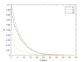
Figure 1: State trajectories of the closed-loop F-16 aircraft system.

Now, we compare the model-free Algorithm 3 with the model-based Algorithm 1. According to Theorem 1, we perform the model-based Algorithm 1 for a sufficiently large number of iterations and utilize the results in the last iteration

$$P^{N+1}=\left[\begin{array}[]{ccc}1.6908&1.3700&-0.1647\\ 1.3700&1.6833&-0.1816\\ -0.1647&-0.1816&0.4372\end{array}\right]$$

as an approximate value of $P^{*}$. To check whether $P^{N+1}$ is the solution of GARE (7), $\mathscr{F}(P^{i+1})$ which is defined in (13) is used to determine the distance from $P^{N+1}$ to the true solution $P^{*}$ of GARE (7). When we insert $P^{N+1}$ into (13), we get

$$\mathscr{F}(P^{N+1})=10^{-16}\times\left[\begin{array}[]{ccc}-4.4409&6.8001&0.0173\\ 2.6368&1.1102&-1.3010\\ -1.0929&0.8153&1.1102\end{array}\right].$$

Since $\left\|\mathscr{F}(P^{N+1})\right\|_{F}=10^{-16}\times 8.8844$ is small enough, we can utilize the results in the last iteration as the optimal values $P^{*}$,$L^{*}$ and $F^{*}$. That is, they can be viewed as the benchmark for the simulation results of Algorithm 3. Fig. 2 depicts the trajectories of the norms of the differences between $\hat{P}^{i},\hat{L}^{i},\hat{F}^{i}$ produced by Algorithm 3 and the optimal values $P^{*},L^{*},F^{*}$.

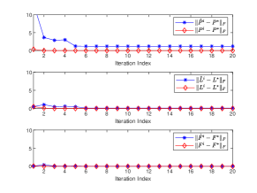
Figure 2: The norms obtained by Algorithm 1 and Algorithm 3.

The above comparison shows that, although the error $\hat{M}^{i}$ induced by the unmeasurable stochastic noise in the system dynamics distorts the trajectories generated by Algorithm 3 from the precise trajectories generated by model-based Algorithm 1, Algorithm 3 still successfully finds a near-optimal control policy. This corresponds to the convergence conclusions achieved in Theorem 4.

7 Conclusions

A data-driven off-policy RL method has been developed to solve stochastic $H_{\infty}$ control problem of continuous-time Itô system with unknown system models. Based on the model-based SPU algorithm, an off-policy RL method is derived, which can learn the solution of GARE from the system data generated by arbitrary control and disturbance signals. The effectiveness of the proposed model-free off-policy RL method is verified by a stochastic linear F-16 aircraft system.

Appendix

Appendix A Proof of Theorem 2

Proof.

(i) Since $P^{*}\succeq 0$ is the stabilizing solution to GARE (7), one has $\sigma\left(\mathscr{L}_{\overline{A}^{*},A_{1}}\right)\subset\mathcal{C}_{-}$ according to Lemma 1, where $\overline{A}^{*}:=\mathscr{A}(P^{*})$. It was shown in Horn  Johnson (2012) that the eigenvalues of a square matrix depend on the matrix elements continuously, thus there always exists a $\bar{\delta}_{0}>0$ such that $\sigma\left(\mathscr{L}_{\overline{A}^{i},A_{1}}\right)\subset\mathcal{C}_{-}$ for all $P^{i}\in\overline{\mathcal{B}}_{\bar{\delta}_{0}}\left(P^{*}\right)$, where $\overline{\mathcal{B}}_{\bar{\delta}_{0}}\left(P^{*}\right)$ is the closure of $\mathcal{B}_{\bar{\delta}_{0}}\left(P^{*}\right)$.

(ii) Suppose $P^{i}\in\overline{\mathcal{B}}_{\bar{\delta}_{0}}\left(P^{*}\right)$ for all $i\in\mathcal{Z}_{+}$. According to (8), the sequence $\left\{P^{i}\right\}_{i=0}^{\infty}$ generated by Algorithm 1 satisfies

$$\mathscr{L}_{\overline{A}^{i},A_{1}}\left(P^{i+1}\right)=-\overline{Q}^{i}.$$ (48)

Based on item (i) of Theorem 2, we have that $\sigma\left(\mathscr{L}_{\overline{A}^{i},A_{1}}\right)$ does not contain zero eigenvalues. According to Lemma 2, $\mathcal{H}\left(\overline{A}^{i},A_{1},H_{n}\right)$ is invertible, and then GLE (8) has a unique real symmetric solution (19).

Subtracting $P^{*}BR^{-1}B^{\top}P^{i}-\gamma^{-2}P^{*}EE^{\top}P^{i}+P^{i}BR^{-1}\\ B^{\top}P^{*}-\gamma^{-2}P^{i}EE^{\top}P^{*}$ from the both sides of GARE (7) with $P=P^{*}$, one has

$$\mathscr{L}_{\overline{A}^{i},A_{1}}\left(P^{*}\right)={P}^{*}\overline{A}^{i}+\left(\overline{A}^{i}\right)^{\top}{P}^{*}+A_{1}^{\top}{P}^{*}A_{1}=-\overline{Q}^{*},$$

where

$$\overline{Q}^{*}= Q+P^{i}BR^{-1}B^{\top}P^{i}-\gamma^{-2}P^{i}EE^{\top}P^{i}$$

$$-\left(P^{i}-P^{*}\right)BR^{-1}B^{\top}\left(P^{i}-P^{*}\right)$$

$$+\gamma^{-2}\left(P^{i}-P^{*}\right)EE^{\top}\left(P^{i}-P^{*}\right).$$

Similar to the process above, we have

$$P^{*}=\left(\mathscr{L}_{\overline{A}^{i},A_{1}}\right)^{-1}\left(-\overline{Q}^{*}\right).$$ (49)

Subtracting (49) from (19), we have

$$\begin{array}[]{l}\operatorname{vecs}\left(P^{i+1}-P^{*}\right)\\ =\mathcal{H}\left(\overline{A}^{i},A_{1},H_{n}\right)^{-1}\operatorname{vecs}\left(\gamma^{-2}\left(P^{i}-P^{*}\right)EE^{\top}\left(P^{i}-P^{*}\right)\right.\\ \left.-\left(P^{i}-P^{*}\right)BR^{-1}B^{\top}\left(P^{i}-P^{*}\right)\right).\end{array}$$

Taking the Euclidean norm for vectors on both sides of the above equation, we have

$$\begin{array}[]{l}\left\|P^{i+1}-P^{*}\right\|_{F}\leq\left\|\mathcal{H}\left(\overline{A}^{i},A_{1},H_{n}\right)^{-1}\right\|_{F}\\ \left\|P^{i}-P^{*}\right\|_{F}^{2}\left[\gamma^{-2}\left\|EE^{\top}\right\|_{F}+\left\|BR^{-1}B^{\top}\right\|_{F}\right].\end{array}$$

By the invertibility of $\mathcal{H}\left(\overline{A}^{i},A_{1},H_{n}\right)$, there exists a $k_{1}>0$ such that $\left\|\mathcal{H}\left(\overline{A}^{i},A_{1},H_{n}\right)^{-1}\right\|_{F}\leq k_{1}$ for all $P^{i}\in\overline{\mathcal{B}}_{\bar{\delta}_{0}}\left(P^{*}\right)$. Then (20) is proved with $k_{0}=k_{1}\left(\gamma^{-2}\left\|EE^{\top}\right\|_{F}+\left\|BR^{-1}B^{\top}\right\|_{F}\right)$. For any $\varepsilon_{0}\in(0,1)$, there exists a $\delta_{0}\in\left(0,\bar{\delta}_{0}\right]$ such that $k_{0}\delta_{0}\leq\varepsilon_{0}$, which proves (21). ∎∎

Appendix B Proof of Theorem 4

We show several supplementary lemmas before showing Theorem 4.

Lemma 7.

For all $\hat{P}^{i}\in\mathcal{B}_{\delta_{0}}\left(P^{*}\right),i\in\mathcal{Z}_{+}$, there exists a $d(\delta_{0})>0$ that is not dependent on $\hat{P}^{i}$, such that if $\|\Delta M^{i}\|_{F}\leq d$, we have that $\sigma\left(\mathscr{L}_{A-B\hat{L}^{i}-E\hat{F}^{i},A_{1}}\right)\subset\mathcal{C}_{-}$ and that $\left[\hat{M}^{i}\right]_{22}$ and $\left[\hat{M}^{i}\right]_{33}$ are invertible.

Proof.

By the same route as item (i) in Theorem 2, it can be shown that $\sigma\left(\mathscr{L}_{\mathscr{A}(\hat{P}^{i}),A_{1}}\right)\subset\mathcal{C}_{-}$ for all $\hat{P}^{i}\in\overline{\mathcal{B}}_{\bar{\delta}_{0}}\left(P^{*}\right)$. Because $\mathscr{A}(P)$ is a continuous function of $P$ and $\overline{\mathcal{B}}_{\bar{\delta}_{0}}\left(P^{*}\right)$ is a compact set, the set $\mathcal{A}:=\left\{\mathscr{A}(\hat{P}^{i})|\hat{P}^{i}\in\overline{\mathcal{B}}_{\bar{\delta}_{0}}\left(P^{*}\right)\right\}$ is also compact. According to the continuity, for each $\hat{P}^{i}\in\overline{\mathcal{B}}_{\bar{\delta}_{0}}\left(P^{*}\right)$, there exists a constant $r>0$ that depends on $\mathscr{A}(\hat{P}^{i})$, such that $\sigma\left(\mathscr{L}_{Y,A_{1}}\right)\subset\mathcal{C}_{-}$ for any $Y\in\mathcal{B}_{r}\left(\mathscr{A}(\hat{P}^{i})\right)$. According to the compactness of $\mathcal{A}$, for all $\hat{P}^{i}\in\overline{\mathcal{B}}_{\bar{\delta}_{0}}\left(P^{*}\right)$, there exists a $\bar{r}>0$ that independs on $\mathscr{A}(\hat{P}^{i})$, such that each $Y\in\mathcal{B}_{\bar{r}}\left(\mathscr{A}\left(\hat{P}^{i}\right)\right)$ satisfies $\sigma\left(\mathscr{L}_{Y,A_{1}}\right)\subset\mathcal{C}_{-}$. It is worth noting that in (45) and (46), the improved policies $\hat{L}^{i}$ and $\hat{F}^{i}$ are continuous functions of $\hat{M}^{i}$. Hence there exists a $d_{1}>0$ such that if $\left\|\Delta M^{i}\right\|_{F}\leq d_{1}$ hods, one has $\left(A-B\hat{L}^{i}-E\hat{F}^{i}\right)\in\mathcal{B}_{\bar{R}}\left(\mathscr{A}\left(\hat{P}^{i}\right)\right)$, and furthermore, $\sigma\left(\mathscr{L}_{A-B\hat{L}^{i}-E\hat{F}^{i},A_{1}}\right)\subset\mathcal{C}_{-}$ for all $\hat{P}^{i}\in\overline{\mathcal{B}}_{\bar{\delta}_{0}}\left(P^{*}\right)$. According to the continuity of the matrix inversion, there exists a $d_{2}>0$ such that $\left[\hat{M}^{i}\right]_{22}$ and $\left[\hat{M}^{i}\right]_{33}$ are invertible if $\|\Delta M^{i}\|_{F}\leq d_{1}$. Letting $d=\min\left(d_{1},d_{2}\right)$ accomplishes the proof.∎∎

According to Lemma 7, if $\|\Delta M\|_{l_{\infty}}\leq d$, then the sequence $\left\{\hat{P}^{i}\right\}_{i=0}^{\infty}$ satisfies (47). The next lemma provides the upper bound of $\left\|\mathcal{D}\left(\overline{M}^{i},\Delta M^{i}\right)\right\|_{F}$.

Lemma 8.

For any $k_{2}>0$, there exist $\delta_{1}^{1}\left(\delta_{0},k_{2}\right)\in(0,d]$ that is independent of $\hat{P}^{i}$ and $k_{3}\left(\delta_{0}\right)>0$, such that if $\left\|\Delta M^{i}\right\|_{F}<\delta_{1}^{1}$, one has

$$\left\|\mathcal{D}\left(\overline{M}^{i},\Delta M^{i}\right)\right\|_{F}\leq k_{3}\left\|\Delta M^{i}\right\|_{F}<k_{2}$$

for all $\hat{P}^{i}\in\mathcal{B}_{\delta_{0}}\left(P^{*}\right)$, where $d$ is defined in Lemma 7.

Proof.

For all $\hat{P}^{i}\in\mathcal{B}_{\delta_{0}}\left(P^{*}\right)$ and $\left\|\Delta M^{i}\right\|_{F}\leq d,i\in\mathcal{Z}_{+}$, according to the continuity of the matrix norm, Proposition 1 and Lemma 7, we have

$$\begin{array}[]{l}\left\|R^{-1}B^{\top}\hat{P}^{i}-\hat{L}^{i}\right\|_{F}\leq\left\|\left[\overline{M}^{i}\right]_{22}^{-1}\right\|_{F}\\ \left(\left\|\Delta M^{i}\right\|_{F}+\left\|\left[\hat{M}^{i}\right]_{22}^{-1}\right\|_{F}\left\|\left[\hat{M}^{i}\right]_{21}\right\|_{F}\left\|\Delta M^{i}\right\|_{F}\right)\\ \leq k_{4}^{1}\left\|\Delta M^{i}\right\|_{F}\end{array}$$ (50)

and

$$\begin{array}[]{l}\left\|-\gamma^{-2}E^{\top}\hat{P}^{i}-\hat{F}^{i}\right\|_{F}\leq\left\|\left[\overline{M}^{i}\right]_{33}^{-1}\right\|_{F}\\ \left(\left\|\Delta M^{i}\right\|_{F}+\left\|\left[\hat{M}^{i}\right]_{33}^{-1}\right\|_{F}\left\|\left[\hat{M}^{i}\right]_{31}\right\|_{F}\left\|\Delta M^{i}\right\|_{F}\right)\\ \leq k_{4}^{2}\left\|\Delta M^{i}\right\|_{F}\end{array}$$ (51)

for some $k_{4}^{1}\left(\delta_{0},d\right)>0,k_{4}^{2}\left(\delta_{0},d\right)>0$. Define

$$\Delta X_{i}= \mathcal{H}\left(\hat{\overline{A}}^{i},A_{1},H_{n}\right)-\mathcal{H}\left(A-B\hat{L}^{i}-E\hat{F}^{i},A_{1},H_{n}\right),$$

$$\Delta Y_{i}= \operatorname{vecs}\left(\hat{Q}^{i}_{2}-\hat{Q}^{i}_{1}\right).$$

Noting (50) and (51), it is easy to check that $\left\|\Delta X_{i}\right\|_{F}\leq k_{5}\left\|\Delta M^{i}\right\|_{F},\left\|\Delta Y_{i}\right\|_{2}\leq k_{6}\left\|\Delta M^{i}\right\|_{F}$ for some $k_{5}\left(\delta_{0},d\right)>0$ and $k_{6}\left(\delta_{0},d\right)>0$. Then according to the continuity of the matrix norm, Lemma 2 and Proposition 1, one has

$$\begin{array}[]{l}\left\|\mathcal{D}\left(\overline{M}^{i+1},\Delta M^{i+1}\right)\right\|_{F}\\ \leq\left\|\mathcal{H}\left(A-B\hat{L}^{i}-E\hat{F}^{i},A_{1},H_{n}\right)^{-1}\right\|_{F}\left\|\Delta M^{i}\right\|_{F}\\ \left\{k_{6}+k_{5}\left\|\mathcal{H}\left(\hat{\overline{A}}^{i},A_{1},H_{n}\right)^{-1}\right\|_{F}\right.\\ \left.\left[\left\|-\hat{P}^{i}BR^{-1}B^{\top}\hat{P}^{i}\right\|_{F}+\left\|\gamma^{-2}\hat{P}^{i}EE^{\top}\hat{P}^{i}\right\|_{F}\right]\right\}\\ \leq k_{3}\left(\delta_{0}\right)\left\|\Delta M^{i}\right\|_{F}.\end{array}$$

Taking $0<\delta_{1}^{1}\leq d$ with $k_{3}\delta_{1}^{1}<k_{2}$ completes the proof. ∎∎

Now we are in a position to prove Theorem 4.

Proof.

Let $k_{2}=(1-\varepsilon_{0})\delta_{0}$ in Lemma 8 and $\delta_{1}=\delta_{1}^{1}\left(\delta_{0},k_{2}\right)$. For any $i\in\mathcal{Z}_{+}$, if $\hat{P}^{i}\in\mathcal{B}_{\delta_{0}}\left(P^{*}\right)$, then

$$\left\|\hat{P}^{i+1}-P^{*}\right\|_{F}$$

$$\leq \left\|\left(\mathscr{L}_{\hat{\overline{A}}^{i},A_{1}}\right)^{-1}\left(-\hat{Q}^{i}_{1}\right)-P^{*}\right\|_{F}+\left\|\mathcal{D}\left(\overline{M}^{i},\Delta M^{i}\right)\right\|_{F}$$

$$\leq \varepsilon_{0}\left\|\hat{P}^{i}-P^{*}\right\|_{F}+k_{3}\left\|\Delta M^{i}\right\|_{F}$$ (52)

$$\leq \varepsilon_{0}\left\|\hat{P}^{i}-P^{*}\right\|_{F}+k_{3}\|\Delta M\|_{l_{\infty}}$$ (53)

$$< \varepsilon_{0}\delta_{0}+k_{3}\delta_{1}<\varepsilon_{0}\delta_{0}+k_{2}=\delta_{0},$$ (54)

where (52) and (54) hold because of Theorem 2 and Lemma 8. By induction, (52) – (54) hold for all $i\in\mathbb{Z}_{+}$, therefore (i) in Theorem 4 is proved. As a result, according to (52), one has

$$\left\|\hat{P}^{i}-P^{*}\right\|_{F}$$

$$\leq \varepsilon_{0}^{2}\left\|\hat{P}^{i-2}-P^{*}\right\|_{F}+(\varepsilon_{0}+1)k_{3}\|\Delta M\|_{l_{\infty}}$$

$$\leq \cdots$$

$$\leq \varepsilon_{0}^{i}\left\|\hat{P}^{0}-P^{*}\right\|_{F}+\left(1+\cdots+\varepsilon_{0}^{i-1}\right)k_{3}\|\Delta M\|_{l_{\infty}}$$

$$< \varepsilon_{0}^{i}\left\|\hat{P}^{0}-P^{*}\right\|_{F}+\frac{k_{3}}{1-\varepsilon_{0}}\|\Delta M\|_{l_{\infty}},$$

which proves (ii) in Theorem 4. As to (iii) in Theorem 4, for any $\varepsilon>0$, there exists a $i_{1}\in\mathcal{Z}_{+}$ such that $\sup\left\{\left\|\Delta M^{i}\right\|_{F}\right\}_{i=i_{1}}^{\infty}<\beta^{-1}(\varepsilon/2)$. Let $i_{2}\geq i_{1}$, for $k\geq i_{2}$, because $\hat{P}^{i}$ is bounded, in accordance with (ii) in Theorem 4, we have

$$\left\|\hat{P}^{i}-P^{*}\right\|_{F} \leq\alpha\left(\left\|\hat{P}^{i_{2}}-P^{*}\right\|_{F},i-i_{2}\right)+\varepsilon/2$$

$$\leq\alpha\left(k_{7},i-i_{2}\right)+\varepsilon/2,$$

for some $k_{7}\left(\delta_{0},d\right)>0$. Because $\lim_{i\rightarrow\infty}\alpha\left(k_{7},i-i_{2}\right)=0$, there is a $i_{3}\geq i_{2}$ such that $\alpha\left(k_{7},i-i_{2}\right)<\varepsilon/2$ for all $i\geq i_{3}$, which completes the proof.∎∎

References

• Başar \BBA Bernhard (\APACyear1995) \APACinsertmetastarbacsar1995h{APACrefauthors}Başar, T.\BCBT \BBA Bernhard, P.  \APACrefYear1995. \APACrefbtitle${H}_{\infty}$-Optimal Control and Related Minimax Design Problems: A dynamic game approach ${H}_{\infty}$-optimal control and related minimax design problems: A dynamic game approach. \APACaddressPublisherBirkhäuser. \PrintBackRefs\CurrentBib
• Berger (\APACyear1977) \APACinsertmetastarberger1977nonlinearity{APACrefauthors}Berger, M\BPBIS.  \APACrefYear1977. \APACrefbtitleNonlinearity and functional analysis: Lectures on nonlinear problems in mathematical analysis Nonlinearity and functional analysis: Lectures on nonlinear problems in mathematical analysis. \APACaddressPublisherAcademic Press. \PrintBackRefs\CurrentBib
• Bertsekas (\APACyear2019) \APACinsertmetastarbertsekas2019reinforcement{APACrefauthors}Bertsekas, D.  \APACrefYear2019. \APACrefbtitleReinforcement learning and optimal control Reinforcement learning and optimal control. \APACaddressPublisherAthena Scientific. \PrintBackRefs\CurrentBib
• Bian \BOthers. (\APACyear2016) \APACinsertmetastarbian2016adaptive{APACrefauthors}Bian, T., Jiang, Y.\BCBL \BBA Jiang, Z\BHBIP.  \APACrefYearMonthDay2016. \BBOQ\APACrefatitleAdaptive dynamic programming for stochastic systems with state and control dependent noise Adaptive dynamic programming for stochastic systems with state and control dependent noise.\BBCQ \APACjournalVolNumPagesIEEE Transactions on Automatic Control61124170–4175. \PrintBackRefs\CurrentBib
• Chen \BBA Zhang (\APACyear2004) \APACinsertmetastarchen2004stochastic{APACrefauthors}Chen, B\BHBIS.\BCBT \BBA Zhang, W.  \APACrefYearMonthDay2004. \BBOQ\APACrefatitleStochastic ${H}_{2}/{H}_{\infty}$ Control with State-dependent Noise Stochastic ${H}_{2}/{H}_{\infty}$ control with state-dependent noise.\BBCQ \APACjournalVolNumPagesIEEE Transactions on Automatic Control49145–57. \PrintBackRefs\CurrentBib
• Damm (\APACyear2002) \APACinsertmetastardamm2002state{APACrefauthors}Damm, T.  \APACrefYearMonthDay2002. \BBOQ\APACrefatitleState-feedback ${H}_{\infty}$ -type control of linear systems with time-varying parameter uncertainty State-feedback ${H}_{\infty}$ -type control of linear systems with time-varying parameter uncertainty.\BBCQ \APACjournalVolNumPagesLinear Agebra and its Applications351185–210. \PrintBackRefs\CurrentBib
• Doyal \BOthers. (\APACyear1989) \APACinsertmetastardoyal1989state{APACrefauthors}Doyal, J., Glover, K., Khargoneker, P.\BCBL \BBA Francis, B.  \APACrefYearMonthDay1989. \BBOQ\APACrefatitleState space solutions to standard ${H}_{2}/{H}_{\infty}$ control problems State space solutions to standard ${H}_{2}/{H}_{\infty}$ control problems.\BBCQ \APACjournalVolNumPagesIEEE Transactions on Automatic Control348831–847. \PrintBackRefs\CurrentBib
• Dragan \BBA Ivanov (\APACyear2011) \APACinsertmetastardragan2011computation{APACrefauthors}Dragan, V.\BCBT \BBA Ivanov, I\BPBIG.  \APACrefYearMonthDay2011. \BBOQ\APACrefatitleComputation of the stabilizing solution of game theoretic Riccati equation arising in stochastic ${H}_{\infty}$ control problems Computation of the stabilizing solution of game theoretic Riccati equation arising in stochastic ${H}_{\infty}$ control problems.\BBCQ \APACjournalVolNumPagesNumerical Algorithms573357–375. \PrintBackRefs\CurrentBib
• Dragan \BOthers. (\APACyear2006) \APACinsertmetastardragan2006mathematical{APACrefauthors}Dragan, V., Morozan, T.\BCBL \BBA Stoica, A\BHBIM.  \APACrefYear2006. \APACrefbtitleMathematical methods in robust control of linear stochastic systems Mathematical methods in robust control of linear stochastic systems (\BVOL 50). \APACaddressPublisherSpringer. \PrintBackRefs\CurrentBib
• Feng \BBA Anderson (\APACyear2010) \APACinsertmetastarfeng2010iterative{APACrefauthors}Feng, Y.\BCBT \BBA Anderson, B\BPBID.  \APACrefYearMonthDay2010. \BBOQ\APACrefatitleAn iterative algorithm to solve state-perturbed stochastic algebraic Riccati equations in LQ zero-sum games An iterative algorithm to solve state-perturbed stochastic algebraic Riccati equations in LQ zero-sum games.\BBCQ \APACjournalVolNumPagesSystems $\&$ Control Letters59150–56. \PrintBackRefs\CurrentBib
• Hinrichsen \BBA Pritchard (\APACyear1998) \APACinsertmetastarhinrichsen1998stochastic{APACrefauthors}Hinrichsen, D.\BCBT \BBA Pritchard, A\BPBIJ.  \APACrefYearMonthDay1998. \BBOQ\APACrefatitleStochastic ${H}_{\infty}$ Stochastic ${H}_{\infty}$.\BBCQ \APACjournalVolNumPagesSIAM Journal on Control and Optimization3651504–1538. \PrintBackRefs\CurrentBib
• Horn \BBA Johnson (\APACyear2012) \APACinsertmetastarhorn2012matrix{APACrefauthors}Horn, R\BPBIA.\BCBT \BBA Johnson, C\BPBIR.  \APACrefYear2012. \APACrefbtitleMatrix analysis Matrix analysis. \APACaddressPublisherCambridge University Press. \PrintBackRefs\CurrentBib
• Kiumarsi \BOthers. (\APACyear2017) \APACinsertmetastarkiumarsi2017optimal{APACrefauthors}Kiumarsi, B., Vamvoudakis, K\BPBIG., Modares, H.\BCBL \BBA Lewis, F\BPBIL.  \APACrefYearMonthDay2017. \BBOQ\APACrefatitleOptimal and autonomous control using reinforcement learning: A survey Optimal and autonomous control using reinforcement learning: A survey.\BBCQ \APACjournalVolNumPagesIEEE Transactions on Neural Networks and Learning Systems2962042–2062. \PrintBackRefs\CurrentBib
• Krylov (\APACyear1995) \APACinsertmetastarkrylov1995introduction{APACrefauthors}Krylov, N\BPBIV.  \APACrefYearMonthDay1995. \BBOQ\APACrefatitleIntroduction to the theory of diffusion processes Introduction to the theory of diffusion processes.\BBCQ \APACjournalVolNumPagesAmerican Mathematical Society8585–600. \PrintBackRefs\CurrentBib
• Lanzon \BOthers. (\APACyear2008) \APACinsertmetastarlanzon2008computing{APACrefauthors}Lanzon, A., Feng, Y., Anderson, B\BPBID.\BCBL \BBA Rotkowitz, M.  \APACrefYearMonthDay2008. \BBOQ\APACrefatitleComputing the positive stabilizing solution to algebraic Riccati equations with an indefinite quadratic term via a recursive method Computing the positive stabilizing solution to algebraic Riccati equations with an indefinite quadratic term via a recursive method.\BBCQ \APACjournalVolNumPagesIEEE Transactions on Automatic Control53102280–2291. \PrintBackRefs\CurrentBib
• Li \BOthers. (\APACyear2022) \APACinsertmetastarli2022stochastic{APACrefauthors}Li, N., Li, X., Peng, J.\BCBL \BBA Xu, Z\BPBIQ.  \APACrefYearMonthDay2022. \BBOQ\APACrefatitleStochastic linear quadratic optimal control problem: A reinforcement learning method Stochastic linear quadratic optimal control problem: A reinforcement learning method.\BBCQ \APACjournalVolNumPagesIEEE Transactions on Automatic Control6795009–5016. \PrintBackRefs\CurrentBib
• Pang \BOthers. (\APACyear2021) \APACinsertmetastarpang2021robust{APACrefauthors}Pang, B., Bian, T.\BCBL \BBA Jiang, Z\BHBIP.  \APACrefYearMonthDay2021. \BBOQ\APACrefatitleRobust policy iteration for continuous-time linear quadratic regulation Robust policy iteration for continuous-time linear quadratic regulation.\BBCQ \APACjournalVolNumPagesIEEE Transactions on Automatic Control671504–511. \PrintBackRefs\CurrentBib
• Pang \BBA Jiang (\APACyear2023) \APACinsertmetastarpang2022reinforcement{APACrefauthors}Pang, B.\BCBT \BBA Jiang, Z\BHBIP.  \APACrefYearMonthDay2023. \BBOQ\APACrefatitleReinforcement learning for adaptive optimal stationary control of linear stochastic systems Reinforcement learning for adaptive optimal stationary control of linear stochastic systems.\BBCQ \APACjournalVolNumPagesIEEE Transactions on Automatic Control6842383–2390. \PrintBackRefs\CurrentBib
• Rall (\APACyear1974) \APACinsertmetastarrall1974note{APACrefauthors}Rall, L.  \APACrefYearMonthDay1974. \BBOQ\APACrefatitleA note on the convergence of Newton’s method A note on the convergence of Newton’s method.\BBCQ \APACjournalVolNumPagesSIAM Journal on Numerical Analysis11134–36. \PrintBackRefs\CurrentBib
• Stevens \BOthers. (\APACyear2015) \APACinsertmetastarstevens2015aircraft{APACrefauthors}Stevens, B\BPBIL., Lewis, F\BPBIL.\BCBL \BBA Johnson, E\BPBIN.  \APACrefYear2015. \APACrefbtitleAircraft control and simulation: Dynamics, controls design, and autonomous systems Aircraft control and simulation: Dynamics, controls design, and autonomous systems. \APACaddressPublisherJohn Wiley & Sons. \PrintBackRefs\CurrentBib
• Sutton \BBA Barto (\APACyear1999) \APACinsertmetastarsutton1999reinforcement{APACrefauthors}Sutton, R\BPBIS.\BCBT \BBA Barto, A\BPBIG.  \APACrefYearMonthDay1999. \BBOQ\APACrefatitleReinforcement learning: An introduction Reinforcement learning: An introduction.\BBCQ \APACjournalVolNumPagesRobotica172229–235. \PrintBackRefs\CurrentBib
• Tapia (\APACyear1971) \APACinsertmetastartapia1971kantorovich{APACrefauthors}Tapia, R.  \APACrefYearMonthDay1971. \BBOQ\APACrefatitleThe Kantorovich Theorem for Newton’s method The Kantorovich Theorem for Newton’s method.\BBCQ \APACjournalVolNumPagesThe American Mathematical Monthly784389–392. \PrintBackRefs\CurrentBib
• van der Schaft (\APACyear1992) \APACinsertmetastarvan19922{APACrefauthors}van der Schaft, A\BPBIJ.  \APACrefYearMonthDay1992. \BBOQ\APACrefatitle${L}_{2}$-gain analysis of nonlinear systems and nonlinear state feedback ${H}_{\infty}$ control ${L}_{2}$-gain analysis of nonlinear systems and nonlinear state feedback ${H}_{\infty}$ control.\BBCQ \APACjournalVolNumPagesIEEE Transactions on Automatic Control376770–784. \PrintBackRefs\CurrentBib
• Wei \BOthers. (\APACyear2023) \APACinsertmetastarwei2023continuous{APACrefauthors}Wei, Q., Zhou, T., Lu, J., Liu, Y., Su, S.\BCBL \BBA Xiao, J.  \APACrefYearMonthDay2023. \BBOQ\APACrefatitleContinuous-time stochastic policy iteration of adaptive dynamic programming Continuous-time stochastic policy iteration of adaptive dynamic programming.\BBCQ \APACjournalVolNumPagesIEEE Transactions on Systems, Man, and Cybernetics: Systems53106375–6387. \PrintBackRefs\CurrentBib
• Willems \BOthers. (\APACyear2005) \APACinsertmetastarwillems2005note{APACrefauthors}Willems, J\BPBIC., Rapisarda, P., Markovsky, I.\BCBL \BBA De Moor, B\BPBIL.  \APACrefYearMonthDay2005. \BBOQ\APACrefatitleA note on persistency of excitation A note on persistency of excitation.\BBCQ \APACjournalVolNumPagesSystems $\&$ Control Letters544325–329. \PrintBackRefs\CurrentBib
• Wu \BBA Luo (\APACyear2013) \APACinsertmetastarwu2013simultaneous{APACrefauthors}Wu, H\BHBIN.\BCBT \BBA Luo, B.  \APACrefYearMonthDay2013. \BBOQ\APACrefatitleSimultaneous policy update algorithms for learning the solution of linear continuous-time ${H}_{\infty}$ state feedback control Simultaneous policy update algorithms for learning the solution of linear continuous-time ${H}_{\infty}$ state feedback control.\BBCQ \APACjournalVolNumPagesInformation Sciences222472–485. \PrintBackRefs\CurrentBib
• Zames (\APACyear1981) \APACinsertmetastarzames1981feedback{APACrefauthors}Zames, G.  \APACrefYearMonthDay1981. \BBOQ\APACrefatitleFeedback and optimal sensitivity: Model reference transformations, multiplicative seminorms, and approximate inverses Feedback and optimal sensitivity: Model reference transformations, multiplicative seminorms, and approximate inverses.\BBCQ \APACjournalVolNumPagesIEEE Transactions on Automatic Control262301–320. \PrintBackRefs\CurrentBib
• Zhang \BBA Chen (\APACyear2004) \APACinsertmetastarzhang2004stabilizability{APACrefauthors}Zhang, W.\BCBT \BBA Chen, B\BHBIS.  \APACrefYearMonthDay2004. \BBOQ\APACrefatitleOn stabilizability and exact observability of stochastic systems with their applications On stabilizability and exact observability of stochastic systems with their applications.\BBCQ \APACjournalVolNumPagesAutomatica40187–94. \PrintBackRefs\CurrentBib
• Zhang \BBA Chen (\APACyear2012) \APACinsertmetastarzhang2012cal{APACrefauthors}Zhang, W.\BCBT \BBA Chen, B\BHBIS.  \APACrefYearMonthDay2012. \BBOQ\APACrefatitle$\mathscr{H}$-Representation and Applications to Generalized Lyapunov Equations and Linear Stochastic Systems $\mathscr{H}$-representation and applications to generalized Lyapunov equations and linear stochastic systems.\BBCQ \APACjournalVolNumPagesIEEE Transactions on Automatic Control57123009–3022. \PrintBackRefs\CurrentBib
• Zhang \BOthers. (\APACyear2017) \APACinsertmetastarzhang2017stochastic{APACrefauthors}Zhang, W., Xie, L.\BCBL \BBA Chen, B\BHBIS.  \APACrefYear2017. \APACrefbtitleStochastic ${H}_{2}/{H}_{\infty}$ control: A Nash game approach Stochastic ${H}_{2}/{H}_{\infty}$ control: A Nash game approach. \APACaddressPublisherCRC Press. \PrintBackRefs\CurrentBib