Unbiased Markov chain quasi-Monte Carlo for Gibbs samplers

Abstract

In statistical analysis, Monte Carlo (MC) stands as a classical numerical integration method. When encountering challenging sample problem, Markov chain Monte Carlo (MCMC) is a commonly employed method. However, the MCMC estimator is biased after a fixed number of iterations. Unbiased MCMC, an advancement achieved through coupling techniques, addresses this bias issue in MCMC. It allows us to run many short chains in parallel. Quasi-Monte Carlo (QMC), known for its high order of convergence, is an alternative of MC. By incorporating the idea of QMC into MCMC, Markov chain quasi-Monte Carlo (MCQMC) effectively reduces the variance of MCMC, especially in Gibbs samplers. This work presents a novel approach that integrates unbiased MCMC with MCQMC, called as an unbiased MCQMC method. This method renders unbiased estimators while improving the rate of convergence significantly. Numerical experiments demonstrate that unbiased MCQMC with a sample size of $N$ achieves convergence rates of approximately $O(N^{-1})$ in moderate dimensions for Gibbs sampling problems. In the setting of parallelization, unbiased MCQMC also performs better than unbiased MCMC, even running with short chains.

1 Introduction

As widely known, Monte Carlo (MC) method is utilized to estimate the expectation $E_{\pi}[f(X)]$ for a target distribution $\pi$ with respect to a certain function $f$. Over the past few decades, MC has been widely applied in diverse fields such as science, engineering, finance, industry, and statistical inference [11, 34]. In practical applications, MC requires sampling from the target distribution. In cases where direct sampling from the target distribution is not feasible, such as the posterior distribution in Bayesian computation, one often resorts to Markov chain Monte Carlo (MCMC) method. In MCMC, a Markov chain is simulated, and sample averages are used to estimate the expectation of the target distribution. Classical MCMC algorithms include Metropolis-Hastings (MH) samplers and Gibbs samplers [37]. For any MCMC algorithm, as the number of iterations increases, sample averages converge to the expectation with probability 1 (w.p.1), i.e.,

$$\frac{1}{N}\sum\limits_{i=1}^{N}f(X_{i})\stackrel{{\scriptstyle w.p.1}}{{\to}}E_{\pi}[f(X)],$$

where $N$ is the sample size, and $(X_{t})_{t\geq 0}$ is a Markov chain with $\pi$ as its stationary distribution. This ensures the consistency of MCMC algorithms.

However, for a fixed number of iterations, if the Markov chain is initialized from a state outside the stationary distribution, it is uncertain when the chain will enter the stationary distribution. Consequently, the obtained samples always contain a portion that does not follow the stationary distribution, leading to a bias known as “burn-in bias”. This bias presents challenges for the parallelization of MCMC and has prompted the development of various methods, such as the coupling method proposed by Nicholls et al. [28], and circularly-coupled Markov chain proposed by Neal [27]. Recently, Glynn and Rhee [12] utilized coupling techniques to entirely eliminate the mean bias of the Markov chain traversal average as represented by iterative stochastic functions. Jacob et al. [19] eliminated the bias of conditional particle filters by using coupling chains. Jacob et al. [20] then proposed an unbiased MCMC method, which results in unbiased estimators for MH samplers and Gibbs samplers. Unbiased MCMC enables highly parallelized MCMC algorithms, making them widely applicable in various fields such as likelihood-free Bayesian inference [25], hardware acceleration [24], and more.

Another limitation of MC in practical applications is due to its slow root mean square error (RMSE) rate $O(N^{-1/2}$) for $N$ samples. This rate also holds for MCMC and unbiased MCMC. To improve MC, one may use deterministic low-discrepancy sequences instead of independent and identically distributed (IID) random sequences, known as quasi-Monte Carlo (QMC) methods [7, 31]. For a $d$-dimensional integral, QMC yields deterministic error bounds of $O(N^{-1}(\log N)^{d})$ for certain regular functions, which are asymptotically superior to MC rate $O(N^{-1/2})$. In practice, randomized QMC (RQMC) is more frequently used. It preserves the low discrepancy property of QMC and enables error estimation via several replications. Randomization methods such as random shifts [5], digital shifts [35], and scrambling [32] are commonly utilized in RQMC. QMC and RQMC have been successfully used in finance and statistics [17, 23, 42].

Given the advantages of QMC over MC, it is worthwhile to consider the idea of replacing IID sequences in MCMC processes with deterministic sequences. However, directly substituting typical low-discrepancy sequences with IID sequences may not produce correct results. This is due to the fact that deterministic low-discrepancy sequences exhibit strong correlations, which disrupt the Markov property of the Markov chain in the MCMC process, as discussed in [39, Section 3.2]. Therefore, another type of uniform sequences is required. Motivated by Niederreiter [30], Owen and Tribble [36, 40] proposed Markov chain quasi-Monte Carlo (MCQMC) method. They have proved that using completely uniformly distributed (CUD) or weakly CUD (WCUD) sequences in discrete spaces can yield consistent results. Chen et al. [3] extended these consistency results to continuous spaces. For properties related to (W)CUD sequences, we refer to [30, 40]. (W)CUD sequences are sequences of infinite length, but in practical applications, it is necessary to work with finite (W)CUD sequences, called as array-(W)CUD sequences. Several methods have been developed for designing array-(W)CUD sequences. These methods include Liao’s method [21], Multiplicative Congruential Generator (MCG) method [29, 36, 40], and Linear Feedback Shift Register (LFSR) generators over the two-element field $\mathbb{F}_{2}$ [4, 13, 39] and LFSR generators over the four-element field $\mathbb{F}_{4}$ [14]. While it is difficult to theoretically rank the effectiveness of these generators, existing experimental results in [13, 14] suggest that, LFSR generators proposed by Harase [13, 14] exhibit the best performance for specific sample sizes in most cases. Moreover, experimental results in [14] show that the difference in performance between the generators in [13] and [14] is not significant, but the generators in [13] enable more sample selections. In this paper, we refer to the generators in [13] as Harase’s method, and utilize Harase’s method for specific sample sizes. Furthermore, by taking advantage of the feature of Liao’s method that does not impose specific constraints on sample sizes, we utilize Liao’s method to fulfill the flexibility in sample sizes.

Currently, the theoretical foundations for determining the convergence rate of MCQMC are weak. Under the assumptions that the update function being a strong contracting mapping and the real-valued function $f$ is sufficiently regular, Chen [2] proved that for any $\epsilon>0$, MCQMC exhibits a convergence order similar to QMC methods, i.e., $O(N^{-1+\epsilon})$. However, this result does not represent a typical absolute error for all samples mean and the required sequence is related to the strong contracting condition. Liu [22] applied Chen’s convergence theory to Langevin diffusion models. She attributed the partial error of MCQMC to systematic error. If we ignore the systematic error, this work obtained the absolute error convergence order of all samples mean as $O(N^{-1+\epsilon})$. Dick et al. [8, 9] presented a Koksma-Hlawka inequality for MCQMC. Under relatively weak conditions, they demonstrated the existence of a driving sequence achieving a convergence rate for MCQMC of $O(N^{-1/2}(\log N)^{1/2})$. Furthermore, if the update function satisfies the “anywhere-to-anywhere” condition, there exists a driving sequence that results in a convergence rate of $O(N^{-1+\epsilon})$.

Apart from the limited theoretical guarantees for MCQMC, many experimental results in the literature indicate the effective performance of MCQMC, especially in Gibbs samplers. For example, it was observed in [13] that Harase’s method yields several orders of magnitude reduction in variance. These findings motivate us to integrate unbiased MCMC with MCQMC, with the goal of preserving the unbiasedness of MCMC estimators while simultaneously reducing the variance of the estimators. To this end, we propose a method of unbiased MCQMC for Gibbs samplers. The unbiased MCQMC method is beyond a mere amalgamation of unbiased MCMC and MCQMC. The challenges involved include determining how to effectively utilize array-(W)CUD sequences in unbiased MCMC to enhance the performance of MCQMC. Moreover, we should note that the chains generated with array-(W)CUD sequences are no longer Markovian, which implies that certain properties associated with unbiased MCMC may not be applied to unbiased MCQMC.

In unbiased MCMC, given the chains of length $N$, we independently run the chains $R$ times to obtain $R$ estimators, and the final estimator is the average of $R$ estimators. Therefore, in fact, the convergence order of unbiased MCMC is $O(N^{-1/2}R^{-1/2})$. In Section 4, we demonstrate that the convergence rate of unbiased MCQMC is equivalent to that of MCQMC, which means that the convergence order of unbiased MCMC may be $O(N^{-1+\epsilon}R^{-1/2})$. The purpose of unbiased MCMC is to achieve highly parallel execution, maintaining a small $N$ and running $R$ short chains in parallel instead of running long chains as in MCMC. Benefiting from the unbiased estimators on each chain and the linearity of $R$ in computational budget, by increasing $R$, we can obtain high precision in a relatively short time. When parallel resources are limited, the benefits for unbiased MCMC of running long chains or repeating multiple chains within the same budget are equivalent. But, benefiting from the convergence order of unbiased MCQMC, $O(N^{-1+\epsilon})$, running longer chains can achieve higher precision within the same budget. Conversely, when parallel resources are abundant, for a fixed small $N$, the convergence orders of unbiased MCMC and unbiased MCQMC are both $O(R^{-1/2})$. But, intuitively and as numerical experiments demonstrate, unbiased MCQMC can parallelize shorter chains than unbiased MCMC to achieve a given precision.

The contribution of this paper is three-fold. Firstly, we introduce the unbiased MCQMC method by integrating unbiased MCMC and MCQMC. This method requires the use of array-(W)CUD sequences in the partial sampling process of unbiased MCMC. The construction of array-(W)CUD sequences resembles pseudo-random numbers and does not involve additional computational complexity. Secondly, we theoretically establish the upper bounds on the second moment of the bias term in unbiased MCQMC without relying on the Markov property and the geometric drift condition, which were required in [20]. Lastly, we prove the unbiasedness of the proposed methods. Numerical experiments across various dimensions demonstrate the convergence rate of unbiased MCQMC for Gibbs sampling problems is $O(N^{-1+\epsilon})$ for any $\epsilon>0$. When $N$ is large, the variance reduction is significant. On the other hand, in the setting of parallelization, unbiased MCQMC can save several times the sample size to achieve the similar efficiency of unbiased MCMC.

The paper is organized as follows. Section 2 provides a brief introduction to QMC, MCMC, MCQMC, and unbiased MCMC. Section 3 presents a comprehensive framework for the unbiased MCQMC method, and shows the influence of parameters selection and the performance of unbiased MCQMC through a toy example. Section 4 establishes the consistency and unbiasedness of the estimator in unbiased MCQMC, accompanied by a discussion of the estimator’s variance. Section 5 provides numerical experiments on the performance of unbiased MCQMC for different dimensional Gibbs samplers. The conclusion is presented in Section 6. A lengthy proof is put in Appendix A.

2 Background

2.1 Quasi-Monte Carlo

QMC is a deterministic version of MC, known for its higher order rate of convergence compared to MC. Here, we provide a brief introduction to QMC, and further information can be found in the monographs [7, 31].

QMC is commonly used for the numerical integration of $d$-dimensional integral $\mu=\int_{(0,1)^{d}}f(\mathbf{u})\mathrm{d}\mathbf{u}$. The estimator is represented as $\hat{\mu}=\frac{1}{N}\sum_{i=1}^{N}f(\bm{u}_{i})$, where $\bm{u}_{i}\in(0,1)^{d}$. In comparison to MC, where $\bm{u}_{i}$ are IID, $\{\bm{u}_{i}\}_{i=1}^{N}$ used in QMC are low-discrepancy points. The discrepancy of a point set is typically quantified using the star discrepancy, which is defined by

$$D_{N}^{*}\left(\bm{u}_{1},\ldots,\bm{u}_{N}\right)=\sup_{\bm{z}\in(0,1)^{d}}\left|\frac{1}{N}\sum_{i=1}^{N}1_{\left\{\bm{u}_{i}\in[\mathbf{0},\mathbf{z})\right\}}-\prod_{j=1}^{d}z_{j}\right|.$$ (1)

A point set with a star discrepancy of $O(N^{-1}(\log N)^{d})$ is referred to as a low-discrepancy point set. Commonly used QMC point sets include Sobol’ sequences, Faure sequences, Halton sequences, lattice rules, and others. The star discrepancy plays a crucial role in determining the estimation error of integrals over $(0,1)^{d}$. The classical Koksma-Hlawka inequality provides an error bound, i.e.,

$$|\hat{\mu}-\mu|\leq D_{N}^{*}\left(\bm{u}_{1},\ldots,\bm{u}_{N}\right)V_{\mathrm{HK}}(f),$$ (2)

where $V_{\mathrm{HK}}(\cdot)$ is the variation (in the sense of Hardy and Krause) of a function. For the definition and properties of $V_{\mathrm{HK}}(\cdot)$, we refer to [33]. To facilitate error estimation, RQMC is commonly used. Typical randomization methods include random shifts [5], digital shifts [35] and scrambling [32].

2.2 Markov chain Monte Carlo

MCMC extends the scope of MC. In this section, following [3, Section 2.4], we shall briefly introduce MCMC by update functions. Given the target distribution $\pi$ on $\Omega\subseteq\mathbb{R}^{d}$, our goal is to sample $X\sim\pi$ and approximate $\theta(f)=\int f(x)\pi(x)dx$. Consider a Markov chain $(X_{t})_{t\geq 0}$ with $P$ as its transition kernel and an update function $\phi$ such that $\pi$ is a stationary distribution for $(X_{t})_{t\geq 0}$. We start by an arbitrary $X_{0}\in\Omega$ with $\pi(X_{0})>0$, and then, for $i\geq 1$, the state updating process is defined as $X_{i}\sim P(X_{i-1},\cdot)=\phi(X_{i-1},\bm{u}_{i})$, where $\bm{u}_{i}\sim U(0,1)^{d}$. Then we estimate $\theta(f)$ by $\frac{1}{N}\sum_{i=1}^{N}f(X_{i})$. If a burn-in period are required, we assume that $X_{0}$ is the last sample point of it. The update functions for the Gibbs sampler are shown in the following.

Sequential Scan Gibbs Update. Let the current state be ${\mathbf{x}}=(\mathbf{x}_{1},\ldots,\mathbf{x}_{s})\in\Omega$ with $\mathbf{x}_{i}\in\mathbb{R}^{k_{i}}$ and $d=\sum_{i=1}^{s}k_{i}$ and $\psi({\mathbf{x}_{-i}},\cdot):(0,1)^{k_{i}}\to\mathbb{R}$ be a $k_{i}$-dimensional generator of the full conditional distribution of $\mathbf{x}_{i}$ given $\mathbf{x}_{j}$ for all $j\neq i$. For $\mathbf{u}=(\mathbf{u}_{1},\ldots,\mathbf{u}_{s})\in(0,1)^{d}$ with $\mathbf{u}_{i}\in(0,1)^{k_{i}}$, the next state ${\mathbf{y}}$ can be given by

$$\mathbf{y}=\phi\left(\mathbf{x},\mathbf{u}\right)=\left(\phi_{1}\left(\mathbf{x},\mathbf{u}_{1}\right),\phi_{2}\left(\mathbf{x},\mathbf{u}_{2}\right),\ldots,\phi_{s}\left(\mathbf{x},\mathbf{u}_{s}\right)\right),$$ (3)

where $\phi_{i}\left(\mathbf{x},\mathbf{u}\right)=\psi({\mathbf{x}_{-i}},\mathbf{u}_{i})$ and $\mathbf{x}_{-i}=\left(\phi_{1}\left(\mathbf{x},\mathbf{u}_{1}\right),\ldots,\phi_{i-1}\left(\mathbf{x},\mathbf{u}_{i-1}\right),\mathbf{x}_{i+1},\ldots,\mathbf{x}_{s}\right)$, $i=1,2,\ldots,s.$

Here, we transform the process of sampling random variables into functions of uniform random variables, which involves how to generate non-uniform random variables using uniform random variables. To this end, we resort to the quantile functions of the non-uniform random variables [6, 34].

2.3 Markov chain quasi-Monte Carlo

Replacing IID $U(0,1)$ points with carefully designed sequences in MCMC is expected to yield more accurate estimates. In this section, we review MCQMC by following the introduction in [39, Chapter 3].

Suppose we want to collect $N$ samples, each requiring $d$ uniform variables. The required uniform variables can be organized into a variable matrix as follows,

$$\left[\begin{array}[]{cccc}v_{1}&v_{2}&\cdots&v_{d}\\ v_{d+1}&v_{d+2}&\cdots&v_{2d}\\ \vdots&\vdots&\ddots&\vdots\\ v_{(N-1)d+1}&v_{(N-1)d+2}&\cdots&v_{Nd}\end{array}\right],$$ (4)

where $v_{i}\stackrel{{\scriptstyle iid}}{{\sim}}U(0,1)$. The sequence $(v_{1},v_{2},\ldots,v_{Nd})$ is referred to as the “driving sequence” of MCMC. The driving sequence should be designed carefully with certain uniformity in MCQMC. In this paper, (W)CUD sequences defined below are used as driving sequences.

Definition 1.

An infinite sequence $(v_{i})_{i\geq 1}$ in $(0,1)$ is called as a CUD sequence if for any $d\geq 1$,

$$D_{N}^{*}\left((v_{1},\ldots,v_{d}),(v_{2},\ldots,v_{d+1}),\ldots,(v_{N},\ldots,v_{N+d})\right)\to 0,\text{~{}as~{}}N\to\infty,$$

where $D_{N}^{*}$ is defined in (1). An infinite sequence $(v_{i})_{i\geq 1}$ in $(0,1)$ is called as a WCUD sequence if for any $\epsilon>0$ and $d\geq 1$,

$$\mathbb{P}\left(D_{N}^{*}\left((v_{1},\ldots,v_{d}),(v_{2},\ldots,v_{d+1}),\ldots,(v_{N},\ldots,v_{N+d})\right)>\epsilon\right)\to 0,\text{~{}as~{}}N\to\infty.$$

In practice, we use finite (W)CUD sequences. So the triangular array (W)CUD sequences is more useful. A triangular array $(v_{N,1},v_{N,2},\ldots,v_{N,N})$ for $N$ in an infinite positive integers set $\mathscr{N}$ is called as array-CUD, if for any $d\geq 1$, as $N\to\infty$ through the values in $\mathscr{N}$,

$$D_{N-d+1}^{*}\left((v_{N,1},\ldots,v_{N,d}),(v_{N,2},\ldots,v_{N,d+1}),\ldots,(v_{N,N-d+1},\ldots,v_{N,N})\right)\to 0.$$ (5)

Array-WCUD is defined analogously.

We focus on Liao’s method [21] and Harase’s method [13] in this work. Liao’s method is to randomize the order of the given $d$-dimensional QMC sequences, which does not need specific constraints on the sample size. Therefore, in our unbiased MCQMC method, we utilize Liao’s method to care for any sample size. For LFSR generators, [13] emphasized that it essentially possesses a digital net structure. For sequences with digital net structures, the t-value serves as a critical optimization metric. We shall use LFSR generators over $\mathbb{F}_{2}$ optimized for the t-value for specific sample sizes.

2.4 Unbiased Markov chain Monte Carlo

By using coupling techniques, Jacob et al.[20] proposed the unbiased MCMC method to addresses this bias issue in MCMC. In this section, we follow [20] to construct an unbiased estimator for $E_{\pi}[f(X)]$. Let $P$ be the Markov transition kernel on $\Omega$ with $\pi$ as its stationary distribution, and let $\bar{P}$ be a transition kernel on the joint space $\Omega\times\Omega$. Consider two Markov chains $(X_{t})_{t\geq 0}$ and $(Y_{t})_{t\geq 0}$ with $\pi_{0}$ as their initial distribution. Initially, two independent samples $X_{0}$ and $Y_{0}$ are drawn from $\pi_{0}$. Following this, given $X_{0}$, the sample $X_{1}$ is drawn from $P$. Then, for $t\geq 1$, given the pair $(X_{t},Y_{t-1})$, the pair $(X_{t+1},Y_{t})$ is drawn from $\bar{P}$. Assume that $\bar{P}$ is a coupling kernel for $(X_{t})_{t\geq 0}$ and $(Y_{t})_{t\geq 0}$, satisfying $X_{t+1}|(X_{t},Y_{t-1})\sim P(X_{t},\cdot)$ and $Y_{t}|(X_{t},Y_{t-1})\sim P(Y_{t-1},\cdot)$. Thus, for any $t\geq 0$, $X_{t}$ and $Y_{t}$ follow identical distributions. Moreover, the design of the coupling kernel $\bar{P}$ ensures the existence of a random variable referred to as the meeting time $\tau$, such that for any $t\geq\tau$, $X_{t}=Y_{t-1}$. Hence, for a given integer $k\geq 0$, we have

$$E_{\pi}[f(X)]=\lim\limits_{t\to\infty}E[f(X_{t})] =E[f(X_{k})]+\sum_{l=k+1}^{\infty}E[f(X_{l})]-E[f(X_{l-1})]$$ (6)

$$=E\left[f(X_{k})+\sum_{l=k+1}^{\infty}\{f(X_{l})-f(Y_{l-1})\}\right]$$

$$=E\left[f(X_{k})+\sum_{l=k+1}^{\tau-1}\{f(X_{l})-f(Y_{l-1})\}\right].$$

If $\tau-1<k+1$, $\sum_{l=k+1}^{\tau-1}\{f(X_{l})-f(Y_{l-1})\}$ is zero by convention. Therefore, an unbiased estimator of $E_{\pi}[f(X)]$ is given by

$$F_{k}(\bm{X},\bm{Y}):=f(X_{k})+\sum_{l=k+1}^{\tau-1}\{f(X_{l})-f(Y_{l-1})\},$$

where $\bm{X}$ and $\bm{Y}$ represent two coupled Markov chains $(X_{t})_{t\geq 0}$ and $(Y_{t})_{t\geq 0}$. Furthermore, for a given integer $m\geq k$, consider the unbiased estimator formed by the average of $m-k+1$ unbiased estimators $F_{l}(\bm{X},\bm{Y})$, where $l=k,k+1,\ldots,m$. It follows that

$$F_{k:m}(\bm{X},\bm{Y}) :=\frac{1}{m-k+1}\sum_{l=k}^{m}F_{l}(\bm{X},\bm{Y})$$ (7)

$$=\frac{1}{m-k+1}\sum_{l=k}^{m}f(X_{l})+\sum_{l=k+1}^{\tau-1}\min\!\left(1,\frac{l-k}{m-k+1}\right)\{f(X_{l})-f(Y_{l-1})\}$$

$$=:\text{MCMC}_{k:m}+\text{BC}_{k:m}.$$

When considering $(X_{t})_{t\geq 0}$ only, it is a standard Markov chain. The first term $\text{MCMC}_{k:m}$ in (7) can be interpreted as the average value of the standard Markov chain after $m$ iterations, with a burn-in period of $k$. Clearly, it is biased. Thus, the second term $\text{BC}_{k:m}$ in (7) can be considered as a bias correction term. To obtain the unbiased estimator (7), it is necessary to know that how to construct the specific coupling kernel $\bar{P}$ and how to sample from $\bar{P}$. Following [20], we consider the maximal coupling method. The maximal coupling of distributions $p$ and $q$ on the space $\Omega$ is the joint distribution of the random variables $(Z,Z^{\prime})$. This distribution satisfies the marginal distributions $Z\sim p$ and $Z^{\prime}\sim q$, and it maximizes the probability of the event $\{Z=Z^{\prime}\}$.

By incorporating the array-(W)CUD sequences in unbiased MCMC, we have successfully accelerated the convergence speed of unbiased MCMC with MCQMC. In the following, we provide the construction of the unbiased MCQMC method in detail, along with some theoretical results.

3 Unbiased Markov chain quasi-Monte Carlo

In unbiased MCMC, we construct two Markov chains, while MCQMC deals with only one chain. When applying MCQMC to unbiased MCMC, a fundamental question arises. Which chain’s IID sequence should be replaced with a (W)CUD sequence —– only dealing with $(X_{t})_{t\geq 0}$, only dealing with $(Y_{t})_{t\geq 0}$, or both $(X_{t})_{t\geq 0}$ and $(Y_{t})_{t\geq 0}$? Combined with MCMC and MCQMC, we describe the sample process of unbiased MCMC as driven by two variable matrices. For easy of notation, we rewrite the sample process as follows, which is a combination of Algorithms 1 and 2 for Gibbs sampler in [20].

Algorithm 1 Unbiased estimator $F_{k:m}(\bm{X},\bm{Y})$ of $E_{\pi}[f(X)]$ by IID sequences for Gibbs sampler

1:  Given $\pi_{0}$, update function $\phi$ defined in (3) and conditional density $P_{i},i=1,2,\ldots,s$ of the components of each part with $d=\sum_{i=1}^{s}k_{i}.$

2:  Sample $X_{0},Y_{0}\sim\pi_{0}$, and $V\sim U(0,1)^{d}$, set $X_{1}=\phi(X_{0},V)$, $t=1,\tau=\infty$

3:  Repeat steps 4-13 until $t\geq\max(m,\tau)$

4:  if $t<\tau$ then

5:     for $i$ in $1$ to $s$ do

6:        Set $p_{i}(\cdot)=P_{i}(X_{t,-i},\cdot),q_{i}(\cdot)=P_{i}(Y_{t,-i},\cdot)$, sample $v\sim U(0,1)^{k_{i}}$ and $w\sim U(0,1)$, set $X_{t,i}=\psi_{i}(X_{t,-i},v)$ and $W|X_{t,i}=p_{i}(X_{t,i})w$

7:        If $W\leq q_{i}(X_{t,i})$, set $Y_{t,i}=X_{t,i}$, otherwise, sample $v\sim U(0,1)^{k_{i}}$ and $w\sim U(0,1)$, set $Y_{t,i}=\psi_{i}(Y_{t,-i},v)$, and $W|Y_{t,i}=q_{i}(Y_{t,i})w$ until $W>p_{i}(Y_{t,i})$

8:     end for

9:     Set $X_{t+1}=X_{t},Y_{t}=Y_{t-1}$. If $X_{t+1}=Y_{t}$, set $\tau=t$, $t=t+1$

10:  else

11:     Sample $V\sim U(0,1)^{d}$, set $X_{t+1}=\phi(X_{t},V)$, $Y_{t}=X_{t+1}$ and $t=t+1$

12:  end if

13:  Return $F_{k:m}(\bm{X},\bm{Y})$ by (7)

For the chain $(X_{t})_{t\geq 0}$, its variable matrix is

$$V_{X}=\left[{\begin{array}[]{*{4}{c}}{v_{1}^{(X)}}&{v_{2}^{(X)}}&\cdots&{v_{d}^{(X)}}\\ {v_{d+1}^{(X)}}&{v_{d+2}^{(X)}}&\cdots&{v_{2d}^{(X)}}\\ \vdots&\vdots&\ddots&\vdots\\ {v_{{(M-1)d+1}}^{(X)}}&{v_{{(M-1)d+2}}^{(X)}}&\cdots&{v_{{Md}}^{(X)}}\end{array}}\right],$$

where $M=\max(m,\tau)$ and $v_{i}^{(X)}\stackrel{{\scriptstyle iid}}{{\sim}}U(0,1)$. Denote $A$ as

$$\left[{\begin{array}[]{*{20}{c}}{{w_{1,1}}}&{v_{1,1}^{(Y)}}&{v_{1,2}^{(Y)}}&\cdots&{v_{1,d}^{(Y)}}&{{w_{1,2}}}&{\left({\begin{array}[]{*{20}{c}}{v_{1,d+1}^{(Y)}}&{v_{1,d+2}^{(Y)}}&\cdots&{v_{1,2d}^{(Y)}}&{{w_{1,3}}}\end{array}}\right)}&\cdots\\ {{w_{2,1}}}&{v_{2,1}^{(Y)}}&{v_{2,2}^{(Y)}}&\cdots&{v_{2,d}^{(Y)}}&{{w_{2,2}}}&{\left({\begin{array}[]{*{20}{c}}{v_{2,d+1}^{(Y)}}&{v_{2,d+2}^{(Y)}}&\cdots&{v_{2,2d}^{(Y)}}&{{w_{2,3}}}\end{array}}\right)}&\cdots\\ \vdots&\vdots&\vdots&\ddots&\vdots&\vdots&\vdots&\vdots\\ {{w_{T,1}}}&{v_{T,1}^{(Y)}}&{v_{T,2}^{(Y)}}&\cdots&{v_{T,d}^{(Y)}}&{{w_{T,2}}}&{\left({\begin{array}[]{*{20}{c}}{v_{T,d+1}^{(Y)}}&{v_{T,d+2}^{(Y)}}&\cdots&{v_{T,2d}^{(Y)}}&{{w_{T,3}}}\end{array}}\right)}&\cdots\\ {{w_{\tau,1}}}\end{array}}\right],$$

where $T=\tau-1$, $w_{i,j},v_{i,j}^{(Y)}\stackrel{{\scriptstyle iid}}{{\sim}}U(0,1)$. For the chain $(Y_{t})_{t\geq 0}$, its variable matrix $V_{Y}=[V_{X}|A]$.

In practice, when using array-(W)CUD sequences, it is necessary to determine the length of the sequences in advance. Given $d$ and $m$, the number of columns in $V_{X}$ is fixed, but the number of rows in $V_{X}$ is related to the random variable $\tau$. Fortunately, since it takes the maximum value of $m$ and $\tau$, we can set the number of rows of the variable matrix driven by an array-(W)CUD sequence to be $m$. If the selected $m<\tau$, we use an IID sequence with an unspecified length to fill in the gap. In Section 4.1, we will demonstrate the rationality behind this approach. Nevertheless, the number of rows and columns in $V_{Y}$ is uncertain. In the maximum coupling algorithm, the sampling of $(Y_{t})_{t\geq 0}$ is similar to acceptance-rejection sampling. The number of variables needed for each update is uncertain. Additionally, the number of rows in $V_{Y}$ is $\tau$, which makes it impossible to handle $V_{Y}$ in the same way as $V_{X}$. Hence, we do not modify the sampling process of $(Y_{t})_{t\geq 0}$.

It is worth noting that in the sampling process of $(X_{t})_{t\geq 0}$, directly replacing IID sequences with array-(W)CUD sequences is inappropriate when $k>1$. In unbiased MCMC, if we have some knowledge about the meeting time $\tau$ via simulations, [20] suggested that choosing $k$ as a large quantile of $\tau$. On the other hand, although they did not use burn-in periods in their experiments, the majority of authors in [3, 13, 22, 40] recommended to use (W)CUD sequences on MCQMC with a burn-in period because doing otherwise would compromise the overall uniformity of (W)CUD sequences. Therefore, $k$, or the burn-in period, is necessary and valuable in unbiased MCQMC. We propose to use an IID sequence before the $(k-1)$-th step for convenience, as the sample sizes of Harase’s method are fixed and the samples generated in the previous $k$ steps are not needed. This allows for a flexible choice of $k$. Next we provide a toy example to illustrate the influence of $k$ in unbiased MCQMC and the effect of directly using array-(W)CUD sequences versus using array-(W)CUD sequences after the $(k-1)$-th step.

Normal Gibbs sampler. This toy example is a systematic Gibbs sampler to generate the $d$-dimensional multivariate normal distribution $\mathbf{X}\sim\pi=\mathcal{N}(\bm{\mu}$, $\bm{\Sigma})$ which can be implemented as

$$X_{i}\mid\mathbf{X}_{-i}\sim\mathcal{N}(\bm{\mu}_{i}+\bm{\Sigma}_{i,-i}\bm{\Sigma}_{-i,-i}^{-1}(\mathbf{X}_{-i}-\bm{\mu}_{-i}),~{}\bm{\Sigma}_{i,i}-\bm{\Sigma}_{i,-i}\bm{\Sigma}_{-i,-i}^{-1}\bm{\Sigma}_{-i,i}),$$

for $i=1,2,\ldots,d$, where $-i$ denotes the vector $(1,2,\ldots,i-1,i+1,\ldots,d)$ and $\bm{\Sigma}_{-i,-i}$ denotes the sub-matrix of $\bm{\Sigma}$ whose rows are in $-i$ and columns are in $-i$. For $d$-dimensional Normal variable $Q_{1}\sim\mathcal{N}(\bm{\mu}$, $\bm{\Sigma})$, we have $Q_{1}=\bm{\mu}+\bm{C}\Phi^{-1}(V)$, where $\bm{C}\bm{C}^{T}=\bm{\Sigma}$, $V\sim U(0,1)^{d}$ and $\Phi^{-1}(\cdot)$ is the quantile function of the standard normal distribution [34]. Hence, the update function for each parameters of this model is clear. Set $d=3$ and

$$\mu=\left({\begin{array}[]{*{20}{c}}0\\ 0\\ 0\end{array}}\right),\Sigma=\left({\begin{array}[]{*{20}{c}}1&{0.7}&{0.4}\\ {0.7}&1&{0.6}\\ {0.4}&{0.6}&1\end{array}}\right),$$

which was used in [39, Chapter 6.1]. We estimate $E[X_{1}]$, $E[X_{2}]$ and $E[X_{3}]$, whose true values are all $0$. At first, we consider the case of directly using array-(W)CUD sequences. After $5000$ simulations by IID sequences and Harase’s method, we get the histograms of $\tau$ in Figure 1.

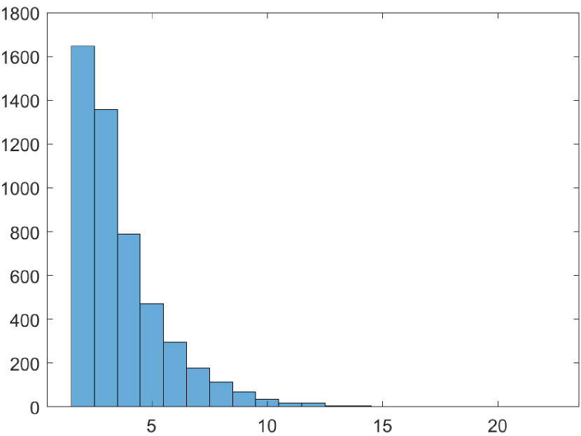
(a) IID sequences.

(b) Harase’s method.

Figure 1: Histogram of $\tau$ in 3-dimensional multivariate normal distribution.

We can see that the distributions of $\tau$ obtained by IID sequences or Harase’s method are similar. Their $99.9\%$ quantile are around $15$. This phenomenon is also observed in other experiments, suggesting that using array-(W)CUD sequences may not affect the distribution of $\tau$. Hence, in the following experiments, we only provide the $\tau$ values obtained from IID sequences.

Let $m=k+N-1$, where $N$ is the sample size used for estimation. We consider $k=1,15,20,25$ to examine the influence of $k$ in unbiased MCQMC. Moreover, we consider using Harase’s method after the $(k-1)$-th step with $k=15$. The reduction factors of RMSE for unbiased MCQMC estimating $E[X_{1}]$ relative to unbiased MCMC are provided in Table 1. The results for $E[X_{2}]$ and $E[X_{3}]$ are similar.

Table 1: The reduction factors (RF) of RMSE for estimating $E[X_{1}]$ via unbiased MCQMC driven by Harase’s method.

$E[X_{1}]$		$N=2^{10}$		$N=2^{13}$		$N=2^{16}$
		IID-RMSE	RF	IID-RMSE	RF	IID-RMSE	RF
Case 1	$k=15$	3.99E-05	512	4.50E-06	4782	6.16E-07	31968
Case 2	$k=1$	3.63E-03	15	4.71E-04	106	4.35E-05	483
	$k=15$	3.70E-05	100	4.37E-06	939	4.25E-07	4414
	$k=20$	3.83E-05	66	4.38E-06	684	4.25E-07	3140
	$k=25$	3.85E-05	56	4.37E-06	531	4.25E-07	2168

In Table 1, “Case 1” denotes the use of Harase’s method after the $(k-1)$-th step, while “Case 2” represents directly using Harase’s method. “IID-RMSE” indicates the RMSE of unbiased MCMC, and “RF” indicates the RMSE reduction factors of unbiased MCQMC driven by Harase’s method with respect to unbiased MCMC. The results are provided for $N=2^{10}$, $2^{13}$, $2^{16}$.

Due to the $99.9$% quantile of $\tau$ is $15$, when $k\geq 15$, the bias correction term is almost negligible. Indeed, we observe that for Case 2, when $k\geq 15$, the RMSE variation of unbiased MCMC is minimal as it is induced by a slight change in the sample sizes. Conversely, the RMSE reduction factor variation of unbiased MCQMC is substantial and decreases with $k$. This implies that with an increasing $k$, i.e., more points discarded from an array-(W)CUD sequence, overall uniformity is more severely disrupted, resulting in a larger RMSE for the sample mean. However, if we completely retain the array-(W)CUD sequence, the performance is not satisfactory. In Case 2, with $k=1$, the bias correction term cannot be ignored. Interestingly, it can be observed that the bias correction term with a small number of samples has a minimal impact on the RMSE of unbiased MCMC but significantly diminishes the performance of unbiased MCQMC. In contrast, when choosing $k$ to be a large quantile of $\tau$ and using an array-(W)CUD sequence after the $(k-1)$-th step, we can achieve better performance with unbiased MCQMC. We will explain this phenomenon later. Therefore, the approach of using array-(W)CUD sequences after the $(k-1)$-th step is helpful. Going forward, we refer to this approach as the unbiased MCQMC method. Then, we present the RMSE convergence plot for the unbiased MCQMC mehtod in Figure 2.

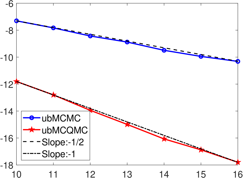
(a) $E[X_{1}]$.

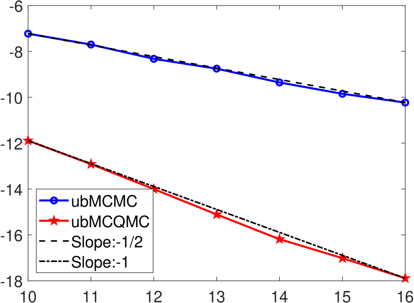
(b) $E[X_{2}]$.

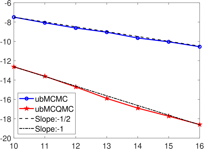
(c) $E[X_{3}]$.

Figure 2: RMSEs (on a $\log_{2}$ scale) of ubMCMC and ubMCQMC for estimating $E[X_{i}],i=1,2,3$.

The vertical axis corresponds to $\log_{2}(\text{RMSE})$ and the horizontal axis corresponds to $\log_{2}(N)$. “ubMCMC” presents the unbiased MCMC method, and “ubMCQMC” presents the unbiased MCQMC method. We observe from Figure 2 that the RMSE rate of ubMCQMC is $O(N^{-1})$ beating the $O(N^{-1/2})$ rate of ubMCMC. It is worth noting that if we switch to unbiased MCQMC driven by Liao’s method, similar properties are observed, including sensitivity to $k$ and a convergence rate of $O(N^{-1})$. But, Harase’s method exhibits superior performance, as described in Introduction.

In the aforementioned experiments, we observe that the correction bias term has a minor impact in unbiased MCMC but a significant impact in unbiased MCQMC. By Proposition 3 in [20], we know that the square root of the second moment for the bias correction term in unbiased MCMC has an order of $O(N^{-1})$, while the order of the RMSE for traditional MCMC is $O(N^{-1/2})$. Therefore, in unbiased MCMC, the dominant term in RMSE is the first term $\text{MCMC}_{k:m}$ in (7). By Proposition 2, we conclude that the order of the square root of the second moment for the bias correction term in unbiased MCQMC is also $O(N^{-1})$. Additionally, based on existing numerical experiments in MCQMC for Normal Gibbs sampler model [2, 13, 39], the order of RMSE for MCQMC is approximately $O(N^{-1})$. In Figure 2, we also observe that the order of RMSE for unbiased MCQMC is approximately $O(N^{-1})$. Therefore, it is reasonable to conclude that $\text{BC}_{k:m}$ is of the same order as $\text{MCMC}_{k:m}$ in unbiased MCQMC for this model, which explains why the bias correction term has such a significant impact on the RMSE results in unbiased MCQMC.

Note that the introduction of unbiased MCMC was aimed at achieving parallelization, i.e., maintaining a small $N$ and running $R$ short chains in parallel instead of long chains as in MCMC. For example, in the experiments of [20, Section 5.1], for $k=200$, $m$ may take $4000$ to be sufficient compared to the efficiency of traditional MCMC long chains. We will discuss the performance of unbiased MCQMC in the parallelized setting later. Now, we need to address another issue: how to achieve arbitrary sample requirements in unbiased MCQMC as in unbiased MCMC?

Flexible Sample Size.  The number of rows in the matrix generated by Harase’s method is $N=2^{n}$ (add a row of all 0s), where $10\leq n\leq 32$, and it is not extensible. This constrains the choice of $m$, and we are unable to generate samples for the sizes $N\neq 2^{n},n=10,11,\ldots,32$. In contrast, Liao’s method [21] works with arbitrary sample sizes. Therefore, when $N\neq 2^{n},n=10,11,\ldots,32$, we can directly use Liao’s method. Moreover, when $2^{n}<N<2^{n+1},n=10,11,\ldots,31$ and $N>2^{32}$, considering the scheme in the sampling process of $(X_{t})_{t\geq 0}$, an alternative method is to initially utilize Harase’s method with a length of $2^{n}$ and then use an IID sequence or Liao’s method with a length of $N-2^{n}$ to fill in the remaining gap. We refer to these two methods as “Harase-IID” method and “Harase-Liao” method, respectively. We compare three methods for the aforementioned toy model. We choose Sobol’ sequence [38] as the QMC sequence used in Liao’s method. To emphasize flexibility, the length of Sobol’ sequence is arbitrarily chosen and is neither a prime number nor a power of two as commonly used. Let $m=n_{e}+N+k-1$, where $N$ is the length of Harase’s method and $n_{e}$ is the number of additional samples needed to reach $m$ based on $N$ and $k$. We set $k=15$, $N=2^{i},i=10,11$. For each $N$, we consider $n_{e}=0,50,200,500,1000$. Additionally, we also take $m-k+1=50,200,500,1000$. In Figure 3, the vertical axis corresponds to $\log_{2}(\text{RMSE})$, and the horizontal axis corresponds to $m-k+1$.

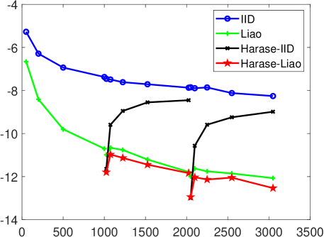
Figure 3: RMSEs (on a $\log_{2}$ scale) for estimating $E[X_{1}]$ with different sample sizes.

From Figure 3, it is clear that Liao’s method have good results for any sample size. Moreover, it performs better when the sample sizes are powers of 2. But, the improvement is not as good as the Harase-Liao method, especially in $m-k+1=2^{n}$. On the other hand, as the sample size increases, the gain of the Harase-IID method gradually decreases, approaching the IID method, but it still outperforms the IID method. Among these methods, the Harase-Liao method stands out as the most effective. Although there is currently no definitive theoretical judgment on the superiority of array-(W)CUD sequences, (10) in Theorem 1 shows that as the sample size of the inferior sequence in the combination of two array-(W)CUD sequences increases, the star discrepancy of the combined sequence will approach that of the inferior sequence. Figure 3 intuitively suggests that if we assume that an array-(W)CUD sequence exhibits better performance with smaller star discrepancy in any dimension, then the effect of the combined sequence will become comparable to that of the inferior sequence. Combining the performance shown in Figure 3, for convenience, we use Harase’s method for $m-k+1=2^{n}$, $10\leq n\leq 32$, and we use Liao’s method with Sobol’ sequence for other sample sizes.

The core of unbiased MCMC lies in utilizing the property that estimators on each chain are unbiased and the linearity of $R$ in the computational budget, allowing for high precision in a relatively short time by increasing $R$. However, when parallel resources are limited, for unbiased MCMC, the benefits of running long chains or repeating multiple chains are similar. However, at this point, benefiting from the convergence order of unbiased MCQMC, which is $O(N^{-1+\epsilon}R^{-1/2})$, running longer chains can achieve higher precision within the same budget. Below, we use the normal Gibbs model to illustrate this point.

The so-called parallel resources are limited, meaning that there are a fixed number of chains that can be run in parallel. Taking a CPU with 24 cores as an example, which is capable of running $24$ chains simultaneously. If we want to obtain $96000$ samples, there are several choices available: $N\times R=100\times 960=1000\times 96=4000\times 24$. For unbiased MCMC, these choices are equivalent, with the theoretical cost time required being $C(NR)/24$ where $C$ denotes the cost time to generate one sample and the RMSE is $C_{1}(NR)^{-1/2}$. For unbiased MCQMC, since the construction of array-(W)CUD sequences resembles pseudo-random numbers, the RMSE will be $C_{2}N^{-1+\epsilon}R^{-1/2}$ with any $\epsilon>0$ at the same cost time, where $C_{1},C_{2}$ are constants independent of $N$ and $R$. Table 2 shows the effect of different choices of $N$ and $R$ for unbiased MCMC and unbiased MCQMC estimating $E[X_{1}]$ in the normal Gibbs model. In all cases, $k=15$. “RF” indicates the RMSE reduction factors of unbiased MCQMC with respect to unbiased MCMC in the same choice. The longer cost time of the third choice may be attributed to the fact that communication between chains during parallel execution also requires time. It is clear that for unbiased MCMC, the benefits of these choices are equivalent. But for unbiased MCQMC, under the same choices, it can achieve higher precision compared to unbiased MCMC, and the option with longer chains yields better benefits.

Table 2: The effect of different choices of $N$ and $R$ for unbiased MCMC and unbiased MCQMC estimating $E[X_{1}]$.

$E[X_{1}]$		unbiased MCMC				unbiased MCQMC
$N\times R$		$4000\times 24$	$1000\times 96$	$100\times 960$		$4000\times 24$	$1000\times 96$	$100\times 960$ [t]
Time(s)		0.38	0.38	0.44		0.38	0.38	0.44
RMSE		6.26E-03	6.32E-03	6.07E-03		3.11E-04	5.91E-04	1.68E-03
RF		-	-	-		20.17	10.69	3.62[b]

Next, we use the same model to demonstrate that when parallel resources are abundant, for a fixed and small $N$, unbiased MCQMC can parallelize shorter chains than unbiased MCMC to achieve the efficiency of MCMC estimators. Following [20], to compare the efficiency of $F_{k:m}(\bm{X},\bm{Y})$ in unbiased MCMC and unbiased MCQMC and that of MCMC estimators, we define the asymptotic inefficiency of $F_{k:m}(\bm{X},\bm{Y})$ as the product of its variance and its expected cost, which can be explained by the asymptotic variance of the estimator as the computational budget tends to infinity. Since the construction of array-(W)CUD sequences resembles pseudo-random numbers, the cost of estimators $F_{k:m}(\bm{X},\bm{Y})$ in unbiased MCQMC is the same as in unbiased MCMC, both being $2(\tau-1)+\max(1,m+1-\tau)$ iterations of the underlying MCMC algorithm. For $m\geq k$, when $k$ increases, we expect $(m-k+1)\text{MSE}_{k:m}$ to converge to

$$V_{k:m}:=V\left[(m+k-1)^{-1/2}\sum\limits_{t=k}^{m}f(X_{t})\right]$$

with $X_{t}\sim\pi$. The limit of $V_{k:m}$ as $m\to\infty$ denoted by $V_{\infty}$ is the asymptotic variance of the MCMC estimator. We assume that $(m-k+1)\text{MSE}_{k:m}\approx V_{\infty}$ for $k$ large enough. The loss of efficiency of the method compared with standard MCMC methods is defined by

$$E\left[2(\tau-1)+\max(1,m+1-\tau)\right]\times V[F_{k:m}(\bm{X},\bm{Y})]/V_{\infty}.$$

As discussed in [20, Section 3.1], when $k$ and $m$ are sufficiently large, the loss of efficiency for unbiased MCMC is close to $1$, meaning that the variance brought by the unbiasedness can be eliminated by choosing sufficiently large $k$ and $m$. However, in the setting of parallelization, one might prefer to keep $k$ and $m$ relatively small to achieve a suboptimal efficiency, but generate more independent estimators within a given computing time.

For the normal Gibbs model with $k=15$ and considering different choices of $m$, we run $1000$ the chains in parallel to obtain $1000$ estimators and values of $\tau$. Utilizing these, we estimate the expected cost $E[2(\tau-1)+\max(1,m+1-\tau)]$ and the variance of the estimators. Meanwhile, the asymptotic variance of MCMC is obtained from $1000$ long chains with $5\times 10^{5}$ iterations and $10^{3}$ burn-in periods. The expected cost, the variance of estimators, and the loss of efficiency of unbiased MCMC and unbiased MCQMC are given in Table 3. We see that for $k=15,m=150$, i.e., $N=136$, the efficiency of unbiased MCMC is comparable to that of standard MCMC methods. However, For unbiased MCQMC, to obtain efficiency comparable to standard MCMC methods, we just require $k=15,m=23$, i.e., $N=9$, resulting in a reduction of sample size by a factor of $136/9\approx 15$.

Table 3: Cost, variance and the loss of efficiency for unbiased MCMC and unbiased MCQMC estimating $E[X_{1}]$.

$E[X_{1}]$	$k$	$m$	Cost	Variance	Inefficiency/$V_{\infty}$
ubMCMC	15	30	32.73	2.00E-04	1.7919 [t]
	15	75	67.73	6.49E-05	1.2019
	15	150	152.73	2.50E-05	1.0434 [b]
ubMCQMC	15	20	22.72	2.40E-04	1.4880 [t]
	15	23	25.72	1.48E-04	1.0409
	15	25	27.72	1.23E-04	0.9357 [b]

4 Convergence analysis

In this section, we first demonstrate that the aforementioned concatenation of array-(W)CUD sequences remains an array-(W)CUD sequence, ensuring the consistency of the proposed Harase-Liao and Harase-IID methods. We then prove the unbiasedness of the proposed estimator and discuss its variance.

4.1 The consistency of the Harase-Liao and Harase-IID methods

We know that when replacing IID sequences in the MCMC sampling process with other sequences, it is preferable to use (W)CUD sequences, theoretically ensuring consistency [3, 40]. In the aforementioned process of selecting the row number in the variable matrix and making arbitrary choices for $m$, we utilize the concatenation of different array-(W)CUD sequences. This raises a question: Does the concatenated sequence retain the array-(W)CUD property? If not, this approach is risky. Theorem 1 answers this question, establishing that the naturally concatenated sequence of two array-(W)CUD sequences remains an array-(W)CUD sequence. To prove Theorem 1, we begin by presenting a useful lemma introduced in Lemma 3.2.3 of [39].

Lemma 4.1.

The sequence $(v_{i})_{i\geq 1}$ is CUD if and only if for arbitrary integers $1\leq l\leq d$, the sequence $\{\mathbf{z}_{i}\}$ defined by $\mathbf{z}_{i}=(v_{id-l+1},v_{id-l+2},\ldots,v_{(i+1)d-l})$ satisfies

$$\lim\limits_{n\to\infty}D_{N}^{*}(\mathbf{z}_{1},\mathbf{z}_{2},\ldots,\mathbf{z}_{N})=0,~{}\text{as}~{}N\to\infty.$$

where $D_{N}^{*}$ is the star discrepancy defined in (1). An analogous equivalence holds for WCUD sequences.

Lemma 4.1 illustrates that (W)CUD sequences exhibit good balance not only for overlapping blocks but also for non-overlapping blocks with any offset. The result of this lemma also holds for array-(W)CUD as shown in [39].

Theorem 1.

Suppose that $(v_{N,1},v_{N,2},\ldots,v_{N,N})$ and $(u_{M,1},u_{M,2},\ldots,u_{M,M})$ are two array-(W)CUD sequences, then $(w_{T,1},w_{T,2},\ldots,w_{M,T})$ is also an array-(W)CUD sequence with $T=N+M$ and $w_{T,i}=v_{N,i},w_{T,N+j}=u_{M,j},\ i=1,2,\ldots,N,\ j=1,2,\ldots,M$.

Proof.

We only consider the array-CUD sequence, and the proof of the array-WCUD sequence is similar. By the definition of array-CUD sequences given in (5), for any $d\geq 1$, as $N\to\infty$ through the values in an infinite positive integers set $\mathscr{N}$, we have

$$D_{N-d+1}^{*}\left((v_{N,1},\ldots,v_{N,d}),(v_{N,2},\ldots,v_{N,d+1}),\ldots,(v_{N,N-d+1},\ldots,v_{N,N})\right)\to 0.$$

By Lemma 4.1 with $l=d$, it is equivalent to

$$D_{N^{\prime}}^{*}\left(\mathbf{x}_{1},\mathbf{x}_{2},\ldots,\mathbf{x}_{N^{\prime}}\right)\to 0,~{}\text{as}~{}N^{\prime}\to\infty,$$ (8)

where $\mathbf{x}_{i}=(v_{N,(i-1)d+1},v_{N,(i-1)d+2},\ldots,v_{N,id}),\ i=1,2,\ldots,N^{\prime}$ and $N^{\prime}=\lfloor N/d\rfloor$. Similarly, by Lemma 4.1 with $l=N\mod d$, we also have

$$D_{M^{\prime}}^{*}\left(\mathbf{y}_{1},\mathbf{y}_{2},\ldots,\mathbf{y}_{M^{\prime}}\right)\to 0,~{}\text{as}~{}M^{\prime}\to\infty,$$ (9)

where $\mathbf{y}_{j}=(u_{M,jd-l+1},u_{M,jd-l+2},\ldots,u_{M,jd-l+d}),\ j=1,2,\ldots,M^{\prime}$ and $M^{\prime}=\lfloor(M-d+l)/d\rfloor$. Let $\mathbf{z}=(v_{N,N^{\prime}d+1},v_{N,N^{\prime}d+2},\ldots,v_{N,N},u_{M,1},u_{M,2},\ldots,u_{M,d-l})$, and $T^{\prime}=M^{\prime}+N^{\prime}+1$. By the definition of star discrepancy given in (1) and absolute value inequality, it is easy to obtain that

$$D_{T^{\prime}}^{*}\left(\mathbf{x}_{1},\mathbf{x}_{2},\ldots,\mathbf{x}_{N^{\prime}},\mathbf{z},\mathbf{y}_{1},\mathbf{y}_{2},\ldots,\mathbf{y}_{M^{\prime}}\right)$$ (10)

$$\leq \frac{N^{\prime}}{T^{\prime}}D_{N^{\prime}}^{*}\left(\mathbf{x}_{1},\mathbf{x}_{2},\ldots,\mathbf{x}_{N^{\prime}}\right)+\frac{M^{\prime}}{T^{\prime}}D_{M^{\prime}}^{*}\left(\mathbf{y}_{1},\mathbf{y}_{2},\ldots,\mathbf{y}_{M^{\prime}}\right)+\frac{1}{T^{\prime}}D_{1}^{*}({\mathbf{z}}).\textbf{}$$

Hence, by (8) and (9), it follows that $\text{as}~{}N^{\prime}\to\infty,M^{\prime}\to\infty,$ i.e., $T^{\prime}\to\infty$,

$$D_{T^{\prime}}^{*}\left(\mathbf{x}_{1},\mathbf{x}_{2},\ldots,\mathbf{x}_{N^{\prime}},\mathbf{z},\mathbf{y}_{1},\mathbf{y}_{2},\ldots,\mathbf{y}_{M^{\prime}}\right)\to 0.$$

Then as $T\to\infty$,

$$D_{T-d+1}^{*}\left((w_{T,1},\ldots,w_{T,d}),(w_{T,2},\ldots,w_{T,d+1}),\ldots,(w_{T,T-d+1},\ldots,w_{T,T})\right)\to 0,$$

with $T=N+M$ and $w_{T,i}=v_{N,i},w_{T,N+j}=u_{M,j},\ i=1,2,\ldots,N,\ j=1,2,\ldots,M$. Therefore, $(w_{T,1},w_{T,2},\ldots,\ldots,w_{M,T})$ is an array-CUD sequence. ∎

Hence, the sequences generated by the Harase-IID method and the Harase-Liao method remain array-(W)CUD sequences. Tribble and Owen [40] and Chen et al.[3] have proved that using (W)CUD sequences in discrete spaces and continuous spaces can yield consistent results. Therefore, using the two methods in unbiased MCQMC still preserves consistency.

4.2 Verification of unbiasedness and error analysis

In this section, we follow the assumptions in [20] for verifying unbiasedness and bounding variance of our proposed estimators.

Assumption 1.

As $t\rightarrow\infty,\ \mathbb{E}\left[f\left(X_{t}\right)\right]\rightarrow\mathbb{E}_{\pi}[f(X)]$ for a real-valued function $f$. Furthermore, there are an $\eta>0$ and $D<\infty$ such that $\mathbb{E}\left[\left|f\left(X_{t}\right)\right|^{2+\eta}\right]\leq D$ for all $t\geq 0$.

Assumption 2.

The two chains $(X_{t})_{t\geq 0}$ and $(Y_{t})_{t\geq 0}$ are such that there exists a random variable (the first meeting time)

$$\tau=\inf\left\{t\geq 1:X_{t}=Y_{t-1}\right\}.$$

Moreover, the meeting time satisfies $\mathbb{P}(\tau>t)\leq C\delta^{t}$ for all $t\geq 0$, some constants $C<\infty$ and $\delta\in(0,1)$.

Assumption 3.

The two chains $(X_{t})_{t\geq 0}$ and $(Y_{t})_{t\geq 0}$ stay together after the meeting time $\tau$, i.e., $X_{t}=Y_{t-1}$ for all $t\geq\tau$.

Proposition 1.

Under Assumptions 1-3 for all $m\geq k\geq 0$, the estimator $F_{k:m}(\bm{X},\bm{Y})$ defined in (7), after replacing the original IID sequences with the randomized array-(W)CUD sequences, is an unbiased estimator for $E_{\pi}[f(X)]$, and has a finite expected computing time as well as a finite variance.

Following [2, 13, 14, 39], we employ randomization methods to randomize array-(W)CUD sequences. Let $\bm{u}_{i}$ be the $i$-th row of the variable matrix. After randomization, the marginal distributions of $\{\bm{u}_{i}\}_{i=1}^{m}$ are all $U(0,1)^{d}$. Therefore, replacing the original IID sequences with the randomized array-(W)CUD sequences for each state $X_{t}$ does not alter their marginal distribution and properties. Here, we briefly review the proof of Proposition 1 in [20] which does not rely on the Markov property. By following their proof, we obtain the results of Proposition 1.

Proof of Proposition 1.

For convenience, we just consider $F_{0}(\bm{X},\bm{Y})$. The results for $F_{k}(\bm{X},\bm{Y})$ and $F_{k:m}(\bm{X},\bm{Y})$ are similar. Define $\Delta_{0}=f(X_{0}),\Delta_{t}=f(X_{t})-f(Y_{t-1}),t\geq 1$, and $F_{0}^{n}(\bm{X},\bm{Y})=\sum_{t=0}^{n}{\Delta_{t}}.$ By Assumption 2, it follows that $E[\tau]<\infty$, indicating that the expected computation time for $F_{0}(\bm{X},\bm{Y})$ is finite. Combined with Assumption 3, as $n\to\infty$, $F_{0}^{n}(\bm{X},\bm{Y})\to F_{0}(\bm{X},\bm{Y})$ almost surely. Denote $L_{2}$ as the complete space of random variables with finite second moments. By proving that $\{F_{0}^{n}(\bm{X},\bm{Y})\}_{n\geq 0}$ is actually a Cauchy sequence on $L_{2}$, it is shown that $F_{0}(\bm{X},\bm{Y})\in L_{2}$. Therefore, $F_{0}(\bm{X},\bm{Y})$ has a finite expected value and variance. Combined with (6) and Assumption 1, it is deduced that $E[F_{0}(\bm{X},\bm{Y})]=E_{\pi}[f(X)]$. This completes the proof. ∎

Next, we consider the variance of $F_{k:m}(\bm{X},\bm{Y})$ in unbiased MCQMC. Following [20], the variance of $F_{k:m}(\bm{X},\bm{Y})$ can be bounded via

$$V\left[F_{k:m}(\bm{X},\bm{Y})\right]\leq\text{MSE}_{k:m}+2\sqrt{\text{MSE}_{k:m}}\sqrt{E[\text{BC}_{k:m}^{2}]}+E[\text{BC}_{k:m}^{2}],$$ (11)

where $\text{MSE}_{k:m}=E[\{\text{MCMC}_{k:m}-E_{\pi}[f(X)]\}^{2}]$. [20] in Proposition 3 introduced a geometric drift condition on the Markov kernel $P$ and constructed martingales by using the Markov property, consequently providing an upper bound for $E[\text{BC}_{k:m}^{2}]$. Unfortunately, the chain $(X_{t})_{t\geq 0}$ no longer possesses the Markov property in unbiased MCQMC. Additionally, it is unknown whether the geometric drift condition for the replaced chain $(X_{t})_{t\geq 0}$ is reasonable. Therefore, we cannot apply the results in [20] to derive an upper bound for $E[\text{BC}_{k:m}^{2}]$. We next provide a new upper bound for $E[\text{BC}_{k:m}^{2}]$ under Assumptions 1-3.

Proposition 2.

Under Assumptions 1-3, for all $k\geq 0$, the sample size $N>0$, and $m=N+k-1$, we have

$$E\left[\mathrm{BC}_{k:m}^{2}\right]\leq C_{\delta}\frac{\tilde{\delta}^{2k}}{\left(N^{2}\right)},$$ (12)

where

$$C_{\delta}=2(CD)^{\frac{2}{2+\eta}}\dfrac{3+2\left(\left(-\frac{\tilde{\delta}^{-1/\ln(\tilde{\delta})}}{\ln(\tilde{\delta})}\right)\frac{1-\tilde{\delta}}{\tilde{\delta}}\right)^{2}}{\left(\frac{(1-\tilde{\delta})^{2}}{\tilde{\delta}}\right)^{2}},$$

$\tilde{\delta}=\delta^{\frac{\eta}{4+2\eta}}$, $D$ and $\eta$ are defined in Assumption 1, and $C$ and $\delta$ are defined in Assumption 2.

The proof of Proposition 2 is detailed in Appendix A. The result of Proposition 2 is similar to that of Proposition 3 in [20]. But our proof is different from that of [20]. More importantly, it does not require the Markov property and the geometric drift condition used in [20], implying that (12) holds for unbiased MCQMC. Hence, the difference in variance between unbiased MCQMC and unbiased MCMC is attributed to the term

$$\text{MSE}_{k:m}=E\left[\left(\frac{1}{m-k+1}\sum\limits_{i=k}^{m}f(X_{i})-\pi(f)\right)^{2}\right]=E\left[\left(\frac{1}{N}\sum\limits_{i=1}^{N}f(X^{\prime}_{i})-\pi(f)\right)^{2}\right],$$

where $X^{\prime}_{i}=X_{i+k-1}$. Combined with the maximum coupling algorithm, we know that considering $\text{MSE}_{k:m}$ in unbiased MCMC is equivalent to considering it in MCMC. In standard MCMC, under certain conditions for the chain $(X_{t})_{t\geq 0}$, the central limit theorem holds [37],

$$\frac{1}{\sqrt{N}}\sum\limits_{i=1}^{N}f(X_{i}^{\prime})-\pi(f)\xrightarrow{\text{L}}\mathcal{N}\left(0,\gamma_{f}^{2}\right),$$

where $\gamma_{f}^{2}$ is a constant related to the function $f$ and “$\xrightarrow{\text{L}}$” denotes convergence in distribution. Therefore, in unbiased MCMC, $\text{MSE}_{k:m}$ is $O(N^{-1})$. Consequently, $\text{RMSE}\left[F_{k:m}(\bm{X},\bm{Y})\right]$ is $O(N^{-1/2})$, as indicated by (11). Similarly, after replacing IID sequences with array-(W)CUD sequences, considering $\text{MSE}_{k:m}$ in unbiased MCQMC is also equivalent to considering it in MCQMC. This is equivalent to seeking the convergence rate within the MCQMC framework. However, in MCQMC, there is no central limit theorem. As highlighted in the introduction, the theoretical foundation for the convergence rate of MCQMC is presently limited and remains an open and challenging research problem that has yet to be fully addressed. Improving the convergence rate theory for MCQMC would also contribute to addressing the convergence rate theory for unbiased MCQMC.

Dick et al. [8, 9] have proved that, under certain strong conditions, there exists a driving sequence $(\bm{u}_{1},\bm{u}_{2},\ldots,\bm{u}_{N})$ in $(0,1)^{d}$ such that MCQMC yields a convergence rate of $O(N^{-1+\epsilon})$ for any $\epsilon>0$, i.e.,

$$\left|\frac{1}{N}\sum\limits_{i=1}^{N}f(X_{i}^{\prime})-\pi(f)\right|\leq D_{\mathscr{B},\psi,\varphi}^{*}(\bm{u}_{1},\bm{u}_{2},\ldots,\bm{u}_{N})\|f\|_{H_{1}}=O(N^{-1+\epsilon}),$$

where $D_{\mathscr{B},\psi,\varphi}^{*}$ is the pullback discrepancy and $\|f\|_{H_{1}}$ is the norm of $f$ on the space $H_{1}$ defined in [8, 9]. In addition, we apply the RQMC method to array-(W)CUD sequences in experiments. If there exists a randomization method such that there exists $M>0$,

$$\mathbb{P}\left(D_{\mathscr{B},\psi,\varphi}^{*}\left(\bm{v}_{1},\bm{v}_{2},\ldots,\bm{v}_{N}\right)=O(N^{-1+\epsilon})\right)=1,\text{~{}for all~{}}N\geq M,$$

and $\bm{v}_{i}$ is the randomization of $\bm{u}_{i}$, $\bm{v}_{i}\sim\mathbf{U}(0,1)^{d}$ for $i\geq 1$. In this case, we can bound the MSE of MCQMC via

$$E\left[\left(\frac{1}{N}\sum\limits_{i=1}^{N}f(X_{i}^{\prime})-\pi(f)\right)^{2}\right]\leq E\left[(D_{\mathscr{B},\psi,\varphi}^{*}(\bm{v}_{1},\bm{v}_{2},\ldots,\bm{v}_{N})\|f\|_{H_{1}})^{2}\right]=O(N^{-2+\epsilon}).$$

Thus, combined with Proposition 2, the variance for unbiased MCQMC is bounded by

$$V\left[F_{k:m}(\bm{X},\bm{Y})\right] \leq\mathrm{MSE}_{k:m}+2\sqrt{\mathrm{MSE}_{k:m}}\sqrt{E[\mathrm{BC}_{k:m}^{2}]}+E[\mathrm{BC}_{k:m}^{2}]$$

$$\leq O(N^{-2+\epsilon})+O(N^{-1+\epsilon})\times O(N^{-1})+O(N^{-2})=O(N^{-2+\epsilon}).$$

Since the estimator $F_{k:m}(\bm{X},\bm{Y})$ is unbiased, we have

$$\mathrm{RMSE}\left[F_{k:m}(\bm{X},\bm{Y})\right]=\sqrt{V\left[F_{k:m}(\bm{X},\bm{Y})\right]}=O(N^{-1+\epsilon}).$$

Based on this, unbiased MCQMC is expected to have an RMSE rate of $O(N^{-1+\epsilon})$, as the numerical results shown in Section 5.

5 Numerical experiments

In this section, we conduct numerical experiments to demonstrate the performence of unbiased MCQMC. To estimate the variance of the estimators, we use the randomized array-(W)CUD sequences. Following [13], we adopt the digital shift algorithm on Harase’s method. Following [40], we apply the Cranley-Patterson rotation on Liao’s method. For a given $k$ and $m$, we repeat the chains $R$ times independently, resulting in unbiased estimators $F_{k:m}^{(1)},\ldots,F_{k:m}^{(R)}$. A combined unbiased estimator $\hat{\mu}_{\text{pool}}$ is computed as $\hat{\mu}_{\text{pool}}=\frac{1}{R}\sum_{r=1}^{R}F_{k:m}^{(r)}$, and the empirical variance is given by

$$\hat{\sigma}^{2}=\frac{1}{R(R-1)}\sum_{r=1}^{R}(F_{k:m}^{(r)}-\hat{\mu}_{\text{pool}})^{2}.$$ (13)

5.1 Nuclear pump model

Firstly, we examine an $11$-dimensional Gibbs sampler for a pump failure model, which was studied in [13, 20, 21, 39]. We follow the model setting in [20]. The model considers the observation times and failure counts for 10 pumps in the Farely-1 nuclear power station. Assume that the failure counts for the $j$-th pump follow a Poisson process with parameters $\lambda_{j}$, $j=1,2,\ldots,10$. Thus, for observation time $t_{j}$, the failure count $s_{j}$ is a random variable following a Poisson distribution with parameter $\lambda_{j}t_{j}$. Additionally, it is assumed that each parameter $\lambda_{j}$ follows a Gamma distribution with a shape parameter $\alpha=1.802$ and a rate parameter $\beta$. The prior distribution of $\beta$ is also a Gamma distribution with a shape parameter $\gamma=0.01$ and a rate parameter $\delta=1$. Our goal is to estimate the posterior means $E[\lambda_{j}]$ and $E[\beta]$. To achieve this, we consider a Gibbs sampler with the following full conditional distributions,

$$\lambda_{j}\mid\beta,t_{j},s_{j} \sim\text{Gamma}(\alpha+s_{j},\beta+t_{j}),\quad j=1,\ldots,10,$$

$$\beta\mid\lambda_{1},\ldots,\lambda_{10} \sim\text{Gamma}\left(\gamma+10\alpha,\delta+\sum_{j=1}^{10}\lambda_{j}\right).$$

Following [13], we initialize $\lambda_{j}$ to the maximum likelihood estimate of $s_{j}/t_{j}$. Given this initial value, the initial value for $\beta$ is set to the mean of its full conditional distribution, i.e., $(\gamma+10\alpha)/(\sum_{j=1}^{10}s_{j}/t_{j}+\delta)$. In this Gibbs sampler, the update function for each parameter is the quantile function of the Gamma distribution.

After $5000$ simulations, we obtain the histogram of the meeting time $\tau$ in Figure 4. The $99.9\%$ quantile of $\tau$ is $7$. Hence, we set $k=7$. At first, we choose large $N$ to examine the convergence rate. For convenience, we consider $R=100$, $n_{e}=0$ and $m-k+1=N\in\{2^{10},2^{11},\ldots,2^{16}\}$. Figure 5 illustrates the RMSEs of the estimates for posterior means of $11$ parameters on a $\log_{2}$ scale. The vertical axis represents $\log_{2}(\sqrt{\hat{\sigma}^{2}})$, where $\hat{\sigma}^{2}$ is defined in (13) , and the horizontal axis corresponds to $\log_{2}(N)$. It is observed that, for these $11$ parameters, the convergence curves of unbiased MCQMC closely align with a line having a slope of $-1$, except for $E[\lambda_{7}]$ and $E[\lambda_{8}]$. These phenomena are consistent with the results presented in Table $4$ of [13]. These anomalies occurred in pumps with relatively short monitoring periods, suggesting that estimating these parameters with high accuracy might be challenging. Another anomaly is the presence of a strange convexity in the convergence curve of $E[\lambda_{10}]$ at $N=2^{11}$. This phenomenon has also been observed in [2].

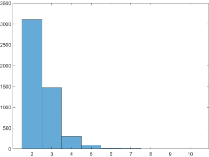
Figure 4: Histogram of $\tau$ in $11$-dimensional pump model.

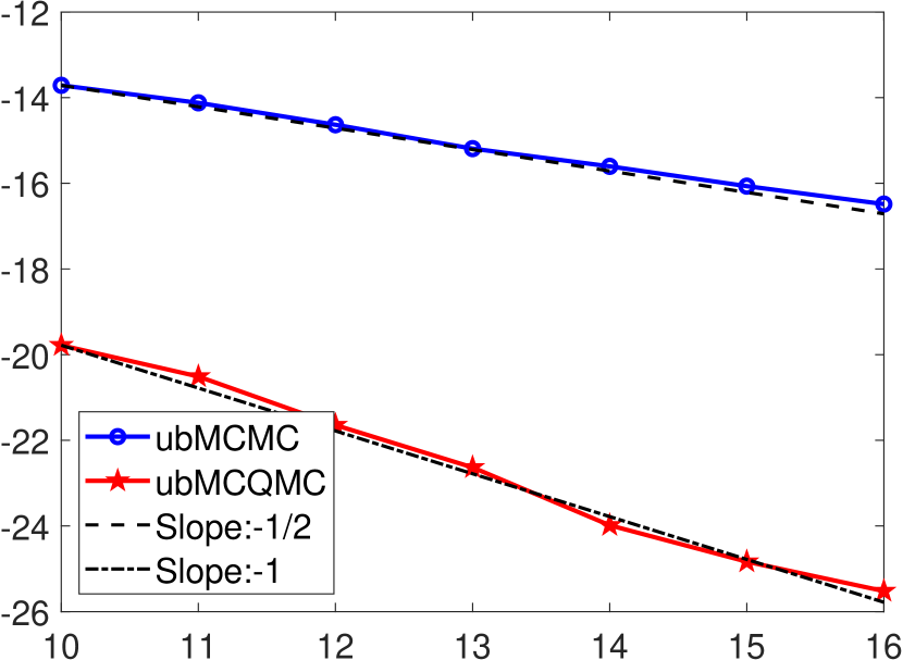
(a) $E[\lambda_{1}]$.

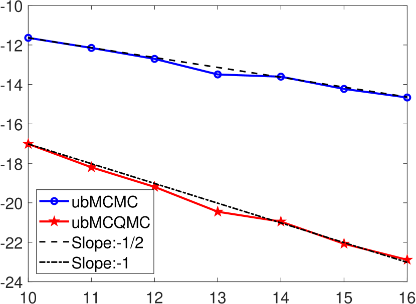
(b) $E[\lambda_{2}]$.

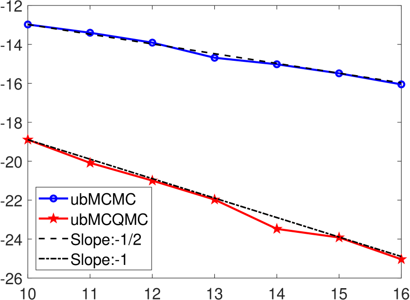
(c) $E[\lambda_{3}]$.

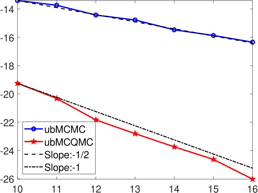
(d) $E[\lambda_{4}]$.

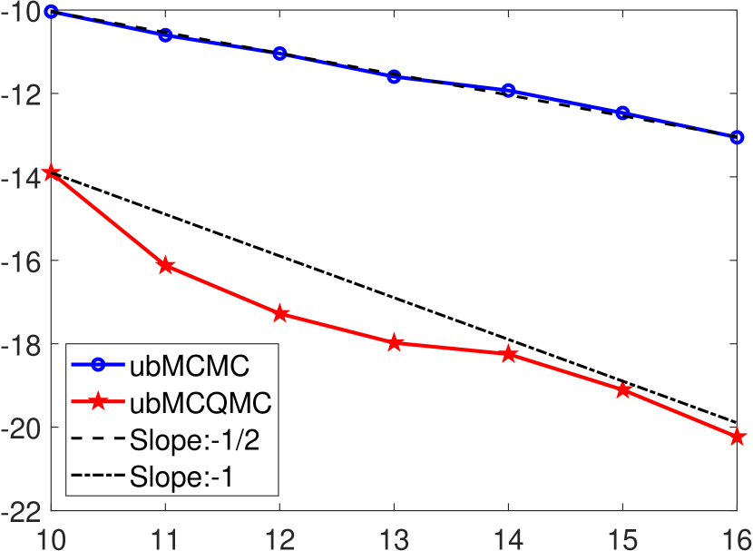
(e) $E[\lambda_{5}]$.

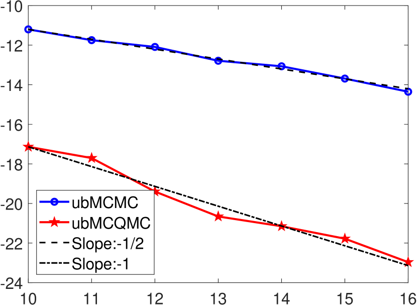
(f) $E[\lambda_{6}]$.

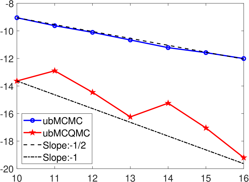
(g) $E[\lambda_{7}]$.

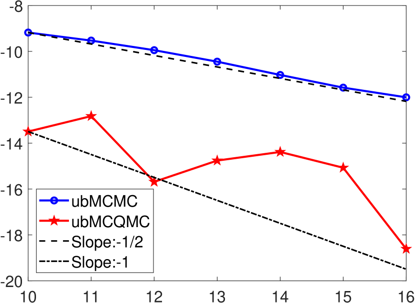
(h) $E[\lambda_{8}]$.

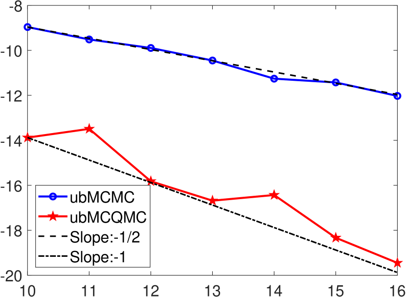
(i) $E[\lambda_{9}]$.

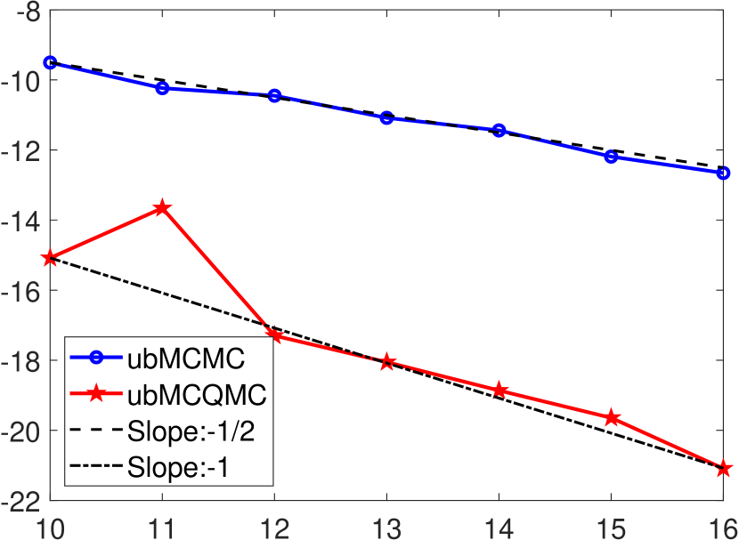
(j) $E[\lambda_{10}]$.

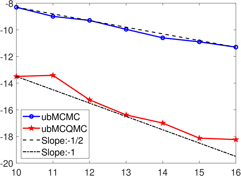
(k) $E[\beta]$.

Figure 5: RMSEs (on a $\log_{2}$ scale) of ubMCMC and ubMCQMC for estimating $E[\lambda_{j}],j=1,2,\ldots,10$ and $E[\beta]$.

Then, we take small samples $N$ for estimating $E[\beta]$ to compare the efficiency of $F_{k:m}(\bm{X},\bm{Y})$ in unbiased MCMC and unbiased MCQMC and that of MCMC estimators. Following the setting in the normal Gibbs model, for different choices of $k$ and $m$, over $1000$ independent experiments, the expected cost, the variance of estimators, and the loss of efficiency of unbiased MCMC and unbiased MCQMC are presented in Table 4. It can be seen that when $k=7,m=70$, i.e., $N=64$, the efficiency of unbiased MCMC is on par with that of standard MCMC methods. However, for unbiased MCQMC, achieving comparable efficiency to standard MCMC methods requires only $k=7,m=11$, i.e., $N=5$, resulting in a savings of sample size by a factor of $64/5\approx 13$.

Table 4: Cost, variance and the loss of efficiency for unbiased MCMC and unbiased MCQMC estimating $E[\beta]$.

$E[\beta]$	$k$	$m$	Cost	Variance	Inefficiency/$V_{\infty}$
ubMCMC	7	14	15.46	1.12E-04	1.7657 [t]
	7	35	36.46	3.44E-05	1.2744
	7	70	71.46	1.45E-05	1.0517 [b]
ubMCQMC	7	10	11.54	9.92E-05	1.1622 [t]
	7	11	12.54	8.17E-05	1.0403
	7	12	13.54	5.95E-05	0.8187 [b]

5.2 Probit regression model

Next we consider a $42$-dimensional model that was used in [40] to demonstrate the performance of unbiased MCQMC method in high-dimension. The model is a probit regression problem proposed in [10]. We follow the model setting in [40]. For $i=1,2,\ldots,39$, the response variable $y_{i}$ is a binary variable, taking values of $0$ or $1$. If the subject exhibits vascular constriction, then $y_{i}$ takes the value 1; otherwise, it is 0. The predictor variables are represented as $(v_{i},r_{i})$, where $v_{i}$ represents the volume of inspired air, and $r_{i}$ represents the rate of inspired air. The probit model is expressed as $y_{i}=1_{z_{i}>0}$ with $z_{i}=\beta_{0}+\beta_{1}v_{i}+\beta_{2}r_{i}+\epsilon_{i}$, where $\epsilon_{i}\sim\mathcal{N}(0,1)$, and $\{\epsilon_{i}\}_{i=1}^{39}$ are mutually independent. Thus, given $(v_{1},r_{1}),(v_{2},r_{2}),\ldots,(v_{39},r_{39})$, $z_{i}\sim\mathcal{N}(\beta_{0}+\beta_{1}v_{i}+\beta_{2}r_{i},1)$, and $\{z_{i}\}_{i=1}^{39}$ are mutually independent. Let $\beta=(\beta_{0},\beta_{1},\beta_{2})^{T}$, $Z=(z_{1},z_{2},\ldots,z_{39})^{T}$, and $X$ is a $39\times 3$ matrix with the $i$-th row being $(1,v_{i},r_{i})$. Our goal is to estimate the posterior mean $E[\beta]$. Taking a non-informative prior for $\beta$, we have

$$\beta|z_{1},z_{2},\ldots,z_{39} \sim\mathcal{N}\left(\left(X^{T}X\right)^{-1}X^{T}Z,\left(X^{T}X\right)^{-1}\right),$$

$$z_{i}|\beta,z_{j},j\neq i \sim\begin{cases}N\left(\beta_{0}+\beta_{1}v_{i}+\beta_{2}r_{i},1\right)\text{~{}turncated to~{}}[0,\infty),\text{~{}if~{}}y_{i}=1,\\ N\left(\beta_{0}+\beta_{1}v_{i}+\beta_{2}r_{i},1\right)\text{~{}turncated to~{}}(-\infty,0],\text{~{}if~{}}y_{i}=0.\end{cases}$$

Suppose that the random variable $Q_{2}$ follows the truncated distribution of cumulative distribution function $H$ over the interval $(a,b)$, then $Q_{2}=H^{-1}(H(a)+(H(b)-H(a))u),u\sim U(0,1)$ [34]. The specific form of the update function is clear. After $5000$ simulations, we get the histogram of $\tau$ in Figure 6. We find that the $99.9\%$ quantile of $\tau$ is $60.5$. We chose $k=61$. For $R=100$, we consider $m-k+1=N\in\{2^{10},2^{11},\ldots,2^{16}\}$. Figure 7 shows the RMSEs of ubMCMC and ubMCQMC for estimating $E[\beta]$ on a $\log_{2}$ scale. It can be observed that the red lines are positioned between the lines with slopes of $-1/2$ and $-1$. Thus, for this 42-dimensional model, the convergence rate of unbiased MCQMC may fall between $O(N^{-1/2})$ and $O(N^{-1})$. Comparing to the nearly $O(N^{-1})$ convergence rate of unbiased MCQMC observed in the $11$-dimensional pump model and the $3$-dimensional Gibbs model, we believe that the convergence rate of unbiased MCQMC may suffer from the curse of dimensionality, similar to that of plain QMC.

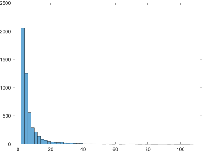
Figure 6: Histogram of $\tau$ in 42-dimensional probit model.

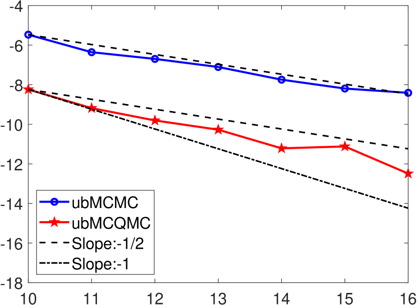
(a) $E[\beta_{1}]$

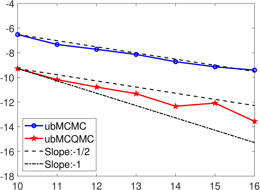
(b) $E[\beta_{2}]$

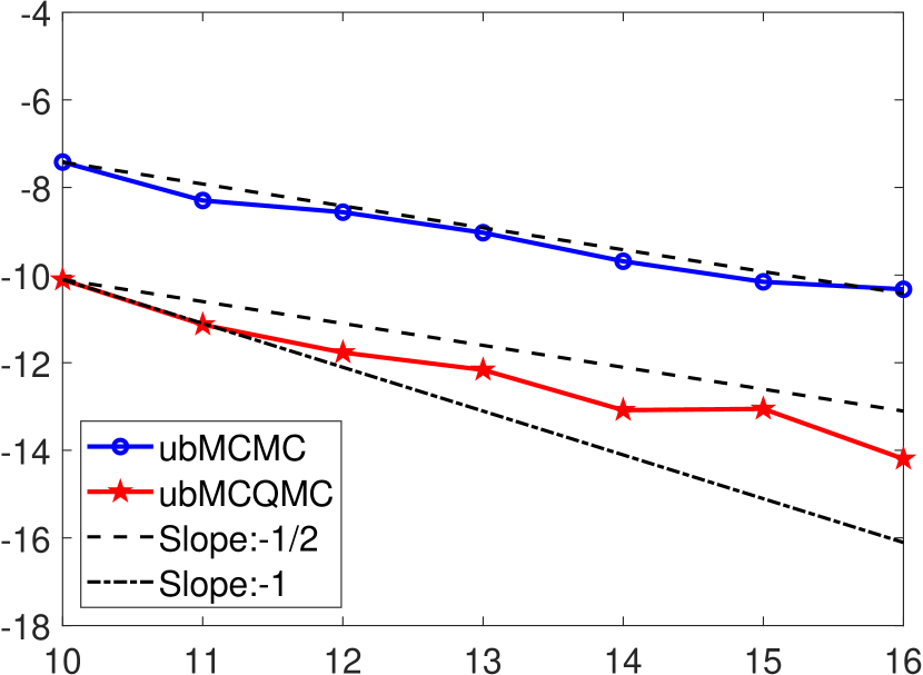
(c) $E[\beta_{3}]$

Figure 7: RMSEs (on a $\log_{2}$ scale) of ubMCMC and ubMCQMC for estimating $E[\beta_{i}],i=1,2,3$.

Figure 8 presents $\log_{2}$-RMSEs for estimating posterior mean of the latent variables $z_{1},z_{2},\ldots,z_{39}$ for $N=2^{16}$. The vertical axis represents $\log_{2}(\sqrt{\hat{\sigma}^{2}})$, and the number of the horizontal axis indicates the subscript of latent variables. Similar curves are observed for other sample sizes. It can be seen that unbiased MCQMC also leads to large variance reduction.

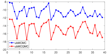
Figure 8: RMSEs (on a $\log_{2}$ scale) of ubMCMC and ubMCQMC for estimating $E[z_{i}],i=1,2,\ldots,39$ with $N=2^{16}$.

Then, we also take small samples $N$ for estimating $E[\beta_{1}]$ to compare the efficiency of $F_{k:m}(\bm{X},\bm{Y})$ and that of MCMC estimators. Following the setting in normal Gibbs model, for different choice of $k$ and $m$, over $1000$ independent experiments, the expected cost, the variance of estimators, and the loss of efficiency of unbiased MCMC and unbiased MCQMC are presented in Table 5. We observe that when $k=61,m=610$, i.e., $N=550$, the efficiency of unbiased MCMC is comparable to that of standard MCMC methods. However, for unbiased MCQMC, we just require $k=61,m=85$, i.e., $N=25$ to achieve efficiency comparable to standard MCMC methods, saving a sample size of $550/25=22$ times.

Table 5: Cost, variance and the loss of efficiency for unbiased MCMC and unbiased MCQMC estimating $E[\beta_{1}]$.

$E[\beta_{1}]$	$k$	$m$	Cost	Variance	Inefficiency/$V_{\infty}$
ubMCMC	61	122	127.25	6.29E-04	1.7879 [t]
	61	305	310.25	1.84E-04	1.2776
	61	610	615.25	7.96E-05	1.0938 [b]
ubMCQMC	61	80	86.13	8.69E-04	1.6717 [t]
	61	85	91.12	5.29E-04	1.0766
	61	90	96.12	3.97E-04	0.8526 [b]

6 Conclusions

By incorporating array-(W)CUD sequences into the first-step sampling of the maximal coupling method in unbiased MCMC, we propose unbiased MCQMC method for Gibss sampler. This method maintains the unbiasedness of the estimator and successfully accelerates the convergence rate of unbiased MCMC. We suggest that utilizing array-(W)CUD sequences after a significant quantile of the meeting time to improve the performance of unbiased MCQMC. Moreover, without relying on Markov property and the geometric drift condition, which were required in [20], we provide a simpler proof for the upper bound of the second moment of the bias term. Based on this, we attribute the convergence rate problem of unbiased MCQMC to the convergence rate challenge of MCQMC. Enhancing the convergence rate theory for MCQMC would also contribute to addressing the convergence rate theory for unbiased MCQMC. Through a series of comprehensive experiments, unbiased MCQMC has shown significant improvement in variance reduction compared to unbiased MCMC. Especially in low dimensional cases, compared to the $O(N^{-1/2})$ convergence rate of unbiased MCMC, unbiased MCQMC achieves an almost $O(N^{-1})$ convergence rate. In high dimensional cases, unbiased MCQMC may suffer form the curse of dimensionality, similar to that of QMC. However, QMC has been successfully applied to solve high-dimensional financial problems [15, 16, 41]. To leverage the performance of QMC, it is often necessary to use dimension reduction techniques [1, 18, 26, 43] on high dimensional objective functions. In our future work, we aim to develop useful dimension reduction techniques for unbiased MCQMC to further enhance its efficiency. Moreover, when parallel resources are limited, thanks to the $O(N^{-1+\epsilon})$ convergence rate in unbiased MCQMC, running longer chains instead of repeating more chains can achieve higher precision for a fixed budget. On the other hand, in the setting of parallelization, unbiased MCQMC can save several times the sample size to achieve the similar efficiency of unbiased MCMC. Noting that we focus on Gibbs samplers in this work. In fact, the unbiased MCQMC method can also be applied to the M-H algorithm, but its performance is not as pronounced as in Gibbs samplers. This is because the acceptance-rejection proposal step affects the uniformity of the array-(W)CUD sequence [40]. Improving the unbiased MCQMC method to make it more effective in the M-H algorithm is also a direct of our future work.

Appendix A Proof of Proposition 2

To prove Proposition 2, we require a useful lemma as follows.

Lemma A.1.

Under Assumptions 1-3, for all $k\geq 0$ and sample size $N>0$, let $m=N+k-1$, then we have

$$E\left[\left(\sum_{l=k+1}^{\infty}\frac{l-k}{m-k+1}\left|f(X_{l})-f(Y_{l-1})\right|\right)^{2}\right]\leq\tilde{C}\left(\frac{\tilde{\delta}^{k+1}}{N(1-\tilde{\delta})^{2}}\right)^{2},$$ (14)

and

$$E\left[\left(\sum_{l=k+1}^{\infty}\left|f(X_{l})-f(Y_{l-1})\right|\right)^{2}\right]\leq\tilde{C}\left(\frac{\tilde{\delta}^{k+1}}{1-\tilde{\delta}}\right)^{2}.$$ (15)

where $\tilde{C}=2(CD)^{\frac{2}{2+\eta}}$, $\tilde{\delta}=\delta^{\frac{\eta}{4+2\eta}}$ with $D$ and $\eta$ defined in Assumption 1 and $C$ and $\delta$ defined in Assumption 2.

Proof.

Denote $X^{\prime}_{t}=X_{t+k-1},Y^{\prime}_{t}=Y_{t+k-1},\Delta^{\prime}_{t}=f(X^{\prime}_{t+1})-f(Y^{\prime}_{t}),t\geq 1$. We have

$$\sum_{l=k+1}^{\infty}\frac{l-k}{m-k+1}\left|f(X_{l})-f(Y_{l-1})\right| =\sum_{h=1}^{\infty}\frac{h}{N}\left|f(X_{h+k})-f(Y_{h+k-1})\right|$$

$$=\sum_{h=1}^{\infty}\frac{h}{N}\left|f(X^{\prime}_{h+1})-f(Y^{\prime}_{h})\right|$$

$$=\sum_{h=1}^{\infty}\frac{h}{N}\left|\Delta^{\prime}_{h}1_{\{\tau>h+k\}}\right|,$$

where $1_{\{\tau>h+k\}}$ is a indicative function. Note that $\Delta^{\prime}_{h}=0$ if $h\geq\tau-k$ by Assumption 3. Then, it follows that

$$E\left[\left(\sum_{h=1}^{\infty}\frac{h}{N}\left|\Delta^{\prime}_{h}1_{\{\tau>h+k\}}\right|\right)^{2}\right] =\frac{1}{N^{2}}\sum_{i=1}^{\infty}\sum_{j=1}^{\infty}ijE\left[\left|\Delta^{\prime}_{i}1_{\{\tau>i+k\}}\right|\cdot\left|\Delta^{\prime}_{j}1_{\{\tau>j+k\}}\right|\right].$$

By Cauchy-Schwarz inequality, we have

$$E\left[\left|\Delta^{\prime}_{i}1_{\{\tau>i+k\}}\right|\cdot\left|\Delta^{\prime}_{j}1_{\{\tau>j+k\}}\right|\right] \leq\left(E\left[\left|\Delta^{\prime}_{i}1_{\{\tau>i+k\}}\right|^{2}\right]E\left[\left|\Delta^{\prime}_{j}1_{\{\tau>j+k\}}\right|^{2}\right]\right)^{1/2}$$

$$=\left(E\left[\left|\Delta^{\prime}_{i}\right|^{2}1_{\{\tau>i+k\}}\right]E\left[\left|\Delta^{\prime}_{j}\right|^{2}1_{\{\tau>j+k\}}\right]\right)^{1/2}.$$

For any $i\geq 1$, by Holder inequailty with $p=1+\eta/2$, for any $\eta>0$, we see that

$$E\left[\left|\Delta^{\prime}_{i}\right|^{2}1_{\{\tau>i+k\}}\right] \leq E\left[\left|\Delta^{\prime}_{i}\right|^{2+\eta}\right]^{\frac{2}{2+\eta}}E\left[1\{\tau>i+k\}^{\frac{2+\eta}{\eta}}\right]^{\frac{\eta}{2+\eta}}$$

$$\leq E\left[\left|\Delta^{\prime}_{i}\right|^{2+\eta}\right]^{\frac{2}{2+\eta}}E\left[1\{\tau>i+k\}\right]^{\frac{\eta}{2+\eta}}.$$

By Assumption 2, we have

$$E\left[1\{\tau>i+k\}\right]^{\frac{\eta}{2+\eta}}=\mathbb{P}(\tau>i+k)^{\frac{\eta}{2+\eta}}\leq(C\delta^{i+k})^{\frac{\eta}{2+\eta}}=C^{\frac{\eta}{2+\eta}}\tilde{\delta}^{2(k+i)},$$

where $\tilde{\delta}=\delta^{\frac{\eta}{4+2\eta}}$. Then, by Minkowski inequailty and Assumption 1, we obtain

$$E\left[\left|\Delta^{\prime}_{i}\right|^{2+\eta}\right]^{\frac{2}{2+\eta}} =E[\left|f(X^{\prime}_{i+1})-f(Y^{\prime}_{i})\right|^{2+\eta}]^{\frac{2}{2+\eta}}$$

$$=E\left[\left|f(X_{i+k})-f(Y_{i+k-1})\right|^{2+\eta}\right]^{\frac{2}{2+\eta}}$$

$$\leq E\left[\left|f(X_{i+k})\right|^{2+\eta}\right]^{\frac{2}{2+\eta}}+E\left[\left|-f(Y_{i+k-1})\right|^{2+\eta}\right]^{\frac{2}{2+\eta}}$$

$$=E\left[\left|f(X_{i+k})\right|^{2+\eta}\right]^{\frac{2}{2+\eta}}+E\left[\left|f(X_{i+k-1})\right|^{2+\eta}\right]^{\frac{2}{2+\eta}}\leq 2D^{\frac{\eta}{2+\eta}}.$$

In the last equality, we have used the fact that for any $t\geq 0$, $X_{t}$ and $Y_{t}$ share the same distribution. Then, it follows that for any $i\geq 1$,

$$E\left[\left|\Delta^{\prime}_{i}\right|^{2}1_{\{\tau>i+k\}}\right]\leq 2D^{\frac{\eta}{2+\eta}}C^{\frac{\eta}{2+\eta}}\tilde{\delta}^{2(k+i)}\leq\tilde{C}\tilde{\delta}^{2(k+i)},$$

where $\tilde{C}=2(CD)^{\frac{\eta}{2+\eta}}$.

Hence, it follows that

$$E\left[\left(\sum_{l=k+1}^{\infty}\frac{l-k}{m-k+1}\{f(X_{l})-f(Y_{l-1})\}\right)^{2}\right]$$

$$= \frac{1}{N^{2}}\sum_{i=1}^{\infty}\sum_{j=1}^{\infty}ijE\left[\left|\Delta^{\prime}_{i}1_{\{\tau>i+k\}}\right|\left|\Delta^{\prime}_{j}1_{\{\tau>j+k\}}\right|\right]$$

$$\leq \frac{1}{N^{2}}\sum_{i=1}^{\infty}\sum_{j=1}^{\infty}ij\left(E\left[\left|\Delta^{\prime}_{i}\right|^{2}1_{\{\tau>i+k\}}\right]E\left[\left|\Delta^{\prime}_{j}\right|^{2}1_{\{\tau>j+k\}}\right]\right)^{1/2}$$

$$\leq \frac{1}{N^{2}}\sum_{i=1}^{\infty}\sum_{j=1}^{\infty}ij\left(\tilde{C}^{2}\tilde{\delta}^{2(k+i)}\tilde{\delta}^{2(k+j)}\right)^{1/2}$$

$$\leq \frac{\tilde{C}\tilde{\delta}^{2k}}{N^{2}}\sum_{i=1}^{\infty}i\tilde{\delta}^{i}\sum_{j=1}^{\infty}j\tilde{\delta}^{j}=\frac{\tilde{C}\tilde{\delta}^{2k}}{N^{2}}\left(\frac{\tilde{\delta}}{(1-\tilde{\delta})^{2}}\right)^{2}=\tilde{C}\left(\frac{\tilde{\delta}^{k+1}}{N(1-\tilde{\delta})^{2}}\right)^{2}.$$

Here we use the fact that $\sum_{i=1}^{\infty}i\tilde{\delta}^{i}=\frac{\tilde{\delta}}{1-\tilde{\delta}}\sum_{i=1}^{\infty}i\tilde{\delta}^{i-1}(1-\tilde{\delta})=\frac{\tilde{\delta}}{(1-\tilde{\delta})^{2}}.$ Similarly, we obtain

$$E\left[\left(\sum_{l=k+1}^{\infty}\left|f(X_{l})-f(Y_{l-1})\right|\right)^{2}\right]$$

$$= \sum_{i=1}^{\infty}\sum_{j=1}^{\infty}E\left[\left|\Delta^{\prime}_{i}1_{\{\tau>i+k\}}\right|\left|\Delta^{\prime}_{j}1_{\{\tau>j+k\}}\right|\right]$$

$$\leq \sum_{i=1}^{\infty}\sum_{j=1}^{\infty}\left(E\left[\left|\Delta^{\prime}_{i}\right|^{2}1_{\{\tau>i+k\}}\right]E\left[\left|\Delta^{\prime}_{j}\right|^{2}1_{\{\tau>j+k\}}\right]\right)^{1/2}$$

$$\leq \sum_{i=1}^{\infty}\sum_{j=1}^{\infty}\left(\tilde{C}^{2}\tilde{\delta}^{2(k+i)}\tilde{\delta}^{2(k+j)}\right)^{1/2}$$

$$\leq \tilde{C}\tilde{\delta}^{2k}\sum_{i=1}^{\infty}\tilde{\delta}^{i}\sum_{j=1}^{\infty}\tilde{\delta}^{j}=\tilde{C}\tilde{\delta}^{2k}\left(\frac{\tilde{\delta}}{1-\tilde{\delta}}\right)^{2}=\tilde{C}\left(\frac{\tilde{\delta}^{k+1}}{1-\tilde{\delta}}\right)^{2}.$$

This completes the proof. ∎

Now we are ready to prove Proposition 2.

Proof of Proposition 2.

By $F_{k:m}(\bm{X},\bm{Y})$ defined in (7), we know that

$$\text{BC}_{k:m}^{2} =\sum_{l=k+1}^{\tau-1}\min\left(1,\frac{l-k}{m-k+1}\right)\{f(X_{l})-f(Y_{l-1})\}$$

$$:=\begin{cases}\@slowromancap i@,\text{~{}if~{}}\tau\leq m+1,\\ \@slowromancap ii@_{1}+\@slowromancap ii@_{2},\text{~{}if~{}}\tau>m+1,\\ \end{cases}$$

where

$$\@slowromancap i@ =\sum\limits_{l=k+1}^{\tau-1}\frac{l-k}{m-k+1}\{f(X_{l})-f(Y_{l-1})\},$$

$$\@slowromancap ii@_{1} =\sum\limits_{l=k+1}^{m}\frac{l-k}{m-k+1}\{f(X_{l})-f(Y_{l-1})\},$$

$$\@slowromancap ii@_{2} =\sum\limits_{l=m+1}^{\tau-1}\{f(X_{l})-f(Y_{l-1})\}.$$

By the law of total expectation, it follows that

$$E\left[\text{BC}_{k:m}^{2}\right] =E\left[\text{BC}_{k:m}^{2}|\tau\leq m+1\right]P(\tau\leq m+1)$$ (16)

$$+E\left[\text{BC}_{k:m}^{2}|\tau>m+1\right]P(\tau>m+1)$$

$$=E\left[\@slowromancap i@^{2}|\tau\leq m+1\right]P(\tau\leq m+1)$$

$$+E\left[\left(\@slowromancap ii@_{1}+\@slowromancap ii@_{2}\right)^{2}|\tau>m+1\right]P(\tau>m+1).$$

For the first term of (16), we see that

$$E\left[\@slowromancap i@^{2}|\tau\leq m+1\right]P(\tau\leq m+1)=E\left[\@slowromancap i@^{2}1_{\{\tau\leq m+1\}}\right]\leq E\left[\@slowromancap i@^{2}\right].$$

Denote $X^{\prime}_{t}=X_{t+k-1},Y^{\prime}_{t}=Y_{t+k-1},\Delta^{\prime}_{t}=f(X^{\prime}_{t+1})-f(Y^{\prime}_{t}),t\geq 1$. It then follows that

$$|\@slowromancap i@| =\left|\sum_{l=k+1}^{\tau-1}\frac{l-k}{m-k+1}\{f(X_{l})-f(Y_{l-1})\}\right|$$

$$\leq\sum_{l=k+1}^{\tau-1}\frac{l-k}{m-k+1}\left|f(X_{l})-f(Y_{l-1})\right|$$

$$=\sum_{l=k+1}^{\infty}\frac{l-k}{m-k+1}\left|f(X_{l})-f(Y_{l-1})\right|.$$

By Lemma A.1, we have

$$E\left[\@slowromancap i@^{2}\right]\leq E\left[\left(\sum_{l=k+1}^{\infty}\frac{l-k}{m-k+1}\left|f(X_{l})-f(Y_{l-1})\right|\right)^{2}\right]\leq\tilde{C}\left(\frac{\tilde{\delta}^{k+1}}{N(1-\tilde{\delta})^{2}}\right)^{2}.$$

Hence,

$$E\left[\@slowromancap i@^{2}|\tau\leq m+1\right]P(\tau\leq m+1)\leq E\left[\@slowromancap i@^{2}\right]\leq\tilde{C}\left(\frac{\tilde{\delta}^{k+1}}{N(1-\tilde{\delta})^{2}}\right)^{2}.$$ (17)

For the second term of (16), we also have

$$E\left[\left.\left(\@slowromancap ii@_{1}+\@slowromancap ii@_{2}\right)^{2}\right|\tau>m+1\right]P(\tau>m+1)$$

$$\leq E\left[\left(\@slowromancap ii@_{1}+\@slowromancap ii@_{2}\right)^{2}\right]\leq 2\left(E\left[\@slowromancap ii@_{1}^{2}\right]+E\left[\@slowromancap ii@_{2}^{2}\right]\right).$$

Similarly, by (14) and (15), we find that

$$E\left[\@slowromancap ii@_{1}^{2}\right] =E\left[\left|\sum_{l=k+1}^{m}\frac{l-k}{m-k+1}\{f(X_{l})-f(Y_{l-1})\}\right|^{2}\right]$$

$$\leq E\left[\left(\sum_{l=k+1}^{\infty}\frac{l-k}{m-k+1}\left|f(X_{l})-f(Y_{l-1})\right|\right)^{2}\right]\leq\tilde{C}\left(\frac{\tilde{\delta}^{k+1}}{N(1-\tilde{\delta})^{2}}\right)^{2},$$

and

$$E\left[\@slowromancap ii@_{2}^{2}\right] =E\left[\left|\sum_{l=m+1}^{\tau-1}\{f(X_{l})-f(Y_{l-1})\}\right|^{2}\right]$$

$$\leq E\left[\left(\sum_{l=m+1}^{\infty}\left|f(X_{l})-f(Y_{l-1})\right|\right)^{2}\right]\leq\tilde{C}\left(\frac{\tilde{\delta}^{m+1}}{1-\tilde{\delta}}\right)^{2}.$$

Note that

$$\frac{\tilde{C}\left(\frac{\tilde{\delta}^{m+1}}{1-\tilde{\delta}}\right)^{2}}{\tilde{C}\left(\frac{\tilde{\delta}^{k+1}}{N(1-\tilde{\delta})^{2}}\right)^{2}}=\left(N\tilde{\delta}^{m-k}(1-\tilde{\delta})\right)^{2}=\left(N\tilde{\delta}^{N}\frac{1-\tilde{\delta}}{\tilde{\delta}}\right)^{2},$$

that is

$$E\left[\@slowromancap ii@_{2}^{2}\right]\leq\left(N\tilde{\delta}^{N}\frac{1-\tilde{\delta}}{\tilde{\delta}}\right)^{2}\tilde{C}\left(\frac{\tilde{\delta}^{k+1}}{N(1-\tilde{\delta})^{2}}\right)^{2}.$$

Hence, it follows that

$$E\left[\@slowromancap ii@_{1}^{2}\right]+E\left[\@slowromancap ii@_{2}^{2}\right]\leq \tilde{C}\left(1+\left(N\tilde{\delta}^{N}\frac{1-\tilde{\delta}}{\tilde{\delta}}\right)^{2}\right)\left(\frac{\tilde{\delta}^{k+1}}{N(1-\tilde{\delta})^{2}}\right)^{2}.$$ (18)

Therefore, by (16) and (17) together with (18), we have

$$E\left[\text{BC}_{k:m}^{2}\right] \leq\tilde{C}\left(\frac{\tilde{\delta}^{k+1}}{N(1-\tilde{\delta})^{2}}\right)^{2}+2\tilde{C}\left(1+\left(N\tilde{\delta}^{N}\frac{1-\tilde{\delta}}{\tilde{\delta}}\right)^{2}\right)\left(\frac{\tilde{\delta}^{k+1}}{N(1-\tilde{\delta})^{2}}\right)^{2}$$

$$=\left(3+2\left(N\tilde{\delta}^{N}\frac{1-\tilde{\delta}}{\tilde{\delta}}\right)^{2}\right)\tilde{C}\left(\frac{\tilde{\delta}^{k+1}}{N(1-\tilde{\delta})^{2}}\right)^{2}\leq C_{\delta}\frac{\tilde{\delta}^{2k}}{\left(N^{2}\right)},$$

where

$$C_{\delta}=\tilde{C}\dfrac{3+2\left(\left(-\frac{\tilde{\delta}^{-1/\ln(\tilde{\delta})}}{\ln(\tilde{\delta})}\right)\frac{1-\tilde{\delta}}{\tilde{\delta}}\right)^{2}}{\left(\frac{(1-\tilde{\delta})^{2}}{\tilde{\delta}}\right)^{2}}.$$

In the last inequality, we have used the fact that the function $x\tilde{\delta}^{x}$ reaches its maximum at $-1/\ln(\tilde{\delta})$. This completes the proof. ∎

References

- [1] Peter A Acworth, Mark Broadie, and Paul Glasserman. A comparison of some Monte Carlo and quasi-Monte Carlo techniques for option pricing. In Monte Carlo and Quasi-Monte Carlo Methods 1996, pages 1–18. Springer, 1998.
- [2] Su Chen. Consistency and convergence rate of Markov chain quasi Monte Carlo with examples. PhD thesis, Stanford University, 2011.
- [3] Su Chen, Josef Dick, and Art B Owen. Consistency of Markov chain quasi-Monte Carlo on continuous state spaces. The Annals of Statistics, 39(2):673–701, 2011.
- [4] Su Chen, Makoto Matsumoto, Takuji Nishimura, and Art B. Owen. New inputs and Methods for Markov chain quasi-Monte Carlo. In Monte Carlo and Quasi-Monte Carlo Methods 2010, volume 23, pages 313–327. Springer Berlin Heidelberg, 2012.
- [5] Roy Cranley and Thomas NL Patterson. Randomization of number theoretic methods for multiple integration. SIAM Journal on Numerical Analysis, 13(6):904–914, 1976.
- [6] Luc Devroye. Non-uniform Random Variate Generation. Springer, 1986.
- [7] Josef Dick and Friedrich Pillichshammer. Digital Nets and Sequences: Discrepancy Theory and Quasi-Monte Carlo Integration. Cambridge University Press, 2010.
- [8] Josef Dick and Daniel Rudolf. Discrepancy estimates for variance bounding Markov chain quasi-Monte Carlo. Electronic Journal of Probability, 19:1–24, 2014.
- [9] Josef Dick, Daniel Rudolf, and Houying Zhu. Discrepancy bounds for uniformly ergodic Markov chain quasi-Monte Carlo. The Annals of Applied Probability, 26(5):3178–3205, 2016.
- [10] D. J. Finney. The estimation from individual records of the relationship between dose and quantal response. Biometrika, 34(320–334), 1947.
- [11] Paul Glasserman. Monte Carlo Methods in Financial Engineering, volume 53. Springer, 2004.
- [12] Peter W Glynn and Chang-han Rhee. Exact estimation for Markov chain equilibrium expectations. Journal of Applied Probability, 51(A):377–389, 2014.
- [13] Shin Harase. A table of short-period Tausworthe generators for Markov chain quasi-Monte Carlo. Journal of Computational and Applied Mathematics, 384:113136, 2021.
- [14] Shin Harase. A search for short-period Tausworthe generators over with application to Markov chain quasi-Monte Carlo. Journal of Statistical Computation and Simulation, pages 1–23, 2024.
- [15] Zhijian He and Xiaoqun Wang. Good path generation methods in quasi-Monte Carlo for pricing financial derivatives. SIAM Journal on Scientific Computing, 36(2):B171–B179, 2014.
- [16] Zhijian He and Xiaoqun Wang. An integrated quasi-Monte Carlo method for handling high dimensional problems with discontinuities in financial engineering. Computational Economics, 57(2):693–718, 2021.
- [17] Zhijian He, Zhan Zheng, and Xiaoqun Wang. On the error rate of importance sampling with randomized quasi-Monte Carlo. SIAM Journal on Numerical Analysis, 61(2):515–538, 2023.
- [18] Junichi Imai and Ken Seng Tan. A general dimension reduction technique for derivative pricing. Journal of Computational Finance, 10(2):129–155, 2006.
- [19] Pierre E Jacob, Fredrik Lindsten, and Thomas B Schön. Smoothing with couplings of conditional particle filters. Journal of the American Statistical Association, 115(530):721–729, 2020.
- [20] Pierre E. Jacob, John O’Leary, and Yves F. Atchadé. Unbiased Markov chain Monte Carlo methods with couplings. Journal of the Royal Statistical Society Series B: Statistical Methodology, 82(3):543–600, 2020.
- [21] J. G. Liao. Variance reduction in Gibbs Sampler using quasi random numbers. Journal of Computational and Graphical Statistics, 7(3):253–266, 1998.
- [22] Sifan Liu. Langevin quasi-Monte Carlo. arXiv preprint arXiv:2309.12664, 2023.
- [23] Pierre L’Ecuyer. Quasi-Monte Carlo methods with applications in finance. Finance and Stochastics, 13:307–349, 2009.
- [24] Charles C Margossian, Matthew D Hoffman, Pavel Sountsov, Lionel Riou-Durand, Aki Vehtari, and Andrew Gelman. Nested : Assessing the convergence of Markov chains Monte Carlo when running many short chains. arXiv preprint arXiv:2110.13017, 2022.
- [25] Lawrence Middleton, George Deligiannidis, Arnaud Doucet, and Pierre E. Jacob. Unbiased Markov chain Monte Carlo for intractable target distributions. Electronic Journal of Statistics, 14(2):2842–2891, 2020.
- [26] Bradley Moskowitz and Russel E Caflisch. Smoothness and dimension reduction in quasi-Monte Carlo methods. Mathematical and Computer Modelling, 23(8):37–54, 1996.
- [27] Radford M Neal. Circularly-coupled Markov chain sampling. arXiv preprint arXiv:1711.04399, 2017.
- [28] Geoff K Nicholls, Colin Fox, and Alexis Muir Watt. Coupled MCMC with a randomized acceptance probability. arXiv preprint arXiv:1205.6857, 2012.
- [29] Harald Niederreiter. Pseudo-random numbers and optimal coefficients. Advances in Mathematics, 26, 1977.
- [30] Harald Niederreiter. Multidimensional numerical integration using pseudorandom numbers. Mathematical Programming Study, 27:17–38, 1986.
- [31] Harald Niederreiter. Random Number Generation and Quasi-Monte Carlo Methods. Society for Industrial and Applied Mathematics, 1992.
- [32] Art B Owen. Randomly permuted -nets and -sequences. In Monte Carlo and Quasi-Monte Carlo Methods in Scientific Computing, pages 299–317. Springer, 1995.
- [33] Art B Owen. Multidimensional variation for quasi-Monte Carlo. In Contemporary Multivariate Analysis And Design Of Experiments: In Celebration of Professor Kai-Tai Fang’s 65th Birthday, pages 49–74. World Scientific, 2005.
- [34] Art B. Owen. Monte Carlo Theory, Methods and Examples. https://artowen.su.domains/mc/, 2013.
- [35] Art B. Owen. Practical Quasi-Monte Carlo Integration. https://artowen.su.domains/mc/practicalqmc.pdf, 2023.
- [36] Art B. Owen and Seth D. Tribble. A quasi-Monte Carlo Metropolis algorithm. Proceedings of the National Academy of Sciences, 102(25):8844–8849, 2005.
- [37] Christian P Robert and George Casella. Monte Carlo Statistical Methods. Springer, 2nd edition, 2004.
- [38] I. M. Sobol’. The distribution of points in a cube and the accurate evaluation of integrals. USSR Computational Mathematics and Mathematical Physics, 7(4):86–112, 1967.
- [39] Seth D Tribble. Markov chain Monte Carlo algorithms using completely uniformly distributed driving sequences. PhD thesis, Stanford University, 2007.
- [40] Seth D. Tribble and Art B. Owen. Construction of weakly CUD sequences for MCMC sampling. Electronic Journal of Statistics, 2(634–660), 2008.
- [41] Xiaoqun Wang and Kai Tai Fang. The effective dimension and quasi-Monte Carlo integration. Journal of Complexity, 19(2):101–124, 2003.
- [42] Chengfeng Weng, Xiaoqun Wang, and Zhijian He. Efficient computation of option prices and Greeks by quasi–Monte Carlo method with smoothing and dimension reduction. SIAM Journal on Scientific Computing, 39(2):B298–B322, 2017.
- [43] Ye Xiao and Xiaoqun Wang. Enhancing quasi-Monte Carlo simulation by minimizing effective dimension for derivative pricing. Computational Economics, 54:343–366, 2019.