Conjugate operators for transparent, explorable
research outputs

Abstract.

Charts, figures, and text derived from data play an important role in decision making, from data-driven policy development to day-to-day choices informed by online articles. Making sense of, or fact-checking, outputs means understanding how they relate to the underlying data. Even for domain experts with access to the source code and data sets, this poses a significant challenge. In this paper we introduce a new program analysis framework which supports interactive exploration of fine-grained I/O relationships directly through computed outputs, making use of dynamic dependence graphs. Our main contribution is a novel notion in data provenance which we call related inputs, a relation of mutual relevance or “cognacy” which arises between inputs when they contribute to common features of the output. Queries of this form allow readers to ask questions like “What outputs use this data element, and what other data elements are used along with it?”. We show how Jonsson and Tarski’s concept of conjugate operators on Boolean algebras appropriately characterises the notion of cognacy in a dependence graph, and give a procedure for computing related inputs over such a graph.

To demonstrate the approach in practice, we present a functional programming language called [OurLanguage] which automatically enriches visual outputs with interactions supporting related inputs and similar fine-grained queries, and show how these can aid comprehension using realistic examples. We show how to obtain more informative, contextualised queries via projection operators which factor out data contributed by specific inputs or demand associated with specific outputs. We also show how to derive a related outputs operator, capturing a dual cognacy relation between output features whenever they compete for common input data. Composed with suitable projections, this recovers a prior approach to the problem of brushing and linking in data visualisation based on Galois connections and execution traces. As well as generalising and extending this prior work, the graphical approach presented in this paper performs better (computationally) on most examples and is significantly simpler to implement, and thus easier to deploy to other languages.

1. Introduction: Towards Transparent Research Outputs

Whether formulating a national policy or simply deciding what groceries to buy, we increasingly rely on the charts, figures and text created by scientists and journalists. Interpreting these visual and textual summaries is essential to making informed decisions. However, most of the artefacts we encounter are opaque: they are unable to reveal anything about how they relate to the data they were derived from. Whilst one could in principle try to use the source code and data sources to reverse engineer some of these relationships, this requires substantial expertise, as well as valuable time spent away from the “comprehension context” in which we encountered the output in question. These difficulties are only compounded when the information presented draws on multiple data sources, such as medical meta-analyses (DerSimonian and Laird, 1986), ensemble models in climate science (Murphy et al., 2004), or queries that span multiple database tables (Selinger et al., 1979). Even professional reviewers may lack the resources or inclination to embark on such an activity. Perhaps more often than we would like, we end up taking things on trust.

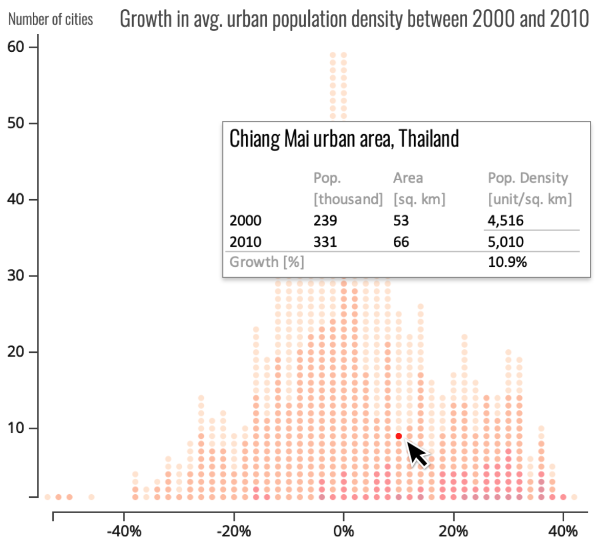
Figure 1. Hand-crafted data-transparent visualisation (Bremer and Ranzijn, 2015)

With traditional print media, a “disconnect” between outputs and underlying data is unavoidable. For digital media, other options are open to us. One way to improve things is to engineer visual artefacts to be more “self-explanatory” so they can reveal the relationship to the underlying data to an interested user. Consider the histogram in Figure 1 showing urban population growth in Asia over a 10-year period (Bremer and Ranzijn, 2015). There are many questions a reader might have about what this chart represents — in other words, how visual elements map to underlying data. Do the points represent individual cities? What does the colour scheme indicate? Which of the points represent large cities or small cities? Legends and other accompanying text can help, but some ambiguities inevitably remain. The entire value proposition of a summary after all is that it presents the big picture at the expense of certain detail.

Bremer and Ranzijn implemented an interactive feature that allow a user to explore some of these questions themselves in situ, i.e., directly from the chart. By selecting an individual point, they are able to bring up a view showing the data that point was calculated from. In this case the highlighted dot represents data for Chiang Mai and the plotted value of 10.9% was derived from an increase in population density from 4,416 to 5,010 people per sq. km.

1.1. Data transparency as PL infrastructure

Features like these are valuable comprehension aids but are laborious to implement by hand. They also require the author to anticipate the queries a user might have and do not readily generalise: for example Bremer and Ranzijn’s visualisation only allows the user to select one point at a time.

For these reasons, there has been recent interest in treating data transparency and exploration as a programming language infrastructure problem, baking dependency metadata directly into outputs so that interactive queries of this sort can be supported automatically. The author of the content no longer has to concern themselves with these tricky features, and the consumer of the content now has the best of both worlds: the ability to explore detail on an as-needed basis in the context of the high-level perspective offered by the visual summary. The relationship to data can be incrementally discoverable, revealed as the user interacts with the parts of the output they care about, ideally with some kind of formal guarantee that the revealed data is in some sense “minimal and sufficient”.

In data visualisation it has long been recognised that when users interact with visual elements by clicking or lassoing, the intention is typically to manipulate the underlying data; this has lead to various techniques for inverting selections in visual space to obtain selections in the input data space (North and Shneiderman, 2000; Heer et al., 2008). Psallidas and Wu (2018) were the first to propose techniques based on fine-grained data provenance; for a relational visualisation language, they describe how to “backward trace” from output selections to input selections, and then “forward trace” to find related output selections in other views, to support a popular feature called linked brushing. Perera et al. (2022) implemented a similar approach for a general-purpose functional language using a pair of dependency-tracking operators, written here as $\displaystyle\triangledown$ (demands) and $\displaystyle\blacktriangle$ (suffices for), relating specific output and input selections. The formal guarantee that input selections are “minimal and sufficient” was captured by $\displaystyle\triangledown$ and $\displaystyle\blacktriangle$ forming a Galois connection, meaning they enjoy the following relationship of (near) mutual reciprocality:

$$\triangledown(Y)\leq X\iff Y\leq\blacktriangle(X)$$

(Here $\displaystyle\leq$ is the inclusion order over sets $\displaystyle X,Y$ of data elements.) This says that if outputs $\displaystyle Y$ demand inputs $\displaystyle X^{\prime}$, then $\displaystyle X^{\prime}$ is the smallest set of inputs which suffices for outputs which include $\displaystyle Y$; and conversely that if inputs $\displaystyle X$ suffice for $\displaystyle Y^{\prime}$, then $\displaystyle Y^{\prime}$ is the greatest set of outputs whose demand is included by $\displaystyle X$. (A Galois connection in this sense simply relaxes the usual isomorphism laws to inequalities.) Galois connections lend themselves well to bidirectional reasoning about resource consumption because the $\displaystyle\blacktriangle$ direction (sufficiency) can be interpreted in terms of (fine-grained) reproducibility: a way of verifying that a supplied data set (perhaps a subset of a larger one) is in fact sufficient to reproduce a particular feature of a complex output.

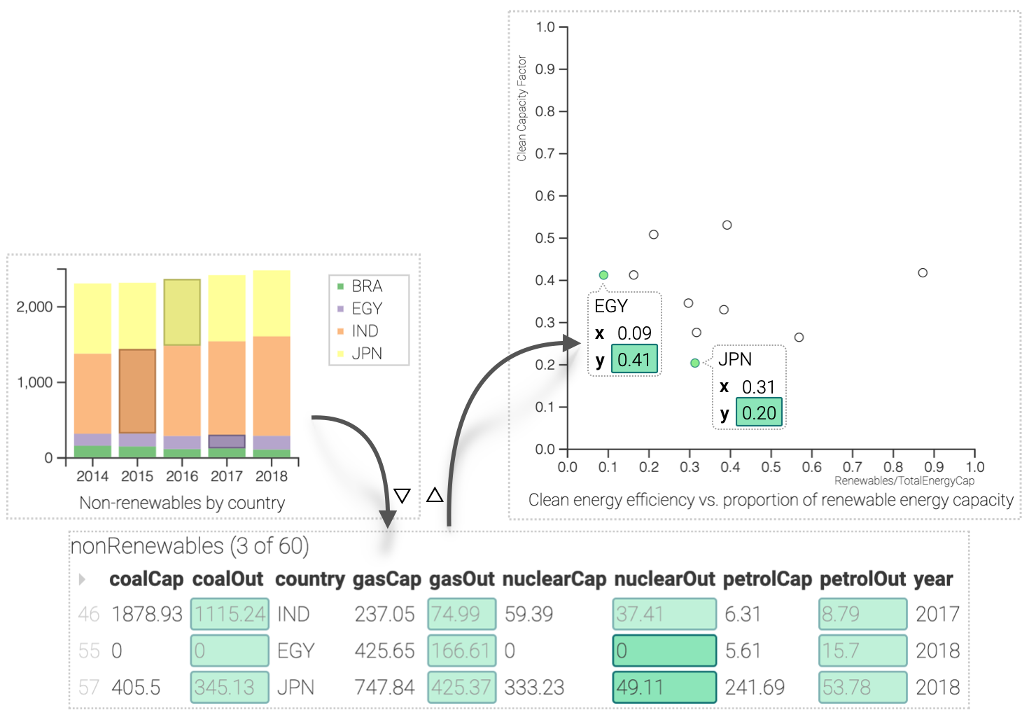
Figure 2. Data-transparent visualisations associate visual selections with demanded data

We call this broad idea of fine-grained in situ provenance queries data transparency, and illustrate this in Figure 2 using our implementation, which builds on these provenance-inspired approaches. Consider the two charts at the top of the figure. As with the histogram, there are many questions even a domain expert might have about these charts. For example, in renewable energy one must be careful not to confuse capacity with output – which of these is being shown in the bar chart? What kinds of energy count as “non-renewable”? In the scatter plot, the label on the x-axis suggests that it represents some kind of part-to-whole ratio (renewables to total energy capacity, perhaps), whereas the y-axis purports to represent the “capacity factor” of clean energy sources. But these labels are little more than informal commentary. Moreover there are two outputs here and so the question of if and how they might be related also arises.

A system with automated data transparency allows the user to investigate questions like these by interacting directly with the artefacts. By selecting an interesting part of the output, they can obtain a view of the relevant data. On the left, the three bar segments highlighted with a dark border indicate such a selection; the table underneath shows the demanded data (computed using our version of the $\displaystyle\triangledown$ operator) and we are also able to automatically select any outputs in the other chart which demand any of the same data using an other operator $\displaystyle\triangle$ (“demanded by”). The overlapping demand , which we call the mediating input, is highlighted using a darker shade of green in Figure 2. Perera et al defined such a $\displaystyle\triangle$ operator as the De Morgan dual of the “suffices for” operator $\displaystyle\blacktriangle$; one of our contributions here is to show that $\displaystyle\triangle$ can be computed in a more direct fashion using dependence graphs.

1.2. Contributions

In this paper, we develop the idea of data transparency in two new directions. First we approach the problem in a language-independent way, using dynamic dependence graphs. This separates the definition of queries over the I/O dependencies for a particular program from the problem of generating a dependence graph for that program. Dependence graphs are a proven technique which have been used extensively for program slicing (mainly of imperative programs (Ferrante et al., 1987)), but have not yet been applied to data analyses based on adjoint pairs of operators (such as $\displaystyle\triangledown$ and $\displaystyle\blacktriangle$). These analyses (e.g. Ricciotti et al. (2017)) have instead utilised a bidirectional interpreter that builds an execution record in the form of a trace during a forwards execution, folding that trace back into a program slice during a backwards execution. This method is quite inefficient and non-trivial to prove correct; instead, we show that a graph-based approach factors the problem into a (language-specific) graph-building interpreter plus (language-agnostic) adjoint analyses over the graph. This partitioning reduces the implementation burden and improves performance compared to approaches based on bidirectional interpretation.

Second, we introduce a new kind of provenance query called related inputs, a relation of mutual relevance which arises between inputs when they contribute to common features of the output. Users are able to formulate queries like “What outputs use this data element, and what other data elements are used along with it?”. Such questions explore cognacy (common ancestry) in a dependence graph $\displaystyle G$, and are formally dual to the “related outputs” feature shown in Figure 2, which can be understood as cognacy in $\displaystyle G^{-1}$. In the graphical setting, these are both easy to compute, since they amount to the two ways of composing reachability in $\displaystyle G$ with its relational converse.

Roadmap

§ 2 presents an overview of our approach and language, and motivates the idea of “related inputs” queries from an end-user perspective. The rest of the paper is organised as follows:

• § 3 defines a new program analysis framework over dynamic dependence graphs, introducing the cognacy operator $\displaystyle{\triangledown}\!{\triangle}$ (“related inputs”) and unpacking the intuitive relationship between its two components $\displaystyle\triangledown$ (“demands”) and $\displaystyle\triangle$ (“demanded by”) in terms of Jonsson and Tarski’s notion of conjugate operators over Boolean algebras. We also introduce the dual cognacy operator $\displaystyle{\triangle}\!{\triangledown}$ (“related outputs”) and explain the relationship to Galois connections: $\displaystyle f$ and $\displaystyle g$ being conjugate is equivalent to $\displaystyle f$ and the De Morgan dual of $\displaystyle g$ forming a Galois connection. We give procedures for computing $\displaystyle\triangledown_{R}$ and $\displaystyle\blacktriangle_{R}$ over a directed graph with reachability relation $\displaystyle R$.

• § 4 defines a core functional language with an operational semantics that pairs every result with a dynamic dependence graph suitable for computing $\displaystyle\triangledown$ and $\displaystyle\triangle$. We show how to represent (parts of) values as vertices in the graph.

• § 5 compares the performance of our implementation based on graphs and conjugates with an implementation due to Perera et al. (2022) based on traces and Galois connections, contrasting the overhead of building trace vs. building dependence graphs, computing $\displaystyle\triangledown$ and $\displaystyle\triangle$ over each, and the relative implementation burden of the two approaches.

• § 6 reviews related work in more detail, including program slicing and DDGs.

• § 7 wraps up with a discussion of some limitations. In particular, the sort of transparency infrastructure proposed in this paper is purely extensional and falls short of providing full explanations of how output parts are related to input parts. We discuss extending this to more “intensional” forms transparency and propose some other ways in which the present system could be improved.

2. Overview of Approach and Solution

As outlined in § 1, the idea of data-transparent outputs is to enrich computed content with interactions that allow the user to query relationships between data sources and visualisations and other outputs in situ, i.e. within the “comprehension context” in which these sorts of questions naturally arise. Crucially, we want to make this feature automatic. Hand-crafted efforts like Bremer and Ranzijn (2015)’s are not only labour-intensive, but involve manually embedding metadata about the relationship between visual outputs and inputs into the same program. The validity of this metadata is fragile: whenever the visualisation or data analysis logic changes, the relationships between inputs and outputs also change. By shifting the responsibility for gathering this information into the programming language, the author or data scientist can concern themselves purely with analysis and visualisation, and defer the provision of these transparency features to the infrastructure used to implement and host the visualisation.

However, computing the bidirectional dependency information needed to realise this idea is costly both in terms of performance and implementation burden. For example, the approach taken by Perera et al. (2022) to implement a “related outputs” analysis like the one shown in Figure 2 requires two separate analyses: a backwards “demands” analysis to determine data needed by an output selection, and a forwards “suffices for” analysis whose De Morgan dual determines any parts of the other chart that also need any of that data. These analyses need to be defined separately and each depends on details of the language, imposing a significant burden on the implementor. Moreover each runs over an execution record or trace of the entire computation regardless of whether all of the trace is relevant.

2.1. Conjugate Operators over Dependence Graphs

Our insight in this paper is that dependence graphs provide an alternative, more language-agnostic foundation for data transparency that both improves performance and reduces the implementation burden. Moreover, certain problems are much easier to formulate in the graphical setting. For example “related outputs” simply amounts to computing common ancestry, or cognacy, in $\displaystyle G$, which turns out to be nicely captured by the concept of “conjugate” operators (Jonsson and Tarski, 1951) between Boolean algebras. Switching to the concrete setting of powersets, $\displaystyle f:\mathbb{P}(X)\to\mathbb{P}(Y)$ and $\displaystyle g:\mathbb{P}(Y)\to\mathbb{P}(X)$ are conjugate iff:

$$f(X)\cap Y=\varnothing\iff X\cap g(Y)=\varnothing$$

The canonical example of conjugate operations are the image and preimage functions $\displaystyle R[\cdot]$ and $\displaystyle R^{-1}[\cdot]$ for a relation $\displaystyle R\subseteq X\times Y$. It is not hard to see that if $\displaystyle R^{-1}[Y^{\prime}]$ overlaps with $\displaystyle X^{\prime}$ where $\displaystyle X^{\prime}\subseteq X$ then necessarily $\displaystyle R[X^{\prime}]$ overlaps with $\displaystyle Y^{\prime}$ where $\displaystyle Y^{\prime}\subseteq Y$, and vice versa. Conjugate pairs are also closely related to Galois connections; if $\displaystyle f$ and $\displaystyle g$ are conjugate, then $\displaystyle f$ and the De Morgan dual of $\displaystyle g$ form a Galois connection (which will be explained in more detail in § 3).

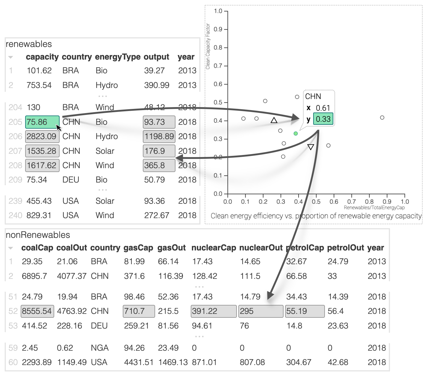
Figure 3. Related inputs are cognate (have a common output dependency)

If we now take $\displaystyle R$ to be reachability in $\displaystyle G$, then our setting technically only requires a single operator $\displaystyle\triangledown_{R}$ (a “demands” relation) to support all the required queries. Its adjoint $\displaystyle\blacktriangle_{R}$ is readily computed as $\displaystyle\triangledown_{R^{-1}}$ and its conjugate $\displaystyle\triangle_{R}$ as the De Morgan dual of $\displaystyle\triangledown_{R^{-1}}$. It is well-known that extensionally any one of these is enough to determine each other, but in the graph setting we can also get the benefit of efficient procedures for all of them in terms of reachability. In particular the “related outputs” relation is simply given by $\displaystyle\triangledown_{R\bbsemi R^{-1}}$. Since going via the De Morgan dual can be inefficient, we also give a direct implementation of $\displaystyle\blacktriangle_{R}$ which improves on the derived version in those cases.

2.2. Related Inputs

Our second insight in this paper is that the graphical setting makes it straightforward to compose reachability in $\displaystyle G$ and with its converse the other way around, producing another provenance query called related inputs ($\displaystyle{\triangledown}\!{\triangle}$). Figure 3 illustrates related inputs, again using our implementation. Here the user starts from one of the input data sets, expressing interest in the bioenergy capacity of China for 2018 by moving their mouse over the appropriate cell in the table (Figure 3 step 1, green selection). The system generates two further selections in response. First, any scatter plot elements that demand the selected input are given a similar green highlight; here just one point is highlighted, and in fact only the $\displaystyle y$ coordinate of that point (step 2, tooltip). We call this output selection the mediating output because of its role in establishing a link between otherwise unrelated inputs.

Finally, any other inputs demanded by the mediating output (i.e. that were needed to compute the $\displaystyle y$ coordinate of that point) are highlighted in grey (steps 3a and 3b). (The grey is used to visually distinguish the answer to the query from the selection that initiated the query in the first place.) The result of a related inputs query can be thought of as a unit of comprehension or unit of reuse. It picks out all the relevant data needed to understand or make use of the original selected input, and does so in a way that identifies the common output elements that explain why the inputs are related. Sometimes a single input is used in many different outputs, or different features of a single output, in which case the query result can be quite noisy (because lots of inputs turn out to be related); in § 3 we also show how selectively projecting away irrelevant parts of the mediating output can refine the query and produce a more precise answer. The same approach can be used to discard irrelevant mediating inputs to obtain more precise results in a related outputs query.

⬇

1let isCountry name x = name == x.country;

2 isYear year x = year == x.year;

3

4let plot year countries =

5 let rens = filter (isYear year) renewables;

6 nonRens = filter (isYear year) nonRenewables;

7 let plotCountry country =

8 let rens’ = filter (isCountry country) rens;

9 rensOut = sum (map (fun x $\displaystyle\rightarrow$ x.output) rens’);

10 rensCap = sum (map (fun x $\displaystyle\rightarrow$ x.capacity) rens’);

11 x = head (filter (isCountry country) nonRens);

12 nonRensCap = x.nuclearCap + x.petrolCap + x.gasCap + x.coalCap

13 in {

14 x: rensCap / (rensCap + nonRensCap),

15 y: (rensOut + x.nuclearOut) / (rensCap + x.nuclearCap)

16 }

17 in map plotCountry countries

18

19in ScatterPlot {

20 caption: "Clean energy efficiency vs. proportion of renewable energy capacity",

21 data: plot 2018 [ "BRA", "CHN", "DEU", "FRA", "EGY", "IND", "JPN", "MEX", "NGA", "USA" ],

22 xlabel: "Renewables/TotalEnergyCap",

23 ylabel: "Clean Capacity Factor"

24}

Figure 4. Source code for scatter plot in Figure 2

2.3. [OurLanguage]: A Data-Transparent Programming Language

We implement the abstract framework outlined above in a programming language called [OurLanguage], a pure functional language with a runtime implementing conjugate dependency operators. From the programmer’s perspective the language is unremarkable; Figure 4 shows the source code for the scatter plot example from Figure 2. The distinguishing feature of the language is a special semantics that interprets a program not as a plain output but as an output with a built-in query engine supporting the transparency features shown above. The author of a visualisation just expresses their chart as a pure function of the inputs, via a set of data types for common visualisations; a d3.js front end automatically enriches the rendered outputs with support for visual selection and various selection-based queries.

In § 3 we set out the formal graph framework and in § 4 show how the [OurLanguage] interpreter implements that abstract framework. Our implementation is open source and available at [anonymised], which also has several interactive demos.

3. Conjugate Operators For Dynamic Dependence Graphs

In this section we introduce Boolean algebras and other preliminaries (§ 3.1); dynamic dependence graphs (§ 3.2), and the image and preimage functions for a relation and their De Morgan duals (§ 3.3). We then extend these operators to dependence graphs (§ 3.4) via their IO relation, and give algorithms for computing them over a given graph (§ 3.5).

3.1. Preliminaries

We give some notation used in the rest of the paper. $\displaystyle X,Y$ range over finite sets.

Finite sequences

Write to $\displaystyle{\vv{x}}$ denote a finite sequence of elements $\displaystyle{x_{1}},\,..,\,{x_{n}}$, with $\displaystyle\epsilon$ as the empty sequence. Concatenation of two sequences $\displaystyle\vv{x}$ and $\displaystyle\vv{x}^{\prime}$ is written $\displaystyle\vv{x}\mathbin{++}\vv{x}^{\prime}$. We also write $\displaystyle x\cdot\vv{x}$ for cons (prepend) and $\displaystyle\vv{x}\cdot x$ for snoc (append).

Finite maps

Write $\displaystyle\{\vv{{k}:{x}}\}$ to denote a set of pairs $\displaystyle{{k_{1}}:{x_{1}}},\,..,\,{{k_{n}}:{x_{n}}}$ where keys $\displaystyle k_{i}$ are pairwise unique.

Disjoint union

Write $\displaystyle X\uplus Y$ to mean $\displaystyle X\cup Y$ where $\displaystyle X$ and $\displaystyle Y$ are disjoint, and also write $\displaystyle x\cdot X$ or $\displaystyle X\cdot x$ to mean $\displaystyle X\uplus\{x\}$. For finite maps $\displaystyle\phi,\psi$ write $\displaystyle\phi\uplus\psi$ to mean $\displaystyle\phi\cup\psi$ where $\displaystyle\textsf{dom}(\phi)$ and $\displaystyle\textsf{dom}(\psi)$ are disjoint.

Relative complement

Write $\displaystyle X\setminus Y$ for the relative complement of $\displaystyle Y$ in $\displaystyle X$, i.e. the set of elements of $\displaystyle X$ that are not in $\displaystyle Y$.

Relational converse

Write $\displaystyle{\cdot}^{-1}$ for the involutive operation that takes a relation $\displaystyle R\subseteq X\times Y$ to its converse $\displaystyle R^{-1}\subseteq Y\times X$ where $\displaystyle(y,x)\in R^{-1}\iff(x,y)\in R$.

3.1.1. Boolean algebras

A Boolean algebra (or Boolean lattice) is a 6-tuple $\displaystyle A=(A,\wedge,\vee,\bot,\top,\neg)$ with carrier $\displaystyle A$, distinguished elements bottom ($\displaystyle\bot$) and top ($\displaystyle\top$), commutative operations meet ($\displaystyle\wedge$) and join ($\displaystyle\vee$) with $\displaystyle\top$ and $\displaystyle\bot$ as respective units, and a unary operation negate ($\displaystyle\neg$) satisfying $\displaystyle x\vee\neg x=\top$ and $\displaystyle x\wedge\neg x=\bot$. The operations $\displaystyle\wedge$ and $\displaystyle\vee$ distribute over each other and induce a partial order $\displaystyle\leq$ over $\displaystyle X$.

Often we will be considering a specific finite Boolean algebra, namely the powerset $\displaystyle\mathbb{P}(X)$ whose carrier is the set of subsets $\displaystyle X^{\prime}\subseteq X$ ordered by inclusion $\displaystyle\subseteq$. Bottom is the empty set $\displaystyle\varnothing$, top is the whole set $\displaystyle X$, meet and join are given by $\displaystyle\cap$ and $\displaystyle\cup$ and negation by relative complement, so that $\displaystyle\neg X^{\prime}=X\setminus X^{\prime}$.

3.2. Dynamic Dependence Graphs

We explain how we arrive at specific dependence graphs in § 4, and here just introduce the basic notion. A dynamic dependence graph (Agrawal and Horgan, 1990) is a directed acyclic graph $\displaystyle G=(V,E)$ with a set $\displaystyle V$ of vertices and set $\displaystyle E\subseteq V\times V$ of edges. In the dependence graph for a particular program, vertices $\displaystyle\alpha,\beta\in V$ represents parts of values (either supplied to the program as inputs or produced during evaluation) and edges $\displaystyle(\alpha,\beta)\in E$ indicate that, in the evaluation of the program, the partial value associated to $\displaystyle\beta$ depends on on the partial value associated to $\displaystyle\alpha$. (The notion of a “part” of a value will be made precise in § 4.) This diverges somewhat from traditional approaches to dynamic dependence graphs in only considering one type of edge (data dependency) rather than separate data and control dependencies; moreover our edges point in the direction of dependent vertices, whereas in the literature the other direction is somewhat more common.

Definition 3.1 (In-edges and out-edges).

For a graph $\displaystyle G=(V,E)$ and vertex $\displaystyle\alpha\in V$, write $\displaystyle\textup{{inE}}_{G}(\alpha)$ for the in-edges of $\displaystyle\alpha$ in $\displaystyle G$ and $\displaystyle\textup{{outE}}_{G}(\alpha)$ for its out-edges.

Definition 3.2 (Sources and sinks).

For a graph $\displaystyle G=(V,E)$, write $\displaystyle S(G)$ for the sources of $\displaystyle G$ (i.e. those vertices with no in-edges) and $\displaystyle T(G)$ for the sinks of $\displaystyle G$ (those with no out-edges).

Definition 3.3 (Reachability relation).

Define the reachability relation for a graph $\displaystyle G=(V,E)$ to be the reflexive transitive closure of $\displaystyle E$.

Definition 3.4 (Opposite graph).

For a graph $\displaystyle G$ define the opposite graph $\displaystyle G^{-1}:=(V,E^{-1})$ where $\displaystyle\cdot^{-1}$ denotes relational converse.

(Taking the opposite graph has the effect of swapping sources and sinks.)

3.2.1. IO Relation for a Graph

Reachability in $\displaystyle G$ induces a relation just between sources and sinks, which we call the IO relation of $\displaystyle G$.

Definition 3.5 (IO relation).

For any dependence graph $\displaystyle G$ with reachability relation $\displaystyle R$, define the IO relation of $\displaystyle G$ to be $\displaystyle R\cap(S(G)\times T(G))$.

The IO relation specifies how specific inputs (sources) are demanded by specific outputs (sinks); thus we will interpret $\displaystyle(x,y)\in R$ as “$\displaystyle x$ is demanded by $\displaystyle y$”. Clearly the IO relation of $\displaystyle G$ is the converse of the IO relation of $\displaystyle G^{-1}$. Since we are in fact interested in the relationship between input and outputs selections (namely sets of inputs and outputs), we now consider how such a relation $\displaystyle R\subseteq X\times Y$ lifts to $\displaystyle\mathbb{P}(X)$ and $\displaystyle\mathbb{P}(Y)$ via the image and preimage functions for $\displaystyle R$, which we will denote using $\displaystyle\triangle$ and $\displaystyle\triangledown$.

3.3. Conjugate Image and Preimage Functions

Definition 3.6 (Image and Preimage Functions for a Relation).

For a relation $\displaystyle R\subseteq X\times Y$, define $\displaystyle\triangle_{R}:\mathbb{P}(X)\to\mathbb{P}(Y)$ and $\displaystyle\triangledown_{R}:\mathbb{P}(Y)\to\mathbb{P}(X)$ as:

1. $\displaystyle\triangle_{R}(X^{\prime}):=\{y\in Y\mid\exists x\in X^{\prime}.(x,y)\in R\}$ (image)

2. $\displaystyle\triangledown_{R}(Y^{\prime}):=\{x\in X\mid\exists y\in Y^{\prime}.(x,y)\in R\}$ (preimage)

Clearly the image function for $\displaystyle R$ is the preimage function for its converse; this is important enough to state as a lemma:

Lemma 3.7 (Image as Preimage of Converse Relation).

$\displaystyle\triangle_{R}=\triangledown_{R^{-1}}$

When thinking of $\displaystyle R$ as an IO relation, the image $\displaystyle\triangle_{R}(X^{\prime})$ consists of all outputs that any element of $\displaystyle X^{\prime}$ is demanded by, and the preimage $\displaystyle\triangledown_{R}(Y^{\prime})$ consists of all inputs demanded by any element of $\displaystyle Y^{\prime}$. If $\displaystyle R$ happens to be a function, the image and preimage functions form a Galois connection (Definition 3.12 below); for a proper relation they form a conjugate pair, in the sense of Jonsson and Tarski (1951):

Definition 3.8 (Conjugate Functions).

For Boolean algebras $\displaystyle A$, $\displaystyle B$, functions $\displaystyle f:A\to B$ and $\displaystyle g:B\to A$ form a conjugate pair iff:

$$f(x)\wedge y=\bot\iff x\wedge g(y)=\bot$$

(Jonsson and Tarski consider only endofunctions; here we extend the idea of conjugacy to maps between Boolean algebras.)

Lemma 3.9 (Preimage and Image of a relation are conjugate).

For any relation $\displaystyle R\subseteq X\times Y$ the functions $\displaystyle\triangle_{R}$ and $\displaystyle\triangledown_{R}$ are conjugate.

This should be intuitive enough: for any subsets $\displaystyle X^{\prime}\subseteq X$ and $\displaystyle Y^{\prime}\subseteq Y$, if the elements “on the right” to which $\displaystyle X^{\prime}$ is related are disjoint from $\displaystyle Y^{\prime}$, then there are no edges in $\displaystyle R$ from $\displaystyle X^{\prime}$ to $\displaystyle Y^{\prime}$; and in virtue of that, the elements “on the left” to which $\displaystyle Y^{\prime}$ is related must also be disjoint from $\displaystyle X^{\prime}$.

3.3.1. Dual Image and Preimage Functions

If $\displaystyle R$ is an IO relation, then $\displaystyle\triangle_{R}(X)$ effectively asks “what is $\displaystyle X$ necessary for?” This naturally leads to the question “what is $\displaystyle X$ sufficient for?” In fact, we can use the notion of sufficiency as a test of correctness. If we begin by selecting an output of interest, we would expect the data it demands to also be sufficient to reconstruct it. This leads us to define the following pair of functions, which also form a conjugate pair.

Definition 3.10 (Dual Image and Preimage Functions for a Relation).

For any relation $\displaystyle R\subseteq X\times Y$, define $\displaystyle\blacktriangle_{R}:\mathbb{P}(X)\to\mathbb{P}(Y)$ and $\displaystyle\blacktriangledown_{R}:\mathbb{P}(Y)\to\mathbb{P}(X)$ as the composition:

1. $\displaystyle\blacktriangle_{R}(X^{\prime}):=\{y\in Y\mid\nexists x\in X\setminus X^{\prime}.(x,y)\in R\}$ (dual image)

2. $\displaystyle\blacktriangledown_{R}(Y^{\prime}):=\{x\in X\mid\nexists y\in Y\setminus Y^{\prime}.(x,y)\in R\}$ (dual preimage)

This definition is similar to $\displaystyle\triangle_{R}$ except that $\displaystyle\blacktriangle_{R}$ needs every ancestor to be in the input set, rather than any ancestor to be in the input set. We can, in fact, turn this query on sufficiency into $\displaystyle\triangle_{R}$, using the De Morgan Dual.

Definition 3.11 (De Morgan Dual).

Suppose a function $\displaystyle f:A\to B$ between Boolean algebras with $\displaystyle\neg_{A}$ and $\displaystyle\neg_{B}$ the negation operators of $\displaystyle A$ and $\displaystyle B$. Define the De Morgan Dual $\displaystyle f^{\circ}:A\to B$ of $\displaystyle f$ as:

$$f^{\circ}:=\neg_{B}\circ f\circ\neg_{A}$$

Definition 3.12 (Galois connection).

Suppose $\displaystyle A,B$ are partial orders. Then monotone functions $\displaystyle f:A\to B$ and $\displaystyle g:B\to A$ form a Galois connection iff

$$f(x)\leq y\iff x\leq g(y)$$

Proposition 3.13 (Correspondence Between Conjugates and Galois Connections).

Suppose functions $\displaystyle f:A\to B$ and $\displaystyle g:B\to A$ between Boolean algebras. The following statements are equivalent:

1. $\displaystyle f$ and $\displaystyle g$ form a conjugate pair

2. $\displaystyle f$ and $\displaystyle g^{\circ}$ form a Galois connection

Lemma 3.14 (Duality of image and preimage functions).

1. $\displaystyle\triangle_{R}^{\circ}=\blacktriangle_{R}$

2. $\displaystyle\triangledown_{R}^{\circ}=\blacktriangledown_{R}$

3.4. $\displaystyle\triangledown$ and $\displaystyle\triangle$ over Dependence Graphs

We now extend the notion of $\displaystyle\triangledown$ and $\displaystyle\triangle$ to a dependence graph $\displaystyle G$ via its IO relation. The set of outputs demanded by some inputs $\displaystyle X$ is simply the subset of the outputs of $\displaystyle G$ reachable from $\displaystyle X$, i.e. the intersection of $\displaystyle\triangle_{R}(X)$ with $\displaystyle T(G)$. Conversely, the set of inputs that some outputs $\displaystyle Y$ demands is simply the subset of the inputs of $\displaystyle G$ reachable from $\displaystyle Y$ by traversing the graph in the opposite direction, i.e. the intersection of $\displaystyle\triangledown_{R}$ with $\displaystyle S(G)$.

Definition 3.15 ($\displaystyle\triangledown$ and $\displaystyle\triangle$ for a dependence graph).

For a graph $\displaystyle G$ with IO relation $\displaystyle R$, define:

1. $\displaystyle\triangle_{G}:=\triangle_{R}:\mathbb{P}(S(G))\to\mathbb{P}(T(G))$ (demanded by)

2. $\displaystyle\triangledown_{G}:=\triangledown_{R}:\mathbb{P}(T(G))\to\mathbb{P}(S(G))$ (demands)

3.5. Computing $\displaystyle\triangledown_{G}$ and $\displaystyle\triangle_{G}$ and their duals

We now show how to compute $\displaystyle\triangle_{G}$ and $\displaystyle\triangledown_{G}$ and their duals $\displaystyle\blacktriangle_{G}$ and $\displaystyle\blacktriangledown_{G}$ for a dependence graph $\displaystyle G$. One advantage of graphs over the trace-based approach of Perera et al. (2022) is that a single algorithm can be readily adapted to compute all 4 operators; given a procedure for $\displaystyle\triangle_{G}$, for example, we can compute its conjugate $\displaystyle\triangledown_{G}$ as $\displaystyle\triangle_{G^{-1}}$ (by Lemma 3.7) and its dual $\displaystyle\blacktriangle_{G}$ by pre- and post-composing with negation (Definition 3.11).

For efficiency, however, we give a direct procedure both for $\displaystyle\triangle_{G}$ (§ 3.5.1) and $\displaystyle\blacktriangle_{G}$ (§ 3.5.2), allowing us to compute the other two operators via the opposite graph; this is in some situations more efficient than relying on the De Morgan dual, which can cause more graph to be traversed than would be otherwise. Both procedures factor through an auxiliary operation that computes a “slice” of the original graph, i.e. a contiguous subgraph. While it is technically possible to compute the desired image/preimage of the IO relation without creating this intermediate graph, we anticipate many use cases which will make use of the graph slice; these are discussed in more detail in § 7. Our implementation makes it easy to flip between $\displaystyle G$ and $\displaystyle G^{-1}$ so we freely make use of both in the algorithms to access out-neighbours and in-neighbours.

An alternative presentation of graphs in terms of adjacency maps is useful notationally.

Definition 3.16 (Graph as adjacency map).

A graph $\displaystyle G=(V,E)$ can also be specified as an adjacency map $\displaystyle G:V\to\mathbb{P}(V)$ from vertices to sets of out neighbours, where

$$G(\alpha)=V^{\prime}\iff\alpha\in V\text{ and }\forall\beta\in V^{\prime}.(\alpha,\beta)\in E$$

3.5.1. Direct algorithm for $\displaystyle\triangle_{G}$ (demanded by)

Definition 3.17 ($\displaystyle\mathrel{\textup{{demBy}}_{G}}$).

Figure 5(a) defines the family of relations $\displaystyle\mathrel{\textup{{demBy}}_{G}}$ for dependence graph $\displaystyle G$.

$\displaystyle X\mathrel{\textup{{demBy}}_{G}}Y$ *[ right=$\displaystyle X\subseteq S(G)$ ] (∅, ∅), X demByV_G G’ X demBy_G V(G’) ∩T(G)

$\displaystyle G^{\prime},X\mathrel{\textup{{demByV}}_{G}}G^{\prime\mkern-2.6mu\prime\mkern-2.2mu}$ *[ lab=done, right=$\displaystyle G^{\prime}\subseteq G$ ] G’, ∅demByV_G G’ *[ lab=skip, right=$\displaystyle\alpha\in\textup{{V}}(G)$ ] G’, X demByV_G G^′′ G’, α⋅X demByV_G G^′′ *[ lab=extend, right=$\displaystyle H=\{{\alpha}:{Y}\}$ ] G’ ⊎H, Y ⊎X demByV_G ⊎H G^′′ G’, α⋅X demByV_G ⊎H G^′′

(a) $\displaystyle\mathrel{\textup{{demBy}}}$ algorithm

$\displaystyle X\mathrel{\textup{{suff}}_{G}}U$

* (X, ∅), ∅, {(α, β) ∈outE_G(α’) ∣α’ ∈X} suffE_G G’, H X suff_G V(G’) ∩S(G)

$\displaystyle G^{\prime},H,E\mathrel{\textup{{suffE}}_{G}}G^{\prime\mkern-2.6mu\prime\mkern-2.2mu},H^{\prime}$

*[ lab=done, right=$\displaystyle G^{\prime}\subseteq G^{-1}$ ] G’, H, ∅suffE_G G’, H *[ lab=pending, right=$\displaystyle H^{\prime}=H\cup\{{\beta}:{\{\alpha\}}\}$ ] H’(β) ⊂G^-1(β)
G’, H’, E suffE_G G^′′, H^′′ G’, H, (α, β) ⋅E suffE_G G^′′, H^′′ *[ lab=extend, right=$\displaystyle H^{\prime}=H\cup\{{\beta}:{\{\alpha\}}\}$ ] H’(β) = G^-1(β)
G’ ⊎{β:H’(β)}, H ∖{β}, outE_G(β) ⊎E suffE_G G^′′, H^′′ G’, H, (α, β) ⋅E suffE_G G^′′, H^′′

(b) $\displaystyle\mathrel{\textup{{suff}}}$ algorithm

Figure 5. Dual analyses over a dependence graph $\displaystyle G$

For a dependence graph $\displaystyle G$ and inputs $\displaystyle X\subseteq S(G)$, the judgement $\displaystyle X\;\smash{\mathrel{\textup{{demBy}}_{G}}}Y$ says that $\displaystyle X$ is demanded by $\displaystyle Y\subseteq T(G)$. It is possible to read an algorithm directly from the inductive definition, treating it as a function with $\displaystyle V$ and index $\displaystyle G$ as inputs. The auxiliary operation $\displaystyle G\mathrel{\textup{{demByV}}_{G}}$ maintains a set of vertices still to process and builds the graph slice $\displaystyle G^{\prime}\subseteq G$ consisting of all vertices reachable from the initial set and all edges between them. If $\displaystyle X$ is empty (done) the graph slice $\displaystyle G^{\prime}$ is complete and can be returned. Otherwise we select an arbitrary vertex $\displaystyle\alpha$ from $\displaystyle X$. If $\displaystyle\alpha$ is already in $\displaystyle G^{\prime}$ (skip), there is nothing to do at this step and we continue with the remaining vertices. Otherwise, we add the out-star at $\displaystyle\alpha$ to $\displaystyle G^{\prime}$ and the out-neighbours to the pending vertices (extend). When $\displaystyle\mathrel{\textup{{demByV}}}$ is done, $\displaystyle\mathrel{\textup{{demBy}}}$ extracts the output set from the graph slice by intersecting with $\displaystyle T(G)$.

Proposition 3.18 ($\displaystyle\mathrel{\textup{{demBy}}}$ Computes $\displaystyle\triangle$).

For any dependence graph $\displaystyle G$, any $\displaystyle X\subseteq S(G)$ and any $\displaystyle Y\subseteq T(G)$ we have

$$X\mathrel{\textup{{demBy}}_{G}}Y\iff\triangle_{G}(X)=Y$$

3.5.2. Direct algorithm for $\displaystyle\blacktriangle_{G}$ (suffices)

Definition 3.19 ($\displaystyle\mathrel{\textup{{suff}}_{G}}$).

Figure 5(b) defines the family of relations $\displaystyle\mathrel{\textup{{suff}}_{G}}$ for dependence graph $\displaystyle G$.

For a dependence graph $\displaystyle G$, the algorithm $\displaystyle\mathrel{\textup{{suff}}}$ also delegates to an auxiliary procedure $\displaystyle\mathrel{\textup{{suffE}}}$ which builds a graph slice $\displaystyle G$’, similar to $\displaystyle\mathrel{\textup{{demands}}}$ except that the direction of the slice is inverted, i.e. $\displaystyle G^{\prime}\subseteq G^{-1}$. The judgement $\displaystyle\mathrel{\textup{{suffE}}}$ takes the graph slice under construction $\displaystyle G^{\prime}$, a “pending” subgraph $\displaystyle H\subseteq G$ with $\displaystyle S(H)\subseteq T(G^{\prime})$, and the current set of edges under consideration $\displaystyle E$. For efficiency, the algorithm traverses each edge in the graph at most once.

Figure 6 shows an example run of the algorithm. Green vertices have been included into $\displaystyle G^{\prime}$ because all of their in-edges in $\displaystyle G$ are out-edges in $\displaystyle G^{\prime}$; orange vertices are “pending”, with at least one in-edge from $\displaystyle G$ as an out-edge in $\displaystyle H$; blue vertices are unvisited. Dashed edges indicate the current edge set $\displaystyle E$. At each step we non-deterministically choose an edge $\displaystyle(\alpha,\beta)$ from $\displaystyle E$ and add the opposite edge $\displaystyle(\beta,\alpha)$ to $\displaystyle H$ (dotted edges in steps 2 and 3). If the out-neighbours of $\displaystyle\beta$ in $\displaystyle H$ are now equal to its in-neighbours in $\displaystyle G$ (as in step 3), we move that out-star from $\displaystyle H$ to $\displaystyle G$ and add the in-edges of $\displaystyle\beta$ in $\displaystyle G$ to $\displaystyle E$ ($\displaystyle\mathrel{\textup{{suffE}}}$-extend, step 4). Otherwise, there is nothing more to do at this step and we continue with the remaining edges in $\displaystyle E$ ($\displaystyle\mathrel{\textup{{suffE}}}$-pending). The algorithm terminates when $\displaystyle E$ is empty ($\displaystyle\mathrel{\textup{{suffE}}}$-done); any vertices still pending in $\displaystyle H$ (as in step 8) are vertices had only partially sufficient inputs.

Figure 6. Run of $\displaystyle\mathrel{\textup{{suff}}}$ with $\displaystyle G$ and $\displaystyle H$ superimposed on $\displaystyle G_{0}$

Proposition 3.20 ($\displaystyle\mathrel{\textup{{suff}}}$ Computes $\displaystyle\blacktriangle$).

For any dependence graph $\displaystyle G$, any $\displaystyle X\subseteq S(G)$ and any $\displaystyle Y\subseteq T(G)$ we have:

$$X\mathrel{\textup{{suff}}_{G}}Y\iff\blacktriangle(X)=Y$$

3.5.3. Derived algorithms

Propositions 3.18 and 3.20 justify treating $\displaystyle\mathrel{\textup{{demBy}}_{G}}$ and $\displaystyle\mathrel{\textup{{suff}}_{G}}$ as functions. Using Lemma 3.14 we can define direct algorithms for $\displaystyle\triangledown_{G}$ and $\displaystyle\blacktriangledown_{G}$ from $\displaystyle\mathrel{\textup{{demBy}}_{G}}$ and $\displaystyle\mathrel{\textup{{suff}}_{G}}$ by simply flipping the graph; using Lemma 3.14 and Definition 3.11 we can also define alternative algorithms for all 4 operators using the De Morgan dual construction. All algorithms are summarised in Figure 7.

Abstract operator	Direct algorithm	Alternative algorithm
$\displaystyle\triangle_{G}$	$\displaystyle\mathrel{\textup{{demBy}}_{G}}$	$\displaystyle\mathrel{\textup{{suff}}_{G}}^{\circ}$
$\displaystyle\triangledown_{G}$	$\displaystyle\mathrel{\textup{{demBy}}_{G^{-1}}}$	$\displaystyle\mathrel{\textup{{suff}}_{G^{-1}}}^{\circ}$
$\displaystyle\blacktriangle_{G}$	$\displaystyle\mathrel{\textup{{suff}}_{G}}$	$\displaystyle\mathrel{\textup{{demBy}}_{G}}^{\circ}$
$\displaystyle\blacktriangledown_{G}$	$\displaystyle\mathrel{\textup{{suff}}_{G^{-1}}}$	$\displaystyle\mathrel{\textup{{demBy}}_{G^{-1}}}^{\circ}$

Figure 7. Direct and alternative (De Morgan Dual) algorithms for all 4 operators

In § 5 we contrast the performance of the direct and De Morgan dual implementations of $\displaystyle\triangle_{G}$, which is an essential component of the related inputs and related outputs operators introduced in § 2.

3.6. $\displaystyle{\triangledown}\!{\triangle}$ and $\displaystyle{\triangle}\!{\triangledown}$ over dependence graphs

Now we can provide a formal account of the notions of related inputs and related outputs.

Definition 3.21 (Related Inputs and Outputs).

For a dependence graph $\displaystyle G$ define:

1. $\displaystyle{\triangledown}\!{\triangle}_{G}:=\triangledown_{G}\circ\triangle_{G}$ (related inputs)

2. $\displaystyle{\triangle}\!{\triangledown}_{G}:=\triangle_{G}\circ\triangledown_{G}$ (related outputs)

Intuitively, related outputs and related inputs are relations of cognacy (common ancestry) in $\displaystyle G$ and $\displaystyle G^{-1}$ respectively. For a set of inputs $\displaystyle X\subseteq S(G)$, related inputs asks “what other inputs are demanded by the outputs which demand X?”, and first finds all outputs $\displaystyle\triangle_{G}(X)$ that our inputs are demanded by, and then computes the inputs that those outputs demand, i.e. $\displaystyle\triangledown_{G}(\triangle_{G}(X^{\prime}))$. For a set of outputs $\displaystyle Y\subseteq T(G)$, related outputs asks “what other outputs demand the inputs that Y demands”, and first finds all inputs $\displaystyle\triangledown_{G}(Y^{\prime})$ that our outputs demand, and then computes the outputs that those inputs $\displaystyle\triangledown_{G}(Y)$ demand, i.e. $\displaystyle\triangle_{G}(\triangledown_{G}(Y))$.

Neither $\displaystyle{\triangledown}\!{\triangle}_{G}$ nor $\displaystyle{\triangle}\!{\triangledown}_{G}$ is necessarily inflationary, as illustrated in Figure 8. In Figure 8(a), the uppermost vertex on the left is part of the initial input selection $\displaystyle X^{\prime}$, but is not preserved by the $\displaystyle\triangledown_{G}\circ\triangle_{G}$ round-trip because it is not demanded by any output. In Figure 8(b), the uppermost vertex on the right is part of the initial output selection $\displaystyle Y^{\prime}$, but is not preserved by the $\displaystyle\triangle_{G}\circ\triangledown_{G}$ round-trip because it does not demand any input.

(a) $\displaystyle{\triangledown}\!{\triangle}_{R}$

(b) $\displaystyle{\triangle}\!{\triangledown}_{R}$

Figure 8. In general neither $\displaystyle{\triangledown}\!{\triangle}_{R}$ nor $\displaystyle{\triangle}\!{\triangledown}_{R}$ is inflationary

If we constrain things so that there are no inputs which are unused, then $\displaystyle\triangledown$ will preserve $\displaystyle\bot$, i.e. $\displaystyle\triangledown(\varnothing)=\varnothing$, and $\displaystyle{\triangle}\!{\triangledown}_{G}$ will preserve the original output selection. Similarly, if we constrain things so that all outputs demand some input, then $\displaystyle\triangle$ will preserve $\displaystyle\bot$, and $\displaystyle{\triangledown}\!{\triangle}_{G}$ will preserve the original input selection:

Lemma 3.22.

1. If $\displaystyle\triangle_{G}(\varnothing)=\varnothing$, then for all $\displaystyle X$ we have $\displaystyle{\triangledown}\!{\triangle}_{G}(X)\geq X$.

2. If $\displaystyle\triangledown_{G}(\varnothing)=\varnothing$, then for all $\displaystyle Y$ we have $\displaystyle{\triangle}\!{\triangledown}_{G}(Y)\geq Y$.

As an easy corollary, if $\displaystyle\triangledown_{G}$ and $\displaystyle\triangle_{G}$ both preserve $\displaystyle\varnothing$ then in fact they form an antitone Galois connection. These observations have practical implications: for example it is sometimes convenient to consider a filtered view of the data where by default the user only sees data which is actually used somewhere, and in such a setup a related inputs query will never cause any selected data to become unselected.

4. A Core Language with Graphical Syntax and Semantics

In § 3, we defined the abstract setting of dependence graphs and conjugate operators demands ($\displaystyle\triangledown$) and demanded by ($\displaystyle\triangle$) over such graphs. We now implement that graphical abstraction for [OurLanguage], an untyped, pure functional programming language. This core calculus we go on to describe is what underlies the surface-language programs such as Figure 4, used to generate and analyse the scatter plots from earlier. We first introduce the syntax of our core language constructs (§ 4.1). Then we define a big-step operational semantics that simultaneously (i) evaluates a term to a value and (ii) constructs an accompanying dependence graph for the evaluation of that term (§ 4.2); we also address how we deal with pattern-matching and mutual recursion.

4.1. Syntax

	Expression
$\displaystyle e::=$	$\displaystyle x$	variable
	$\displaystyle n$	integer
	$\displaystyle{\text{{let}}}\;{x}\mathrel{{\text{{=}}}}{e}\;{\text{{in}}}\;{e^{\prime}}$	let
	$\displaystyle\{\vv{{x}:{e}}\}$	record
	$\displaystyle e.x$	record projection
	$\displaystyle c(\vv{e})$	constructor
	$\displaystyle{e}\,{e^{\prime}}$	application
	$\displaystyle{f}({\vv{e}})$	foreign application
	$\displaystyle\lambda{\sigma}$	function
	$\displaystyle{\text{{let}}}\;{\vv{{x}:{\sigma}}}\;{\text{{in}}}\;{e}$	recursive let
	Continuation
$\displaystyle\kappa::=$	$\displaystyle e$	expression
	$\displaystyle\sigma$	eliminator

	Eliminator
$\displaystyle\sigma::=$	$\displaystyle{x}\mapsto{\kappa}$	variable
	$\displaystyle{\{{\vv{x}}\}}\mapsto{\kappa}$	record
	$\displaystyle\{\vv{{c}\mapsto{\kappa}}\}$	constructor
	Value
$\displaystyle v::=$	$\displaystyle\bm{v}_{\alpha}$
	Raw value
$\displaystyle\bm{v}::=$	$\displaystyle n$	integer
	$\displaystyle\{\vv{{x}:{v}}\}$	record
	$\displaystyle c(\vv{v})$	constructor
	$\displaystyle{\text{{cl}}}({\gamma},{\rho},{\sigma})$	closure
	Environment
$\displaystyle\gamma::=$	$\displaystyle\{\vv{{x}:{v}}\}$
	Recursive definitions
$\displaystyle\rho::=$	$\displaystyle\{\vv{{x}:{\sigma}}\}$

Figure 9. Syntax of core language, including annotated values

4.1.1. Terms

Figure 9 defines the expressions $\displaystyle e$ of the language, which include variables $\displaystyle x,y,f$; integer constants $\displaystyle n,m$; let-bindings $\displaystyle{\text{{let}}}\;{x}\mathrel{{\text{{=}}}}{e}\;{\text{{in}}}\;{e^{\prime}}$; record construction $\displaystyle\{\vv{{x}:{e}}\}$; and record projection $\displaystyle e.x$. We also have constructor expressions $\displaystyle c(\vv{e})$, where $\displaystyle c$ ranges over data constructors and is fully saturated by arguments $\displaystyle\vv{e}$; we write $\displaystyle\Sigma(c)=n$ to denote that $\displaystyle c$ takes $\displaystyle n\in\mathbb{N}$ arguments. Application comes in two forms: standard application $\displaystyle{e}\,{e^{\prime}}$, and foreign application $\displaystyle{f}({\vv{e}})$ for calling foreign functions which are explained in § 4.1.2. The last two terms define anonymous functions $\displaystyle\lambda{\sigma}$ and (mutually) recursive let-bindings $\displaystyle{\text{{let}}}\;{\vv{x:\sigma}}\;{\text{{in}}}\;{e}$, where $\displaystyle\sigma$ is a pattern-matching construct called an eliminator detailed further in § 4.1.3.

4.1.2. Foreign functions

The language is parameterised by a finite map $\displaystyle\Phi(f)=n$ from variables $\displaystyle f$ to the arities $\displaystyle n\in\mathbb{N}$ of the foreign function they represent (analogous to $\displaystyle\Sigma(c)=n$ for constructors). For the graph semantics that will follow, every foreign function $\displaystyle f$ is required to provide an interpretation $\displaystyle\hat{f}$ that computes both $\displaystyle f$’s result and a suitable dependence graph.

Foreign functions in the core language are not first-class and calls $\displaystyle{f}({\vv{e}})$ are saturated, i.e. $\displaystyle|\vv{e}|=\Phi{(f)}$. In our implementation, which also provides a surface language which desugars into the core, first-class foreign functions are supported via a top-level environment which maps every $\displaystyle{f}$ to the closure $\displaystyle{\text{{cl}}}({\varnothing},{\epsilon},{{x_{1}}\mapsto{{..}\mapsto{{x_{\Phi{(f)}}}\mapsto{{f}({\vv{x}})}}}})$ where $\displaystyle|\vv{x}|=\Phi{(f)}$.

4.1.3. Continuations and eliminators

A continuation $\displaystyle\kappa$ describes how an execution proceeds after a value is pattern-matched, and is either a term $\displaystyle e$ or an eliminator $\displaystyle\sigma$. Eliminators are trie-like objects (Hinze, 2000) that specify how this pattern-matching is done and the subsequent continuation $\displaystyle\kappa$ to be executed under additional variable bindings. (These are what the piecewise function definitions of our surface-language, e.g. plot in Figure 4, desugar into; Peyton Jones et al. (2022) present a similar idea.) A variable eliminator $\displaystyle{x}\mapsto{\kappa}$ says how to match any value (as variable $\displaystyle x$) and continue as $\displaystyle\kappa$. A record eliminator $\displaystyle{\{{\vv{x}}\}}\mapsto{\kappa}$ says how to match a record with fields $\displaystyle\vv{x}$, and provides a continuation $\displaystyle\kappa$ for matching the values of those fields. Lastly, the eliminator $\displaystyle\{\vv{c\mapsto\kappa}\}$ provides a branch $\displaystyle c\mapsto\kappa$ for each constructor $\displaystyle c$ in $\displaystyle\vv{c}$, where each $\displaystyle\kappa$ may specify how the arguments to $\displaystyle c$ will be matched. (We assume that any constructors matched by an eliminator all belong to the same data type, but this is not enforced in the core language.)

4.1.4. Values and environments

We define addressed values $\displaystyle v$ mutually inductively with raw values $\displaystyle\bm{v}$, a raw value does not have an associated address. These addresses, explained in § 4.1.5, will (later) form the vertices of the graphs that we build in the graph semantics.

Raw values $\displaystyle\bm{v}$ include integers $\displaystyle n,m$; records $\displaystyle\{{\vv{x\mapsto v}}\}$; and constructor values $\displaystyle c(\vv{v})$. We also define function closures as $\displaystyle{\text{{cl}}}({\gamma},{\rho},{\sigma})$ where $\displaystyle\sigma$ is the function (eliminator), $\displaystyle\gamma$ is its environment, and to support mutual recursion, $\displaystyle{\rho}$ is the (possibly empty) environment of functions (eliminators) with which $\displaystyle\sigma$ was mutually defined. An environment is defined as a finite map.

4.1.5. Addresses for partial values

The addresses $\displaystyle\alpha$ that annotate values act as identifiers, uniquely corresponding those values to specific vertices in a dependence graph. There are many sensible ways of assigning addresses (our particular implementation uses an integer counter to generate new ones) as long as some freshness condition is satisfied – ensuring that there are no unwanted address collisions in a given value i.e. graph. For simplicity, we elide this side-condition in the graph semantics (next) and assume it is met whenever a new address $\displaystyle\alpha$ is introduced.

4.2. Evaluation and Graph Construction

$\displaystyle\vv{v},\kappa\rightsquigarrow\gamma,e,V$ *[ lab=$\displaystyle\rightsquigarrow$-done ] ϵ, e ↝∅, e, ∅ *[lab=$\displaystyle\rightsquigarrow$-var] v, κ↝γ, e, V v ⋅v, x↦κ ↝γ⋅(x:v), e, V

*[ lab=$\displaystyle\rightsquigarrow$-record ] {y:u} ⊆{x:v}

u ++v’, κ↝γ, e, V {x:v}_α ⋅v’, {y}↦κ ↝γ, e, α⋅V *[lab=$\displaystyle\rightsquigarrow$-constr , right=$\displaystyle\Sigma(c)=|\vv{v}|$] v ++v’, κ↝γ, e, V c(v)_α ⋅v’, (c↦κ) ⋅{c↦κ} ↝γ, e, α⋅V

Figure 10. Pattern-matching

$\displaystyle\gamma,e,V\Rightarrow v,G$ *[ lab=$\displaystyle\Rightarrow$-var ] γ⋅(x:v), x, V ⇒v, ∅ *[ lab=$\displaystyle\Rightarrow$-int ] γ, n, V ⇒n_α, {V α} *[lab=$\displaystyle\Rightarrow$-function] γ, λσ, V ⇒cl(γ,∅,σ)_α, {V α} *[lab=$\displaystyle\Rightarrow$-record] γ, e, V ⇒v, G γ, {x:e}, V ⇒{x:v}_α, G ⊎{V α} *[lab=$\displaystyle\Rightarrow$-constr , right=$\displaystyle\Sigma(c)=|\vv{e}|$] γ, e, V ⇒v, G γ, c(e), V ⇒c(v)_α, G ⊎{V α} *[ lab=$\displaystyle\Rightarrow$-record-project ] γ, e, V ⇒{x:v ⋅(y:u)}_α, G γ, e.y, V ⇒u, G *[ lab=$\displaystyle\Rightarrow$-foreign-app , right=$\displaystyle\Phi(f)=|\vv{e}|$] γ, e, V ⇒v, G

^f

(v) = (u, G’) γ, f(e), V ⇒u, G ⊎G’ *[ lab=$\displaystyle\Rightarrow$-let ] γ, e, V ⇒v, G

γ⋅(x:v), e’, V ⇒v’, G’ γ, let x=e in e’, V ⇒v’, G ⊎G’ *[ lab=$\displaystyle\Rightarrow$-let-rec ] γ, {x:σ}, V ↣γ’, G

γ++γ’, e, V ⇒v, G’ γ, let x:σ in e, V ⇒v, G ⊎G’ *[ lab=$\displaystyle\Rightarrow$-app, width=4in, ] γ, e, V ⇒cl(γ_1,ρ,σ)_α, G_1

γ_1, ρ, {α} ↣γ_2, G_2

γ, e’, V ⇒v’, G_3       v’, σ↝γ_3, e^′′, V’       γ_1 ++γ_2 ++γ_3, e^′′, V’ ⊎{α} ⇒u, G_4 γ, e e’, V ⇒u, ⨄{G1 ,  ..,  G4}

$\displaystyle\gamma,\vv{e},V\Rightarrow\vv{v},G$ *[ lab=$\displaystyle\Rightarrow$-seq ] γ, e_i, V ⇒v_i, G_i

(∀i ≤—e—) γ, e, V ⇒v, ⨄ G

Figure 11. Operational semantics: evaluation and graph construction

$\displaystyle\gamma,\rho,V\rightarrowtail\gamma^{\prime},G$ with $\displaystyle\textsf{dom}(\gamma^{\prime})=\textsf{dom}(\rho)$ *[] v_i = cl(γ,ρ,ρ(x_i))_α_i

G_i = {α_i:V}  (∀i ≤—x—) γ, ρ, V ↣{x:v}, ⨄G

Figure 12. “Closing over” recursive definitions

4.2.1. Pattern matching

Figure 10 defines the pattern-matching judgement $\displaystyle\vv{v},\kappa\rightsquigarrow\gamma,e,V$. Rather than matching a single value $\displaystyle v$ against an eliminator $\displaystyle\sigma$, the judgement matches a “stack” of values $\displaystyle\vv{v}$ against a continuation $\displaystyle\kappa$. It then returns the selected branch $\displaystyle e$, an environment $\displaystyle\gamma$ providing bindings for the free variables in $\displaystyle e$, and a set $\displaystyle V$ of vertices found in the matched portions of $\displaystyle\vv{v}$.

The $\displaystyle\rightsquigarrow$-done rule expresses exactly when using a term $\displaystyle e$ as the continuation may succeed: when the stack of values to be matched is empty, and so $\displaystyle e$ is treated as the selected term to be executed. The other rules require an eliminator $\displaystyle\sigma$ as the continuation – using this to match the head of a non-empty stack $\displaystyle v\cdot\vv{v}$, unpack any of its relevant subvalues, and then push them onto the tail $\displaystyle\vv{v}$ to be recursively matched by the continuation selected in $\displaystyle\sigma$.

A variable eliminator $\displaystyle{x}\mapsto{\kappa}$ matches any value $\displaystyle v$ and returns no vertices, reflecting the fact that no part of $\displaystyle v$ would need to be consumed to select $\displaystyle\kappa$ as the continuation. The eliminator $\displaystyle{\{{\vv{y}}\}}\mapsto{\kappa}$ only matches with a record $\displaystyle\{\vv{{x}:{v}}\}_{\alpha}$ if the variables in $\displaystyle\vv{y}$ are also fields in $\displaystyle\vv{x}$, returning the vertex $\displaystyle\alpha$ associated with the record; this condition is specified by the premise $\displaystyle\{\vv{{y}:{u}}\}\subseteq\{\vv{{x}:{v}}\}$, which simultaneously projects out the corresponding values of $\displaystyle\vv{u}$ from $\displaystyle\vv{v}$. Lastly, an eliminator with a branch $\displaystyle({c}\mapsto{\kappa})$ only matches a value $\displaystyle c(\vv{v})_{\alpha}$ constructed by $\displaystyle c$, and returns the vertex $\displaystyle\alpha$ associated with that particular instance of $\displaystyle c$.

4.2.2. Evaluation

Figure 11 defines a big-step evaluation relation $\displaystyle\gamma,e,V\Rightarrow v,G$ for the core language, stating that term $\displaystyle e$, under an environment $\displaystyle\gamma$ and vertex set $\displaystyle V$, evaluates to a value $\displaystyle v$ plus dependence graph $\displaystyle G$. The input set $\displaystyle V$ corresponds to the inputs consumed by the current active function call from which $\displaystyle e$ is being evaluated, and can be thought of as the “ambient” set of dependencies; this is initially empty for a top-level term, and may grow whenever a function is applied to an argument and pattern-matching occurs (i.e. in the $\displaystyle\Rightarrow$-app rule, which we explain later). The output graph $\displaystyle G$ is built by specifying new graph fragments and then combining them; for convenience, we write $\displaystyle\{V\mapsfrom\alpha\}$ as shorthand for the star graph $\displaystyle(\{\alpha\}\cup V,V\times\{\alpha\})$ indicating that vertex $\displaystyle\alpha$ depends on all vertices in $\displaystyle V$.

The $\displaystyle\Rightarrow$-var rule for evaluating variables is standard, and the returned dependence graph is empty; that is, no new vertices are constructed as a result of simply looking up values. Most of the other evaluation rules can generally be understood in terms of two recurring patterns.

First, for any introduction rule that creates a new (partial) value, there is no choice but to allocate that value with a new vertex (address) which depends on ambient vertices $\displaystyle V$. These cases include $\displaystyle\Rightarrow$-int, $\displaystyle\Rightarrow$-function, $\displaystyle\Rightarrow$-record, and $\displaystyle\Rightarrow$-constr. For example, $\displaystyle\Rightarrow$-int evaluates an integer $\displaystyle n$ to its value form $\displaystyle n_{\alpha}$ assigned a fresh vertex $\displaystyle\alpha$; the resulting dependence graph is then $\displaystyle\{{\alpha}:{V}\}$, denoting that evaluating to $\displaystyle n_{\alpha}$ depended on any inputs that were found in $\displaystyle V$. Likewise, $\displaystyle\Rightarrow$-function evaluates an anonymous function $\displaystyle\lambda{\sigma}$ by constructing the closure $\displaystyle{\text{{cl}}}({\gamma},{\varnothing},{\sigma})_{\alpha}$ annotated by a new vertex $\displaystyle\alpha$; here, the closure captures the current environment $\displaystyle\gamma$ and uses $\displaystyle\varnothing$ as the set of mutually recursive definitions. The “exception” to this pattern is $\displaystyle\Rightarrow$-record-project for $\displaystyle e.y$, which evaluates a record $\displaystyle e$ to $\displaystyle\{\vv{{x}:{v}}\cdot({y}:{u})\}_{\alpha}$ before returning the value $\displaystyle u$ associated to field $\displaystyle y$; while this indeed introduces a record value allocated with a new vertex $\displaystyle\alpha$, the record as a whole goes unused, and so $\displaystyle\alpha$ is omitted in the final dependence graph.

The second recurring pattern is that, for any rule which involves evaluating subterms (of a term), the corresponding subgraphs that are constructed must be disjoint – reflecting that there is no overlap between their vertex addresses – and their union is the dependence graph of the overall term. This general principle is captured by the auxiliary evaluation relation $\displaystyle\gamma,\vv{e},V\Rightarrow\vv{v},G$ (bottom of Figure 11), which is for evaluating a sequence of terms $\displaystyle\vv{e}$. Its single rule evaluates each term $\displaystyle e_{i}\in\vv{e}$ to a value $\displaystyle v_{i}\in\vv{v}$ and graph $\displaystyle G_{i}\in\vv{G}$, and builds the dependence graph $\displaystyle\textstyle{\biguplus}\vv{G}$. We make use of this relation in the rules $\displaystyle\Rightarrow$-record for $\displaystyle\{\vv{{x}:{e}}\}$, $\displaystyle\Rightarrow$-constr for $\displaystyle c(\vv{e})$, and $\displaystyle\Rightarrow$-foreign-app for $\displaystyle f(\vv{e})$, which all involve evaluating a sequence $\displaystyle\vv{e}$ of subterms; in the last rule, $\displaystyle\hat{f}$ is the foreign implementation that provides a way to evaluate $\displaystyle f$ to a graph and value (as required in § 4.1.2). Of course, this pattern applies to subterms in general and not just those expressed as a sequence $\displaystyle\vv{e}$. For example, the $\displaystyle\Rightarrow$-let rule for $\displaystyle{\text{{let}}}\;{x}\mathrel{{\text{{=}}}}{e}\;{\text{{in}}}\;{e^{\prime}}$ (which otherwise behaves as standard) simply unions the graphs of subterms $\displaystyle e$ and $\displaystyle e^{\prime}$, and similarly for $\displaystyle\Rightarrow$-let-rec and $\displaystyle\Rightarrow$-app.

To fully explain the last two rules, $\displaystyle\Rightarrow$-let-rec and $\displaystyle\Rightarrow$-app, we first detail how our language deals with mutual recursion. For this, Figure 12 defines the auxiliary relation $\displaystyle\gamma,\rho,V\rightarrowtail\gamma^{\prime},G$, which takes an environment $\displaystyle\rho$ of recursive definitions and evaluates it to a value environment $\displaystyle\gamma^{\prime}$ of closures, while also building a dependence graph $\displaystyle G$. This works by turning each function definition $\displaystyle\rho(x_{i})\in\rho$ into a newly allocated closure $\displaystyle(\gamma,\rho,\rho(x_{i}))_{\alpha_{i}}$ as a fresh vertex $\displaystyle{\alpha_{i}}$, capturing $\displaystyle\rho$ and a copy of the original environment $\displaystyle\gamma$, where each closure depends on ambient inputs $\displaystyle V$ (like in evaluation). The final dependence graph is the combination of each closure’s subgraph (also like in evaluation).

Returning to Figure 11, rule $\displaystyle\Rightarrow$-let-rec for $\displaystyle{\text{{let}}}\;{\vv{{x}:{\sigma}}}\;{\text{{in}}}\;{e}$ is then the same as regular let-bindings, except using $\displaystyle\rightarrowtail$ to evaluate recursive definitions $\displaystyle\vv{{x}:{\sigma}}$. The final rule, $\displaystyle\Rightarrow$-app for $\displaystyle{e}\,{e^{\prime}}$, is especially important to the graph semantics, as it is during application that we grow the ambient inputs $\displaystyle V$ that a given evaluation step depends on. Here, we compute the closure $\displaystyle{\text{{cl}}}({\gamma_{1}},{\rho},{\sigma})_{\alpha}$ of function $\displaystyle e$

, and use its eliminator $\displaystyle\sigma$ to pattern-match against the value $\displaystyle v$’ of argument $\displaystyle e^{\prime}$. What is returned includes (i) the selected branch $\displaystyle e^{\prime\mkern-2.6mu\prime\mkern-2.2mu}$ and (ii) the vertex set $\displaystyle V^{\prime}$, where $\displaystyle V^{\prime}$ represents the values in $\displaystyle v^{\prime}$ consumed by pattern-matching in order to lead to $\displaystyle e^{\prime\mkern-2.6mu\prime\mkern-2.2mu}$. The last premise which executes the branch then specifies its ambient dependencies as $\displaystyle V^{\prime}\uplus\{\alpha\}$; that is, the (closure of the) function that was applied, $\displaystyle\alpha$, and the (consumed values of the) argument it was applied to, $\displaystyle V^{\prime}$.

4.2.3. Surface Language

Our implementation provides a surface language which desugars into the core language presented above; in particular the surface language supports piecewise function definitions (which desugar into eliminators) and conventional list comprehensions. The core and surface languages also both support matrices, using a comprehension-like syntax for matrix initialisation. The example in Figure 13 illustrates both: line 2 contains a list comprehension, and lines 4-7 and line 28 contain matrix comprehensions. In a matrix comprehension, the variables immediately to the right of the $\displaystyle\mid$ bind the indices of each matrix element and the initialiser expression to the left of the $\displaystyle\mid$ may then refer to these variables in order to specify the initial value of that element.

5. Evaluation

We now present a critical evaluation of our approach. We start by considering its qualitative advantage in terms of conceptual simplicity and ease of implementation with respect to the state of the art in the field, Perera et al. (2022). Then, we provide an experimental comparison of the performance of our implementation and that of Perera et al. (2022).

5.1. Qualitative Evaluation of Our Approach

Here, we consider the relative implementation burden of the current graph approach compared to the trace approach in Perera et al. (2022). As explained below, we hypothesise that our approach is easier to implement and maintain compared to the trace approach.

Firstly, a key benefit of the graph approach is that it avoids the need to implement a backwards evaluation function. By contrast, in Perera et al. (2022), a program produces an execution trace that is rewound in order to perform a backwards analysis such as $\displaystyle\triangledown$. Consequently, the developer has to implement a separate backwards evaluation semantics using the execution trace, which propagates a selected output back to the program inputs. This approach is burdensome since it requires the forwards and backwards evaluation functions to “agree” with respect to the dependency analysis. Conversely, in our approach, once the dependence graph has been computed, forward evaluation is used to compute both $\displaystyle\triangledown$ and $\displaystyle\triangle$ over the graph.

Secondly, our algorithm for computing $\displaystyle\triangledown$ and $\displaystyle\triangle$ is language-agnostic (as described in § 3), meaning that it is not affected by changes in the semantics of the language. Thus, as opposed to Perera et al. (2022), we only need to implement one language-specific algorithm.

5.2. Experimental Evaluation

In order to test the performance of our approach, we implemented our language from § 4 on top of PureScript, which we used to write a selection of non-trivial examples that reflect realistic targets of dependency analyses (§ 5.2.1). We used PureScript since this is the implementation language used by Perera et al. (2022) in their open-source implementation of the trace-based approach, thus enabling a more fair like-for-like comparison to our work here. PureScript is also a natural implementation language for this work as our focus on visualizations naturally lends itself to building web-based interfaces. We then benchmarked the implementations on an Intel Core i7-10850H 2.70GHz with 16Gb of RAM, using Google Chrome 121.0.6261.69 and JavaScript runtime V8 12.2.281.16. We instrumented both systems in order to extract performance numbers.

In an interactive system, performance plays a critical role in a user’s experience. Thus, we compare the performance of our graph-based approach with the trace-based (Perera et al., 2022), refined to the following three research questions:

• RQ1: What is the overhead of the graph construction versus the trace construction?

• RQ2: How does the performance of graph-based demands compare against the performance of trace-based demands?

• RQ3: How does the performance of the various implementations of demanded by (i.e. trace-based, graph-based using $\displaystyle\mathrel{\textup{{demands}}}$, and graph-based using the dual of $\displaystyle\mathrel{\textup{{suff}}}$) compare?

5.2.1. Choice of examples

We tested our system on a range of benchmark examples implemented in [OurLanguage] and in the language of Perera et al. (2022). The benchmark programs represent a range of components a data scientist may find useful in an exploratory data analysis scenario. First, we considered matrix convolution (edgeDetect, emboss, gaussian, 31 Lines of Code (LoC) each). Given that different filter/kernel matrices create subtly different dependency structures, we implemented a few different such kernels. Second, we include an example of a more involved algorithm with a deeper sequential dependency structure: an implementation of dynamic time warping (berndt94) known from time series analysis (compute-dtw, 37 LoC). We provide a view of this program in Figure 13. Third, we developed a prototype of a graphics library that demonstrates the performance on bespoke visualization code (grouped-bar-chart, 140 LoC, line-chart, 143 LoC, stacked-bar-chart, 136 LoC). Finally, we test two linked examples (stacked-bar-scatter-plot (corresponding to Figure 2 from § 2), 26 LoC, and bar-chart-line-chart, 38 LoC). The rest of the benchmark code is listed in  § LABEL:sec:1.

In all our experiments, each benchmark is run 10 times, and we report the mean runtime and standard deviation (show in the results tables coloured gray in brackets, separated by $\displaystyle\pm$). Runtimes are reported in milliseconds (to 2 decimal places). When we refer to speedup or slowdown in reference to a pair of implementations, we mean the ratio of the runtimes for a given benchmark.

⬇

1let nextIndices n m window =

2 [(i, j) | i $\displaystyle\leftarrow$ [1 .. n], j $\displaystyle\leftarrow$ [max 1 (i - window) .. min m (i + window)]];

3let costMatrixInit rows cols window =

4 $\displaystyle\llbracket$ let initV = if ((n == 1) ‘and‘ (m == 1)) ‘or‘ ((abs n m <= window)

5 ‘and‘ not ((n == 1) ‘or‘ (m == 1)))

6 then FNum 0 else Infty

7 in initV | (n, m) in (rows, cols) $\displaystyle\rrbracket$;

8let minAndPrev (i, j) im1 jm1 ijm1 =

9 let minim = minimal [im1, jm1, ijm1] in

10 if minim ‘eq‘ im1 then ((i, j + 1), minim)

11 else if minim ‘eq‘ jm1 then ((i + 1, j ), minim) else ((i, j), minim);

12let extractPath indmatrix (n, m) accum =

13 if (n == 1) ‘and‘ (m == 1)

14 then accum

15 else extractPath indmatrix (indmatrix!(n, m)) ((n - 1, m - 1) : accum);

16let localMinUpdate seq1 seq2 cost (costmatrix, indmatrix) (i, j) =

17 let (iEntr, jEntr) = (nth (i - 1) seq1, nth (j - 1) seq2);

18 dist = cost iEntr jEntr;

19 (ip, jp) = (i + 1, j + 1);

20 (im1, jm1) = (costmatrix!(i , jp), costmatrix!(ip, j));

21 ijm1 = costmatrix!(i, j);

22 (prev, FNum minim) = minAndPrev (i, j) im1 jm1 ijm1;

23 newVal = FNum (dist + minim)

24 in (matrixUpdate costmatrix (ip, jp) newVal, matrixUpdate indmatrix (ip, jp) prev);

25let computeDTW seq1 seq2 cost window =

26 let (n, m) = (length seq1, length seq2);

27 initD = costMatrixInit (n + 1) (m + 1) window;

28 initI = $\displaystyle\llbracket$ 0 | (i,j) in (n + 1, m + 1)$\displaystyle\rrbracket$;

29 indexing = nextIndices n m window;

30 (finished, indices) = foldl (localMinUpdate seq1 seq2 cost) (initD, initI) indexing

31 in (finished, extractPath indices (n + 1, m + 1) Nil);

32let d x y = (x - y) * (x - y) in

33let seq1 = [3, 1, 2, 2, 1];

34 seq2 = [2, 0, 0, 3, 3, 1, 0];

35 window = 2;

36 (costs, matched) = computeDTW seq1 seq2 d window

37in matched

Figure 13. Source code: compute-dtw

5.2.2. RQ1: Overhead of graph construction vs. trace construction

In Table LABEL:table:eval-SpdUps, we compare the time taken to evaluate a program in the graph approach (G-Eval) of this paper with the time taken to evaluate a program with the trace approach (T-Eval) of Perera et al. (2022). As previously explained, the graph and trace are built as part of the respective program evaluations. Since the graph is a more complex data structure to build compared to the trace, we expect a larger overhead when evaluating a program to a graph compared to evaluating it to a trace.

We report the ratio of graph evaluation time to trace evaluation time in the third column (Eval-Slowdown) of Table LABEL:table:eval-SpdUps. We see that, as expected, the evaluation of programs to their dynamic dependence graph does indeed incur a higher overhead, being from 3x to 14x slower than their trace-based counterparts.

Table 1. Evaluation Time of Traces Versus Graphs (ms, 2 d.p.)

	T-Eval		G-Eval		Eval-Slowdown
compute-dtw	153.31	($\displaystyle\pm 12.51$)	461.32	($\displaystyle\pm 16.28$)	3.01
edgeDetect	732.38	($\displaystyle\pm 44.73$)	2150.13	($\displaystyle\pm 109.85$)	2.94
emboss	633.36	($\displaystyle\pm 42.31$)	1718.45	($\displaystyle\pm 30.93$)	2.71
gaussian	619.93	($\displaystyle\pm 48.71$)	1714.26	($\displaystyle\pm 42.52$)	2.77
bar-chart-line-chart	2336.85	($\displaystyle\pm 51.86$)	5775.65	($\displaystyle\pm 131.59$)	2.47
stacked-bar-scatter-plot	1212.89	($\displaystyle\pm 46.21$)	7548.93	($\displaystyle\pm 476.35$)	6.22
grouped-bar-chart	89.25	($\displaystyle\pm 8.36$)	1341.60	($\displaystyle\pm 132.35$)	15.03
line-chart	130.02	($\displaystyle\pm 10.53$)	1131.00	($\displaystyle\pm 14.42$)	8.70
stacked-bar-chart	55.92	($\displaystyle\pm 5.61$)	783.03	($\displaystyle\pm 15.42$)	14.00

Table 1. Evaluation Time of Traces Versus Graphs (ms, 2 d.p.)

5.2.3. RQ2: Graph-based demands vs. trace-based demands

In Table LABEL:table:demands-SpdUps, columns T-Demands and G-Demands provide the time taken to compute demands with the trace and graph approaches, respectively. The ratio of their performance (graph-based to trace-based) is given in the last column Bwd-Speedup.

Overall, we observe a significant speedup in the performance of demands using the graph approach, ranging from around 14.6x for the dynamic time warp example compute-dtw to more than 80x for gaussian.

We attribute this performance improvement to the fact that the trace approach requires the system to completely rewind the execution of the original program, in effect evaluating it in reverse. By contrast, in the current graph approach, one only needs to traverse the relevant part of the already-computed graph.

Table 2. Demands Times of Traces Versus Graphs (ms, 2 d.p.)

	T-Demands		G-Demands		Bwd-Speedup
compute-dtw	152.73	($\displaystyle\pm 9.88$)	10.45	($\displaystyle\pm 0.53$)	14.62
edgeDetect	604.96	($\displaystyle\pm 7.9$)	11.90	($\displaystyle\pm 0.76$)	50.84
emboss	504.33	($\displaystyle\pm 9.12$)	7.97	($\displaystyle\pm 0.66$)	63.28
gaussian	511.06	($\displaystyle\pm 8.33$)	6.28	($\displaystyle\pm 0.77$)	81.38
bar-chart-line-chart	1273.98	($\displaystyle\pm 24.78$)	18.50	($\displaystyle\pm 0.57$)	68.86
stacked-bar-scatter-plot	616.63	($\displaystyle\pm 35.39$)	13.97	($\displaystyle\pm 1.7$)	44.14
grouped-bar-chart	74.43	($\displaystyle\pm 6.22$)	1.33	($\displaystyle\pm 0.27$)	55.96
line-chart	114.13	($\displaystyle\pm 4.84$)	1.75	($\displaystyle\pm 0.21$)	65.22
stacked-bar-chart	45.05	($\displaystyle\pm 5.38$)	1.34	($\displaystyle\pm 0.35$)	33.62

Table 2. Demands Times of Traces Versus Graphs (ms, 2 d.p.)

5.2.4. RQ3: Implementations of Demanded By

In Table LABEL:table:equivalent-impls, we investigate the performance of demanded by in different settings: column T-DemBy provides the results for the trace implementation, column G-DemBy contains the results for the graph approach using the $\displaystyle\mathrel{\textup{{demBy}}}$ algorithm in Figure 5(a), and column G-DemBy-Suff contains the results obtained when computing demanded by by taking the De Morgan dual of $\displaystyle\mathrel{\textup{{suff}}}$ from Figure 5(b). Additionally, in column Speedup, we provide the speedup of G-DemBy compared to T-DemBy, and in column Suff-Speedup, we give the speedup of G-DemBy-Suff compared to T-DemBy.

For all benchmarks apart from compute-dtw, we observe that the graph approach using the $\displaystyle\mathrel{\textup{{demBy}}}$ algorithm in Figure 5(a) performs better than the other two approaches.

Table 3. Equivalent implementations of Demanded By

	T-DemBy		G-DemBy		Speedup	G-DemBy-Suff		​​​​Suff-Speedup
compute-dtw	126.20	($\displaystyle\pm 4.77$)	12272.13	($\displaystyle\pm 405.55$)	0.01	143.66	($\displaystyle\pm 4.27$)	0.88
edgeDetect	696.90	($\displaystyle\pm 14.85$)	265.81	($\displaystyle\pm 19.08$)	2.62	664.32	($\displaystyle\pm 36.31$)	1.05
emboss	603.04	($\displaystyle\pm 18.03$)	244.93	($\displaystyle\pm 16.31$)	2.46	481.51	($\displaystyle\pm 16.38$)	1.25
gaussian	596.78	($\displaystyle\pm 11.59$)	224.27	($\displaystyle\pm 17.43$)	2.66	474.01	($\displaystyle\pm 11.96$)	1.26
bar-chart-line-chart	2078.98	($\displaystyle\pm 97.24$)	19.12	($\displaystyle\pm 1.23$)	108.73	2360.16	($\displaystyle\pm 47.96$)	0.88
stacked-bar-scatter-plot	1004.09	($\displaystyle\pm 72.66$)	31.31	($\displaystyle\pm 1.33$)	32.07	11598.93	($\displaystyle\pm 778.78$)	0.09
grouped-bar-chart	82.37	($\displaystyle\pm 9.43$)	5.00	($\displaystyle\pm 0.58$)	16.47	2146.46	($\displaystyle\pm 157.97$)	0.04
line-chart	113.43	($\displaystyle\pm 4.87$)	2.25	($\displaystyle\pm 0.52$)	50.41	900.31	($\displaystyle\pm 15.26$)	0.13
stacked-bar-chart	42.56	($\displaystyle\pm 1.85$)	3.23	($\displaystyle\pm 0.97$)	13.18	1271.05	($\displaystyle\pm 131.68$)	0.03

Table 3. Equivalent implementations of Demanded By

5.2.5. Discussion of the results

When comparing the performance of the graph and trace approaches, we observe that the only consistent performance loss for the graph approach is due to the increased cost of evaluating a program to a graph versus evaluating it to a trace (according to RQ1). We argue that this overhead is reasonable, since the graph only needs to be constructed once, and it does not impact subsequent interactions between the user and the system. Additionally, the fast response times for demands and demanded by compared to the trace approach (as shown by RQ2 and RQ3), translate into quick responses to user queries. This is critical for the interactive exploration of digital media.

Amongst our benchmarks, compute-dtw has the worst performance for both demands and demanded by (although demands still shows a considerable speedup when compared to the trace approach–14.62x in Table LABEL:table:demands-SpdUps). We hypothesize that this is because program inputs are often required during the computation of other intermediate values in the program (e.g., inputs seq1 and seq2 in computeDTW, l.25 in Figure 13). Given that each reference to an input results in a dependency edge being added, the dependency graph will have many vertices with a high number of in-edges, where the inputs are the shared source vertices for many of these edges. Thus, the difficulty with examples such as compute-dtw may arise from the sharing of values.

While our algorithm for computing demanded by is graph independent (as described in § 3), these experiments show that the shape of the graph may matter for performance. We defer more detailed discussion to § 7.

Another notable aspect, which is observed for RQ3, is the performance of G-DemBy-Suff, which takes the dual of the $\displaystyle\mathrel{\textup{{suff}}}$ algorithm. In the majority of cases, G-DemBy-Suff performs significantly worse than G-DemBy. Interestingly, the case where it performs the best is computeDTW, where G-DemBy suffers from the worst performance. We suspect that the generally bad performance of G-DemBy-Suff is at least partially caused by the expensive set complement operations performed before and after applying $\displaystyle\mathrel{\textup{{suff}}}$. Further investigation in how the shape of the graph impacts the performance of $\displaystyle\mathrel{\textup{{suff}}}$ is left to future work, § 7.1.

6. Related work

6.1. Applying Dynamic Dependence Graphs

We are not the first to consider using dynamic dependence graphs for functional programming languages. For example, the compilation of a functional program to a graph has been used to implement incremental evaluation of programs in Acar et al. (2002, 2006). In contrast to their work, which focusses on efficiently propagating changes for inputs to computations, we are concerned with the implementation of interactive data exploration systems.

For a more generic perspective on program slicing, Field and Tip (1998) consider dynamic dependence tracking in term-rewriting systems. Their approach allows them to perform graphical program slicing on a subset of Pascal, but differs from our work in two ways. Firstly, they are concerned primarily with program slicing of imperative programs as opposed to building interactive visualizations, and secondly, they explicitly represent reduction steps in their dependence graphs. In contrast, we do not represent this sort of information in the graph at all, and instead of representing the semantics as a term-rewriting system, we present ours as an extended big-step relation.

More recently there has been a body of work aimed at using dynamic dependence graphs to assist in program fault localization, but again these are not focussed on interactive visualization systems, but rather on bug finding in programs. For a survey see Soremekun et al. (2021).

6.2. Galois Slicing

Galois connections between lattices offer an appealing mathematical foundation for bidirectional dynamic program analysis, cleanly characterising input-output relationships in terms of demand and sufficiency (Perera et al., 2012, 2016; Ricciotti et al., 2017). In these works, Galois connections are applied to the problem of program slicing. The upper adjoint – which characterises forward slicing from inputs to outputs – can be thought of as a sufficiency operator, picking out all the outputs which can be computed using only a particular set of inputs; the lower adjoint, which characterises backward slicing, is a demand operator, picking out the specific inputs needed to compute a particular set of outputs. Perera et al. (2022) extended this approach to a setting where slices have complements and the slices of a particular program or value form a Boolean lattice; they then showed how the De Morgan dual of the upper adjoint can be used to pick out related outputs, namely the other outputs that “compete” with a given set of outputs in the sense of demanding some of the same inputs, and proposed this as a framework for understanding the “brushing and linking” feature commonly used in data visualisation.

However, implementations of Galois slicing efficient enough to support the kind of interactive applications considered here have proved elusive. To compute the two analyses, implementations have relied on a sequential execution record, usually taking the form of a big-step or small-step trace. The forward analysis uses the trace to “replay” the computation, propagating information about resource availability from inputs to outputs; the backwards analysis uses the trace to “rewind” the computation, propagating information about demand from outputs to inputs. This overly sequential approach makes the approach unable to exploit the very independence that makes slicing useful in the first place. Moreover, the backwards analysis makes frequent use of lattice join ($\displaystyle\vee$) to combine slicing information computed along different branches of the computation. Joining closure slices in particular becomes expensive because of the contained environments (which in turn contain closures), and these issues have made the approach prohibitively slow for interactive use. Compared to Galois slicing, our approach of decomposing the problem into a graphical semantics and a pair of analyses over the graph significantly reduces the implementation burden on the developer, since the algorithms for the program analyses are language-agnostic and thus only need to be implemented once.

6.3. Interactive Visualization

We are not the first to consider shifting the burden of interactive visualizations into the language runtime. Reactive Vega, introduced in Satyanarayan et al. (2017), presents a system for building interactivity in visualizations. Their work differs from ours in that their focus is on building new interactions through declarative specifications, as opposed to designing a programming language. Our linking of visualizations is similar in spirit to the work of North and Shneiderman (2000). In that work, the authors design a modular system for replacing visualizations of databases. Their system is modelled by relational database schema, and is designed to facilitate interactions with these modular visualizations, but is limited to data from relational databases, whereas ours can be applied to data of any shape, as long as it is supported by our language. Devise Livny et al. (1997) is another visualization framework for building interactive visualizations of relational database tables. Similar to North and Shneiderman (2000), their work is defined by its usage of relational databases, and the way they create a semantics for queries on visualizations using the model of relational database queries.

7. Conclusion and Future Work

Our work is motivated by the difficulty and time-consuming nature of producing interactive data visualizations. Visualizations provide a valuable mechanism for communicating research and performing exploratory data analysis, but interactive visualizations are often bespoke solutions for a single application. By shifting the burden into a language runtime, time and effort can be saved by the developer, who needs only to express their data analysis as a program creating the relevant charts, and gets interaction functionality for free.

Prior work that aimed at integrating these features proved to be sensitive to changes in the programming language, and made use of bidirectional analyses which were difficult to implement. By decomposing the system into an evaluator that builds a dependence graph, and a pair of language agnostic graph algorithms, we simplified the implementation of the analyses themselves, and separated the framework from the language.

7.1. Future work

In order to enable a like-for-like comparison, the dependency relation we chose to represent in the graph is the same as that of Perera et al. (2022); here, selections are pushed through evaluation if the selected parts of values are consumed during evaluation - either via pattern matching or the specific implementation provided for a primitive. However, the dependency relation used in that paper was not designed for application in a graph-based setting.

Our results in § 5 (in particular for benchmark compute-dtw) suggest that the structure of the graph plays an important role in the performance of our analysis. This raises the question of whether a more appropriate dependency analysis should be implemented specifically for use with our framework, which produces graphs with a somewhat more desirable structure. For example, rather than representing all dependencies as value-to-value dependencies, it may be more useful for edges in the graph to represent causal relationships between steps in the program evaluation. We suggest that a more semantically justified dependency relation could lead to improvements in the scalability of the system, and allow for extended functionality to be implemented.

The analyses in their current form are only sensitive to the extension – the I/O relation – of the graph. Two graphs which are intensionally different will produce the same conjugate operators if their I/O relation is the same. Using the intensional information present within a graph may allow us to derive more detailed information about the relationships between inputs and outputs. As an example, Cheney et al. (2011) considers the use of dependency analysis to compute expression provenance information about elements of a program. One use of this information is to synthesize a sub-expression describing the derivation of a value at a given point. From the perspective of the graph approach, we suggest that access to intensional information could allow us to take a graph slice and use it to synthesize a subexpression of the original program which can be executed to produce a subset of the outputs.

A final point of inquiry is presented by the relative difference in performance between our two algorithms. It would be interesting to investigate if there are structural properties of the dependence graph that determine which of the implementations of demanded by will be more efficient. If these structural properties exist, it would also be useful to know how they can be computed, and if they can be computed efficiently.

It follows – if the user is entirely uninterested in the intensional information of their graph – that transformations which elide internal nodes but preserve I/O connectivity, such as the classical Y-$\displaystyle\Delta$ transform (Truemper, 1989), will produce an extensionally equivalent (but faster) analysis. We conjecture that applying this transform to throw away intensional information may be useful in future applications of our work.

Appendix A Source code for benchmarked programs

⬇

1let filter =

2 let edgeDetect = [[0, 1, 0],

3 [1, -4, 1],

4 [0, 1, 0]] in

5 $\displaystyle\llbracket$ nth2 i j edgeDetect | (i, j) in (3, 3) $\displaystyle\rrbracket$;

6convolve input_image filter extend

(a) edgeDetect

⬇

1let filter =

2 let emboss = [[-2, -1, 0],

3 [-1, 1, 1],

4 [ 0, 1, 2]] in

5 $\displaystyle\llbracket$ nth2 i j emboss | (i, j) in (3, 3) $\displaystyle\rrbracket$;

6convolve input_image filter zero

(b) emboss

⬇

1let filter =

2 let gaussian = [[1, 4, 1],

3 [4, 16, 4],

4 [1, 4, 1]] in

5 $\displaystyle\llbracket$ nth2 i j gaussian | (i, j) in (3, 3) $\displaystyle\rrbracket$;

6convolve input_image filter zero

(c) gaussian

⬇

1let zero n = const n;

2 extend n = min (max n 1);

3let convolve image kernel method =

4 let ((m, n), (i, j)) = (dims image, dims kernel);

5 (half_i, half_j) = (i ‘quot‘ 2, j ‘quot‘ 2);

6 area = i * j

7 in $\displaystyle\llbracket$ let weightedSum = sum [

8 image!(x, y) * kernel!(i’ + 1, j’ + 1)

9 | (i’, j’) $\displaystyle\leftarrow$ range (0, 0) (i - 1, j - 1),

10 let x = method (m’ + i’ - half_i) m,

11 let y = method (n’ + j’ - half_j) n,

12 x >= 1, x <= m, y >= 1, y <= n

13 ] in weightedSum ‘quot‘ area

14 | (m’, n’) in (m, n) $\displaystyle\rrbracket$;

15let input_image =

16 let image = [[15, 13, 6, 9, 16],

17 [12, 5, 15, 4, 13],

18 [14, 9, 20, 8, 1],

19 [ 4, 10, 3, 7, 19],

20 [ 3, 11, 15, 2, 9]] in

21 $\displaystyle\llbracket$ nth2 i j image | (i, j) in (5, 5) $\displaystyle\rrbracket$;

(d) Library code

Figure 14. Source code: convolution examples

⬇

1MultiPlot $\displaystyle\{\kern-2.70003pt|$

2 "bar-chart" :=

3 let totalFor c rows =

4 sum [ row.output | row $\displaystyle\leftarrow$ rows, row.country == c ];

5 let data2015 = [ row | row $\displaystyle\leftarrow$ renewables, row.year == 2015 ];

6 countryData = [ { x: c, bars: [ { y: "output", z: totalFor c data2015 } ] }

7 | c $\displaystyle\leftarrow$ ["China", "USA", "Germany"] ]

8 in BarChart {

9 caption: "Total output by country",

10 data: countryData

11 },

12 "line-chart" :=

13 let series type country = [

14 { x: row.year, y: row.output }

15 | year $\displaystyle\leftarrow$ [2013..2018], row $\displaystyle\leftarrow$ renewables,

16 row.year == year, row.energyType == type, row.country == country

17 ] in LineChart {

18 caption: "Output of USA relative to China",

19 plots: [

20 LinePlot { name: type, data: plot }

21 | type $\displaystyle\leftarrow$ ["Bio", "Hydro", "Solar", "Wind"],

22 let plot = zipWith (fun p1 p2 $\displaystyle\rightarrow$ { x: p1.x, y: p1.y / p2.y })

23 (series type "USA") (series type "China")

24 ]

25 }

26$\displaystyle|\kern-2.70003pt\}$

Figure 15. Source code: bar-chart-line-chart

⬇

1MultiPlot $\displaystyle\{\kern-2.70003pt|$

2 "stacked-bar-chart" :=

3 let totalFor year country rows =

4 let [ row ] = [ row | row $\displaystyle\leftarrow$ rows, row.year == year, row.country == country ]

5 in row.nuclearOut + row.gasOut + row.coalOut + row.petrolOut;

6 let stack year = [ { y: country, z: totalFor year country nonRenewables }

7 | country $\displaystyle\leftarrow$ ["BRA", "EGY", "IND", "JPN"] ]

8 in BarChart {

9 caption: "Non-renewables by country",

10 data: [ { x: numToStr year, bars: stack year }

11 | year $\displaystyle\leftarrow$ [2014..2018] ]

12 },

13 "scatter-plot" :=

14 let isCountry name x = name == x.country;

15 isYear year x = year == x.year;

16

17 let plot year countries =

18 let rens = filter (isYear year) renewables;

19 nonRens = filter (isYear year) nonRenewables;

20 let plotCountry country =

21 let rens’ = filter (isCountry country) rens;

22 rensOut = sum (map (fun x $\displaystyle\rightarrow$ x.output) rens’);

23 rensCap = sum (map (fun x $\displaystyle\rightarrow$ x.capacity) rens’);

24 x = head (filter (isCountry country) nonRens);

25 nonRensCap = x.nuclearCap + x.petrolCap + x.gasCap + x.coalCap

26 in {

27 x: rensCap / (rensCap + nonRensCap),

28 y: (rensOut + x.nuclearOut) / (rensCap + x.nuclearCap)

29 }

30 in map plotCountry countries

31

32 in ScatterPlot {

33 caption: "Clean energy efficiency vs proportion of renewable energy capacity",

34 data: plot 2018 [ "BRA", "CHN", "DEU", "FRA", "EGY"

35 , "IND", "JPN", "MEX", "NGA", "USA" ],

36 xlabel: "Renewables/TotalEnergyCap",

37 ylabel: "Clean Capacity Factor"

38 }

39$\displaystyle|\kern-2.70003pt\}$

Figure 16. Source code: stacked-bar-scatter-plot

⬇

1let year = 2015;

2let exclude countries yearData =

3 flip map yearData

4 (second (filter (fun (country, countryData) $\displaystyle\rightarrow$ not (elem country countries))))

5in caption ("Renewables (GW) by country and energy type, " ++ numToStr year)

6 (groupedBarChart True colours1 0.2

7 (exclude [] (lookup year data)))

(a) grouped-bar-chart

⬇

1let year1 = head data;

2let addTotal kvs =

3 ("Total", sum (map snd kvs)) : kvs;

4let countryData country =

5 map (second (compose addTotal (lookup country))) data in

6(fun country $\displaystyle\rightarrow$

7 caption country

8 (lineChart True ("black" : colours1) (fst year1)

9 (countryData country)))

10"China"

(b) line-chart

⬇

1let year = 2015 in

2caption ("Total renewables (GW) by country, " ++ numToStr year)

3 (stackedBarChart True colours1 0.2 (lookup year data))

(c) stacked-bar-chart

Figure 17. Source code: graphics examples

⬇

1let coords (Group gs) = Point 0 0;

2 coords (Rect x y _ _ _) = Point x y;

3 coords (Text x y _ _ _) = Point x y;

4 coords (Viewport x y _ _ _ _ _ _ _) = Point x y;

5let get_x g = let Point x _ = coords g in x;

6let get_y g = let Point _ y = coords g in x;

7let set_x x (Group gs) = error "Group has immutable coordinates";

8 set_x x (Rect _ y w h fill) = Rect x y w h fill;

9 set_x x (Text _ y str anchor baseline) = Text x y str anchor baseline;

10 set_x x (Viewport _ y w h fill margin scale translate g) =

11 Viewport x y w h fill margin scale translate g;

12let dimensions2 (Point x1 y1, Point x2 y2) = Point (max x1 x2) (max y1 y2);

13let dimensions (Group gs) = foldl (curry dimensions2) (Point 0 0) (map (coords_op) gs);

14 dimensions (Polyline ps _ _) = foldl (curry dimensions2) (Point 0 0) ps;

15 dimensions (Rect _ _ w h _) = Point w h;

16 dimensions (Text _ _ _ _ _) = Point 0 0;

17 dimensions (Viewport _ _ w h _ _ _ _ _) = Point w h;

18let coords_op g =

19 let (Point x y, Point w h) = prod coords dimensions g in

20 Point (x + w) (y + h);

21let width g = let Point w _ = dimensions g in w;

22let height g = let Point _ h = dimensions g in h;

23let spaceRight z sep gs =

24 zipWith set_x (iterate (length gs) ((+) sep) z) gs;

25let colours1 = [ "#66c2a5", "#a6d854", "#ffd92f", "#e5c494"

26 , "#fc8d62", "#b3b3b3", "#8da0cb", "#e78ac3"];

27let colours2 = [ "#e41a1c", "#377eb8", "#4daf4a", "#984ea3"

28 , "#ff7f00", "#ffff33", "#a65628", "#f781bf"];

29let scaleToWidth w (Rect x y _ h fill) = Rect x y w h fill;

30 scaleToWidth w (Viewport x y w0 h fill margin (Scale x_scale y_scale) translate g) =

31 let scale = Scale (x_scale * w / w0) y_scale in

32 Viewport x y w h fill margin scale translate g;

33let stackRight sep gs =

34 map (scaleToWidth (1 - sep)) (spaceRight (sep / 2) 1 gs);

35let groupRight sep gs =

36 Viewport 0 0 (length gs) (maximum (map height gs)) "none" 0 (Scale 1 1)

37 (Translate 0 0) (Group (stackRight sep gs));

38let tickEvery n =

39 let m = floor (logBase 10 n) in

40 if n <= 2 * 10 ** m then 2 * 10 ** (m - 1) else 10 ** m;

Figure 18. Source code: library code for graphics examples (1 of 3)

⬇

1let axisStrokeWidth = 0.5;

2 axisColour = "black";

3 backgroundColour = "white";

4 defaultMargin = 24;

5 markerRadius = 3.5;

6 tickLength = 4;

7let tick Horiz colour len = Line (Point 0 0) (Point 0 (0 - len)) colour axisStrokeWidth;

8 tick Vert colour len = Line (Point 0 0) (Point (0 - len) 0) colour axisStrokeWidth;

9let label Horiz x distance str = Text x (0 - distance - 4) str "middle" "hanging";

10 label Vert x distance str = Text (0 - distance) x str "end" "central";

11let labelledTick orient colour len str =

12 Group [tick orient colour len, label orient 0 len str];

13let mkPoint Horiz x y = Point y x;

14 mkPoint Vert x y = Point x y;

15let axis orient x start end =

16 let tickSp = tickEvery (end - start);

17 firstTick = ceilingToNearest start tickSp;

18 lastTick = ceilingToNearest end tickSp;

19 n = floor ((end - firstTick) / tickSp) + 1;

20 ys = iterate n ((+) tickSp) firstTick;

21 ys = if firstTick > start then start : ys else ys;

22 ys = if lastTick > end then concat2 ys [lastTick] else ys;

23 ps = map (mkPoint orient x) ys;

24 ax = Group [

25 Line (head ps) (last ps) axisColour axisStrokeWidth,

26 Polymarkers ps (flip map ys (compose (labelledTick orient axisColour tickLength)

27 numToStr))

28 ]

29 in (ax, lastTick);

30let catAxis orient x catValues =

31 let ys = iterate (length catValues + 1) ((+) 1) 0;

32 ps = map (mkPoint orient x) ys

33 in Group [

34 Line (head ps) (last ps) axisColour axisStrokeWidth,

35 Polymarkers (tail ps) (map (const (tick orient axisColour tickLength)) catValues),

36 Polymarkers (flip map (tail ps) (fun (Point x y) $\displaystyle\rightarrow$ Point (x - 0.5) y))

37 (map (label orient -0.5 0) catValues)

38 ];

Figure 19. Source code: library code for graphics examples (2 of 3)

⬇

1let viewport x_start x_finish y_finish margin gs =

2 Viewport 0 0 (x_finish - x_start) y_finish backgroundColour margin

3 (Scale 1 1) (Translate (0 - x_start) 0) (Group gs);

4let lineChart withAxes colours x_start data =

5 let xs = map fst data;

6 nCat = length (snd (head data));

7 let plot (n, colour) =

8 let ps = map (fun (x, kvs) $\displaystyle\rightarrow$ Point x (snd (nth n kvs))) data

9 in Group [

10 Polyline ps colour 1,

11 Polymarkers ps (repeat (length ps) (Circle 0 0 markerRadius colour))

12 ];

13 let lines = zipWith (curry plot) (iterate nCat ((+) 1) 0) colours;

14 x_finish = last xs;

15 y_finish = maximum (flip map data (fun (_, kvs) $\displaystyle\rightarrow$ maximum (map snd kvs)))

16 in if withAxes

17 then

18 let (x_axis, x_finish) = axis Horiz 0 x_start x_finish;

19 (y_axis, y_finish’) = axis Vert x_start 0 y_finish

20 in viewport x_start x_finish y_finish’ defaultMargin (x_axis : y_axis : lines)

21 else viewport x_start x_finish y_finish 0 lines;

22let categoricalChart plotValue withAxes colours sep data =

23 let gs = stackRight sep (plotValue colours (map snd data));

24 w = length gs;

25 h = maximum (map height gs)

26 in if withAxes

27 then

28 let x_axis = catAxis Horiz 0 (map fst data);

29 (y_axis, h’) = axis Vert 0 0 h

30 in viewport 0 w h’ defaultMargin (concat2 gs [x_axis, y_axis])

31 else viewport 0 w h 0 gs;

32let rects colours ns = zipWith (fun colour n $\displaystyle\rightarrow$ Rect 0 0 1 n colour) colours ns;

33let stackedBar colours ns =

34 let heights = map snd ns;

35 subtotals = scanl1 (+) 0 heights;

36 dims = zip (0 : subtotals) heights;

37 rects = map

38 (fun ((y, height), colour) $\displaystyle\rightarrow$ Rect 0 y 1 height colour)

39 (zip dims colours)

40 in Viewport 0 0 1 (last subtotals) "none" 0 (Scale 1 1) (Translate 0 0) (Group rects);

41let barChart = categoricalChart rects;

42let groupedBarChart = categoricalChart (compose map (flip (barChart False) 0));

43let stackedBarChart = categoricalChart (compose map stackedBar);

44let caption str (Viewport x y w h fill margin scale translate g) =

45 let g’ = Group [ Text (x + w / 2) -2 str "middle" "hanging",

46 Viewport 0 0 w h fill margin scale translate g ]

47 in Viewport x y w h backgroundColour (defaultMargin / 2 + 4) (Scale 1 1) (Translate 0 0) g’;

Figure 20. Source code: library code for graphics examples (3 of 3)

References

- (1)
- Acar et al. (2002) Umut A. Acar, Guy E. Blelloch, and Robert Harper. 2002. Adaptive functional programming. In POPL ’02: Proceedings of the 29th ACM SIGPLAN-SIGACT Symposium on Principles of Programming Languages (Portland, Oregon). ACM Press, New York, NY, USA, 247–259. https://doi.org/10.1145/503272.503296
- Acar et al. (2006) Umut A. Acar, Guy E. Blelloch, and Robert Harper. 2006. Adaptive Functional Programming. ACM Trans. Program. Lang. Syst. 28, 6 (nov 2006), 990–1034. https://doi.org/10.1145/1186632.1186634
- Agrawal and Horgan (1990) Hiralal Agrawal and Joseph R. Horgan. 1990. Dynamic program slicing. In PLDI ’90: Proceedings of the ACM SIGPLAN 1990 Conference on Programming Language Design and Implementation (White Plains, New York, United States). ACM, New York, NY, USA, 246–256. https://doi.org/10.1145/93542.93576
- Bremer and Ranzijn (2015) Nadieh Bremer and Marlieke Ranzijn. 2015. Urbanization in East Asia between 2000 and 2010. http://nbremer.github.io/urbanization/.
- Cheney et al. (2011) James Cheney, Amal Ahmed, and Umut A. Acar. 2011. Provenance as dependency analysis. Mathematical Structures in Computer Science 21, 6 (2011), 1301–1337.
- DerSimonian and Laird (1986) R. DerSimonian and N. Laird. 1986. Meta-analysis in clinical trials. Control Clin Trials 7, 3 (Sep 1986), 177–88. https://doi.org/10.1016/0197-2456(86)90046-2
- Ferrante et al. (1987) Jeanne Ferrante, Karl J. Ottenstein, and Joe D. Warren. 1987. The Program Dependence Graph and Its Use in Optimization. ACM Trans. Program. Lang. Syst. 9, 3 (jul 1987), 319–349. https://doi.org/10.1145/24039.24041
- Field and Tip (1998) John Field and Frank Tip. 1998. Dynamic Dependence in Term Rewriting Systems and its Application to Program Slicing. Information and Software Technology 40, 11–12 (November/December 1998), 609–636.
- Heer et al. (2008) Jeffrey Heer, Maneesh Agrawala, and Wesley Willett. 2008. Generalized Selection via Interactive Query Relaxation. In ACM Human Factors in Computing Systems (CHI). 959–968.
- Hinze (2000) Ralf Hinze. 2000. Generalizing generalized tries. Journal of Functional Programming 10, 4 (2000), 327–351. https://doi.org/10.1017/S0956796800003713
- Jonsson and Tarski (1951) Bjarni Jonsson and Alfred Tarski. 1951. Boolean Algebras with Operators. Part I. American Journal of Mathematics 73, 4 (1951), 891–939. http://www.jstor.org/stable/2372123
- Livny et al. (1997) M. Livny, R. Ramakrishnan, K. Beyer, G. Chen, D. Donjerkovic, S. Lawande, J. Myllymaki, and K. Wenger. 1997. DEVise: integrated querying and visual exploration of large datasets. SIGMOD Rec. 26, 2 (jun 1997), 301–312. https://doi.org/10.1145/253262.253335
- Murphy et al. (2004) James Murphy, David Sexton, David Barnett, Gareth Jones, M. Webb, M. Collins, and David Stainforth. 2004. Quantification of modelling uncertainties in a large ensemble of climate change simulations. Nature 430 (09 2004), 768–72. https://doi.org/10.1038/nature02771
- North and Shneiderman (2000) Chris North and Ben Shneiderman. 2000. Snap-together visualization: a user interface for coordinating visualizations via relational schemata. In Proceedings of the Working Conference on Advanced Visual Interfaces (Palermo, Italy) (AVI ’00). Association for Computing Machinery, New York, NY, USA, 128–135. https://doi.org/10.1145/345513.345282
- Perera et al. (2012) Roly Perera, Umut A. Acar, James Cheney, and Paul Blain Levy. 2012. Functional Programs That Explain Their Work. In Proceedings of the 17th ACM SIGPLAN International Conference on Functional Programming (Copenhagen, Denmark) (ICFP ’12). ACM, New York, NY, USA, 365–376. https://doi.org/10.1145/2364527.2364579
- Perera et al. (2016) Roly Perera, Deepak Garg, and James Cheney. 2016. Causally Consistent Dynamic Slicing. In Concurrency Theory, 27th International Conference, CONCUR ’16 (Leibniz International Proceedings in Informatics (LIPIcs)), Josée Desharnais and Radha Jagadeesan (Eds.). Schloss Dagstuhl–Leibniz-Zentrum für Informatik, Dagstuhl, Germany. https://doi.org/10.4230/LIPIcs.CONCUR.2016.18
- Perera et al. (2022) Roly Perera, Minh Nguyen, Tomas Petricek, and Meng Wang. 2022. Linked Visualisations via Galois Dependencies. Proc. ACM Program. Lang. 6, POPL, Article 7 (2022), 29 pages. https://doi.org/10.1145/3498668
- Peyton Jones et al. (2022) Simon Peyton Jones, Richard Eisenberg, and Sebastian Graf. 2022. Triemaps that match. Technical Report. https://simon.peytonjones.org/triemaps-that-match/
- Psallidas and Wu (2018) Fotis Psallidas and Eugene Wu. 2018. Provenance for Interactive Visualizations. In Workshop on Human-In-the-Loop Data Analytics (HILDA 2018). ACM.
- Ricciotti et al. (2017) Wilmer Ricciotti, Jan Stolarek, Roly Perera, and James Cheney. 2017. Imperative Functional Programs That Explain Their Work. Proceedings of the ACM on Programming Languages 1, ICFP, Article 14 (2017), 28 pages. https://doi.org/10.1145/3110258
- Satyanarayan et al. (2017) Arvind Satyanarayan, Dominik Moritz, Kanit Wongsuphasawat, and Jeffrey Heer. 2017. Vega-Lite: A Grammar of Interactive Graphics. IEEE Trans. Visualization & Comp. Graphics (Proc. InfoVis) (2017).
- Selinger et al. (1979) P. Griffiths Selinger, M. M. Astrahan, D. D. Chamberlin, R. A. Lorie, and T. G. Price. 1979. Access Path Selection in a Relational Database Management System. In Proceedings of the 1979 ACM SIGMOD International Conference on Management of Data (Boston, Massachusetts) (SIGMOD ’79). Association for Computing Machinery, New York, NY, USA, 23–34. https://doi.org/10.1145/582095.582099
- Soremekun et al. (2021) Ezekiel Soremekun, Lukas Kirschner, Marcel Böhme, and Andreas Zeller. 2021. Locating faults with program slicing: an empirical analysis. Empirical Software Engineering 26, 3 (01 Apr 2021), 51. https://doi.org/10.1007/s10664-020-09931-7
- Truemper (1989) K. Truemper. 1989. On the delta-wye reduction for planar graphs. Journal of Graph Theory 13, 2 (1989), 141–148. https://doi.org/10.1002/jgt.3190130202