Non-negative solutions of a sublinear elliptic problem

Abstract.

In this paper the existence of solutions, $(\lambda,u)$, of the problem

$$\left\{\begin{array}[]{ll}-\Delta u=\lambda u-a(x)|u|^{p-1}u&\quad\hbox{in }\Omega,\\ u=0&\quad\hbox{on}\;\;\partial\Omega,\end{array}\right.$$

is explored for $0<p<1$. When $p>1$, it is known that there is an unbounded component of such solutions bifurcating from $(\sigma_{1},0)$, where $\sigma_{1}$ is the smallest eigenvalue of $-\Delta$ in $\Omega$ under Dirichlet boundary conditions on $\partial\Omega$. These solutions have $u\in P$, the interior of the positive cone. The continuation argument used when $p>1$ to keep $u\in P$ fails if $0<p<1$. Nevertheless when $0<p<1$, we are still able to show that there is a component of solutions bifurcating from $(\sigma_{1},\infty)$, unbounded outside of a neighborhood of $(\sigma_{1},\infty)$, and having $u\gneq 0$. This non-negativity for $u$ cannot be improved as is shown via a detailed analysis of the simplest autonomous one-dimensional version of the problem: its set of non-negative solutions possesses a countable set of components, each of them consisting of positive solutions with a fixed (arbitrary) number of bumps. Finally, the structure of these components is fully described.

1. Introduction

Consider the sublinear elliptic boundary value problem

$$\left\{\begin{array}[]{ll}-\Delta u=\lambda u-a(x)|u|^{p-1}u&\quad\hbox{in }\Omega,\\ u=0&\quad\hbox{on}\;\;\partial\Omega,\end{array}\right.$$ (1.1)

where $p\in(0,1)$, $\Omega$ is a bounded domain of ${\mathbb{R}}^{N}$, $N\geq 1$, having a smooth boundary, $\partial\Omega$. The weight function $a:\bar{\Omega}\to{\mathbb{R}}$ is Hölder continuous and satisfies the following condition:

$$a(x)>0\;\;\hbox{for all}\;\;x\in\bar{\Omega}.$$ (1.2)

A classical solution of (1.1) is a pair $(\lambda,u)\in{\mathbb{R}}\times C^{2}(\bar{\Omega}).$ Let

$$\mathcal{C}_{0}^{1}(\bar{\Omega})=\left\{u\in\mathcal{C}^{1}(\bar{\Omega})\;:\;u|_{\partial\Omega}=0\right\}$$

and

$$P=\{u\in\mathcal{C}_{0}^{1}(\bar{\Omega}):u>0\;\;\hbox{in}\;\;\Omega\;\;\hbox{and}\;\;\tfrac{\partial u}{\partial n}<0\;\;\hbox{on}\;\;\partial\Omega\}.$$

Here $n=n(x)$ is the outward unit normal to $\Omega$ at $x\in\partial\Omega$. Thus, $P$ is the interior of the positive cone in $\mathcal{C}_{0}^{1}(\bar{\Omega})$. When $u\in P$, we write $u\gg 0$.

When $p>1$, it is known [24, Sect. 7.1] that (1.1) has an unbounded component of solutions that bifurcates from $(\sigma_{1},0)$ where $\sigma_{1}$ is the smallest eigenvalue of

$$\left\{\begin{array}[]{ll}-\Delta u=\lambda v&\quad\hbox{in }\Omega,\\ v=0&\quad\hbox{on}\;\;\partial\Omega,\end{array}\right.$$ (1.3)

i.e. of the linearization of (1.1) about $u=0.$ Moreover, aside from $(\sigma_{1},0)$, for any $(\lambda,u)$ on this component, $u\in P$ and the projection of this component on ${\mathbb{R}}$ is $(\sigma_{1},\infty)$. These results are a consequence of $p>1$, the global bifurcation theorem, the properties of the smallest eigenpair of (1.3), and a continuation argument based on the maximum principle that forces $u$ to remain in $P$. When $N=1$, the continuation argument follows more simply from the fact that if $u$ is any solution of the associated equation that has a double zero, i.e. $u(y)=u^{\prime}(y)=0$, then $u\equiv 0$.

One of the two main goals of this paper is explore to what extent the result just mentioned for $p>1$ carries over to the case of $0<p<1$. Towards that end, observe first that the formal linearization of the operator in (1.1) about $u=0$ yields a singular linear operator that does not permit bifurcation. So, the previous existence argument does not work. However as will be shown in detail in Section 2, due to the sublinear nonlinearity, one can invoke a variant of the global bifurcation theorem to get bifurcation from $\infty$ here. Indeed such results are already known for equations related to (1.1) (see, e.g., [33, 34]). For the current setting, they tell us there is a component, $\mathcal{K}$, of solutions of (1.1) that is unbounded outside of a neighborhood of $(\sigma_{1},\infty)$. An additional argument shows that the solutions $(\lambda,u)$ on $\mathcal{K}$ near $(\sigma_{1},\infty)$ have $u\in P$. However unfortunately due to $0<p<1$, the maximum principle argument used earlier to continue solutions within $P$ fails. Thus, it is possible that the projection of $\mathcal{K}$ on $\mathcal{C}_{0}^{1}(\bar{\Omega})$ leaves $P$. It will be shown that somewhat surprisingly, $\mathcal{K}$ has a subcomponent lying in ${\mathbb{R}}\times(P\setminus\{0\})$, unbounded outside of a neighborhood of $(\sigma_{1},\infty)$, and whose $\lambda$-projection on ${\mathbb{R}}$ is the interval $(\sigma_{1},\infty)$. To obtain this result, a more indirect approach to study $\mathcal{K}$ will be taken. For $\varepsilon>0$, consider the family of equations

$$\left\{\begin{array}[]{ll}-\Delta u=\lambda u-a(x)g_{\varepsilon}(u)u&\quad\hbox{in }\Omega,\\ u=0&\quad\hbox{on}\;\;\partial\Omega,\end{array}\right.$$ (1.4)

where the nonlinearity $g_{\varepsilon}$ is chosen to satisfy

$$g_{\varepsilon}(u):=(\varepsilon+u)^{p-1}\quad\hbox{if}\;\;u\geq 0$$

and $g_{\varepsilon}$ is even. It will be shown that for each such $\varepsilon$, there is a connected set of solutions of (1.4) joining $(\sigma_{1},\infty)$ to $(\lambda_{1}(\varepsilon),0)$ lying in ${\mathbb{R}}\times P$. Here $\lambda_{1}(\varepsilon)$ is the smallest eigenvalue of the linearization of (1.4) about $u=0$. These new continua are approximations to part of $\mathcal{K}$ since letting $\varepsilon\downarrow 0$, a further argument yields the component of solutions in ${\mathbb{R}}\times\bar{P}$ just mentioned.

Our second main goal is to understand the nature of solutions of (1.1) in $({\mathbb{R}}\times\bar{P})\setminus({\mathbb{R}}\times P)$. This is a difficult question in the generality of (1.1). However in Section 3, an exhaustive study will be made of the simplest one-dimensional version of (1.1):

$$\left\{\begin{array}[]{l}-u^{\prime\prime}=\lambda u-a|u|^{p-1}u\quad\hbox{in }[0,L],\\ u(0)=u(L)=0,\end{array}\right.$$ (1.5)

where $a>0$ is a positive constant and $L>0$ is given. A key role here is played by the fact that there can be nonuniqueness for solutions of the initial value problem:

$$\left\{\begin{array}[]{l}-u^{\prime\prime}=\lambda u-a|u|^{p-1}u,\\ u(0)=u_{0},\;\;u^{\prime}(0)=v_{0},\end{array}\right.$$ (1.6)

when $u_{0}=0$ since the nonlinearity does not satisfy a Lipschitz condition at that point. Thus it is possible that (1.6) possesses a solution such that $u(0)=0=u(L)=u^{\prime}(0)=u^{\prime}(L),u(x)=0$ for $x\in(0,x_{1})\cup(x_{2},L)$ where $0\leq x_{1}<x_{2}\leq L$, and $u(x)>0$ for $x\in(x_{1},x_{2})$. Such a homoclinic solution of (1.6) will be referred to as a one bump solution of the equation. The concatenation of $j$ such solutions will be called a $j$-bump solution of (1.6).

A classification will be given of the set of non-negative solutions of (1.5). It turns out that these solutions form a countable set of disjoint components, $\mathscr{D}_{j}^{+}$, $j\geq 1$, possessing the following properties:

• For every $j\geq 1$ and $(\lambda,u)\in\mathscr{D}_{j}^{+}$, $u$ has exactly $j$ bumps in the interval $(0,L)$, the bumps occurring at some points $x_{i}$, $1\leq i\leq j$, at which

  $$u(x_{i})\geq\left(\tfrac{2a}{(p+1)\lambda}\right)^{\frac{1}{1-p}}.$$

• $\mathcal{P}_{\lambda}(\mathscr{D}_{1}^{+})=(\sigma_{1},\infty)$, and $\mathcal{P}_{\lambda}(\mathscr{D}_{j}^{+})=[\Sigma_{j},\infty)$ for all $j\geq 2$, where $\mathcal{P}_{\lambda}$ stands for the $\lambda$-projection operator, $\mathcal{P}_{\lambda}(\lambda,u)=\lambda$, and

  $$\Sigma_{j}:=\left(\tfrac{2}{1-p}\right)^{2}\sigma_{j}\quad\hbox{for all}\;\;j\geq 1,\quad\hbox{with}\;\;\sigma_{j}:=\left(\frac{j\pi}{L}\right)^{2}\quad\hbox{for all}\;\;j\geq 1.$$

• $\mathscr{D}_{i}^{+}\cap\mathscr{D}_{j}^{+}=\emptyset$ if $i\neq j$.

• In the interval $(\sigma_{1},\Sigma_{1}]$, $\mathscr{D}_{1}^{+}$ is a curve, $(\lambda,u_{\lambda})$, such that $\lim_{\lambda\downarrow\sigma_{1}}\|u_{\lambda}\|_{\infty}=\infty$. Moreover, for every fixed $\lambda>\Sigma_{1}$, $\mathscr{D}_{1}^{+}$ is a one-dimensional simplex, i.e. a line segment, which expands as $\lambda$ increases.

• For every $j\geq 2$ and $\lambda>\Sigma_{j}$, $\mathscr{D}_{j}^{+}$ is a $j$–dimensional simplex, which expands as $\lambda$ increases.

These properties are sketched In Figure 11 in Section 3. They contrast very strongly with the behavior of the superlinear model, with $p>1$, where the set of positive solutions of (1.5) consists of a curve, $(\lambda,u_{\lambda})$, where $u_{\lambda}$ increases as $\lambda$ increases and is such that $\lim_{\lambda\downarrow\sigma_{1}}\|u_{\lambda}\|_{\infty}=0$.

Some other work on sublinear problems will be mentioned next. In [27], a very preliminary study has been carried out recently. The existence of a (unique) solution with $u>0$ in $(0,L)$ and $u^{\prime}(0)>0$ was established for every $\lambda<\pi^{2}$ when $a$ is a negative constant. Thus condition (1.2) is not satisfied. Similarly, [31] analyzed the Cauchy problem

$$\left\{\begin{array}[]{ll}u^{\prime\prime}=a(x)u^{p}&\quad\hbox{in}\;\;[0,\infty),\\ u(0)=u_{0}>0,\;\;u^{\prime}(0)=0,\end{array}\right.$$ (1.7)

where $p\in(0,1)$ and $a\in\mathcal{C}^{1}({\mathbb{R}})$ is an even function, increasing in $[0,\infty)$, such that, for some $\alpha>0$,

$$(x-\alpha)a(x)\geq 0\;\;\hbox{for all}\;\;x\in[0,\infty).$$ (1.8)

Although $p\in(0,1)$, the fact that in [31] the initial condition $u_{0}$ is positive implies (1.7) has a unique solution for each such $u_{0}$, thereby avoiding the nonuniqueness phenomena we encounter. According to [31, Th. 1.1], there exists $u_{0}>0$ such that

$$u(\xi)=u^{\prime}(\xi)=0\;\;\hbox{for some}\;\;\xi:=\xi(u_{0})\in{\mathbb{R}}.$$

This suggests that the problem (1.6) for the choice $u_{0}=0=v_{0}$ might have non-zero solutions. However no analysis of the structure of such solutions was carried out in [31]. Note that (1.8) cannot be satisfied if $a(x)$ is a positive constant, which is the case dealt with here in Section 3. Some further developments were given in [3], where the non-negative solutions of PDE’s with a sign-indefinite weight were analyzed.

In another context, the second order periodic sublinear problem

$$\left\{\begin{array}[]{ll}u^{\prime\prime}=a(x)u^{p}-b(x)u^{q}&\quad x\in[0,L],\\ u(0)=u(L),\;\;u^{\prime}(0)=u^{\prime}(L),\end{array}\right.$$ (1.9)

where $L>0$, $a,b\in\mathcal{C}({\mathbb{R}}/L,{\mathbb{R}})$ and $0<p<q<1$, was analyzed in [6] as a model for studying a valveless pumping effect in a simple pipe-tank configuration. This model has some applications to the study of blood circulation (see [39, Ch. 8] for further details). In particular, for positive $a(x)$ and $b(x)$ the main result of [6] establishes the solvability of (1.9). Indeed, the Mountain Pass Theorem [2] shows that (1.9) has a non-trivial non-negative periodic solution. But the problem of ascertaining the structure of these non-trivial solutions was not addressed in [6].

Some results have been recently given in [18] and [19] for the multidimensional problem:

$$\left\{\begin{array}[]{ll}-\Delta u=a(x)u^{p}&\quad\hbox{in}\;\;\Omega,\\ u=0&\quad\hbox{on}\;\;\partial\Omega,\end{array}\right.$$ (1.10)

where $\Omega$ is a bounded and smooth domain in ${\mathbb{R}}^{N}$, $N\geq 1$. The function $a\in L^{r}(\Omega)$ (for $r>N$) and changes sign in $\Omega$. It was shown in [18] that there exists $\delta>0$ such that any nontrivial nonnegative solution of (1.10) lies in the interior of the positive cone of $\mathcal{C}_{0}^{1}(\bar{\Omega})$ if

$$\|a^{-}\|_{L^{r}(\Omega)}\leq\delta,$$ (1.11)

where $a^{-}$ stands for the negative part of $a(x)$. This result provides us with the strong positivity of all positive solutions of (1.1) for $\lambda=0$ when $a(x)$ is positive everywhere, However this result cannot be applied to (1.1) under condition (1.2) because in our setting, $a(x)<0$ for all $x\in\Omega$ and we are not imposing any restriction on the size of $a(x)$. Thus although the existence of positive solutions vanishing somewhere was obtained in [19], our problem (1.1) remains outside the scope of [18] and [19].

The remainder of this paper is arranged as follows. Section 2 presents the proof of the multidimensional existence theorem. Section 3 provides a complete classification of the set of non-negative solutions of the one-dimensional problem (1.5). A challenging open question is to provide an analogue this classification for a general function $a(x)$. The analysis of Section 3 suggests the set of non-negative solutions of (1.1) may be very complex when $N>1$ and and further obtaining results in that direction remains an even more difficult open question.

2. The existence of non-negative solutions for (1.1)

In this section, our main result on the existence of non-negative solutions of (1.1) will be proved. For every smooth subdomain $D$ of $\Omega$ and sufficiently smooth function, $V$, on $D$, $\sigma_{1}[-\Delta+V,D]$ denotes the smallest eigenvalue of $-\Delta+V$ in $D$ under Dirichlet boundary conditions on $\partial D$. Through the rest of this section, we set

$$\sigma_{1}\equiv\sigma_{1}[-\Delta,\Omega].$$

Before stating the main result of this section, the existence of a component of solutions of (1.1) that bifurcate from $(\sigma_{1},\infty)$ will be discussed. To set the stage, following [34] and setting

$$\|u\|\equiv\|u\|_{\mathcal{C}^{1}(\bar{\Omega})},$$

the change of variables

$$w:=\frac{u}{\|u\|^{2}}$$ (2.1)

interchanges the roles of $0$ and $\infty$ and converts questions of bifurcation from $\infty$ to bifurcation from $0$ and conversely. In particular it transforms (1.1) into

$$\left\{\begin{array}[]{ll}-\Delta w=\lambda w-a(x)\|w\|^{2(1-p)}|w|^{p-1}w&\quad\hbox{in }\Omega,\\ w=0&\quad\hbox{on}\;\;\partial\Omega,\end{array}\right.$$ (2.2)

whose nonlinear term,

$$g(w):=\|w\|^{2(1-p)}|w|^{p-1}w,\qquad w\in\mathcal{C}^{1}(\bar{\Omega}),$$

satisfies

$$\|g(w)\|=\|w\|^{2-p}=o(\|w\|)\quad\hbox{as}\;\;\|w\|\to 0,$$

because $2-p>1$. Note that (2.1) implies

$$\|w\|=\frac{1}{\|u\|}.$$

Thus, information about solutions of (1.1) can be obtained from solutions of the superlinear equation (2.2). For what follows, $\mathcal{C}^{2}_{0}(\bar{\Omega})$ stands for the closed subspace of $\mathcal{C}^{2}(\bar{\Omega})$ consisting of all functions $w\in\mathcal{C}^{2}(\bar{\Omega})$ vanishing on $\partial\Omega$. Let $w\in\mathcal{C}^{1}(\bar{\Omega})$. Then by the Schauder linear elliptic existence and regularity theories, there is a unique $T(\lambda,w)\in\mathcal{C}^{2}_{0}(\bar{\Omega})$ satisfying

$$\left\{\begin{array}[]{ll}-\Delta T(\lambda,w)=\lambda w-a(x)\|w\|^{2(1-p)}|w|^{p-1}w&\quad\hbox{in}\;\;\Omega,\\ T(\lambda,w)=0,&\quad\hbox{on}\;\;\partial\Omega.\end{array}\right.$$ (2.3)

Finding a solution of (2.2) (for fixed $\lambda$) is equivalent to finding a fixed point of the operator $T(\lambda,w)$. Note that $T(\lambda,\cdot):\mathcal{C}^{1}(\bar{\Omega})\to\mathcal{C}^{1}_{0}(\bar{\Omega})$ is compact and $\sigma_{1}$ is a simple eigenvalue of the linearization of (2.2) about $w=0$. Therefore, applying Theorems 1.6, 2.28 and Corollary 1.8 of [34], there exists a component of the set of nontrivial solutions of (1.1), $\mathscr{C}$, bifurcating from $u=\infty$ at $\lambda=\sigma_{1}$. Moreover, there is a neighborhood, $O$, of $(\sigma,\infty)$ in which $\mathscr{C}$ decomposes into a pair of subcontinua, $\mathscr{C^{+}}$ and $\mathscr{C^{-}}$ such that

$$O\cap\mathscr{C}=\mathscr{C^{+}}\cup\mathscr{C^{-}},\;\;\mathscr{C^{+}}\cap\mathscr{C^{-}}=\{(\sigma_{1},\infty)\}\;\;\hbox{and}\;\;\mathscr{C}^{\pm}\subset\{(\sigma_{1},\infty)\}\times(\pm P).$$

Remember that $P$ stands for the interior of the positive cone in $\mathcal{C}_{0}^{1}(\bar{\Omega})$.

Let $\mathcal{P}_{\lambda}$ denote the projector of ${\mathbb{R}}\times\mathcal{C}^{1}(\bar{\Omega})$ to ${\mathbb{R}}$. It is straightforward to show that $\mathcal{P}_{\lambda}\mathscr{C}^{+}$ is contained in the interval $(\sigma_{1},\infty)$ and that (1.1) cannot admit a positive solution if $\lambda\leq\sigma_{1}$. While points $(\lambda,u)$ on $\mathscr{C}^{+}$ near $(\sigma_{1},\infty)$ have $u\in P$, $\mathscr{C}^{+}$ may exit ${\mathbb{R}}\times P$ outside of the set $O$. However somewhat surprisingly, our main result in this section says in general there is a large component of solutions of (1.1) in ${\mathbb{R}}\times(\bar{P}\setminus\{0\})$, namely:

Theorem 2.1.

If (1.2) holds, there is a component, $\mathscr{D}^{+}$, of the set of nonnegative solutions of (1.1) with $(\sigma_{1},\infty)\in\bar{\mathscr{D}}^{+}\subset{\mathbb{R}}\times(\bar{P}\setminus\{0\})$. Moreover, $\mathcal{P}_{\lambda}(\mathscr{D}^{+})=(\sigma_{1},\infty)$, and there is a neighborhood, $\hat{O}$, of $(\sigma_{1},\infty)$ such that $(\lambda,u)\in\hat{O}\setminus\{(\sigma_{1},\infty)\}$ implies $u\in P$, i.e. $u\gg 0$.

It should be stressed that

$$\bar{P}=\{u\in\mathcal{C}_{0}^{1}(\bar{\Omega})\;:\;u\geq 0\;\;\hbox{in}\;\;\bar{\Omega}\;\;\hbox{and}\;\;\tfrac{\partial u}{\partial n}\leq 0\;\;\hbox{on}\;\;\partial\Omega\},$$

and that $P=\mathrm{int\,}\bar{P}$.

Remark 2.1.

Theorem 2.1 still holds, with an almost identical proof, if, instead of (1.2), we assume that $a\gneq 0$ with $a^{-1}(0)=\bar{\Omega}_{0}\subset\Omega$ for some smooth $\Omega_{0}$, though in this case we can only guarantee that $\mathcal{P}_{\lambda}(\mathscr{D}^{+})\subset(\sigma_{1},\sigma_{0})$, where $\sigma_{0}$ = $\sigma_{1}[-\Delta,\Omega_{0}]$. In this case, multiplying the differential equation by the associated principal eigenfunction and integrating by parts shows that $\lambda\in(\sigma_{1},\sigma_{0})$ if (1.1) has a positive solution. It remains an open problem to ascertain whether or not, $\mathcal{P}_{\lambda}(\mathscr{D}^{+})=(\sigma_{1},\sigma_{0})$ in the degenerate case. This degenerate problem will be dealt with elsewhere.

Our proof of Theorem 2.1 requires a rather different approach than was taken to obtain $\mathscr{C}$. Equation (1.1) will be approximated by a family of related equations for which one has bifurcation from both $0$ and $\infty$ and Theorem 2.1 will be obtained via a limit process using the properties of the new family of equations. Accordingly, for $\varepsilon>0$, consider the family of equations

$$\left\{\begin{array}[]{ll}-\Delta u=\lambda u-a(x)g_{\varepsilon}(u)u&\quad\hbox{in }\Omega,\\ u=0&\quad\hbox{on}\;\;\partial\Omega,\end{array}\right.$$ (2.4)

where the function $g_{\varepsilon}$ satisfies

$$g_{\varepsilon}(u):=(\varepsilon+u)^{p-1}\quad\hbox{if}\;\;u\geq 0$$

and $g_{\varepsilon}$ is even. Because of the form of $g_{\varepsilon}$,

$$g_{\varepsilon}(z)=\varepsilon^{p-1}+(p-1)\varepsilon^{p-2}z+O(z^{2})\qquad\hbox{as}\;\;z\to 0.$$

Define $\lambda_{1}(\varepsilon)$ by

$$\lambda_{1}(\varepsilon):=\sigma_{1}\Big{[}-\Delta+\frac{a(x)}{\varepsilon^{1-p}},\Omega\Big{]},\qquad\varepsilon>0,$$ (2.5)

i.e. $\lambda_{1}(\varepsilon)$ is the smallest eigenvalue of the linearization of (2.4) about $u=0$. Similarly, $\sigma_{1}=\sigma_{1}[-\Delta,\Omega]$. Equation (2.5) implies that $\lambda_{1}(\varepsilon)\to\infty$ as $\varepsilon\to 0$ (see item (b) in the next proposition). Thus for convenience in what follows, it can be assumed that $\varepsilon$ is small enough so that

$$\sigma_{1}<\lambda_{1}(\varepsilon).$$

Corresponding to (2.4) is its transformed version under the change of variables (2.1):

$$\left\{\begin{array}[]{ll}-\Delta w=\lambda w-a(x)\frac{1}{(\varepsilon+w/\|w\|^{2})^{1-p}}w&\quad\hbox{in }\Omega,\\ w=0&\quad\hbox{on}\;\;\partial\Omega.\end{array}\right.$$ (2.6)

As in (2.3), we use (2.6) to define $T_{\varepsilon}(\lambda,w)$ via

$$\left\{\begin{array}[]{ll}-\Delta T_{\varepsilon}(\lambda,w)=\lambda w-a(x)\frac{1}{(\varepsilon+w/\|w\|^{2})^{1-p}}w&\quad\hbox{in }\Omega,\\ T_{\varepsilon}(\lambda,w)=0&\quad\hbox{on}\;\;\partial\Omega.\end{array}\right.$$

Then, the compact operator form of (2.6) is

$$w=T_{\varepsilon}(\lambda,w).$$ (2.7)

The next result studies some properties of the solutions of (2.4). Recall that $\lambda_{1}(\varepsilon)$ is defined in (2.5).

Proposition 2.1.

Suppose $a(x)>0$ for all $x\in\bar{\Omega}$. Then:

1. For each $\varepsilon>0$, there is a component of solutions, $\mathscr{D}_{\varepsilon}^{+}$, of (2.4) joining $(\sigma_{1},\infty)$ and $(\lambda_{1}(\varepsilon),0)$. Moreover aside from these endpoints, $(\lambda,u)\in{\mathscr{D}_{\varepsilon}^{+}}$ implies $\lambda\in(\sigma_{1},\lambda_{1}(\varepsilon))$ and $u\in P$.

2. $\lambda_{1}(\varepsilon)\to\infty$ as $\varepsilon\to 0$.

3. For each $\varepsilon>0$, there is a component of solutions, $\mathscr{E}_{\varepsilon}^{+}$, of (2.6) joining $(\sigma_{1},0)$ and $(\lambda_{1}(\varepsilon),\infty)$. Moreover aside from these endpoints, $(\lambda,u)\in{\mathscr{E}_{\varepsilon}^{+}}$ implies $\lambda\in(\sigma_{1},\lambda_{1}(\varepsilon))$ and $u\in P$.

4. For each $\lambda>\sigma_{1}$, there is an $r(\lambda)>0$ that is independent of $\varepsilon$ such that whenever $(\lambda,w)\in\mathscr{E}_{\varepsilon}^{+}\setminus\{(\sigma_{1},0)\cup(\lambda_{1}(\varepsilon),\infty)\}$, then $\|w\|_{C^{1}(\bar{\Omega})}>r(\lambda).$

Proof.

By Theorem 2.12 of [33], (2.4) has a component, $\mathscr{D}_{\varepsilon}$, of solutions lying in ${\mathbb{R}}\times P$ that bifurcates from $(\lambda_{1}(\varepsilon),0)$ and is unbounded (see also [24, Ch. 6] for more details). Rewriting (2.4) as

$$\left\{\begin{array}[]{ll}(-\Delta+\frac{a(x)}{(\varepsilon+u)^{1-p}})u=\lambda u&\quad\hbox{in }\Omega,\\ u=0&\quad\hbox{on}\;\;\partial\Omega,\end{array}\right.$$ (2.8)

and noting that $u\in P$ shows that $\lambda$ in (2.8) satisfies

$$\lambda=\sigma_{1}\Big{[}-\Delta+\frac{a(x)}{(\varepsilon+u)^{1-p}},\Omega\Big{]}.$$ (2.9)

Since $\sigma_{1}[-\Delta+V,\Omega]$ depends monotonically on $V$ (see, e.g., [23, 25]), it follows from (1.2) that

$$\sigma_{1}[-\Delta+\frac{a(x)}{\varepsilon^{1-p}},\Omega]=\lambda_{1}(\varepsilon)>\sigma_{1}[-\Delta+\frac{a(x)}{(\varepsilon+u)^{1-p}},\Omega]=\lambda>\sigma_{1}[-\Delta,\Omega]=\sigma_{1}.$$

Thus, $\lambda\in(\sigma_{1},\lambda_{1}(\varepsilon))$. In particular,

$$\mathcal{P}_{\lambda}(\mathscr{D}_{\varepsilon})\subset[\sigma_{1},\lambda_{1}(\varepsilon)].$$

It remains to show that $\mathcal{P}_{\lambda}(\mathscr{D}_{\varepsilon})=[\sigma_{1},\lambda_{1}(\varepsilon)]$. The definition of $\mathscr{D}_{\varepsilon}$ shows that $\lambda_{1}(\varepsilon)$ must be the right endpoint of $\mathcal{P}_{\lambda}(\mathscr{D}_{\varepsilon})$. Since $\mathscr{D}_{\varepsilon}$ is unbounded, there is a sequence of points on it converging to a bifurcation point at infinity. But the only such point that can be the limit of members of ${\mathbb{R}}\times P$ is $(\sigma_{1},\infty)$. Thus $(a)$ is proved.

For $(b)$, note that, again by the monotonicity property of $\sigma_{1}[-\Delta+V,\Omega]$ with respect to $V$,

$$\lambda_{1}(\varepsilon)>\sigma_{1}[-\Delta+\frac{a_{L}}{\varepsilon^{1-p}},\Omega]=\frac{a_{L}}{\varepsilon^{1-p}}+\sigma_{1}[-\Delta,\Omega]\to\infty\;\;\hbox{as}\;\;\varepsilon\downarrow 0,$$

where

$$a_{L}:=\min_{\bar{\Omega}}a>0.$$

The next item, $(c)$, is an immediate consequence of $(a)$ and the inversion (2.1). To prove $(d)$, suppose it is false. Then there is a $\lambda>\sigma_{1}$, a sequence, $\varepsilon_{i}\to 0$ as $i\to\infty$, and a sequence $(\lambda,w_{i})\in\mathscr{E}_{\varepsilon_{i}}$ with

$$\lim_{i\to\infty}\|w_{i}\|_{\mathcal{C}^{1}(\bar{\Omega})}=0.$$

Setting

$$v_{i}:=\frac{w_{i}}{\|w_{i}\|},\qquad i\geq 1,$$

rewriting (2.6) for $\varepsilon=\varepsilon_{i}$ and $w=w_{i}$, and dividing by $\|w_{i}\|$, yields:

$$\left\{\begin{array}[]{ll}-\Delta v_{i}=\lambda v_{i}-a(x)\frac{1}{(\varepsilon_{i}+w_{i}/\|w_{i}\|^{2})^{1-p}}v_{i}&\quad\hbox{in }\Omega,\\ v_{i}=0&\quad\hbox{on}\;\;\partial\Omega.\end{array}\right.$$ (2.10)

As $i\to\infty$, the nonlinear term in (2.10) goes to $0$ while due to the compactness of the inverse of $-\Delta,\;v_{i}$ converges in $\mathcal{C}^{2}(\bar{\Omega})$ to a solution, $v$, of

$$\left\{\begin{array}[]{ll}-\Delta v=\lambda v&\quad\hbox{in }\Omega,\\ v=0&\quad\hbox{on}\;\;\partial\Omega,\end{array}\right.$$ (2.11)

where $v\geq 0$ in $\Omega$ and $\|v\|=1$. It follows that $v$ is the unique positive eigenfunction of norm $1$ of (2.11), the entire sequence converges to $v$ and $\lambda=\sigma_{1}$. But this contradicts the hypothesis that $\lambda>\sigma_{1}$. So, item (d) follows. ∎

Remark 2.2.

Part (d) of Proposition 2.1 readily implies that, for any subinterval $[\alpha,\beta]$ of $(\sigma_{1},\lambda_{1}(\varepsilon))$, there is an $R(\alpha,\beta)>0$ independent of $\varepsilon$ such that

$$\|w\|_{\mathcal{C}^{1}(\bar{\Omega})}>R(\alpha,\beta)$$

whenever $\lambda\in[\alpha,\beta]$ and $(\lambda,w)\in\mathscr{E}_{\varepsilon^{+}}\setminus\{(\sigma_{1},0)\cup(\lambda_{1}(\varepsilon),\infty)\}$.

Now we are ready for the

Proof of Theorem 2.1: Let $B$ be a bounded open neighborhood of $(\sigma_{1},0)$ in $\mathcal{C}^{1}(\bar{\Omega})$. Then, for each $\varepsilon>0$, by Parts (b) and (c) of Proposition 2.1,

$$\mathscr{B}_{\varepsilon}\equiv\partial B\cap\mathscr{E}_{\varepsilon}\cap((\sigma_{1},\infty)\times P))\neq\emptyset.$$ (2.12)

Let $(\varepsilon_{i})$ be a decreasing sequence such that $\varepsilon_{i}\to 0$ as $i\to\infty$, and choose any sequence $(\lambda_{i},w_{i})\in\mathscr{B}_{\varepsilon_{i}}$. According to (2.12), the functions $w_{i}$ are bounded in $\mathcal{C}^{1}(\bar{\Omega})$ with $w_{i}\in P$. Thus they are classical solutions of (2.6) and its associated compact operator equation (2.7). Rewriting (2.7) for $\varepsilon=\varepsilon_{i}$, $\lambda=\lambda_{i}$ and $w=w_{i}$, as

$$\left\{\begin{array}[]{ll}-\Delta T_{\varepsilon_{i}}(\lambda_{i},w_{i})=\lambda_{i}w_{i}-a(x)(\frac{w_{i}}{\varepsilon_{i}+w_{i}/\|w_{i}\|^{2}})^{1-p}w_{i}^{p}&\quad\hbox{in }\Omega,\\ T_{\varepsilon_{i}}(\lambda_{i},w_{i})=0&\quad\hbox{on}\;\;\partial\Omega,\end{array}\right.$$ (2.13)

the Schauder linear existence and regularity theories show the functions, $w_{i}$, are bounded in $\mathcal{C}^{2,\gamma}(\bar{\Omega})$ for some $\gamma>0$. Therefore, since the right hand side of the differential equation in (2.13) is bounded in $\mathcal{C}(\bar{\Omega})$, along a subsequence, $(\lambda_{i},w_{i})$ converges to a

$$(\lambda^{*},w^{*})\in\partial B\cap([\sigma_{1},\infty))\times\bar{P}))$$

with the convergence in $w_{i}$ being in $\mathcal{C}^{2}(\bar{\Omega})$. By Part (d) of Proposition 2.1 and Remark 2.2, $w^{*}\not\equiv 0$ unless $\lambda^{*}=\sigma_{1}$. But then $(\sigma_{1},0)\in\partial B$, contrary to the choice of $B$.

Next we claim that $w^{*}$ is a solution of (2.4) for $\lambda=\lambda^{*}$. Indeed, let

$$A(w^{*}):=\{x\in\Omega\;:\;w^{*}(x)>0\}.$$

Since $w^{*}$ is continuous, $A(w^{*})$ is open. Let $z\in A(w^{*})$. Then, from (2.6) with $\varepsilon=\varepsilon_{i}$, $\lambda=\lambda_{i}$ and $w=w_{i}$, we see $(\lambda^{*},w^{*})$ satisfies (2.2) in a neighborhood of $z$ in $A(w^{*})$. Hence, $(\lambda^{*},w^{*})$ satisfies (2.2) in all of $A(w^{*})$. But $w^{*}\in\mathcal{C}^{2}(\bar{\Omega})$. Thus, by continuity, $-\Delta w^{*}=0$ on $\partial A(w^{*})$ and $w^{*}\equiv 0$ in $\Omega\setminus\overline{A(w^{*})}$. Therefore $(\lambda^{*},w^{*})$ satisfies (2.2) as well on these sets. Lastly, $w^{*}=0$ on $\partial\Omega$. Consequently $(\lambda^{*},w^{*})$ satisfies (2.2).

The argument just employed applies to any $(\lambda,w)$ that is obtained by the same limit process. Let $\mathscr{S}$ denote the closure of the set of such solutions of (2.2) in ${\mathbb{R}}\times\mathcal{C}^{1}(\bar{\Omega})$. Note that due to Part (d) of Proposition 2.1 and Remark 2.2, $\mathscr{S}$ contains no ”trivial solutions” $(\lambda,0)$ of (2.2) other than $(\sigma_{1},0)$. However, it might contain solutions $(\lambda,w)$ with $w\in\partial P\setminus\{0\}$ that are limits of solutions $(\lambda_{i},w_{i})$ with $w_{i}\in P$.

To complete the proof of Theorem 2.1, it must be shown that $\mathscr{S}$ contains a component whose $\lambda$-projection on ${\mathbb{R}}$ is $[\sigma_{1},\infty)$. Then, the transformation (2.1) applied to $\mathscr{S}$ provides $\mathscr{D}^{+}$ of Theorem 2.1 and the proof is complete. If Theorem 2.1 is false, the component, $\mathscr{S}_{0}$, of $\mathscr{S}$ to which $(\sigma_{1},0)$ belongs projects on ${\mathbb{R}}$ to a bounded interval $[\sigma_{1},b]$, for some $b>\sigma_{1}$, the lower endpoint being $\sigma_{1}$ via our construction. We claim there is an $M=M(b)>0$ such that

$$(\lambda,w)\in\mathscr{S}_{0}\;\;\hbox{implies}\;\;\|w\|<M.$$ (2.14)

To see this, note that, by construction, any $(\lambda,w)\in\mathscr{S}_{0}$ is a $\mathcal{C}^{2}(\bar{\Omega})$–limit of solutions, $(\lambda_{j},w_{j})$, $j\geq 1$, of (2.6) with $\varepsilon=\varepsilon_{j}$. Without loss of generality, it can be assumed that $\lambda_{j}<b+1$ for all $j\in{\mathbb{N}}$. On the other hand, by (2.9),

$$\lambda_{j} =\sigma_{1}[-\Delta+\frac{a(x)}{(\varepsilon_{j}+w_{j}/\|w_{j}\|^{2})^{1-p}},\Omega],\qquad j\geq 1.$$

Thus, since $a\geq a_{L}$ and

$$\frac{w_{j}}{\|w_{j}\|^{2}}\leq\|w_{j}\|^{-1},\qquad j\geq 1,$$

it follows from the monotonicity of the principal eigenvalue with respect to the potential that

$$\lambda_{j}\geq\sigma_{1}+a_{L}\left(\varepsilon_{j}+\|w_{j}\|^{-1}\right)^{p-1},\qquad j\geq 1.$$ (2.15)

Arguing by contradiction, suppose that

$$\lim_{j\to\infty}\|w_{j}\|=\infty.$$

Then, since $p-1<0$, letting $j\to\infty$ in (2.15) yields $\lambda_{j}\to\infty$ if $j\to\infty$, which contradicts $\lambda_{j}<b+1$. Consequently, there exists $M(b)$ satisfying (2.14).

For any given $d>0$, let $B_{d}(0)$ denote the open ball of radius $d$ about $0$ in $\mathcal{C}^{1}(\bar{\Omega})$, and consider the open cylinder

$$D_{b}\equiv(0,b)\times B_{M}(0).$$

This is a bounded open neighborhood of $(\sigma_{1},0)$ in ${\mathbb{R}}\times\mathcal{C}^{1}(\bar{\Omega})$. Therefore, there is a $(\mu,\varphi)\in\mathscr{S}_{0}\cap\partial D_{b}$. According to (2.14), $\mu=b$. Now we need the following topological result from [40] — see (9.3) on page 12.

Lemma 2.1.

If $X$ and $Y$ are disjoint closed subsets of a compact metric space, $K$, such that no component of $K$ intersects both $X$ and $Y$, then there is a separation of $K$ into $K_{X}$ and $K_{Y}$, i.e.

$$K=K_{X}\cup K_{Y},\qquad K_{X}\cap K_{Y}=\emptyset,$$

and $K_{X}$, $K_{Y}$ are compact with $X\subset K_{X}$, $Y\subset K_{Y}$.

For our setting, $K=\mathscr{S}\cap\bar{D}_{b}$ under the induced topology from ${\mathbb{R}}\times\mathcal{C}^{1}(\bar{\Omega})$, and

$$X=\mathscr{S}_{0},\qquad Y=\mathscr{S}\cap\left(\{b\}\times\mathcal{C}^{1}(\bar{\Omega})\right).$$

Lemma 2.1 provides the sets $K_{X}$ and $K_{Y}$. Since these later two sets are compact and disjoint, the distance between them, $\delta$, is positive. For $\omega<\delta/3$, let $N_{\omega}$ denote the intersection of a uniform open $\omega$ neighborhood of $K_{X}$ with $D_{b}$. Then, by Lemma 2.1,

$$\partial(N_{\omega})\cap\mathscr{S}=\emptyset.$$ (2.16)

But, since $N_{\omega}$ is a bounded open set containing $(\sigma_{1},0)$,

$$\partial(N_{\omega})\cap\mathscr{S}_{0}\neq\emptyset,$$ (2.17)

contrary to (2.16). Thus, $\mathscr{S}_{0}$ cannot have a bounded projection on ${\mathbb{R}}$ and the proof of Theorem 2.1 is complete. $\Box$

Remark 2.3.

It is natural to conjecture that as $\lambda\to\infty$, for any correspond $(\lambda,u)$ on $\mathscr{D}^{+},\;u\to 0$. Indeed that is shown in the next section for the simplest case of (1.1) when $N=1$. It remains an open question in the more general settings.

3. The simplest one-dimensional prototype model

In this section (1.5) will be studied, where $L>0$ and $a>0$ are positive constants. Our analysis will be based on a sharp phase plane analysis of the underlying differential equation (1.3). Setting $u^{\prime}=v$, (1.3) can be expressed as a first order system

$$\left\{\begin{array}[]{ll}u^{\prime}=v,\\ v^{\prime}=a|u|^{p-1}u-\lambda u.\end{array}\right.$$ (3.1)

Since the nonlinearity of (3.1) does not satisfy a Lipschitz condition at $u=0$, one cannot expect the uniqueness of the solution for the initial value problem associated with (3.1). However, as will become apparent later, except for one particular value of the energy, there is uniqueness for the associated Cauchy problems.

Consider the function

$$g(u)\equiv g_{\lambda,a}(u):=\lambda u-a|u|^{p-1}u\qquad(g(0)=0),$$ (3.2)

and its primitive, or associated potential energy,

$$G(u)=G_{\lambda,a}(u):=\int_{0}^{u}g(s)\,ds=\lambda\frac{u^{2}}{2}-a\frac{|u|^{p+1}}{p+1}\,.$$ (3.3)

Then, the system (3.1) is conservative with total energy, or first integral given by

$$E(u,v)=E_{\lambda,a}(u,v)=\frac{v^{2}}{2}+G(u),$$ (3.4)

whose graph has been plotted in Figure 1.

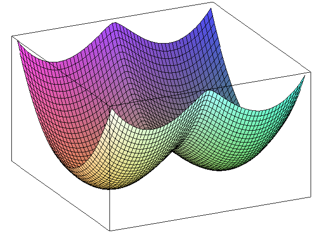
Figure 1. The surface $z=E(u,v)$.

The system (3.1) has three equilibrium points, given by the zeroes of $g(u)$. Namely,

$$0=(0,0)\quad\text{and }\;\;P_{0}^{\pm}=(u_{0}^{\pm},0),\quad\text{for }\;u_{0}^{\pm}=u_{0}^{\pm}(\lambda):=\pm\left(\frac{a}{\lambda}\right)^{\frac{1}{1-p}}.$$

Figure 2 shows the energy level lines of (3.4). Every solution of (3.1) lies on some energy level line.

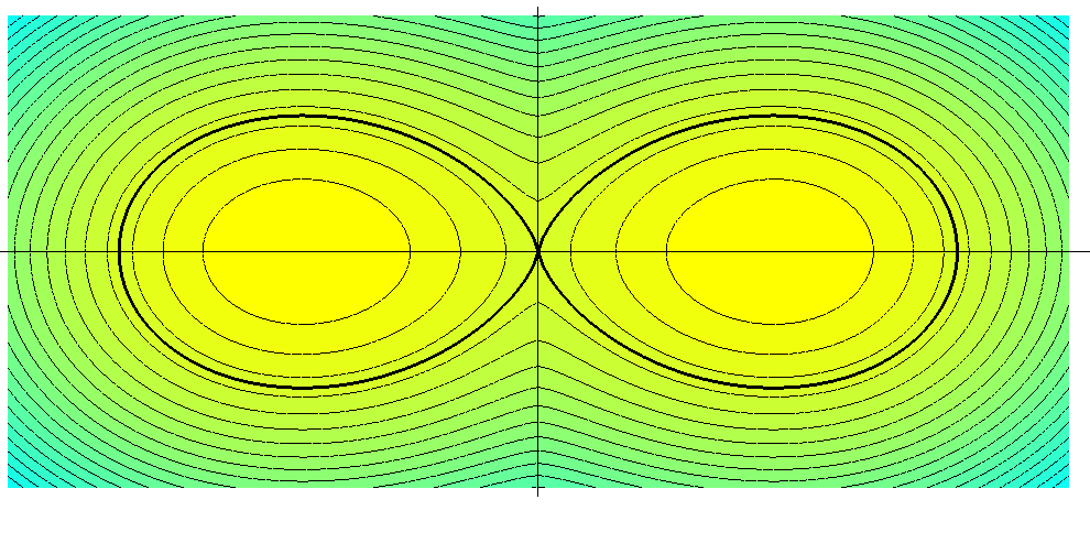
Figure 2. Level lines of the energy function. We have highlighted $[E=0]$.

Next we consider the energy level passing through the origin

$$[E=0]:=\{(u,v)\in{\mathbb{R}}^{2}:\,E(u,v)=0\},$$

which is expressed by the relation $v=\pm\sqrt{-2G(u)}$, where $G(u)$ is the potential energy. By (3.3),

$$\sqrt{-2G(u)}=\left(\frac{2a}{p+1}\right)^{1/2}|u|^{\frac{p+1}{2}}\left(1-\frac{\lambda(p+1)}{2a}|u|^{1-p}\right)^{1/2}.$$ (3.5)

The level set $[E=0]$ splits into 3 pieces:

$$[E=0]=\{(0,0)\}\cup\mathcal{O}^{+}\cup\mathcal{O}^{-},$$

where

$$\mathcal{O}^{+}=\{y=\pm\sqrt{-2G(u)}:\quad 0<u\leq u_{H}\}$$

with

$$u_{H}\equiv u_{H}(\lambda):=\left(\frac{2a}{\lambda(p+1)}\right)^{\frac{1}{1-p}}=\frac{1}{\lambda^{\frac{1}{1-p}}}w_{H},\qquad w_{H}:=\left(\frac{2a}{p+1}\right)^{\frac{1}{1-p}},$$ (3.6)

and $\mathcal{O}^{-}$ is the symmetric of $\mathcal{O}^{+}$ with respect to the $v$-axis. The sets $\mathcal{O}^{+}$ and $\mathcal{O}^{-}$ are homoclinic loops around the equilibrium points $P_{0}^{+}$ and $P_{0}^{-}$, respectively. As will be shown later, these are degenerate homoclinic orbits in the sense that they reach $(0,0)$ in a finite time because of the lack of a Lipschitz condition at $u=0$. This situation is reminiscent of the one studied in [6, Section 2] in the analysis of the equation

$$-u^{\prime\prime}=su^{\beta}-ru^{\alpha}$$

for $r,s>0$ and $0<\alpha<\beta<1$. This equation arises in modeling the Liebau phenomenon in blood circulation (see [39, Ch.8]). The lack of Lipschitz continuity enables the existence of solutions of (1.5) that vanish on some internal subintervals of $(0,L)$ and are otherwise positive in $(0,L)$. It shows that, even in the simplest prototypes of (1.1) one cannot expect the solutions positive in $\Omega$ to satisfy $u>>0$. In particular, the available maximum principle when $p\geq 1$ is lost for all $p\in(0,1)$. Naturally, such pathologies straighten the importance of Theorem 2.1.

The remaining solutions of (1.3) are uniquely determined by their initial conditions and globally defined in time. This follows either by a direct inspection, or using the results of [35], where the problem of the uniqueness for planar Hamiltonian systems without a local Lipschitz condition for the vector field was discussed. Therefore, the system (3.1) defines a dynamical system on the open set $\mathcal{A}={\mathbb{R}}^{2}\setminus[E=0]$. Indeed, for every initial point $P\in\mathcal{A}$, there is a unique solution,

$$z(\cdot;P)=(u(\cdot;P),v(\cdot;P))=(u(\cdot;P),u^{\prime}(\cdot;P)),\qquad z(0;P)=P$$

of the system (3.1), which is globally defined in time. Actually, it is a periodic solution; possibly an equilibrium point if $P=P_{0}^{\pm}$.

Figure 3 shows the graphs of three solutions $(x,u(x))$ of (1.3) with initial points $(u_{H},0),$ $(u_{H}-\varepsilon,0)$ and $(u_{H}+\varepsilon,0)$, for sufficiently small $\varepsilon>0$, where $u_{H}$ is the positive abscissa of the crossing point of the homoclinic $\mathcal{O}^{+}$ with the $u$-axis, given in (3.6). Thus, the solution departing from $(u_{H},0)$ corresponds to the homoclinic loop $\mathcal{O}^{+}$, having $u_{H}$ as its maximum value and vanishing at a finite time $\pm T_{H}$ (the precise value of $T_{H}$ is given in (3.8)). The solution departing from $(u_{H}-\varepsilon,0)$ is periodic and it oscillates around the positive equilibrium point $P_{0}^{+}$, while the solution departing from $(u_{H}+\varepsilon,0)$ is periodic and it oscillates around the origin. This latter solution, truncated on the open interval determined by its first left and right zeros, provides us with a classical positive solution of (1.5), with nonzero first derivative at the boundary points, for the appropriate value of $L>0$ (the distance between the two consecutive zeroes).

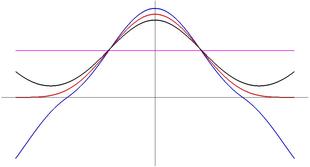
Figure 3. Three solutions of (1.3). The simulation is made for the coefficients $\lambda=1,$ $a=2$ and $p=1/2.$ For the initial point we have taken $u_{H}=64/9$ (according to (3.6)) and $\varepsilon=1/2.$ All these solutions have their first inflection point at level $u=u_{0}^{+}$ (the abscissa of the nontrivial equilibrium point).

Our analysis now proceeds by considering the three different situations illustrated in Figure 3. Since we are interested in non-negative solutions, we will restrict ourselves to the study of the solutions of (3.1) in the half-plane $u\geq 0$. For every $c>u_{H}$, the solution $u(\cdot;c):=u(\cdot;(c,0))$ of (1.3) with initial value $u(0)=c$ such that $u^{\prime}(0)=0$ is positive in a maximal open interval $I_{c}=(-T(c),T(c))$. Moreover, it vanishes with nonzero first derivative at $\pm T(c)$. Thus, these solutions provide us with a positive solution of (1.5) for $L=2T(c)$. In this paper, these strongly positive solutions will be refereed to as classical positive solutions of (1.5). They satisfy $u(x)>0$ for all $x\in(0,L)$, $u^{\prime}(0)>0$ and $u^{\prime}(L)<0$. When some of these conditions fail but $u\not\equiv 0$ the solution will be called degenerate. Thus, if $u$ is a degenerate positive solution, then $u(x_{0})=u^{\prime}(x_{0})=0$ for some $x_{0}\in[0,L]$. Naturally, a degenerate solution might vanish on some, or several, subintervals of $(0.L)$. Such positive solutions are said to be highly degenerate.

If, instead of $c>u_{H}$, we pick $c\in(u_{0}^{+},u_{H})$, then $u(\cdot;c):=u(\cdot;(c,0))$ is a positive periodic solution oscillating around $P_{0}^{+}$, with half-period denoted by $\tau(c)$, such that $\max u=c$ and $\min u=d(c)\in(0,u_{0}^{+})$ with $G(d(c))=G(c)$. Thus, the equilibrium point $P_{0}^{+}$ is a (local) center and $\{(0,0)\}\cup\mathcal{O}^{+}$ is the boundary of the open region around $P_{0}^{+}$ filled in by periodic orbits.

Under these circumstances, since the orbits in $\mathcal{A}$ intersect the $v$-axis and the line $u=u_{0}^{+}$ transversally, the Conley–Wazėwski theory [7] guarantees that the mappings $(u_{H},+\infty)\ni c\mapsto T(c)$ and $(u_{0}^{+},u_{H})\ni c\mapsto\tau(c)$ are continuous (see also [17, pp. 82-84] for the details). However, the fact that

$$\lim_{c\downarrow u_{H}}T(c)=T(u_{H})=T_{H}\quad\hbox{and}\quad\lim_{c\uparrow u_{H}}\tau(c)=T(u_{H})=T_{H}$$

is far from obvious. It will be established later.

As already commented above, the solution of (1.3) with $u(0)=u_{H}$ and $u^{\prime}(0)=0$, which parameterizes the degenerate homoclinic loop $\mathcal{O}^{+}$, reaches the origin in a finite time. A similar situation was discussed in [31] for $-u^{\prime\prime}=-a(x)u^{p}$, with $0<p<1$ and $a(x)$ positive and increasing. More precisely, in [31] the existence of a $\gamma>0$ for which there are solutions of (1.3) with $u(0)=\gamma>0$ and $u^{\prime}(0)=0$ such that $u(\xi^{*})=u^{\prime}(\xi^{*})=0$ for some $\xi^{*}=\xi(\gamma^{*})$ was shown. Some further developments in a similar vain can be found in [3], in studying the non-negative solutions of PDEs with a sign-indefinite weight, and in [5], where solutions with the same property were found in searching for periodic solutions to the second-order equation $-u^{\prime\prime}=a(x)g(u)$ with $g(u)u\geq 0$ and $a(x)$ changing sign, in the “sublinear case” $g(u)/u\to+\infty$ for $u\to 0$. The function $g(u)$ defined in (3.2) does not satisfy these requirements.

3.1. The degenerate homoclinic solution

Consider the solution of (1.3) with $(u(0),u^{\prime}(0))=(u_{H},0)$. As long as $v(x)=u^{\prime}(x)>0$, it follows from $u^{\prime}(x)=\sqrt{-2G(u(x))}$ that the necessary time to reach $u_{2}$ from $u=u_{1}$, with $0<u_{1}<u_{2}<u_{H}$, along $\mathcal{O}^{+}$ in the upper-half plane is given through

$$t(u_{1},u_{2})=\int_{u_{1}}^{u_{2}}\frac{du}{\sqrt{-2G(u)}}.$$

Letting $u_{1}\to 0^{+}$ and $u_{2}\to u_{H}^{-}$, and taking onto account that

$$u_{H}^{1-p}=\frac{2a}{\lambda(p+1)},$$

it follows from (3.5) that the vanishing time from the maximum point $u_{\max}=u_{H}$ to $u=0$ along $\mathcal{O}^{+}$ can be expressed through the convergent improper integral

$$T_{H} \equiv t(0,u_{H})=\int_{0}^{u_{H}}\frac{du}{\sqrt{-2G(u)}}=\left(\frac{2a}{p+1}\right)^{-1/2}\int_{0}^{u_{H}}\frac{du}{u^{\frac{p+1}{2}}\sqrt{1-\frac{\lambda(p+1)}{2a}u^{1-p}}}$$

$$= \lambda^{-1/2}\left(\frac{2a}{\lambda(p+1)}\right)^{-1/2}\int_{0}^{u_{H}}\frac{du}{u^{\frac{p+1}{2}}\sqrt{1-u_{H}^{-(1-p)}u^{1-p}}}$$

$$= \frac{1}{\sqrt{\lambda}}u_{H}^{-\frac{1-p}{2}}\int_{0}^{u_{H}}\frac{du}{u^{\frac{p+1}{2}}\sqrt{1-u_{H}^{-(1-p)}u^{1-p}}}.$$

Thus, the change of variables $u=u_{H}s$, $0<u<u_{H}$, $0<s<1$, leads to

$$T_{H}=\frac{1}{\sqrt{\lambda}}u_{H}^{-\frac{1-p}{2}}\int_{0}^{1}\frac{u_{H}\,ds}{u_{H}^{\frac{p+1}{2}}s^{\frac{p+1}{2}}\sqrt{1-s^{1-p}}}=\frac{1}{\sqrt{\lambda}}\int_{0}^{1}\frac{ds}{s^{\frac{p+1}{2}}\sqrt{1-s^{1-p}}}<\infty.$$ (3.7)

By the symmetry of the problem, $T_{H}$ provides us with the extinction time of the solution of (1.3) such that $u(0)=u_{H}$ and $u^{\prime}(0)=0$. Note that it is independent of the parameter $a$. The expression (3.7) can be further simplified by the new change of variable

$$s^{1-p}=\sin^{2}\theta,\qquad 0<s<1,\quad 0<\theta<\frac{\pi}{2}.$$

Indeed, since $(1-p)s^{-p}=2\sin\theta\cos\theta$, it is clear that

$$T_{H} = \frac{1}{\sqrt{\lambda}}\int_{0}^{1}\frac{ds}{s^{\frac{p+1}{2}}\sqrt{1-s^{1-p}}}=\frac{1}{\sqrt{\lambda}(1-p)}\int_{0}^{1}\frac{(1-p)s^{-p}\,ds}{s^{\frac{p+1}{2}}s^{-p}\sqrt{1-s^{1-p}}}$$

$$= \frac{1}{\sqrt{\lambda}(1-p)}\int_{0}^{1}\frac{(1-p)s^{-p}\,ds}{(s^{1-p})^{1/2}\sqrt{1-s^{1-p}}}=\frac{1}{\sqrt{\lambda}(1-p)}\int_{0}^{\pi/2}\frac{2\sin\theta\cos\theta\,d\theta}{\sin\theta\sqrt{1-\sin^{2}\theta}}.$$

Therefore,

$$T_{H}=T_{H}(\lambda)=\frac{\pi}{\sqrt{\lambda}(1-p)}.$$ (3.8)

Another way to prove (3.8) is to express $T_{H}$ as

$$T_{H}\equiv T_{H}(\lambda)=\frac{1}{\sqrt{\lambda}}\int_{0}^{1}\frac{ds}{s^{\frac{p+1}{2}}\sqrt{1-s^{1-p}}}=\frac{1}{\sqrt{\lambda}}\int_{0}^{1}\frac{ds}{s\sqrt{s^{p-1}-1}}$$ (3.9)

and observe that, up to an additive constant,

$$\int\frac{ds}{s\sqrt{s^{p-1}-1}}=-\frac{2\arctan\sqrt{s^{p-1}-1}}{1-p}.$$ (3.10)

Finally, evaluating the definite integral of (3.9), (3.8) follows readily.

Figure 4 illustrates the independence of the extinction time $T_{H}$ with respect to the coefficient $a$. It plots the graphs $(x,u(x))$ of the degenerate homoclinic solution on the interval $[-T_{H},T_{H}]$ for a given value of $\lambda$ and several choices of the parameter $a$.

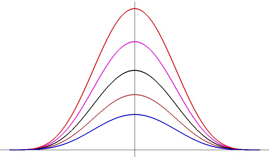
Figure 4. Five solutions of (1.3) having the same extinction time, $T_{H}$, for $(\lambda,p)$ constant and $a$ varying. The simulation has been made with $\lambda=1$ and $p=1/2$. For the initial point we have taken $(u_{H},0)$ (according to (3.6)). The solutions have been computed for the following series of values: $a=1$ ($u_{H}=16/9$), $a=5/4$ ($u_{h}=16/9$), $a=3/2$ ($u_{H}=4$), $a=7/4$ ($u_{H}=49/9$), $a=2$ ($u_{H}=64/9$).

Summarizing, the homoclinic loop $\mathcal{O}^{+}$ degenerates in the sense that the solution of (1.3) with $u(0)=u_{H}$ and $u^{\prime}(0)=0$, denoted by $\hat{u}\equiv\hat{u}_{\lambda}$ in the sequel, runs through the loop in a finite time

$$2T_{H}\equiv 2T_{H}(\lambda)=\frac{2\pi}{\sqrt{\lambda}(1-p)}.$$ (3.11)

This in strong contrast with the classical case of

$$-u^{\prime\prime}=-\lambda u+a|u|^{p-1}u$$

when $p>1$ and which has a similar portrait as in Figure 2, where an infinite amount of time is needed to traverse the loop. Note that $\lim_{p\uparrow 1}T_{H}(\lambda)=\infty$ for all $\lambda>0$. Moreover, according to (3.6),

$$\max\hat{u}_{\lambda}=u_{H}=\frac{1}{\lambda^{\frac{1}{1-p}}}w_{H},\qquad w_{H}:=\left(\frac{2a}{p+1}\right)^{\frac{1}{1-p}}.$$ (3.12)

Since (1.3) is autonomous, any shift in the $x$-variable also provides us with a solution of the equation. Thus, for every $x_{0}\in\mathbb{R}$, $\hat{u}_{\lambda}(\cdot-x_{0})$ is a solution of (1.3) with $u(x_{0})=u_{H}$ and $u^{\prime}(x_{0})=0$, which is unique on the interval

$$[x_{0}-T_{H},x_{0}+T_{H}]={\rm supp\,}\hat{u}_{\lambda}(\cdot-x_{0}).$$

In particular, since

$$\lim_{\lambda\uparrow\infty}T_{H}(\lambda)=0,$$ (3.13)

it follows that for every $x_{0}\in(0,L)$ and $\lambda$ large enough that $0<x_{0}-T_{H}$ and $x_{0}+T_{H}<L$, the extended function

$$\tilde{u}_{\lambda,x_{0}}(x):=\left\{\begin{array}[]{ll}0&\quad\hbox{if}\;\;0\leq x<x_{0}-T_{H},\\ \hat{u}_{\lambda}(x-x_{0})&\quad\hbox{if}\;\;x_{0}-T_{H}\leq x\leq x_{0}+T_{H},\\ 0&\quad\hbox{if}\;\;x_{0}+T_{H}<x\leq L,\end{array}\right.$$ (3.14)

is a positive solution of the nonlinear boundary value problem (1.5), which is highly degenerate. The precise values of $\lambda$ for which this construction can be done will be determined later. Thus, the maximum principle fails for this type of sublinear nonlinearitiy. Note that due to (3.13), for every $x_{0}\in(0,L)$,

$$\lim_{\lambda\uparrow\infty}\left(\lambda^{\frac{1}{1-p}}\tilde{u}_{\lambda,x_{0}}(x)\right)=\left\{\begin{array}[]{ll}0&\quad\hbox{if}\;\;x\in[0,L]\setminus\{x_{0}\},\\ w_{H}=\left(\frac{2a}{p+1}\right)^{\frac{1}{1-p}}&\quad\hbox{if}\;\;x=x_{0}.\end{array}\right.$$ (3.15)

Making the change of variable $v=\lambda^{\frac{1}{1-p}}u$, (1.5) becomes

$$\left\{\begin{array}[]{ll}-\frac{1}{\lambda}\Delta v=v-av^{p}&\quad\hbox{in}\;\;[0,L],\\[4.30554pt] v(0)=v(L)=0,&\end{array}\right.$$ (3.16)

for $\Delta=\frac{d^{2}}{dx^{2}}.$ Then, (3.15) provides us with the limiting behaviour as $\lambda\uparrow\infty$ of the positive solutions of the singular perturbation problem (3.16). Naturally, for every integer $m\geq 1$, and $m$ given points $x_{j}\in(0,L)$, $1\leq j\leq m$, such that

$$(x_{i}-T_{H},x_{i}+T_{H})\cap(x_{j}-T_{H},x_{j}+T_{H})=\emptyset\;\text{if }\;i\not=j,$$ (3.17)

the superposition

$${u}_{\lambda,x_{1},...,x_{m}}(x):=\sum_{j=1}^{m}\tilde{u}_{\lambda,x_{j}}(x),\qquad x\in[0,L],$$ (3.18)

also provides us with a solution of (1.5) due to the assumption (3.17). By (3.13), the solution (3.18) satisfies

$$\lim_{\lambda\uparrow\infty}\left(\lambda^{\frac{1}{1-p}}u_{\lambda,x_{1},...,x_{m}}(x)\right)=\left\{\begin{array}[]{ll}0&\quad\hbox{if}\;\;x\in[0,L]\setminus\{x_{1},...,x_{m}\},\\ w_{H}=\left(\frac{2a}{p+1}\right)^{\frac{1}{1-p}}&\quad\hbox{if}\;\;x\in\{x_{1},...,x_{m}\}.\end{array}\right.$$

Since $[0,L]$ is compact, this construction cannot be done if we choose a countable set of points $x_{j}\in(0,L)$, $j\geq 1$, because the $x_{j}$’s would accumulate at some $x_{0}\in[0,L]$. Thus, (3.17) cannot be satisfied. When dealing with solutions in ${\mathbb{R}}$, a countable number of terms in the sum in (3.18) is allowed provided that the points $x_{j}$, $j\geq 1$, are separated away from each other by a minimal distance. Actually, as the solutions of (1.5) arise in pairs, in the sense that $u$ solves (1.5) if, and only if, $-u$ is also a solution, similar multiplicity results can be given for sign-changing solutions of (1.5). In this case, gluing together positive and negative homoclinic loops, solutions of (1.5) of the form

$${\mathscr{W}}(x)=\sum_{j=1}^{m}\delta_{j}\tilde{u}_{\lambda,x_{j}}(x),\qquad\delta_{j}=\pm 1,$$

can be obtained provided (3.17) holds. Clearly, these degenerate situations are due to the lack of uniqueness for the associated Cauchy problem at the origin. These results should be compared with the gluing of variational solutions found in [28].

Figure 5 shows a family of nested homoclinics for $\lambda$ ranging from a smaller value (the external orbit) to a larger one (the smaller orbit). This displays the dependence of $\max\hat{u}_{\lambda}$ on the parameter $\lambda$.

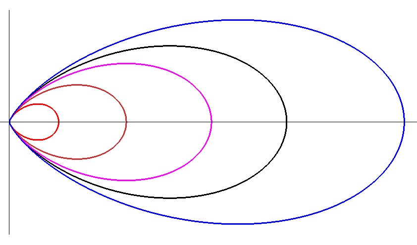
Figure 5. Different atypical homoclinics of system (3.1) for a fixed pair $(a,p)$ and different values of $\lambda$. The simulation is made for the coefficients $a=2$ and $p=2/3.$ The values chosen for $\lambda$ vary from $\lambda=1$ the external orbit) to $\lambda=2$ (the smallest orbit).

We conclude our analysis of these degenerate homoclinics by providing an explicit expression for $\hat{u}_{\lambda}$ as follows. The same argument as in the beginning of Section 3.1 shows that the distance, $|x|$, from $u(x)=u_{1}$ and $u(0)=\max u=u_{H}$ is given by

$$|x|=\int_{u(x)}^{u_{H}}\frac{d\xi}{\sqrt{-2G(\xi)}}.$$

Thus, repeating the same change of variables leading to (3.7), $\xi=u_{H}s$, yields

$$|x|=\frac{1}{\sqrt{\lambda}}\int_{\frac{u(x)}{u_{H}}}^{1}\frac{ds}{s^{\frac{p+1}{2}}\sqrt{1-s^{1-p}}}.$$

Thus it follows from (3.9) and (3.10) that

$$|x|=\frac{2}{(1-p)\sqrt{\lambda}}\arctan\sqrt{\left(\tfrac{u(x)}{u_{H}}\right)^{p-1}-1}$$

and hence,

$$\left(\frac{u(x)}{u_{H}}\right)^{p-1}=1+\tan^{2}\frac{(1-p)\sqrt{\lambda}|x|}{2}.$$

Finally, because of (3.6), we obtain the explicit expression

$$\hat{u}_{\lambda}(x)=\left(\frac{2a}{\lambda(p+1)\left(1+\tan^{2}\frac{(1-p)\sqrt{\lambda}|x|}{2}\right)}\right)^{\frac{1}{1-p}}$$

for every $-T_{H}<x<T_{H}$, $T_{H}=T_{H}(\lambda)$. By construction, $\hat{u}_{\lambda}(x)>0$ for all $x\in(-T_{H},T_{H})$ and

$$\lim_{x\to\pm T_{H}}\hat{u}_{\lambda}(x)=0,\qquad\lim_{x\to\pm T_{H}}\hat{u}^{\prime}_{\lambda}(x)=0.$$ (3.19)

3.2. The classical positive solutions

This section characterizes the existence of strongly positive solutions of (1.5), also referred to as classical positive solutions in this paper. Namely they are solutions satisfying

$$u(x)>0\quad\hbox{for all}\;\;x\in(0,L),\quad u^{\prime}(0)>0,\quad u^{\prime}(L)<0.$$ (3.20)

By the analysis already done in Section 3.1, they are given by the solutions of (1.3) with $u(0)=c$ and $u^{\prime}(0)=0$ for some $c>u_{H}$, and they are defined in some interval $(-T(c),T(c))$ with $u(\pm T(c))=0$, $u^{\prime}(-T(c))>0$, $u^{\prime}(T(c))<0$, $T(c)=L/2$, and $u(x)>0$ for all $x\in(-T(c),T(c))$. In the interval $(-T(c),0)$, where $u(x)>0$ and $u^{\prime}(x)>0$, the solution lies on the energy level $E(u,v)=E(c,0)=G(c)$. From

$$u^{\prime}(x)=\sqrt{2(G(c)-G(u(x)))},$$

as long as $u^{\prime}(x)=v(x)>0$, it is easily seen that the necessary “time” to reach $u=u_{1}\in(0,c)$ from $u=0$ along the orbit in the upper-half plane is given by

$$t(0,u_{1})=\int_{0}^{u_{1}}\frac{du}{\sqrt{2(G(c)-G(u))}}.$$

Thus, letting $u_{1}\uparrow c$ and recalling the definition of $G(u)$, allows us to conclude that the vanishing time $T(c)$ from the maximum point $\max u=c$ to $u=0$ along the level line passing through $(c,0)$ can be expressed via the convergent improper integral

$$T(c)=\int_{0}^{c}\frac{du}{\sqrt{2(G(c)-G(u))}}=\int_{0}^{c}\frac{du}{\sqrt{\lambda(c^{2}-u^{2})-\frac{2a}{p+1}\bigl{(}c^{p+1}-u^{p+1}\bigr{)}}}.$$ (3.21)

(See [27] for similar computations). Performing the change of variables $u=cs$, $0<u<c$, $0<s<1$, it follows from (3.21) that

$$T(c)=\int_{0}^{1}\frac{c\,ds}{\sqrt{\lambda c^{2}(1-s^{2})-\frac{2ac^{p+1}}{p+1}\bigl{(}1-s^{p+1}\bigr{)}}}=\frac{1}{\sqrt{\lambda}}\int_{0}^{1}\frac{ds}{\sqrt{(1-s^{2})-\frac{2a}{\lambda(p+1)}\frac{1}{c^{1-p}}\bigl{(}1-s^{p+1}\bigr{)}}}.$$

This equation together with (3.6) yields

$$T(c)=\frac{1}{\sqrt{\lambda}}\int_{0}^{1}\frac{ds}{\sqrt{(1-s^{2})-\left(\frac{u_{H}}{c}\right)^{1-p}\bigl{(}1-s^{p+1}\bigr{)}}}.$$ (3.22)

Observe that, since $0<p<1$, we have that $1-s^{2}>1-s^{p+1}$ for all $0<s<1$. Therefore the mapping $(u_{H},+\infty)\ni c\mapsto T(c)$ is strictly decreasing. For this particular case, the continuity of $T$ with respect to $c$ also follows directly from (3.22) without having to invoke to any general result on dynamical systems. Note that

$$\lim_{c\uparrow+\infty}T(c)=\frac{1}{\sqrt{\lambda}}\int_{0}^{1}\frac{ds}{\sqrt{1-s^{2}}}=\frac{\pi}{2\sqrt{\lambda}}$$

while, due to (3.7) and (3.8),

$$\lim_{c\downarrow u_{H}^{+}}T(c) =\frac{1}{\sqrt{\lambda}}\int_{0}^{1}\frac{ds}{\sqrt{(1-s^{2})-\bigl{(}1-s^{p+1}\bigr{)}}}$$

$$=\frac{1}{\sqrt{\lambda}}\int_{0}^{1}\frac{ds}{s^{\frac{p+1}{2}}\sqrt{1-s^{1-p}}}=T_{H}=\frac{\pi}{\sqrt{\lambda}(1-p)}.$$

Thus, the map $T(c)$ extends continuously to $[u_{H},+\infty)$ by setting $T(u_{H})=T_{H}$. Figure 6 shows the graph of the mapping $c\mapsto T(c)$. In the light of these facts, it is clear that the boundary value problem (1.5) has a strongly positive solution if, and only if,

$$\lim_{c\uparrow+\infty}T(c)=\frac{\pi}{2\sqrt{\lambda}}<\frac{L}{2}<\frac{\pi}{(1-p)\sqrt{\lambda}}=T_{H}.$$ (3.23)

Moreover, this solution is unique, because there is a unique value of $c>u_{H}$, say $c(\lambda)$, such that $T(c(\lambda))=L/2$. When this occurs, the unique positive solution of (1.5) is given by the $L/2$-shift of the unique positive solution of (1.3) such that $u(L/2)=c(\lambda)$ and $u^{\prime}(L/2)=0$.

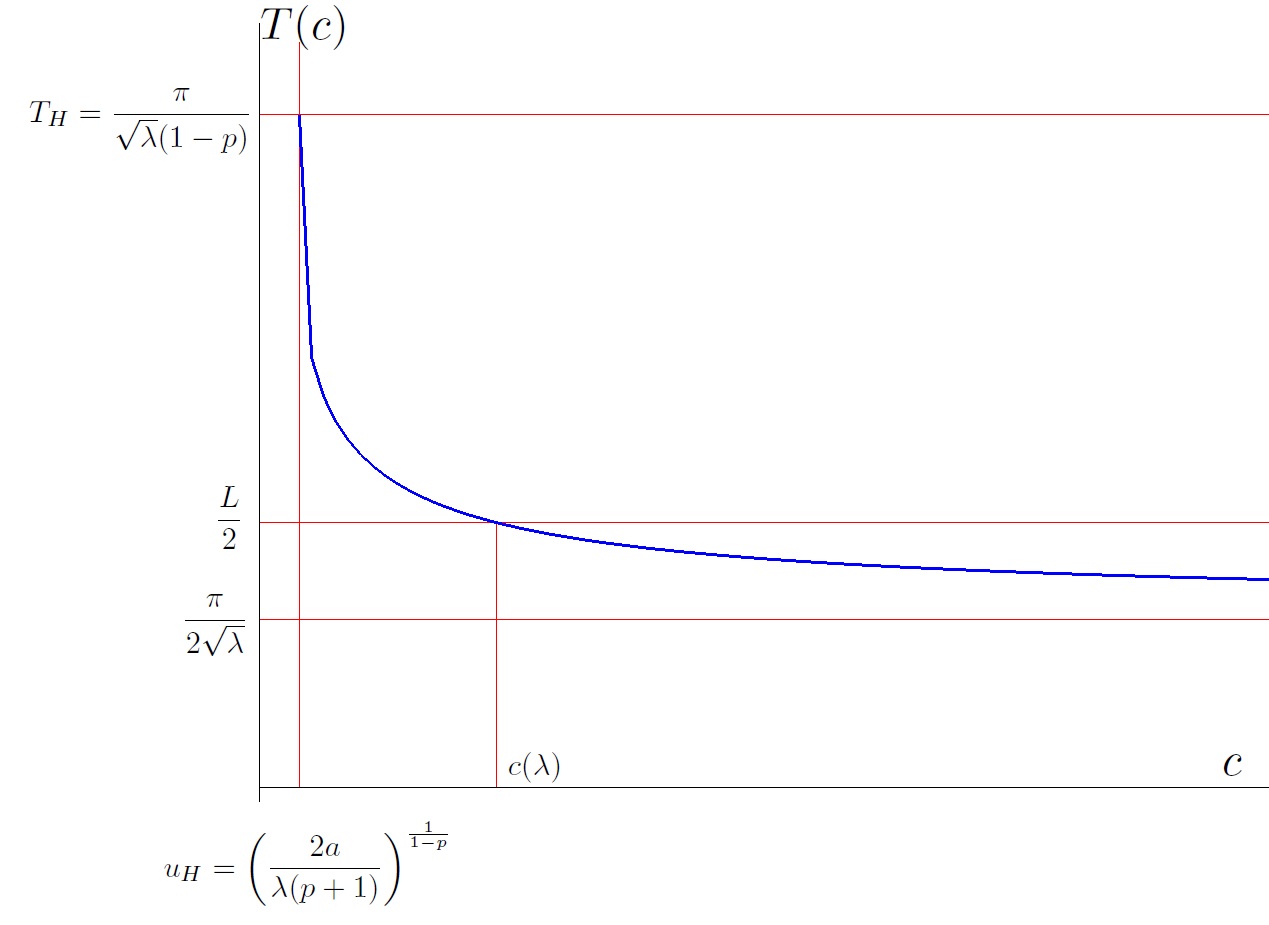
Figure 6. The graph of the time map $T(c)$. It is a decreasing function defined in $[u_{H},\infty)$. By construction, the problem (1.5) has a classical positive solution if, and only if, (3.23) holds. The graph comes from a numerical simulation for the case $a=1,$ $\lambda=1$ and $p=1/2.$

Since (3.23) can be written equivalently as

$$\sigma_{1}=\left(\frac{\pi}{L}\right)^{2}<\lambda<\left(\frac{2}{1-p}\right)^{2}\sigma_{1}\equiv\Sigma_{1}(p),$$ (3.24)

the next result holds.

Theorem 3.1.

The problem (1.5) has a classical positive solution if, and only if, $\lambda\in(\sigma_{1},\Sigma_{1}(p))$, i.e., if (3.24) holds. When (3.24) holds, the solution is unique. Moreover, denoting it by ${u}_{\lambda}$, it satisfies

$$\max{u}_{\lambda}={u}_{\lambda}(L/2)=c(\lambda),$$

and the mapping $(\sigma_{1},\Sigma_{1}(p))\ni\lambda\mapsto c(\lambda)$ is continuous and strictly decreasing with

$$\lim_{\lambda\downarrow\sigma_{1}}c(\lambda)=+\infty,\qquad\lim_{\lambda\uparrow\Sigma_{1}(p)}c(\lambda)=u_{H}(\Sigma_{1}(p))=\left(\frac{2a}{\Sigma_{1}(p)(p+1)}\right)^{\frac{1}{1-p}}.$$ (3.25)

Proof.

We already know that $\lambda\in(\sigma_{1},\Sigma_{1}(p))$ is necessary and sufficient for the existence of a $c(\lambda)>u_{H}$ such that $T(c(\lambda))=L/2$. Moreover, $c(\lambda)$ is unique by the monotonicity of $T(c)$. Thus, the classical positive solution, denoted by $u_{\lambda}$, is unique and it satisfies $u_{\lambda}(L/2)=c(\lambda)$. It also follows from (3.21) that $T(c)$ is a continuous function of $\lambda$. Thus, the definition of $c(\lambda)$ guarantees the continuous dependence of $c(\lambda)$ with respect to $\lambda$.

Next observe that due to (3.21), the identity $T(c)=L/2$ holds for some $c>u_{H}$ if, and only if,

$$\lambda=\Psi(u_{H}/c),$$

where $\Psi$ stands for the map

$$\Psi(\xi):=\left(\frac{2}{L}\right)^{2}\left(\int_{0}^{1}\frac{ds}{\sqrt{(1-s^{2})-\xi^{1-p}\bigl{(}1-s^{p+1}\bigr{)}}}\right)^{2},\qquad 0<\xi<1.$$ (3.26)

From (3.26), since $p<1$, it is easily seen that $\Psi:(0,1)\to\mathbb{R}$ is strictly increasing, with

$$\lim_{\xi\downarrow 0}\Psi(\xi)=\left(\frac{2}{L}\right)^{2}\left(\frac{\pi}{2}\right)^{2}=\left(\frac{\pi}{L}\right)^{2}=\sigma_{1}.$$ (3.27)

Moreover using (3.7) and (3.8), we find that

$$\lim_{\xi\uparrow 1}\Psi(\xi)=\left(\frac{2}{L}\right)^{2}\left(\int_{0}^{1}\frac{ds}{\sqrt{s^{p+1}-s^{2}}}\right)^{2}=\left(\frac{2}{L}\right)^{2}\left(\frac{\pi}{1-p}\right)^{2}=\left(\frac{2}{1-p}\right)^{2}\sigma_{1}=\Sigma_{1}(p).$$ (3.28)

In particular, $\Psi:(0,1)\to\Psi(0,1)=(\sigma_{1},\Sigma_{1}(p))$. Finally, (3.25) follows readily from (3.27) and (3.28). ∎

Note that, since $\lambda\mapsto c(\lambda)$ is continuous, the map $\lambda\mapsto{u}_{\lambda}\in C^{1}_{0}[0,L]$ is also continuous. Moreover, by the uniqueness of $u_{\lambda}$, it follows from (3.25) that in the interval $(\sigma_{1},\Sigma_{1}(p))$, the component $\mathscr{D}^{+}$ whose existence was established by Theorem 2.1 consists of the continuous curve of classical positive solutions defined by

$$\mathscr{C}^{+}:=\{(\lambda,{u}_{\lambda})\;:\;\lambda\in(\sigma_{1},\Sigma_{1}(p))\}.$$

By the construction carried out in Sections 3.1 and 3.2, these classical positive solutions approximate the degenerate solution $\hat{u}$ as $\lambda\uparrow\Sigma_{1}(p)$. Actually, $\hat{u}$ is the unique solution of (1.3) satisfying $u(0)=u_{H}$ and $u^{\prime}(0)=0$. According to (3.19), we already know that $T(u_{H})=L/2$, $\hat{u}(x)>0$ for all $x\in(-L,L)$, $\hat{u}(-L)=\hat{u}(L)=0$, and $\hat{u}^{\prime}(-L)=\hat{u}^{\prime}(L)=0$. Note that $\lambda=K_{1}(p)$ if, and only if, $T_{H}(\lambda)=L/2$. Naturally, since (1.3) is autonomous, the shift

$${u}_{\Sigma_{1}(p)}(x):=\hat{u}\bigl{(}x-\tfrac{L}{2}\bigr{)},\qquad x\in[0,L],$$ (3.29)

provides us with a degenerate positive solution of (1.5). Therefore, in the interval $(\sigma_{1},\Sigma_{1}(p)]$ the component $\mathscr{D}^{+}$ consists of $\mathscr{C}^{+}$ plus the degenerate positive solution $(\Sigma_{1}(p),u_{\Sigma_{1}(p)})$.

3.3. Highly degenerate positive solutions

Next, for every $\lambda>\Sigma_{1}(p)$, we consider the highly degenerate positive solutions $(\lambda,u_{\lambda})$, with

$$u_{\lambda}(x):=\tilde{u}_{\lambda,L/2},$$

where $\tilde{u}_{\lambda,L/2}$ stands for the solution defined in (3.14) with $x_{0}=L/2$. Note that $\lambda>\Sigma_{1}(p)$ if, and only if, $T_{H}<L/2$. By construction, since $\mathscr{D}^{+}$ is connected, $(\lambda,u_{\lambda})\in\mathscr{D}^{+}$ for all $\lambda>\Sigma_{1}(p)$, by the continuity of the map $\lambda\mapsto u_{\lambda}$, $\lambda>\sigma_{1}$. Therefore,

$$\mathscr{C}^{+}:=\{(\lambda,{u}_{\lambda})\;:\;\lambda>\sigma_{1}\}\subset\mathscr{D}^{+}.$$

The solutions on the curve $\mathscr{C}^{+}$ satisfy the following properties:

• $\mathscr{C}^{+}$ is the graph of a continuous curve $\lambda\mapsto{u}_{\lambda}$ which is defined for all $\lambda>\sigma_{1}$;

• the map $\lambda\mapsto\|{u}_{\lambda}\|_{\infty}$ is strictly decreasing, with

  $$\lim_{\lambda\downarrow\sigma_{1}}\|u_{\lambda}\|_{\infty}=+\infty\quad\hbox{and}\quad\lim_{\lambda\uparrow\infty}\|u_{\lambda}\|_{\infty}=0.$$

  Moreover, (3.15) holds.

• ${u}_{\lambda}$ is a classical positive solution of (1.5) if, and only if, $\lambda\in(\sigma_{1},\Sigma_{1}(p))$. Moreover, $\mathscr{C}^{+}=\mathscr{D}^{+}$ in $(\sigma_{1},\Sigma_{1}(p))$.

• At $\lambda=\Sigma_{1}(p)$, ${u}_{\lambda}$ satisfies $u_{\lambda}(x)>0$ for all $x\in(0,L)$, $u_{\lambda}(0)=u_{\lambda}(L)=0$, and $u_{\lambda}^{\prime}(0)=u_{\lambda}^{\prime}(L)=0$. Thus, this solution degenerates.

• For every $\lambda>\Sigma_{1}(p),$ the solution ${u}_{\lambda}$ is symmetric about $x=L/2$ and $\max{u}_{\lambda}={u}_{\lambda}(L/2)$. Moreover,

  $${u}_{\lambda}(x)>0\quad\hbox{for all}\quad x\in(\tfrac{L}{2}-T_{H}(\lambda),\tfrac{L}{2}+T_{H}(\lambda)),$$

  while

  $${u}_{\lambda}\equiv 0\quad\hbox{on}\quad[0,L]\setminus(\tfrac{L}{2}-T_{H}(\lambda),\tfrac{L}{2}+T_{H}(\lambda)).$$

  Figure 7 shows some of those solutions.

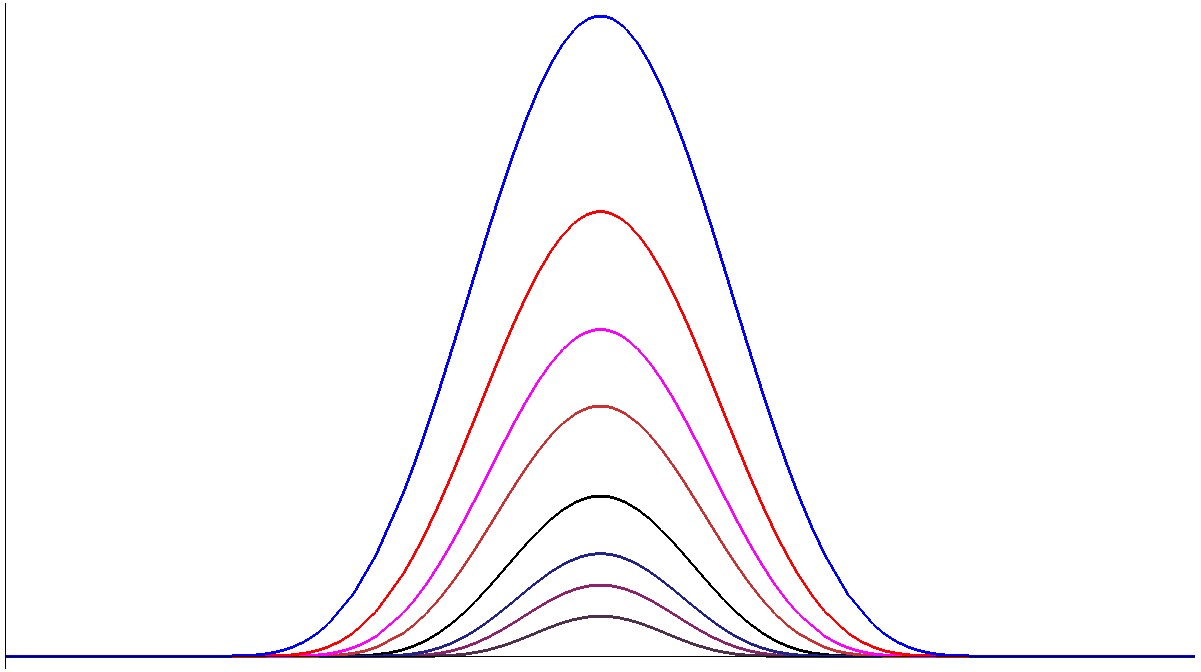
Figure 7. The plots of some highly degenerate solutions of (1.5) for a series of values of $\lambda\in[1,4]$. The solutions decreased as $\lambda$ increased. The numerical experiment has been done with $a=2$ and $p=1/2$. We have taken $L=6\pi>4\pi=2T_{H}(1)$ to guarantee that $u_{\lambda}$ be highly degenerate by choosing $\lambda\geq 1>K_{1}(p)$.

Although $\mathscr{D}^{+}$ consists of a continuous curve on $(\sigma_{1},\Sigma_{1}(p))$, it will be shown that $\mathscr{D}^{+}$ has a more complex structure than $\mathscr{C}^{+}$ for $\lambda>\Sigma_{1}(p)$. Namely, for every $\lambda>\Sigma_{1}(p)$, it contains an additional continuous curve which can be constructed as follows. For every $\lambda>\Sigma_{1}(p)$ and

$$\vartheta\in\left[-\tfrac{L}{2}+T_{H}(\lambda),\tfrac{L}{2}-T_{H}(\lambda)\right],$$

there is a new solution

$${w}_{\lambda,\vartheta}(x):={u}_{\lambda}\bigl{(}x-\vartheta\bigr{)},\quad x\in[0,L].$$

Thus we have a new one-parameter family of highly degenerate solutions of (1.5). Since $\mathscr{D}^{+}$ is connected, and $w_{\lambda,0}=u_{\lambda}\in\mathscr{D}^{+}$, it is clear that

$$w_{\lambda,\vartheta}\in\mathscr{D}^{+}\quad\hbox{for all}\quad\lambda>\Sigma_{1}(p)\quad\hbox{and}\quad\vartheta\in\left[-\tfrac{L}{2}+T_{H}(\lambda),\tfrac{L}{2}-T_{H}(\lambda)\right].$$

Figure 8 shows a few solutions $w_{\lambda,\vartheta}$ for a fixed $\lambda>\Sigma_{1}(p)$ and a series of values of $\vartheta$ varying from $\vartheta^{-}\equiv\vartheta^{-}_{\lambda}:=-\tfrac{L}{2}+T_{H}(\lambda)$ to $\vartheta^{+}\equiv\vartheta^{+}_{\lambda}:=\tfrac{L}{2}-T_{H}(\lambda)$. For $\vartheta=0$, we get the “central”  symmetric solution $w_{\lambda,0}=u_{\lambda}\in\mathscr{C}^{+}\subset\mathscr{D}^{+}$.

By construction, for $\vartheta=\vartheta^{-}$, we have that

$${w}_{\lambda,\vartheta^{-}}(x)={u}_{\lambda}(x-T_{H}),\qquad x\in[0,L].$$

This function satisfies

$${w}_{\lambda,\vartheta^{-}}(0)={w}_{\lambda,\vartheta^{-}}^{\prime}(0)=0,\quad{w}_{\lambda,\vartheta^{-}}(x)>0\;\;\hbox{for all}\;\;x\in(0,2T_{H}),\quad\hbox{and }\;\;{w}_{\lambda,\vartheta^{-}}=0\;\;\hbox{on}\;\;[2T_{H},L].$$

Similarly, for $\vartheta=\vartheta^{+}$, we have that

$${w}_{\lambda,\vartheta^{+}}(x)={w}_{\lambda}(x-L+T_{H}),\qquad x\in[0,L],$$

and this function satisfies

$${w}_{\lambda,\vartheta^{+}}=0\;\;\hbox{on}\;\;[0,L-2T_{H}],\quad{w}_{\lambda,\vartheta^{+}}(x)>0\;\;\hbox{for all}\;\;x\in(L-2T_{H},L),\quad\hbox{and }\;\;{w}_{\lambda,\vartheta^{+}}(L)={w}_{\lambda,\vartheta^{+}}^{\prime}(L)=0.$$

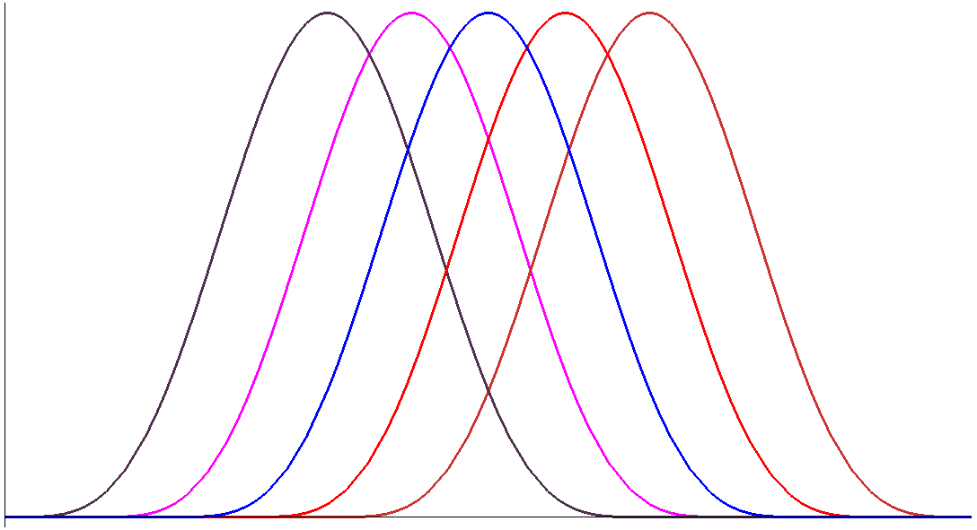
Figure 8. The positive solutions ${w}_{\lambda,\vartheta}$ for a series of values of $\vartheta$ varying from $\vartheta^{-}_{\lambda}$ to $\vartheta^{+}_{\lambda}$. The simulation has been performed with $a=2$, $\lambda=1$, and $p=1/2$. In this case, $2T_{H}(\lambda)=4\pi$. We have taken $L=6\pi>2T_{H}(\lambda)$ so that $\lambda=1>K_{1}(p)$. The figure shows some shifts of the central symmetric solution, $u_{\lambda}$ for some values of the secondary parameter $\vartheta$.

The topological structure of the curve $\mathscr{C}^{+}$ together with the shifted solutions $w_{\lambda,\vartheta}$ for all $\lambda>\Sigma_{1}(p)$ has been sketched in Figure 9. All these solutions are part of the component $\mathscr{D}^{+}$ whose existence was established by Theorem 2.1. Although, for every $\lambda\in(\sigma_{1},\Sigma_{1}(p)]$, $\mathscr{D}^{+}$ consists of $(\lambda,u_{\lambda})$, we see that for every $\lambda>\Sigma_{1}(p)$, the component $\mathscr{D}^{+}$ contains a one-dimensional simplex made by a segment of shifted solutions from $u_{\lambda}$ in the $x$-component. Thus, for every $\lambda>\Sigma_{1}(p)$, (1.5) has a continuum of positive highly degenerate solutions.

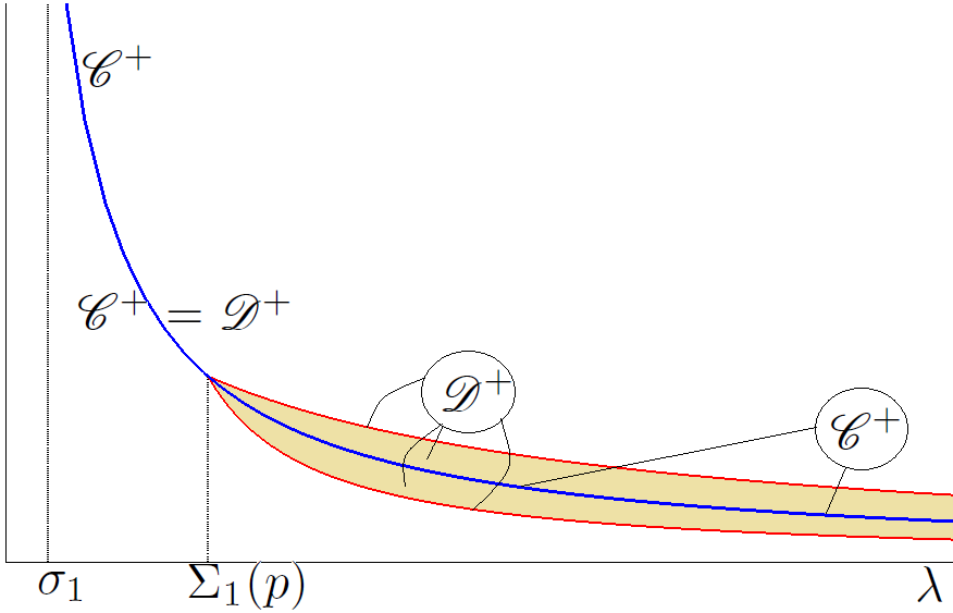
Figure 9. The topological structure of the component $\mathscr{D}^{+}$. It is generated by the central fiber $\mathscr{C}^{+}=\{(\lambda,u_{\lambda})\;:\;\lambda>\sigma_{1}\}$ through the shifts $u_{\lambda,\vartheta}$ for $\lambda>\Sigma_{1}(p)$.

3.4. Multibump solutions

All the solutions constructed in the previous two sections have a single bump in $(0,L)$. In order to complete the classification of the positive solutions of (1.5), both classical and degenerate, we now consider the possibility of solutions with multiple bumps in the interval $[0,L]$. In terms of the dynamics in the phase plane, these solutions can be described as trajectories making multiple transitions of the homoclinic loop $\mathcal{O}^{+}.$ These transitions are separated from each other by periods of “rest” where they remain at the origin. One, or several of these rest intervals might shrink to a single point. Since the time required to complete a homoclinic loop is $2T_{H}(\lambda)$, with $T_{H}(\lambda)$ given by (3.8), $j$ non-overlapping copies of the function ${u}_{\lambda}$ can exist in (0,L) if, and only if,

$$2T_{H}(\lambda)\leq\frac{L}{j}\quad\Leftrightarrow\quad\lambda\geq\Sigma_{j}(p):=\left(\frac{2}{1-p}\right)^{2}\sigma_{j},$$ (3.30)

where $\sigma_{j}:=(j\pi/L)^{2}$ is the $j$-th eigenvalue of $-D^{2}$ in $[0,L]$ under homogeneous Dirichlet boundary conditions. Figure 10 illustrates the case $\lambda=K_{2}(p)$, plotting a solution of (1.5) with two positive humps in $(0,L)$. This solution vanishes with its first derivative at $x\in\{0,L/2,L\}$.

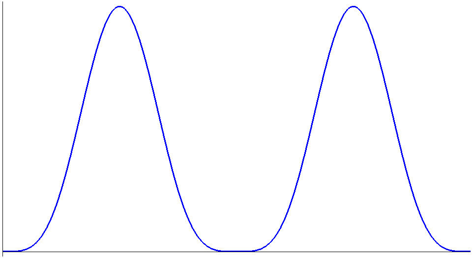
Figure 10. A solution with two bumps computed for the choices $a=2$, $\lambda=1$ and $p=1/2$. We have taken $L=4T_{H}(\lambda)$ so that $\lambda=K_{2}(p)$.

Next the structure of the component of (degenerate) positive solutions with $j\geq 2$ bumps of the problem (1.5) will be described. First, fix $j\geq 2$, suppose $\lambda\geq\Sigma_{j}(\lambda)$, and consider $j$ points

$$0<x_{1}<x_{2}<\cdots<x_{j}<L$$

such that

$$\begin{split}\delta_{1}&:=x_{1}-T_{H}(\lambda)\geq 0,\\ \delta_{i}&:=x_{i}-x_{i-1}-2T_{H}(\lambda)\geq 0\;\;(2\leq i\leq j),\\ \delta_{j+1}&:=L-x_{j}-T_{H}(\lambda)\geq 0,\\ \sum_{i=1}^{j+1}\delta_{i}&=L-2jT_{H}(\lambda).\end{split}$$ (3.31)

Then by construction, the function

$${u}_{\lambda,x_{1},\dots,x_{j}}(x)=\sum_{i=1}^{j}\tilde{u}_{\lambda,x_{i}}(x),\qquad x\in[0,L],$$ (3.32)

provides us with a degenerate positive solution of (1.5) having a bump at each of the points $x_{j}$. In (3.32), $\tilde{u}_{\lambda,x_{i}}$ is the degenerate positive solution defined in (3.14), with $x_{0}=x_{i}$.

The following result shows that, at any of these bumps, the positive solution reaches

$$u_{H}(\lambda)\equiv\left(\frac{2a}{(p+1)\lambda}\right)^{\frac{1}{1-p}}.$$

The proof is omitted, since it is a direct consequence of the analysis previously performed on the homoclinic loops and it also comes from formula (3.6).

Lemma 3.1.

Suppose $0\leq\alpha<\beta\leq L$ and $u$ is a positive solution of

$$\left\{\begin{array}[]{l}-u^{\prime\prime}=\lambda u-a|u|^{p-1}u\quad\hbox{in }[\alpha,\beta],\\ u(\alpha)=u(\beta)=0,\end{array}\right.$$

such that $u(x)>0$ for all $x\in(\alpha,\beta)$. Then,

$$\|u\|_{\infty,[\alpha,\beta]}=u(\tfrac{\alpha+\beta}{2})\geq\left(\tfrac{2a}{(p+1)\lambda}\right)^{\frac{1}{1-p}}$$

As a byproduct, for every $i,j\geq 1$ with $i\neq j$, the components of solutions with $i$ bumps cannot touch any of the components with $j$ bumps. Actually, adapting the argument of Section 3.3, for every $j\geq 2$ and $\lambda>\Sigma_{j}(p)$ (fixed), one can construct from $u_{\lambda,x_{1},...,x_{j}}$ a $j$–dimensional simplex consisting of homotopic solutions to $u_{\lambda,x_{1},...,x_{j}}$ by slightly changing some, or several, of the points $x_{i}$, $1\leq i\leq j$. The underlying simplex of solutions for a given $\lambda>\Sigma_{j}(p)$ expands as $\lambda$ increases, as sketched in Figure 11, where, for evey $j\geq 2$, we have denoted by $\mathscr{D}_{j}^{+}$ the component of highly degenerate positive solutions of (1.5) with $j$ bumps in $(0,L)$. By the construction, it is easily seen that, necessarily, $\mathscr{D}^{+}_{j}$ is the unique component of positive solutions with $j$ bumps, since any pair of solutions of this type are homotopic.

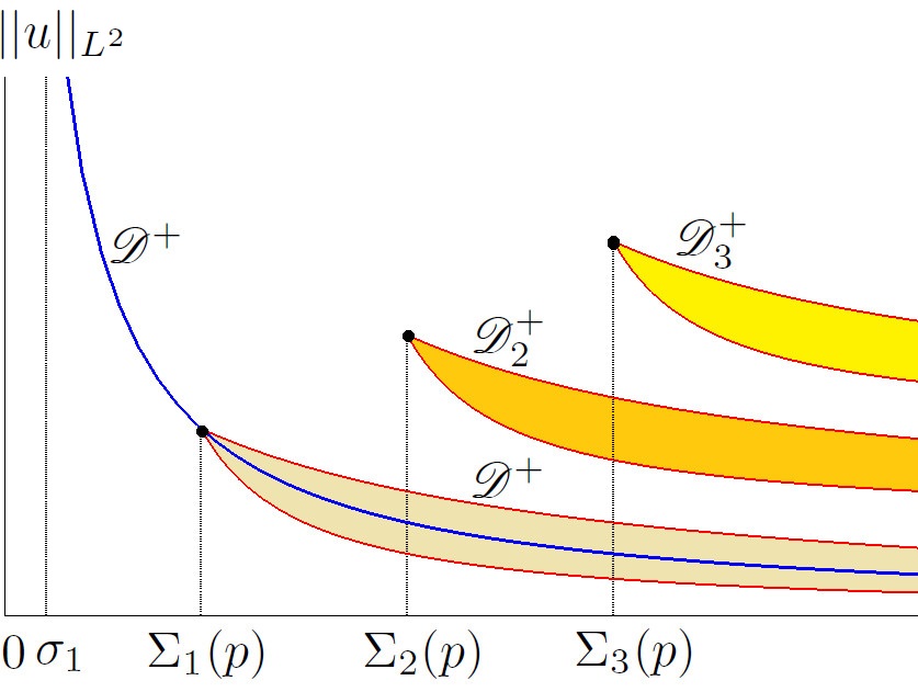
Figure 11. The components of positive solutions with $j\geq 1$ bumps, $\mathscr{D}_{j}^{+}$. We are denoting $\mathscr{D}_{1}^{+}\equiv\mathscr{D}^{+}$.

4. Final comments

The discussion of Section 3 shows that even in the simplest case of (1.5), the problem (1.1) can have multiple degenerate positive solutions for sufficiently large $\lambda$. Actually, in the context of the problem (1.5), for each integer $j\geq 1$ and every $\lambda>\Sigma_{j}(p)$, the problem (1.5) possesses a $\kappa$-simplex of positive solutions with $\kappa$ bumps for all $\kappa\in\{1,...,j\}$, although the component $\mathscr{D}^{+}\equiv\mathscr{D}_{1}^{+}$ constructed in Theorem 2.1 consists of solutions with a single bump.

The fact that ${u}_{\Sigma_{1}(p)}$ vanishes with its first derivatives at the boundary of its domain, allows us to extend it periodically to the whole real line. Moreover, gluing together copies of ${u}_{\Sigma_{1}(p)}$ with the null function, we can also construct positive subharmonic solutions of any order. Actually, the following result concerning “chaotic solutions”  holds.

Theorem 4.1.

Assume $L=2T_{H}(\Sigma_{1}(p))$. Then, given any doubly infinite sequence of symbols $\mathbf{s}=(s_{i})_{i\in\mathbb{Z}}\in\{0,1\}^{\mathbb{Z}},$ there exists a solution $u=u_{\mathbf{s}}$ of (1.5) with the following properties:

• $u\geq 0$ and $\max u=u_{H}(K_{1}(p))$ if $u\neq 0$. Moreover, $u(iL)=u^{\prime}(iL)=0$ for all $i\in\mathbb{Z}$;

• $u|_{((i-1)L,iL)}\equiv 0$ if $s_{i}=0$, while $u(x)>0$ for all $x\in((i-1)L,iL)$ if $s_{i}=1$;

• $u=u_{\mathbf{s}}$ is a subharmonic solution of order $\kappa$ if the sequence $\mathbf{s}$ is $\kappa$-periodic (of minimal period $\kappa$).

Proof.

Given any sequence of two symbols $\mathbf{s}=(s_{i})_{i\in\mathbb{Z}}\in\{0,1\}^{\mathbb{Z}}$, a solution $u=u_{\mathbf{s}}$ can be constructed by gluing together the null solutions in the intervals $[(i-1)L,iL]$ if $s_{i}=0$ and the solution

$$\hat{u}(x-(i-1)L-T_{H}(\Sigma_{1}(p)))=\hat{u}(x-(i-1)L-\tfrac{L}{2}),\quad\text{if }\;(i-1)L\leq x\leq iL,$$

if $s_{i}=1$. Then, it is straightforward to check that all the assertions of the Theorem hold. ∎

The dynamical interpretation of the result is that in the phase plane $(u,u^{\prime})$, we have a trajectory which makes one loop following $\mathcal{O}^{+}$ in the time-interval $((i-1)L,iL)$ when $s_{i}=1,$ while the solution remains at the origin in the time-interval $((i-1)L,iL)$, when $s_{i}=0$. In any case, the solution is at the origin at the times $x=iL$ for all $i\in\mathbb{Z}.$

The same result holds if $L>2T_{H}(\Sigma_{1}(p))$, but then, although

$$\max u|_{((i-1)L,iL)}=u_{H}(\Sigma_{1}(p))>0\quad\hbox{if}\;\;s_{i}=1,$$

the solution $u=u_{\mathbf{s}}$ might vanish on some points inside the interval $((i-1)L,iL)$.

To add more complexity, one can consider chaotic dynamics on three symbols $\{-1,0,1\}$ with a solution, which, in addition to the above described dynamics, also traverses a loop along the degenerate homoclinic $\mathcal{O}^{-}$ during the interval $((i-1)L,iL)$ when $s_{i}=-1$.

The dynamics described in Theorem 4.1 represents an example of chaos in the coin-tossing sense as described in [20]. By that we mean for any given sequence of ${\rm Heads}=0$ and ${\rm Tails}=1,$ a solution can be constructed with the same associated coding (as in in $(b)$ of Theorem 4.1). Such behavior does not seem to fit into the typical definitions of chaotic dynamics in the literature [9, 15]. Indeed most definitions in the literature consider the iterates of a given single-valued continuous map that is often a homeomorphism. However in our situation, the Poincaré map associated with the solutions of system (3.1) is not single-valued in the whole plane due to the lack of uniqueness of the Cauchy problem associated to (3.1). A similar case of “chaos”  for scalar first order differential equations without uniqueness $u^{\prime}=f(t,u)$ was considered in [29]. Later, it was established in [32] that, in spite of the lack of uniqueness of the associated Cauchy problem, there is a way to enter into the classical definitions of chaotic dynamics by defining a suitable subsystem of the Bebutov flow (for the basic theory about the Bebutov flows, see [36, 37]).

Following a similar approach as in [32], we can show that Theorem 4.1 provides indeed a true form of chaotic dynamics if properly interpreted. To this end, we proceed as follows. First of all we introduce the set

$$\mathscr{M}=\{u_{\mathbf{s}}:\,\mathbf{s}=(s_{i})_{i\in\mathbb{Z}}\in\{0,1\}^{\mathbb{Z}}\}$$

of all the solutions $u_{\mathbf{s}}$ of Theorem 4.1. The projection map

$$\Pi:\mathscr{M}\to\{0,1\}^{\mathbb{Z}},\qquad\Pi(u_{\mathbf{s}})=\mathbf{s},$$

is a bijection. Actually, it is a homeomorphism if we take on $\mathscr{M}$ the topology of uniform convergence on compact sets and on $\{0,1\}^{\mathbb{Z}}$ the standard product topology. Now, the $L$-translation on the $x$-component $\Phi_{L}:\mathscr{M}\to\mathscr{M}$ defined by $\Phi_{L}:u(\cdot)\mapsto u(\cdot+L),$ is conjugate with the shift automorphism (also called Bernoulli shift)

$$\vartheta:\{0,1\}^{\mathbb{Z}}\to\{0,1\}^{\mathbb{Z}},\qquad\vartheta:(s_{i})_{i\in{\mathbb{Z}}}\mapsto(s_{i+1})_{i\in{\mathbb{Z}}}.$$

In other words,

$$\Pi\circ\Phi_{L}=\vartheta\circ\Pi.$$

This means that $\Phi_{L}$ on $\mathscr{M}$ has all the dynamical properties of $\vartheta$ on $\{0,1\}^{\mathbb{Z}}.$ Conjugation with the shift map on the set of sequence of $m\geq 2$ symbols is the best known form of “chaos” as it fulfills all the typical features (such as transitivity, density of periodic points, sensitive dependence on initial conditions, positive topological entropy) usually associated with the concept of chaotic dynamics (see [9, 15] for the main definitions and concepts, as well as [38, Section I.5] in the classical work of Smale).

Symbolics dynamics results have also been obtained for more general settings using gluing arguments from the calculus of variations. See, e.g., the survey paper [28] and the references therein. For such gluing arguments, the heads and tails are replaced by a collection of basic solutions of the equations. Each formal concatenation of a collection of basic solutions that makes sense geometrically then corresponds to a nearby actual solution of the equation that is obtained variationally. The nonuniqueness in the current problem replaces the variational arguments by simple direct concatenation, e.g., we get a $2$ bump solution by gluing $2$ one bump solutions that are suitably separated.

References

[1] H. Amann, On the existence of positive solutions of nonlinear elliptic boundary value problems, Indiana Univ. Math. J.21 (1972), 125–146.
[2] A. Ambrosetti and P. H. Rabinowitz, Dual variational methods in critical point theory and applications, J. Funct. Anal.14 (1973), 349–381.
[3] C. Bandle, M. A. Pozio and A. Tesei, The asymptotic behavior of the solutions of degenerate
parabolic equations, Trans. Amer. Math. Soc.303 (1987), 487–501.
[4] H. Berestycki and P. L. Lions, Some applications of the method of super and subsolutions.
Bifurcation and nonlinear eigenvalue problems (Proc., Session, Univ. Paris XIII, Villetaneuse, 1978), pp. 16-41, Lecture Notes in Mathematics 782, Springer, Berlin, 1980.
[5] G. J. Butler, Periodic solutions of sublinear second order differential equations,
J. Math. Anal. Appl.62 (1978), 676–690.
[6] J. A. Cid and L. Sánchez, Nonnegative oscillations for a class of differential equations
without uniqueness: a variational approach, Discrete Contin. Dyn. Syst. Ser. B25 (2020), 545–554.
[7] C. Conley, Isolated Invariant Sets and the Morse Index,
in: CBMS Regional Conference Series in Mathematics, Vol. 38,
American Mathematical Society, Providence, RI, 1978.
[8] M. G. Crandall and P. H. Rabinowitz, Bifurcation from simple eigenvalues, J. Funct. Anal.8 (1971), 321–340.
[9]
R.L. Devaney,
An introduction to chaotic dynamical systems (Second edition),
Addison-Wesley Publishing Company,
Redwood City, CA, 1989.
[10] C. Faber, Beweis das unter allen homogenen Membranen von gleicher Fläche und und gleicher Spannung die
kreisdörmige den tiefsten Grundton gibt, Zitzungsberg. Bayer. Acad. der Wiss. Math. Phys.
(1923), 169–171.
[11] M. Fukuhara, Sur les systémes des équations differentielles ordinaires,
Proc. Imp. Acad. Japan4 (1928), 448–449.
[12] M. Fukuhara and M. Nagumo, Un théorèeme relatif a l’ensemble des curves
intégrales d’un systéeme d´equations différentielles ordinaires, Proc. Phys.
Math. Soc. Japan12 (1930), 233–239.
[13] J. E. Furter and J. López-Gómez, Diffusion-mediated permanence problem for a
heterogeneous Lotka-Volterra competition model, Proc. Roy. Soc. Edinburgh127A
(1997), 281–336.
[14] D. Gilbarg and N. E. Trudinger, Elliptic Partial Differential Equations
of Second Order, Springer, Berlin 2001.
[15]
N. Hasselblatt and A. Katok,
A first course in dynamics. With a panorama of recent developments,
Cambridge University Press, New York, 2003.
[16] P. Hartman, Ordinary Differential Equations, John Wiley and Sons, New
York, 1964.
[17] M. Henrard and F. Zanolin,
Bifurcation from a periodic orbit in perturbed planar Hamiltonian systems,
J. Math. Anal. Appl.277 (2003), 79–103.
[18] U. Kaufmann, H. Ramos Quoirin and K. Umezu, Positivity results for indefinite
sublinear elliptic problems via a continuity argument, J. Diff. Eqns.263 (2017), 4481–4502.
[19] U. Kaufmann, H. Ramos Quoirin and K. Umezu, Uniqueness and positivity issues in a quasilinear
indefinite problem, Cal. Var. (2021), 60:187.
[20]
U. Kirchgraber and D. Stoffer,
On the definition of chaos,
Z. Angew. Math. Mech.69 (1989), 175–185.
[21] H. Kneser, Ueber die Lösungen eines Systems gewöhnlicher Differentialgleichungen
das der Lipschitzschen Bedingung nicht genügt, Preuss. Akad. Wiss. Phys. Math Kl.II4 (1923), 171–174.
[22] E. Krahn, Über eine von Rayleigh formulierte Minimaleigenschaft des Kreises, Math. Ann.91 (1925), 97–100.
[23] J. López-Gómez, The maximum principle and the existence of principal eigenvalues for some linear weighted boundary value problems, J. Differential Equations127 (1996), 263-294.
[24] J. López-Gómez, Spectral Theory and Nonlinear Functional Analysis,
Chapman & Hall/CRC Research Notes in Mathematics 426, Boca Raton, 2001.
[25] J. López-Gómez, Linear Second Order Elliptic Operators, World Scientific, Singapore, 2013.
[26] J. López-Gómez, Metasolutions of Parabolic Equations in Population Dynamics,
CRC Press, Boca Raton, 2015.
[27] J. López-Gómez, E. Muñoz-Hernández and F. Zanolin, Rich dynamics in planar systems with heterogeneous nonnegative weights, Comm. Pure Appl. Anal. (2023), doi:10.3934/cpaa.2023020
[28] P. Montecchiari and P.H. Rabinowitz, A variant of the mountain pass theorem and variational gluing,
Milan J. Math.88 (2020), 347–372.
[29] F. Obersnel and P. Omari,
Period two implies chaos for a class of ODEs,
Proc. Amer. Math. Soc.135 (2007), 2055–2058.
[30] A. Pazy and P. H. Rabinowitz, A nonlinear integral equation with applications to neutron
transport theory, Arch. Rational Mech. Anal.32 (1969), 226–246.
[31] L.A. Peletier and A. Tesei, Global bifurcation and attractivity of stationary solutions
of a degenerate diffusion equation, Adv. in Appl. Math.7 (1986), 435–454.
[32] M. Pireddu,
Period two implies chaos for a class of ODEs: a dynamical system approach,
Rend. Istit. Mat. Univ. Trieste41 (2009), 43–54 (2010).
[33] P. H. Rabinowitz, Some global results for nonlinear eigenvalue problems,
J. Functional Anal.7 (1971), 487–513.
[34] P. H. Rabinowitz, On bifurcation from infinity, J. Differential Eqns.14 (1973), 462–475.
[35] C. Rebelo, A note on uniqueness of Cauchy problems associated to planar Hamiltonian systems,
Portugal. Math.57 (2000), 415–419.
[36] G.R. Sell,
Topological dynamics and ordinary differential equations,
Van Nostrand Reinhold Mathematical Studies, No. 33 Van Nostrand Reinhold Co.,
London, 1971.
[37]
K.S. Sibirsky,
Introduction to topological dynamics
(Translated from the Russian by Leo F. Boron),
Noordhoff International Publishing, Leiden, 1975.