SUBSAMPLING FOR BIG DATA LINEAR MODELS

WITH MEASUREMENT ERRORS

Jiangshan Ju, Mingqiu Wang and Shengli Zhao

School of Statistics and Data Science, Qufu Normal University

Abstract: Subsampling algorithms for various parametric regression models with massive data have been extensively investigated in recent years. However, all existing studies on subsampling heavily rely on clean massive data. In practical applications, the observed covariates may suffer from inaccuracies due to measurement errors. To address the challenge of large datasets with measurement errors, this study explores two subsampling algorithms based on the corrected likelihood approach: the optimal subsampling algorithm utilizing inverse probability weighting and the perturbation subsampling algorithm employing random weighting assuming a perfectly known distribution. Theoretical properties for both algorithms are provided. Numerical simulations and two real-world examples demonstrate the effectiveness of these proposed methods compared to other uncorrected algorithms.

Key words and phrases: Corrected likelihood method, Measurement error, Subsampling algorithm.

1 Introduction

To address the ever-increasing volume of data brought about by technological advancements, it is imperative to adopt refined techniques such as divide and conquer, online updating of streaming data, and subsampling-based methods. These techniques offer effective solutions to computational challenges posed by large datasets. However, existing literature often assumes that direct and accurate observation of covariates, which may not always be feasible in practical data collection scenarios. Consequently, statistical models that do not account for measurement errors can lead to biased estimated results. Therefore, it is essential to investigate subsampling algorithms for linear models that consider measurement errors in covariates.

For the subsampling algorithm of linear models, Ma, Mahoney and Yu (2015) proposed a leverage sampling algorithm based on leverage scores and their linear transformations. A deterministic subsampling method named information-based optimal subdata selection (IBOSS) was proposed by Wang, Yang and Stufken (2019), and extended by Wang (2019b), aiming to find subsamples with the maximum information matrix under the D-optimality criterion, which performs well in finding corners. Cheng, Wang and Yang (2020) and Yu, Liu and Wang (2023) extended the IBOSS algorithm to logistic and nonlinear models, respectively. Wang et al. (2021) proposed an orthogonal subsampling approach for big data linear regression. Yi and Zhou (2023) and Zhang et al. (2024) explored using space-filling or uniform designs to obtain the subsample so that a wide range of models could be considered.

Wang, Zhu and Ma (2018) proposed the optimal subsampling method based on the A-optimality criterion. This method was further developed by Wang (2019a), Ai et al. (2021a), Ai et al. (2021b), Wang and Ma (2021), and Yu et al. (2022). In addition to the widely used method based on inverse probability weighting, Wang and Kim (2022) introduced the maximum sample conditional likelihood estimation, and enhanced the estimator for selected subsamples. This approach overcomes the limitations of inverse probability weighting and makes more efficient use of sample information. Yao and Jin (2024) introduced a perturbation subsampling method that employs repeated random weighting of known distributions to address the limitations of inverse probability weighting. This method has been successfully applied to linear models, longitudinal data, and high-dimensional data with promising performance.

For the measurement error model, Fuller (1987) systematically introduced a comprehensive statistical inference of linear regression models with measurement errors. Nakamura (1990) proposed the corrected score method for the generalized linear model with measurement errors. Carroll et al. (2006) systematically studied the theory of nonlinear regression models with measurement errors. Liang, Hardle and Carroll (1999) offered the parameter estimation of a semi-parametric partially linear model with measurement errors. Liang and Li (2009) examined variable selection in partially linear models with measurement errors, and proposed that when the variance of the measurement error is unknown, it can be estimated through repeated observations. Lee, Wang and Schifano (2020) introduced an online update method for correcting measurement errors in big data streams.

This study focuses on the subsampling problem in linear models with measurement errors. The presence of measurement errors in covariates can introduce inaccuracies of parameter estimation, thereby diminishing the statistical power. We employ the corrected likelihood approach proposed by Nakamura (1990) to estimate the parameters with subsamples. We introduce an optimal subsampling method based on the corrected likelihood approach, and the optimal subsampling probabilities are determined by minimizing the trace of the variance. The consistency and asymptotic normality of estimators obtained by this approach are established. Furthermore, we propose a perturbation subsampling method based on the corrected likelihood approach that approximates the objective function of the full data using a perturbation with independently generated stochastic weights. The effectiveness of our method is also confirmed through numerical analysis. By accounting for measurement errors in covariates, more precise and reliable results can be obtained in the analysis of massive datasets. Our approaches not only alleviate the computational burden associated with parameter estimation in big data but also enhance computational efficiency and improve prediction accuracy.

The rest of the paper is outlined as follows. Section 2 offers a comprehensive introduction to the model setup and parameter estimation of the measurement error model. Sections 3 and 4 introduce the linear model subsampling algorithm with measurement errors and establish the correspondingly theoretical properties. Section 5 comprises numerical simulations. Section 6 presents case studies aimed at validating effectiveness of the algorithm. Finally, Section 7 summarizes this paper. The detailed proofs are provided in the supplementary materials

2 Linear model with measurement errors

In this section, we present an overview of the model and parameter estimation.

2.1 Model

Here, we consider the linear model with measurement errors

$$\left\{\begin{aligned} y_{i}=\mathbf{X}_{i}^{T}\boldsymbol{\beta}+\epsilon_{i}\\ \mathbf{W}_{i}=\mathbf{X}_{i}+\mathbf{U}_{i}\end{aligned}\right.,i=1,2,\ldots,n,$$ (2.1)

where $\mathbf{X}_{i}=(x_{i1},\ldots,x_{ip})^{T}$ is a $p$-dimensional covariate vector, $y_{i}$ is the corresponding response variable, $\boldsymbol{\beta}=(\beta_{1},\beta_{2},\ldots,\beta_{p})^{T}$ is an unknown parameter vector, and $\epsilon_{i}$ is a random error term with mean zero and variance $\sigma^{2}$. However, in applications, the exact value of $\mathbf{X}_{i}$ is often difficult to obtain. Let $\mathbf{U}_{i}=(u_{i1},\ldots,u_{ip})^{T}$ be a random error vector with mean zero and variance-covariance matrix $\boldsymbol{\Sigma}_{uu}$, and $\mathbf{W}_{i}$ be the actual observed random variable. Assuming $\boldsymbol{\Sigma}_{uu}$ is known, the measurement error $\mathbf{U}_{i}$ is independent of $\epsilon_{i}$ and $\mathbf{X}_{i}$.

According to Fuller (1987), the ordinary least squares method cannot be directly applied to estimate linear models with measurement errors, as the resulting estimators are biased and inconsistent. For model (2.1), it follows that

$$y_{i}=\mathbf{W}_{i}^{T}\boldsymbol{\beta}+\epsilon_{i}-\mathbf{U}_{i}^{T}\boldsymbol{\beta}\triangleq\mathbf{W}_{i}^{T}\boldsymbol{\beta}+\delta_{i},~{}i=1,2,\ldots,n,$$

where $\delta_{i}=\epsilon_{i}-\mathbf{U}_{i}^{T}\boldsymbol{\beta}$. Note that

$$Cov(\mathbf{W}_{i},\delta_{i})=Cov(\mathbf{X}_{i}+\mathbf{U}_{i},\epsilon_{i}-\mathbf{U}_{i}^{T}\boldsymbol{\beta})=-\boldsymbol{\Sigma}_{uu}\boldsymbol{\beta}\neq 0.$$

Since the assumption of independence is violated, the ordinary method cannot be applied directly. This also suggests that when there are no measurement errors, i.e., $\boldsymbol{\Sigma}_{uu}=0$, the estimator is unbiased. Example 1 illustrates the influences of measurement errors.

Example 1.

The responses $y_{i}$ are generated from $y_{i}=0.5+0.5x_{i}+\varepsilon_{i}$, $x_{i}\sim N(0,1)$ and $\varepsilon_{i}\sim N(0,1)$, $i=1,\ldots,1000$. We consider the measurement error of the covariate $x_{i}$ by replacing $w_{i}$ with $w_{i}=x_{i}+u_{i}$, $u_{i}\sim N(0,0.5^{2})$. The black solid line represents true model. The blue dotted line represents the regression line fitted by the full dataset, while the red dashed line represents the regression line fitted by a subsample with size 50 selected using L-optimal subsampling. From Figure 1, we can see that the presence of measurement errors in covariates have great effect on the resulting subsample estimator, if measurement errors are ignored.

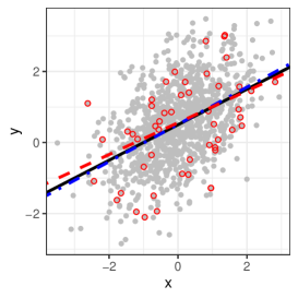
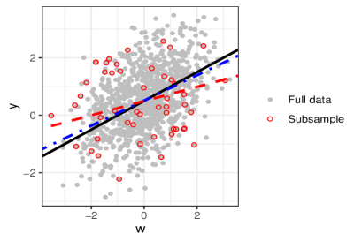
Figure 1: The plot on the left is the fitting result of the data without measurement errors. The plot on the right is the fitting result of the data with measurement errors, while ignoring measurement errors.

2.2 Parameter estimation

To correct measurement errors, we apply the corrected likelihood method proposed by Nakamura (1990). When $\boldsymbol{\Sigma}_{uu}$ is known, using the corrected likelihood method, we obtain

$$\ell(\boldsymbol{\beta})=\frac{1}{2n}\sum_{i=1}^{n}(y_{i}-\mathbf{W}_{i}\boldsymbol{\beta})^{2}-\frac{1}{2}\boldsymbol{\beta}^{T}\boldsymbol{\Sigma}_{uu}\boldsymbol{\beta}.$$

Minimizing $\ell(\boldsymbol{\beta})$, we have

$$\hat{\boldsymbol{\beta}}=\arg\underset{\boldsymbol{\beta}}{\min}\ell(\boldsymbol{\beta})=\left(\sum_{i=1}^{n}\mathbf{W}_{i}\mathbf{W}_{i}^{T}-n\boldsymbol{\Sigma}_{uu}\right)^{-1}\sum_{i=1}^{n}\mathbf{W}_{i}y_{i}.$$

According to Liang, Hardle and Carroll (1999), under certain assumptions, the parameter estimators possess both consistency and asymptotic normality.

Lemma 1.

Suppose that there exists an $s>2$ such that $E\|\mathbf{X}_{i}\|^{2s}<\infty$, $E\|\mathbf{U}_{i}\|^{2s}<\infty$ and $E|\epsilon_{i}|^{2s}<\infty$, where $\|\cdot\|$ represents an Euclidean norm. Additionally, $\frac{1}{n}\sum_{i=1}^{n}\mathbf{X}_{i}\mathbf{X}_{i}^{T}$ converges to the covariance matrix $\mathcal{H}$, where $\mathcal{H}$ is a non-random positive definite matrix. Then it follows that
$(\mathrm{i})$ $\|\hat{\boldsymbol{\beta}}-\boldsymbol{\beta}\|=O_{P}(n^{-\frac{1}{2}})$ as $n\rightarrow\infty$.
$(\mathrm{ii})$ $\hat{\boldsymbol{\beta}}$ follows an asymptotic normal distribution, i.e.,

$$\sqrt{n}(\hat{\boldsymbol{\beta}}-\boldsymbol{\beta})\xrightarrow{d}N_{p}(\mathbf{0},\mathcal{H}^{-1}\Gamma\mathcal{H}^{-1}),$$

as $n\rightarrow\infty$, where $\Gamma=\sigma^{2}\mathcal{H}+\mathcal{H}\boldsymbol{\beta}^{T}\boldsymbol{\Sigma}_{uu}\boldsymbol{\beta}+E[(\mathbf{U}\mathbf{U}^{T}-\boldsymbol{\Sigma}_{uu})\boldsymbol{\beta}]^{\otimes 2}+\sigma^{2}\boldsymbol{\Sigma}_{uu},$ and $\boldsymbol{v}^{\otimes 2}=\boldsymbol{vv}^{T}$ for any $\boldsymbol{v}$.

Remark 1.

In applications, $\boldsymbol{\Sigma}_{uu}$ is often unknown. Liang and Li (2009) proposed that $\hat{\boldsymbol{\Sigma}}_{uu}$ can be obtained by utilizing repeated observations corresponding to each $\mathbf{X}_{i}$. For repetitive observations $\mathbf{W}_{i,j}=\mathbf{X}_{i}+\mathbf{U}_{i,j},j=1,\ldots,J_{i},i=1,\ldots,n$, we have

$$\widehat{\boldsymbol{\Sigma}}_{uu}=\frac{\sum_{i=1}^{n}\sum_{j=1}^{J_{i}}(\mathbf{W}_{i,j}-\overline{\mathbf{W}}_{i})(\mathbf{W}_{i,j}-\overline{\mathbf{W}}_{i})^{T}}{\sum_{i=1}^{n}(J_{i}-1)},$$

where $\overline{\mathbf{W}}_{i}=J_{i}^{-1}\sum_{j=1}^{J_{i}}\mathbf{W}_{i,j}$. By substituting $\mathbf{W}_{i}$ by $\overline{\mathbf{W}}_{i}$, the estimator $(\sum_{i=1}^{n}\overline{\mathbf{W}}_{i}\overline{\mathbf{W}}_{i}^{T}-nJ_{i}^{-1}\widehat{\boldsymbol{\Sigma}}_{uu})^{-1}\sum_{i=1}^{n}\overline{\mathbf{W}}_{i}y_{i}$ is unbiased, and the aforementioned properties remain valid.

3 Optimal subsampling based on corrected likelihood

In this section, we will present a general subsampling algorithm that can be used to obtain estimators with measurement error models. We will establish the consistency and asymptotic normality of these estimators and calculate the optimal subsampling probability using the A (or L) - optimality criterion.

3.1 General subsampling algorithm

Define some symbols before introducing the algorithm. We take a random subsample from the full data with replacement based on the subsampling probability $\pi_{i},i=1,\ldots,n$, where $\sum_{i=1}^{n}\pi_{i}=1$. In addition, we denote the subsample as $\mathcal{F}_{r}=\{(\mathbf{W}_{i}^{*},y_{i}^{*})\}_{i=1}^{r}$ with $r$ being the subsample size. The corresponding subsampling probability is denoted as $\pi_{i}^{*},i=1,\ldots,r$. We can formulate the weighted loss function as follows

$$\ell^{*}(\boldsymbol{\beta})=\frac{1}{2n}\sum_{i=1}^{r}\frac{1}{r\pi_{i}^{*}}(y_{i}^{*}-\mathbf{W}_{i}^{*T}\boldsymbol{\beta})^{2}-\frac{1}{2}\boldsymbol{\beta}^{T}\boldsymbol{\Sigma}_{uu}\boldsymbol{\beta}.$$

Algorithm 1 General subsampling algorithm based on corrected likelihood

• Subsample: Extract a random subsample $\mathcal{F}_{r}=\{(\mathbf{W}_{i}^{*},y_{i}^{*})\}_{i=1}^{r}$ of size $r$ ($r\ll n$) from the full dataset with replacement based on the subsampling probabilities $\{\pi_{i}\}_{i=1}^{n}$. The subsampling probabilities corresponding to the subsample are denoted as $\{\pi_{i}^{*}\}_{i=1}^{r}$.

• Estimate: Minimize the objective function $\ell^{*}(\boldsymbol{\beta})$ based on the subsample $\mathcal{F}_{r}$ to obtain the parameter estimator, that is,

  $$\tilde{\boldsymbol{\beta}}=\arg\underset{\boldsymbol{\beta}}{\min}\ell^{*}(\boldsymbol{\beta}).$$

Algorithm 1 is a general subsampling algorithm that relies on the corrected likelihood to address big data subsampling problems with measurement errors.

3.2 Asymptotic properties

In order to obtain the asymptotic properties of $\tilde{\boldsymbol{\beta}}$, the following assumptions are given.

Assumption 1.

The information matrix $\mathcal{H}_{W}=\frac{1}{n}\sum_{i=1}^{n}\mathbf{W}_{i}\mathbf{W}_{i}^{T}-\boldsymbol{\Sigma}_{uu}$ converges to a positive definite matrix in probability.

Assumption 2.

$\frac{1}{n}\sum_{i=1}^{n}\|\mathbf{W}_{i}\|^{k}=O_{P}(1)$ and $\frac{1}{n}\sum_{i=1}^{n}(y_{i}-\mathbf{W}_{i}^{T}\hat{\boldsymbol{\beta}})^{k}=O_{P}(1),k=2,4.$

Assumption 3.

$\max\limits_{i=1,\ldots,n}(n\pi_{i})^{-1}=O_{P}(1).$

Assumption 4.

There exists $\delta>0$ such that $\frac{1}{n}\sum_{i=1}^{n}(y_{i}-\mathbf{W}_{i}^{T}\hat{\boldsymbol{\beta}})^{2+\delta}\|\mathbf{W}_{i}\|^{2+\delta}=O_{P}(1).$

Assumption 1 indicates that $E(\mathbf{X}\mathbf{X}^{T})$ is positive definite and consistent with Assumption 1 in Wang, Zhu and Ma (2018). Assumption 2 requires the limited moment, and ensures the consistency of parameter estimator, where $\|\mathbf{W}_{i}\|^{k}=(\sum_{j=1}^{p}w_{ij}^{2})^{k/2}$. Assumption 3 restricts the weights in $\ell^{*}(\boldsymbol{\beta})$ in order to protect the estimating equation from being dominated by data points with minimal subsampling probabilities. Assumption 4 introduces a finite moment, which ensures the asymptotic normality of the parameter estimator.

Theorem 1.

Under Assumptions 1-3, as $r\rightarrow\infty$ and $n\rightarrow\infty$, $\tilde{\boldsymbol{\beta}}$ converges to $\hat{\boldsymbol{\beta}}$ in conditional probability given $\mathcal{F}_{n}$ and the convergence rate is $\sqrt{r}$. That is, with probability approaching one, for any $\varepsilon>0$, there exist constants $\Delta_{\varepsilon}$ and $r_{\varepsilon}$ such that

$$P(\|\tilde{\boldsymbol{\beta}}-\hat{\boldsymbol{\beta}}\|\geq r^{-1/2}\Delta_{\varepsilon}|\mathcal{F}_{n})<\varepsilon$$

for all $r>r_{\varepsilon}$.

Remark 2.

If a sequence of random variables is bounded in conditional probability, it will also be bounded in unconditional probability. Therefore, Theorem 1 implies that $\|\tilde{\boldsymbol{\beta}}-\hat{\boldsymbol{\beta}}\|=O_{P}(r^{-1/2})$.

Theorem 2.

Under Assumptions 1-4, if $r=o(n)$, then as $r\rightarrow\infty$ and $n\rightarrow\infty$, $\tilde{\boldsymbol{\beta}}-\hat{\boldsymbol{\beta}}$ converges to a normal distribution in conditional probability given $\mathcal{F}_{n}$, that is,

$$V^{-1/2}(\tilde{\boldsymbol{\beta}}-\hat{\boldsymbol{\beta}})\xrightarrow{d}N_{p}(\mathbf{0},I),$$

where $V=\mathcal{H}_{W}^{-1}V_{c}\mathcal{H}_{W}^{-1},$ $\mathcal{H}_{W}=\frac{1}{n}\sum_{i=1}^{n}\mathbf{W}_{i}\mathbf{W}_{i}^{T}-\boldsymbol{\Sigma}_{uu},$ and

$$V_{c}=\frac{1}{rn^{2}}\sum_{i=1}^{n}\frac{(y_{i}-\mathbf{W}_{i}^{T}\hat{\boldsymbol{\beta}})^{2}\mathbf{W}_{i}\mathbf{W}_{i}^{T}}{\pi_{i}}-\frac{1}{r}(\boldsymbol{\Sigma}_{uu}\hat{\boldsymbol{\beta}})^{\otimes 2}.$$

Remark 3.

Theorem 2 shows that the second term of $V_{c}$ is independent of the sampling probabilities when $\mathcal{F}_{n}$ is given. Hence it can be disregarded when we compute the optimal subsampling probabilities.

3.3 Optimal subsampling algorithm

To determine the optimal subsampling probabilities, we utilize the A (or L) - optimality criterion from optimal design of experiments. This criterion aims to minimize the asymptotic mean square error of $\tilde{\boldsymbol{\beta}}$ (or $\mathcal{H}_{W}\tilde{\boldsymbol{\beta}}$ ). Given that $\tilde{\boldsymbol{\beta}}$ (or $\mathcal{H}_{W}\tilde{\boldsymbol{\beta}}$ ) is asymptotically unbiased, minimizing the asymptotic variance $V$ (or $V_{c}$) is sufficient.

Theorem 3.

$(\emph{i})$ In Algorithm 1, if the subsampling probabilities $\pi_{i},i=1,\ldots,n$ are selected as

$$\pi_{i}^{mV}=\frac{|y_{i}-\mathbf{W}_{i}^{T}\hat{\boldsymbol{\beta}}|\|\mathcal{H}_{W}^{-1}\mathbf{W}_{i}\|}{\sum_{i=1}^{n}|y_{i}-\mathbf{W}_{i}^{T}\hat{\boldsymbol{\beta}}|\|\mathcal{H}_{W}^{-1}\mathbf{W}_{i}\|},i=1,\ldots,n,$$ (3.2)

then the asymptotic variance $tr(V)$ of $\tilde{\boldsymbol{\beta}}$ attains its minimum.
$(\emph{ii})$ In Algorithm 1, if the subsampling probabilities $\pi_{i},i=1,\ldots,n$ are selected as

$$\pi_{i}^{mV_{c}}=\frac{|y_{i}-\mathbf{W}_{i}^{T}\hat{\boldsymbol{\beta}}|\|\mathbf{W}_{i}\|}{\sum_{i=1}^{n}|y_{i}-\mathbf{W}_{i}^{T}\hat{\boldsymbol{\beta}}|\|\mathbf{W}_{i}\|},i=1,\ldots,n,$$ (3.3)

then the asymptotic variance $tr(V_{c})$ of $\mathcal{H}_{W}\tilde{\boldsymbol{\beta}}$ attains its minimum.

In (3.2) and (3.3), we observe that the optimal subsampling probabilities with measurement errors are similar to those of the generalized linear model developed by Ai et al. (2021b). However, our A-optimal subsampling probability includes a correction term $\boldsymbol{\Sigma}_{uu}$ for $\mathcal{H}_{W}$. Notably, the computing time required to determine $\|\mathcal{H}_{W}^{-1}\mathbf{W}_{i}\|$ has a complexity of $O(np^{2})$. While the L-optimal subsampling method demands only $O(np)$ time to calculate $\|\mathbf{W}_{i}\|$. Due to the presence of $\hat{\boldsymbol{\beta}}$ in the optimal sampling probability, we adopt the two-step algorithm, which is summarized in Algorithm 2.

Algorithm 2 Optimal subsampling algorithm based on corrected likelihood

• Apply the uniform subsampling probability ${1}/{n}$ to Algorithm 1 with subsample size $r_{0}$ to obtain a pilot estimate $\tilde{\boldsymbol{\beta}}_{0}$ of $\boldsymbol{\beta}$. Replace $\hat{\boldsymbol{\beta}}$ with $\tilde{\boldsymbol{\beta}}_{0}$ to obtain the optimal subsampling probabilities $\{\pi^{mV}_{i}\}_{i=1}^{n}$ or $\{\pi^{mV_{c}}_{i}\}_{i=1}^{n}.$

• Take the optimal subsampling probabilities into Algorithm 1 with subsample size $r$. Combine the $r_{0}+r$ samples obtained from the two steps, and obtain $\breve{\boldsymbol{\beta}}$.

Theorem 4.

Under Assumptions 1-3, as $r_{0}r^{-1/2}\rightarrow 0,r\rightarrow\infty$ and $n\rightarrow\infty$, if $\tilde{\boldsymbol{\beta}}_{0}$ exists, then $\breve{\boldsymbol{\beta}}$ converges to $\hat{\boldsymbol{\beta}}$ in conditional probability given $\mathcal{F}_{n}$ and the convergence rate is $\sqrt{r}$. That is, with probability approaching one, for any $\varepsilon>0$, there exist constants $\Delta_{\varepsilon}$ and $r_{\varepsilon}$ such that

$$P(\|\breve{\boldsymbol{\beta}}-\hat{\boldsymbol{\beta}}\|\geq r^{-1/2}\Delta_{\varepsilon}|\mathcal{F}_{n})<\varepsilon$$

for all $r>r_{\varepsilon}$, where $\breve{\boldsymbol{\beta}}$ is obtained by Algorithm 2.

Theorem 5.

Under Assumptions 1-4, if $r=o(n)$, then as $r_{0}r^{-1/2}\rightarrow 0$ and $r\rightarrow\infty$ , $\breve{\boldsymbol{\beta}}-\hat{\boldsymbol{\beta}}$ converges to a normal distribution in conditional probability given $\mathcal{F}_{n}$, that is,

$$(V^{\tilde{\boldsymbol{\beta}}_{0}})^{-1/2}(\breve{\boldsymbol{\beta}}-\hat{\boldsymbol{\beta}})\xrightarrow{d}N_{p}(\mathbf{0},I),$$

where $\breve{\boldsymbol{\beta}}$ is obtained by Algorithm 2, $V^{\tilde{\boldsymbol{\beta}}_{0}}=\mathcal{H}_{W}^{-1}V_{c}^{\tilde{\boldsymbol{\beta}}_{0}}\mathcal{H}_{W}^{-1},$ $\mathcal{H}_{W}=\frac{1}{n}\sum_{i=1}^{n}\mathbf{W}_{i}\mathbf{W}_{i}^{T}-\boldsymbol{\Sigma}_{uu}$ and

$$V_{c}^{\tilde{\boldsymbol{\beta}}_{0}}=\frac{1}{rn^{2}}\sum_{i=1}^{n}\frac{(y_{i}-\mathbf{W}_{i}^{T}\hat{\boldsymbol{\beta}})^{2}\mathbf{W}_{i}\mathbf{W}_{i}^{T}}{\pi_{i}(\tilde{\boldsymbol{\beta}}_{0})}-\frac{1}{r}(\boldsymbol{\Sigma}_{uu}\hat{\boldsymbol{\beta}})^{\otimes 2}.$$

The standard error of an estimator has significant importance for statistical inference, such as hypothesis test and constructing confidence intervals. However, the computation of asymptotic covariance matrices necessitates utilizing the full data, which can be highly resource-intensive given the substantial sample size. To reduce computational costs, we employ the subsample to approximate the covariance matrix of $\breve{\boldsymbol{\beta}}$. This approximation is denoted as

$$\breve{V}=\breve{\mathcal{H}}_{W}^{-1}\breve{V}_{c}\breve{\mathcal{H}}_{W}^{-1},$$

where $\breve{\mathcal{H}}_{W}=\frac{1}{n(r_{0}+r)}\sum_{i=1}^{r+r_{0}}\mathbf{W}_{i}^{*}\mathbf{W}_{i}^{*T}-\boldsymbol{\Sigma}_{uu},$ and

$$\breve{V}_{c}=\frac{1}{(r+r_{0})^{2}n^{2}}\sum_{i=1}^{r+r_{0}}\frac{(y_{i}^{*}-\mathbf{W}_{i}^{*T}\breve{\boldsymbol{\beta}})^{2}\mathbf{W}_{i}^{*}\mathbf{W}_{i}^{*T}}{\pi_{i}^{*}}-\frac{1}{r+r_{0}}(\boldsymbol{\Sigma}_{uu}\breve{\boldsymbol{\beta}})^{\otimes 2}.$$

Here, $\breve{\mathcal{H}}_{W}$ and $\breve{V}_{c}$ represent moment estimations for $\mathcal{H}_{W}$ and $V_{c}$, respectively. If $\breve{\boldsymbol{\beta}}$ is substituted with $\hat{\boldsymbol{\beta}}$, these estimates become unbiased.

4 Perturbation subsampling based on corrected likelihood

The optimal subsampling algorithm mentioned in Section 3 requires the calculation of unequal sampling probabilities for the full data at once. However, as the sample size increases, implementation becomes increasingly memory-intensive. Therefore, this section introduces the perturbation subsampling algorithm to address this issue.

4.1 Perturbation subsampling algorithm

Suppose that $\{\mu_{i}\}_{i=1}^{n}$ are generated from a Bernoulli distribution with probability $q_{n}=r/n$, $\{\nu_{i}\}_{i=1}^{n}$ are generated from a known probability distribution with mean $1/q_{n}$. The weighted loss function can be written as

$$L^{*}(\boldsymbol{\beta})=\frac{1}{2n}\sum_{i=1}^{n}\psi_{i}(y_{i}-\mathbf{W}_{i}^{T}\boldsymbol{\beta})^{2}-\frac{1}{2}\boldsymbol{\beta}^{T}\boldsymbol{\Sigma}_{uu}\boldsymbol{\beta},$$

where $\psi_{i}=\mu_{i}\nu_{i}$.

Algorithm 3 Perturbation subsampling algorithm based on corrected likelihood

• Sampling: Generate $n$ i.i.d. random variables $\{\mu_{k,i}\}_{i=1}^{n}$ such that $\mu_{k,i}\sim Bernoulli(q_{n})$, where $q_{n}=r/n$.

• Random weighting: Generate $n$ i.i.d. random variables $\{\nu_{k,i}\}_{i=1}^{n}$ from a completely known distribution with $E(\nu_{k,i})=1/q_{n}$ and variance being $b_{n}^{2}$.

• Estimation: Minimize $L^{*}(\boldsymbol{\beta})$ to obtain parameter estimator $\check{\boldsymbol{\beta}}_{k}=\arg\underset{\boldsymbol{\beta}}{\min}L^{*}(\boldsymbol{\beta}).$

• Combination Repeat steps 1-3 $m$ times and then combine the resulting estimates, namely $\check{\boldsymbol{\beta}}^{(m)}=\frac{1}{m}\sum_{k=1}^{m}\check{\boldsymbol{\beta}}_{k}.$

The conditional variance of $\check{\boldsymbol{\beta}}^{(m)}$ can be estimated as

$$\widehat{Var}(\check{\boldsymbol{\beta}}^{(m)}|\mathcal{F}_{n})=\frac{1}{m(m-1)}\sum_{k=1}^{m}(\check{\boldsymbol{\beta}}_{k}-\check{\boldsymbol{\beta}}^{(m)})(\check{\boldsymbol{\beta}}_{k}-\check{\boldsymbol{\beta}}^{(m)})^{T}.$$

4.2 Asymptotic properties

To obtain the asymptotic properties of $\check{\boldsymbol{\beta}}^{(m)}$ , the following assumption is given.

Assumption 5.

$\limsup\limits_{n\rightarrow\infty}q_{n}E(\psi^{2})<\infty$, and there exists $\alpha>0$ such that $\limsup\limits_{n\rightarrow\infty}q_{n}^{2+\alpha}E\nu^{2+\alpha}<\infty$.

In Assumption 5, finite second-order moment and higher-order moment are assumed, It is equivalent to that there exists $\alpha>0$ such that $\limsup\limits_{n\rightarrow\infty}q_{n}^{1+\alpha}E\psi^{2+\alpha}<\infty$.

Theorem 6.

Under Assumptions 1, 2, 5, as $r\rightarrow\infty$ and $n\rightarrow\infty$, then $\check{\boldsymbol{\beta}}^{(m)}$ converges to $\hat{\boldsymbol{\beta}}$ in conditional probability given $\mathcal{F}_{n}$ and the convergence rate is $\sqrt{mr}$. That is, with probability approaching one, for any $\varepsilon>0$, there exist constants $\Delta_{\varepsilon}$ and $r_{\varepsilon}$ such that

$$P(\|\check{\boldsymbol{\beta}}^{(m)}-\hat{\boldsymbol{\beta}}\|\geq(mr)^{-1/2}\Delta_{\varepsilon}|\mathcal{F}_{n})<\varepsilon$$

for all $r>r_{\varepsilon}$.

Remark 4.

According to Theorem 6, $\check{\boldsymbol{\beta}}^{(m)}$ is the consistent estimator of $\hat{\boldsymbol{\beta}}$. When $rm<n$, the convergence rate is $\sqrt{rm}$, otherwise it is $\sqrt{n}$. Hence, the estimation based on the full data is still more effective than that using repeat perturbation subsampling.

Theorem 7.

Under Assumptions 1, 2, 4, 5, if $r=o(n)$, then as $r\rightarrow\infty$ and $n\rightarrow\infty$, $\check{\boldsymbol{\beta}}^{(m)}-\hat{\boldsymbol{\beta}}$ converges to a normal distribution in conditional probability given $\mathcal{F}_{n}$, that is,

$$\Sigma^{-1/2}\sqrt{mr/a_{n}}(\check{\boldsymbol{\beta}}^{(m)}-\hat{\boldsymbol{\beta}})\xrightarrow{d}N_{p}(\mathbf{0},I),r\rightarrow\infty,n\rightarrow\infty,$$

where $a_{n}=1-q_{n}+b_{n}^{2}q_{n}^{2}$, $\Sigma=\mathcal{H}_{W}^{-1}\Sigma_{c}\mathcal{H}_{W}^{-1},$ $\mathcal{H}_{W}=\frac{1}{n}\sum_{i=1}^{n}\mathbf{W}_{i}\mathbf{W}_{i}^{T}-\boldsymbol{\Sigma}_{uu},$ and $\Sigma_{c}=\frac{1}{n}\sum_{i=1}^{n}\mathbf{W}_{i}\mathbf{W}_{i}^{T}(y_{i}-\mathbf{W}_{i}^{T}\hat{\boldsymbol{\beta}})^{2}.$

5 Simulation studies

We generate the full data from model (2.1) with $n=10000$, $\boldsymbol{\beta}=(1,1,1,1,1)^{T}$ and $\epsilon_{i}\sim N(0,\sigma_{\epsilon}^{2})$. Let $\mathbf{X}_{i}\sim N_{5}(\mathbf{0},\boldsymbol{\Sigma})$, where $\boldsymbol{\Sigma}_{j,k}=0.5^{|j-k|}$, for $j,k=1,2,\ldots,5$, and $\mathbf{U}_{i}\sim N_{5}(\mathbf{0},\sigma_{u}^{2}I)$, then $\mathbf{W}_{i}=\mathbf{X}_{i}+\mathbf{U}_{i}$. We consider the following three values for $\sigma_{u}^{2}$ and $\sigma_{\epsilon}^{2}$, respectively: $\sigma_{u}^{2}=0.6,0.4,0.2$; $\sigma_{\epsilon}^{2}=1.44,1,0.64$.

In Algorithm 3, let $m=10$, and assume that the known distribution with random weighting follows an exponential distribution with mean $1/q_{n}$, i.e., $\nu_{i}\sim\mathrm{Exp}(q_{n})$. Correspondingly, $b_{n}^{2}=1/q_{n}^{2}$ and $a_{n}=1-q_{n}+b_{n}^{2}q_{n}^{2}=2-q_{n}$. We choose $r_{0}=100$ and $r=200,400,600,800,1000$. For each value of $r$, we perform $N=1000$ repetitions to calculate the mean squared error (MSE): $\frac{1}{N}\sum_{i=1}^{N}\|\hat{\boldsymbol{\beta}}_{i}-\boldsymbol{\beta}\|^{2}$. For comparison, we consider six subsampling methods including the perturbation subsampling based on corrected likelihood in Algorithm 3 (CLEPS), A (or L)-optimal subsampling based on corrected likelihood in Algorithm 2 (A-opt and L-opt), uniform subsampling (UNIF), leverage subsampling (BLEV), and D-optimal subsampling (IBOSS). Measurement errors are not considered for UNIF, BLEV and IBOSS. To ensure equity, all methods except for A-opt and L-opt use $r_{0}+r$ subsamples for parameter estimation.

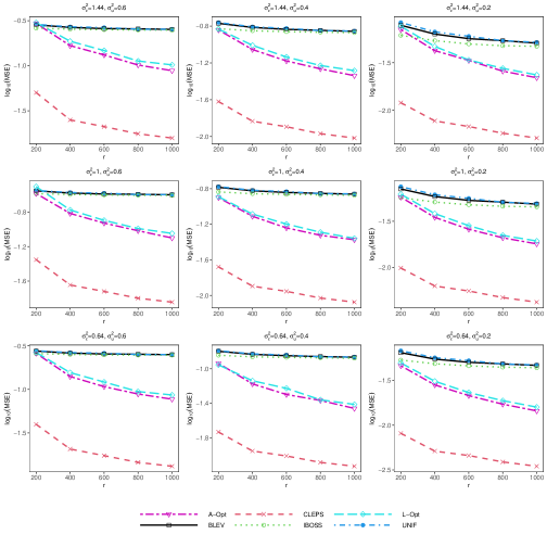
Figure 2: The MSEs based on different $\sigma_{u}^{2}$ and $\sigma_{\epsilon}^{2}$ for different $r$.

The results presented in Figure 2 demonstrate the superior performance of CLEPS compared to other methods, closely followed by the A-opt and L-opt. Furthermore, as the subsample size increases, the MSEs of our proposed methods approach to zero, while other approaches that do not account for measurement errors show relatively stable MSEs. These results confirm the inconsistency of ordinary least squares estimator for linear models with measurement errors. Additionally, decreasing $\sigma_{u}^{2}$ and $\sigma_{\epsilon}^{2}$ lead to a reductions for MSEs obtained by all six methods. Notably, even for big variance of the random error, our methods maintain good performance.

To further investigate the impact of other parameters on the sampling method, Figure 3 offers the variations in MSE across distinct values of $r_{0},n,p,$ and $m$ while keeping $\sigma_{\epsilon}^{2}=1$ and $\sigma_{u}^{2}=0.4$. Additionally, Table 1 presents the results about different $m$ for CLEPS.

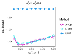
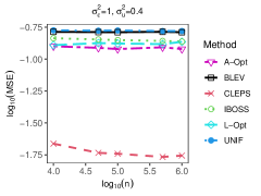
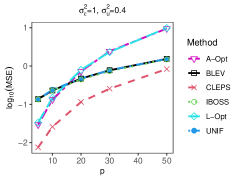
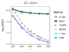
Figure 3: The plots except the bottom right present the MSEs for different $r_{0},n,p$, respectively. The bottom right plot presents the MSEs for different $r$ with $m=1$.

In Figure 3, the top left plot shows that as $r_{0}$ ascends, the performance of A-opt and L-opt initially enhances and subsequently declines for fixed $r_{0}+r=1000$. This reason is that the inaccurate estimation is obtained in the first step when $r_{0}$ is too small. The top right plot indicates that as the sample size increases, the CLEPS performs more efficiently, while other methods remain almost unchanged. The bottom left plot displays that as the dimension $p$ increases, the MSEs of various methods rises. When $p>15$, A-opt and L-opt underperform compared to other methods, whereas the CLEPS consistently demonstrates the best performance. The bottom right plot shows that when $m=1$, the MSE of CLEPS is slightly bigger than the A-opt and L-opt.

Table 1: The MSEs for different $m$.

	$m=1$	$m=10$	$m=20$	$m=30$	$m=50$
200	$-$0.775	$-$1.669	$-$1.880	$-$1.978	$-$2.085
400	$-$1.003	$-$1.864	$-$2.038	$-$2.128	$-$2.198
600	$-$1.156	$-$1.958	$-$2.111	$-$2.173	$-$2.244
800	$-$1.236	$-$2.034	$-$2.158	$-$2.212	$-$2.269
1000	$-$1.336	$-$2.075	$-$2.197	$-$2.244	$-$2.285

In Table 1, it is observed that as $m$ increases, the MSE decreases. However, the rate of reduction in MSE progressively diminishes. This suggests that $m$ should be significantly smaller than $r$ in order to achieve effective inference. It is advisable to set $m<r/10$, in accordance with the findings in Shang and Cheng (2017), Wang (2019b), and Wang and Ma (2021), which suggest that the number of partitions should be significantly smaller than the sample size within each data partition.

6 Real examples

6.1 Diamond price dataset

The diamond price dataset is an integrated dataset containing prices and other characteristics of approximately 54,000 diamonds. This dataset can be accessed at https://www.kaggle.com/datasets/shivam2503/diamonds. Our aim is to explore the relationship between diamond prices ($y$) and three covariates: carat ($x_{1}$), depth ($x_{2}$) and table ($x_{3}$). All variables are standardized and the linear model is

$$y=x_{1}\beta_{1}+x_{2}\beta_{2}+x_{3}\beta_{3}+\epsilon.$$

Following the literature, the measurement error model is $\mathbf{W}=\mathbf{X}+\mathbf{U}$, where $\mathbf{X}=(x_{1},x_{2},x_{3})^{T}$, $\mathbf{U}$ is the measurement error vector with mean zero and covariance matrix $\sigma_{u}^{2}I_{3}$, $\sigma_{u}^{2}=0.6,0.4,0.2$. Figure 4 depicts MSEs for different $\sigma_{u}^{2}$ and $r$ values when $m=10,r_{0}=200,N=500$. As the sample size increases, the MSEs of the proposed methods decrease and become smaller than those of other methods. Moreover, with an increase in the variance of measurement error, there is a corresponding decrease in the MSEs of the proposed methods.

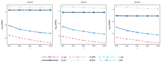
Figure 4: The MSEs for different $\sigma_{u}^{2}$ and $r$.

6.2 Airline delay dataset

The airline delay dataset has nearly 120 million records, which can be found in https://community.amstat.org/jointscsg-section/dataexpo/dataexpo2009. It includes detailed information on the arrival and departure of all commercial flights within the America from 1987 to 2008. This study focuses solely on 2008 data, yielding a total of 2389217 samples and 29 variables. After cleaning, 715731 observation data points were obtained. We select Arrival Delay as the response variable, with Departure Delay, Distance, Air Time, and Elapsed Time as the covariates. It’s worth noting that the flight elapsed time incorporates two types of time: Actual Elapsed Time and CRS Elapsed Time. Among them, the CRS Elapsed Time refers to the original elapsed time. Therefore, the Flight Elapsed Time is regarded as a variable with measurement errors of two repetitions, while other variables have no measurement errors. The estimate for the covariance matrix of measurement error is

$$\begin{bmatrix}0&&&\\ &0&&\\ &&0&\\ &&&0.0195\end{bmatrix}.$$

In our proposed methods, the Flight Elapsed Time is calculated as the mean of the two variables, whereas in other methods, it is determined as the Actual Elapsed Time.

Figure 5 displays the impact of varying $r$ on MSE when $m=10,r_{0}=200$, and $N=500$. Notably, the MSEs of the proposed methods consistently decrease and outperform other methods, indicating that our methods also have good properties in applications when $\boldsymbol{\Sigma}_{uu}$ is unknown.

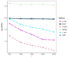
Figure 5: The MSEs for different $r$.

7 Summary

For large-scale data with measurement errors in covariates of linear models, this paper studies two subsampling methods based on the corrected likelihood. Theoretical results and numerical studies demonstrate that the two algorithms proposed in this paper outperform other existed sampling methods when measurement errors are present. However, this work only considers linear models. Future research directions could include investigating nonlinear models, high-dimensional data, or distributed data.

Supplementary Materials

Theorems 1-7 are proved in supplementary materials.

School of Statistics and Data Science, Qufu Normal University E-mail: 1819902359@qq.com

School of Statistics and Data Science, Qufu Normal University E-mail: mqwang@vip.126.com

School of Statistics and Data Science, Qufu Normal University E-mail: zhaoshli758@126.com

SUBSAMPLING FOR BIG DATA LINEAR MODELS

WITH MEASUREMENT ERRORS

School of Statistics and Data Science, Qufu Normal University

Supplementary Material

The supplementary material contains proofs for Theorems 1-7.

S1 Lemma

We first state a technical lemma.

Lemma 2 ($C_{r}$ inequality).

Let $\{X_{i},i\geq 1\}$ be a sequence of independent random variables, then the $k$-th moment of the sum of random variables is not greater than the sum of the $k$-th moments of the random variables. i.e.,

$$E\Big{|}\sum_{i=1}^{n}X_{i}\Big{|}^{k}\leq C_{r}\sum_{i=1}^{n}E|X_{i}|^{k},$$

where $C_{r}=\left\{\begin{aligned} &1,&&0<k\leq 1,\\ &n^{k-1},&&k>1.\end{aligned}\right.$

S2 Proof of Theorem 1

Note that

$$\tilde{\boldsymbol{\beta}}-\hat{\boldsymbol{\beta}} =(\frac{1}{n}\sum_{i=1}^{r}\frac{1}{r\pi_{i}^{*}}\mathbf{W}_{i}^{*}\mathbf{W}_{i}^{*T}-\boldsymbol{\Sigma}_{uu})^{-1}\cdot[\frac{1}{n}\sum_{i=1}^{r}\frac{1}{r\pi_{i}^{*}}\mathbf{W}_{i}^{*}(y_{i}^{*}-\mathbf{W}_{i}^{*T}\hat{\boldsymbol{\beta}})+\boldsymbol{\Sigma}_{uu}\hat{\boldsymbol{\beta}}]$$ (S2.1)

$$=-(\tilde{\mathcal{H}}_{W})^{-1}\dot{\ell}^{*}(\hat{\boldsymbol{\beta}}),$$

where $\tilde{\mathcal{H}}_{W}=\frac{1}{r}\sum_{i=1}^{r}[\frac{1}{n\pi_{i}^{*}}\mathbf{W}_{i}^{*}\mathbf{W}_{i}^{*T}-\boldsymbol{\Sigma}_{uu}],\dot{\ell}^{*}(\boldsymbol{\beta})=\frac{1}{n}\sum_{i=1}^{r}\frac{1}{r\pi_{i}^{*}}[-\mathbf{W}_{i}^{*}(y_{i}^{*}-\mathbf{W}_{i}^{*T}\boldsymbol{\beta})]-\boldsymbol{\Sigma}_{uu}\boldsymbol{\beta}.$ Therefore, we only need to prove

$$\dot{\ell}^{*}(\hat{\boldsymbol{\beta}})=O_{P|\mathcal{F}_{n}}(r^{-1/2}),$$ (S2.2)

and

$$\tilde{\mathcal{H}}_{W}-\mathcal{H}_{W}=O_{P|\mathcal{F}_{n}}(r^{-1/2}),$$ (S2.3)

where $\mathcal{H}_{W}=\frac{1}{n}\sum_{i=1}^{n}\mathbf{W}_{i}\mathbf{W}_{i}^{T}-\boldsymbol{\Sigma}_{uu}.$

To prove (S2.2), we directly calculate

$$E(\dot{\ell}^{*}(\hat{\boldsymbol{\beta}})|\mathcal{F}_{n}) =E\left\{\frac{1}{n}\sum_{i=1}^{r}\frac{1}{r\pi_{i}^{*}}[-\mathbf{W}_{i}^{*}(y_{i}^{*}-\mathbf{W}_{i}^{*T}\hat{\boldsymbol{\beta}})]-\boldsymbol{\Sigma}_{uu}\hat{\boldsymbol{\beta}}\bigg{|}\mathcal{F}_{n}\right\}$$

$$=\frac{1}{nr}\sum_{i=1}^{r}E\left\{\frac{1}{\pi_{i}^{*}}[-\mathbf{W}_{i}^{*}(y_{i}^{*}-\mathbf{W}_{i}^{*T}\hat{\boldsymbol{\beta}})]\Big{|}\mathcal{F}_{n}\right\}-\boldsymbol{\Sigma}_{uu}\hat{\boldsymbol{\beta}}$$

$$=\frac{1}{n}\sum_{i=1}^{n}\pi_{i}\cdot\frac{1}{\pi_{i}}[-\mathbf{W}_{i}(y_{i}-\mathbf{W}_{i}^{T}\hat{\boldsymbol{\beta}})]-\boldsymbol{\Sigma}_{uu}\hat{\boldsymbol{\beta}}$$

$$=\frac{1}{n}\sum_{i=1}^{n}[-\mathbf{W}_{i}(y_{i}-\mathbf{W}_{i}^{T}\hat{\boldsymbol{\beta}})]-\boldsymbol{\Sigma}_{uu}\hat{\boldsymbol{\beta}}$$

$$=\mathbf{0}.$$

For the $j$-th element $\dot{\ell}_{j}^{*}(\hat{\boldsymbol{\beta}})$ of $\dot{\ell}^{*}(\hat{\boldsymbol{\beta}})$ where $1\leq j\leq p$,

$$Var(\dot{\ell}_{j}^{*}(\hat{\boldsymbol{\beta}})|\mathcal{F}_{n})= E\left\{\frac{1}{n}\sum_{i=1}^{r}\frac{1}{r\pi_{i}^{*}}[-w_{ij}^{*}(y_{i}^{*}-\mathbf{W}_{i}^{*T}\hat{\boldsymbol{\beta}})]-(\boldsymbol{\Sigma}_{uu}\hat{\boldsymbol{\beta}})_{j}\bigg{|}\mathcal{F}_{n}\right\}^{2}$$

$$= E\left\{\frac{1}{r}\sum_{i=1}^{r}\left\{\frac{1}{n\pi_{i}^{*}}[-w_{ij}^{*}(y_{i}^{*}-\mathbf{W}_{i}^{*T}\hat{\boldsymbol{\beta}})]-(\boldsymbol{\Sigma}_{uu}\hat{\boldsymbol{\beta}})_{j}\right\}\bigg{|}\mathcal{F}_{n}\right\}^{2}$$

$$= \frac{1}{r^{2}}\sum_{i=1}^{r}E\left\{\frac{1}{n\pi_{i}^{*}}[-w_{ij}^{*}(y_{i}^{*}-\mathbf{W}_{i}^{*T}\hat{\boldsymbol{\beta}})]-(\boldsymbol{\Sigma}_{uu}\hat{\boldsymbol{\beta}})_{j}\Big{|}\mathcal{F}_{n}\right\}^{2}$$

$$= \frac{1}{r}\Bigg{\{}E\left\{\frac{1}{n\pi_{i}^{*}}[-w_{ij}^{*}(y_{i}^{*}-\mathbf{W}_{i}^{*T}\hat{\boldsymbol{\beta}})]\Big{|}\mathcal{F}_{n}\right\}^{2}+E[(\boldsymbol{\Sigma}_{uu}\hat{\boldsymbol{\beta}})_{j}|\mathcal{F}_{n}]^{2}$$

$$-2E\left[\frac{1}{n\pi_{i}^{*}}[-w_{ij}^{*}(y_{i}^{*}-\mathbf{W}_{i}^{*T}\hat{\boldsymbol{\beta}})](\boldsymbol{\Sigma}_{uu}\hat{\boldsymbol{\beta}})_{j}\Big{|}\mathcal{F}_{n}\right]\Bigg{\}}$$

$$= \frac{1}{n^{2}r}\sum_{i=1}^{n}\pi_{i}\cdot\left\{\frac{1}{\pi_{i}}[-w_{ij}(y_{i}-\mathbf{W}_{i}^{T}\hat{\boldsymbol{\beta}})]\right\}^{2}-\frac{1}{r}(\boldsymbol{\Sigma}_{uu}\hat{\boldsymbol{\beta}})_{j}^{2}$$

$$= \frac{1}{n^{2}r}\sum_{i=1}^{n}\frac{w_{ij}^{2}(y_{i}-\mathbf{W}_{i}^{T}\hat{\boldsymbol{\beta}})^{2}}{\pi_{i}}-\frac{1}{r}(\boldsymbol{\Sigma}_{uu}\hat{\boldsymbol{\beta}})_{j}^{2}$$

$$\leq \frac{1}{r}\max_{i=1,\ldots,n}(n\pi_{i})^{-1}\sum_{i=1}^{n}\frac{\|\mathbf{W}_{i}\|^{2}(y_{i}-\mathbf{W}_{i}^{T}\hat{\boldsymbol{\beta}})^{2}}{n}-\frac{1}{r}(\boldsymbol{\Sigma}_{uu}\hat{\boldsymbol{\beta}})_{j}^{2}.$$

By Assumption 2 and Holder inequality, we can achieve

$$\sum_{i=1}^{n}\frac{\|\mathbf{W}_{i}\|^{2}(y_{i}-\mathbf{W}_{i}^{T}\hat{\boldsymbol{\beta}})^{2}}{n}\leq\left(\sum_{i=1}^{n}\frac{\|\mathbf{W}_{i}\|^{4}}{n}\right)^{1/2}\left(\sum_{i=1}^{n}\frac{(y_{i}-\mathbf{W}_{i}^{T}\hat{\boldsymbol{\beta}})^{4}}{n}\right)^{1/2}=O_{P}(1).$$ (S2.4)

According to Assumption 3, we can infer that $Var(\dot{\ell}_{j}^{*}(\hat{\boldsymbol{\beta}})|\mathcal{F}_{n})=\frac{1}{r}O_{P}(1)O_{P}(1)-O_{P}(r^{-1})=O_{P}(r^{-1})$. From the Chebyshev inequality, for a sufficiently large $M$, we have

$$P(\|\dot{\ell}^{*}(\hat{\boldsymbol{\beta}})\|\geq r^{-1/2}M|\mathcal{F}_{n}) \leq\frac{rE(\|\dot{\ell}^{*}(\hat{\boldsymbol{\beta}})\|^{2}|\mathcal{F}_{n})}{M^{2}}$$

$$=\frac{r\sum_{j=1}^{p}E(\dot{\ell}_{j}^{*}(\hat{\boldsymbol{\beta}})^{2}|\mathcal{F}_{n})}{M^{2}}$$

$$=\frac{O_{P}(1)}{M^{2}}\rightarrow 0,n,r\rightarrow\infty.$$

Thus, the equation (S2.2) is derived.

In order to prove (S2.3), we directly calculate

$$E(\tilde{\mathcal{H}}_{W}|\mathcal{F}_{n})=\mathcal{H}_{W}.$$

For any element $\tilde{\mathcal{H}}_{W}^{j_{1}j_{2}},1\leq j_{1},j_{2}\leq p$ of $\tilde{\mathcal{H}}_{W}$, using Assumptions 2, 3 and Cauchy-Schwarz inequality, it can be concluded that

$$Var(\tilde{\mathcal{H}}_{W}^{j_{1}j_{2}}|\mathcal{F}_{n})= E\{\tilde{\mathcal{H}}_{W}^{j_{1}j_{2}}-\mathcal{H}_{W}^{j_{1}j_{2}}|\mathcal{F}_{n}\}^{2}$$

$$= E\left\{\frac{1}{nr}\sum_{i=1}^{r}\frac{1}{\pi_{i}^{*}}w_{ij_{1}}^{*}w_{ij_{2}}^{*}-\frac{1}{n}\sum_{i=1}^{n}w_{ij_{1}}w_{ij_{2}}\bigg{|}\mathcal{F}_{n}\right\}^{2}$$

$$= E\left(\frac{1}{nr}\sum_{i=1}^{r}\frac{1}{\pi_{i}^{*}}w_{ij_{1}}^{*}w_{ij_{2}}^{*}|\mathcal{F}_{n}\right)^{2}-\left(\frac{1}{n}\sum_{i=1}^{n}w_{ij_{1}}w_{ij_{2}}\right)^{2}$$

$$= \frac{1}{n^{2}r}\sum_{i=1}^{n}\pi_{i}\cdot\left(\frac{w_{ij_{1}}w_{ij_{2}}}{\pi_{i}}\right)^{2}-\frac{1}{n^{2}}\sum_{i=1}^{n}(w_{ij_{1}}w_{ij_{2}})^{2}$$

$$= \frac{1}{n^{2}r}\sum_{i=1}^{n}\frac{(w_{ij_{1}}w_{ij_{2}})^{2}}{\pi_{i}}-\frac{1}{n^{2}}\sum_{i=1}^{n}(w_{ij_{1}}w_{ij_{2}})^{2}$$

$$\leq \frac{1}{r}\max_{i=1,\ldots,n}(n\pi_{i})^{-1}\sum_{i=1}^{n}\frac{\|\mathbf{W}_{i}\|^{4}}{n}$$

$$= \frac{1}{r}O_{P}(1)O_{P}(1)=O_{P}(r^{-1}).$$

Using the Chebyshev inequality, for sufficiently large $M$, we have

$$P(\|\tilde{\mathcal{H}}_{W}-\mathcal{H}_{W}\|\geq r^{-1/2}M|\mathcal{F}_{n}) \leq\frac{rE(\|\tilde{\mathcal{H}}_{W}\|^{2}|\mathcal{F}_{n})}{M^{2}}$$

$$=\frac{r\sum_{j_{1}=1}^{p}\sum_{j_{2}=1}^{p}E(\tilde{\mathcal{H}}_{W}^{j_{1}j_{2}}|\mathcal{F}_{n})^{2}}{M^{2}}$$

$$=\frac{O_{P}(1)}{M^{2}}\rightarrow 0,n,r\rightarrow\infty.$$

Thus, the equation (S2.3) is proved.

By (S2.3) and Assumption 1, we can obtain $\tilde{\mathcal{H}}_{W}^{-1}=O_{P|\mathcal{F}_{n}}(1)$. Therefore, combining (S2.1), (S2.2) and (S2.3), we have

$$\tilde{\boldsymbol{\beta}}-\hat{\boldsymbol{\beta}}=O_{P|\mathcal{F}_{n}}(r^{-1/2}).$$

Then the theorem is proved.

S3 Proof of Theorem 2

Note that

$$\dot{\ell}^{*}(\hat{\boldsymbol{\beta}})=\frac{1}{r}\sum_{i=1}^{r}\left\{\frac{1}{n\pi_{i}^{*}}[-\mathbf{W}_{i}^{*}(y_{i}^{*}-\mathbf{W}_{i}^{*T}\hat{\boldsymbol{\beta}})]-\boldsymbol{\Sigma}_{uu}\hat{\boldsymbol{\beta}}\right\}=\frac{1}{r}\sum_{i=1}^{r}\boldsymbol{\xi}_{i},$$ (S3.1)

where $\boldsymbol{\xi}_{i}=\frac{1}{n\pi_{i}^{*}}[-\mathbf{W}_{i}^{*}(y_{i}^{*}-\mathbf{W}_{i}^{*T}\hat{\boldsymbol{\beta}})]-\boldsymbol{\Sigma}_{uu}\hat{\boldsymbol{\beta}}$ is an independent random vector. Then it can be directly calculated to obtain

$$E(\boldsymbol{\xi}_{i}|\mathcal{F}_{n}) =\frac{1}{n}\sum_{i=1}^{n}[-\mathbf{W}_{i}(y_{i}-\mathbf{W}_{i}^{T}\hat{\boldsymbol{\beta}})]-\boldsymbol{\Sigma}_{uu}\hat{\boldsymbol{\beta}}=\mathbf{0},$$ (S3.2)

$$Var(\boldsymbol{\xi}_{i}|\mathcal{F}_{n}) =\frac{1}{n^{2}}\sum_{i=1}^{n}\frac{\mathbf{W}_{i}\mathbf{W}_{i}^{T}(y_{i}-\mathbf{W}_{i}^{T}\hat{\boldsymbol{\beta}})^{2}}{\pi_{i}}-(\boldsymbol{\Sigma}_{uu}\hat{\boldsymbol{\beta}})^{\otimes 2}=rV_{c}.$$

According to the $C_{r}$ inequality, Assumptions 3 and 4, we have

$$\sum_{i=1}^{r}E\{\|r^{-1/2}\boldsymbol{\xi}_{i}\|^{2}I(\|r^{-1/2}\boldsymbol{\xi}_{i}\|>\varepsilon)|\mathcal{F}_{n}\}$$

$$\leq \frac{1}{\varepsilon^{\delta}r^{1+\delta/2}}\sum_{i=1}^{r}E\{\|\boldsymbol{\xi}_{i}\|^{2+\delta}|\mathcal{F}_{n}\}$$

$$= \frac{1}{\varepsilon^{\delta}r^{1+\delta/2}}\sum_{i=1}^{r}E\left\{\left\|\frac{1}{n\pi_{i}^{*}}[-\mathbf{W}_{i}^{*}(y_{i}^{*}-\mathbf{W}_{i}^{*T}\hat{\boldsymbol{\beta}})]-\boldsymbol{\Sigma}_{uu}\hat{\boldsymbol{\beta}}\right\|^{2+\delta}\bigg{|}\mathcal{F}_{n}\right\}$$

$$\leq \frac{2^{1+\delta}}{\varepsilon^{\delta}r^{1+\delta/2}}\sum_{i=1}^{r}\left\{E\left[\left\|\frac{1}{n\pi_{i}^{*}}\mathbf{W}_{i}^{*}(y_{i}^{*}-\mathbf{W}_{i}^{*T}\hat{\boldsymbol{\beta}})\right\|^{2+\delta}|\mathcal{F}_{n}\right]+E[\|\boldsymbol{\Sigma}_{uu}\hat{\boldsymbol{\beta}}\|^{2+\delta}|\mathcal{F}_{n}]\right\}$$

$$= \frac{2^{1+\delta}}{\varepsilon^{\delta}r^{\delta/2}}\left\{\sum_{i=1}^{n}\frac{\|\mathbf{W}_{i}\|^{2+\delta}(y_{i}-\mathbf{W}_{i}^{T}\hat{\boldsymbol{\beta}})^{2+\delta}}{n^{2+\delta}\pi_{i}^{1+\delta}}+\|\boldsymbol{\Sigma}_{uu}\hat{\boldsymbol{\beta}}\|^{2+\delta}\right\}$$

$$\leq \frac{2^{1+\delta}}{\varepsilon^{\delta}r^{\delta/2}}\left\{\max_{i=1,\ldots,n}(n\pi_{i})^{-1-\delta}\sum_{i=1}^{n}\frac{(y_{i}-\mathbf{W}_{i}^{T}\hat{\boldsymbol{\beta}})^{2+\delta}\|\mathbf{W}_{i}\|^{2+\delta}}{n}+\|\boldsymbol{\Sigma}_{uu}\hat{\boldsymbol{\beta}}\|^{2+\delta}\right\}$$

$$= O_{P}(r^{-\delta/2}).$$

In the light of the Lindeberg-Feller central limit theorem, it follows that

$$\left(\sum_{i=1}^{r}Var(\boldsymbol{\xi}_{i}|\mathcal{F}_{n})\right)^{-1/2}\sum_{i=1}^{r}\boldsymbol{\xi}_{i}=V_{c}^{-1/2}\dot{\ell}^{*}(\hat{\boldsymbol{\beta}})\xrightarrow{d}N_{p}(\mathbf{0},I).$$ (S3.3)

By (S2.3), we can obtain

$$\tilde{\mathcal{H}}_{W}^{-1}-\mathcal{H}_{W}^{-1}=-\mathcal{H}_{W}^{-1}(\tilde{\mathcal{H}}_{W}-\mathcal{H}_{W})\tilde{\mathcal{H}}_{W}^{-1}=O_{P|\mathcal{F}_{n}}(r^{-1/2}).$$ (S3.4)

By Assumption 1, $\mathcal{H}_{W}$ converges to a positive definite matrix, then $\mathcal{H}_{W}^{-1}=O_{P}(1)$. And due to (S3.2), we have

$$V=\mathcal{H}_{W}^{-1}V_{c}\mathcal{H}_{W}^{-1}=\frac{1}{r}\mathcal{H}_{W}^{-1}(rV_{c})\mathcal{H}_{W}^{-1}=O_{P}(r^{-1}).$$ (S3.5)

Therefore, combining (S2.1), (S3.4) and (S3.5), then

$$V^{-1/2}(\tilde{\boldsymbol{\beta}}-\hat{\boldsymbol{\beta}}) =-V^{-1/2}\tilde{\mathcal{H}}_{W}^{-1}\dot{\ell}^{*}(\hat{\boldsymbol{\beta}})$$

$$=-V^{-1/2}\mathcal{H}_{W}^{-1}\dot{\ell}^{*}(\hat{\boldsymbol{\beta}})-V^{-1/2}(\tilde{\mathcal{H}}_{W}^{-1}-\mathcal{H}_{W}^{-1})\dot{\ell}^{*}(\hat{\boldsymbol{\beta}})$$

$$=-V^{-1/2}\mathcal{H}_{W}^{-1}V_{c}^{1/2}V_{c}^{-1/2}\dot{\ell}^{*}(\hat{\boldsymbol{\beta}})+O_{P|\mathcal{F}_{n}}(r^{-1/2}).$$

Note that

$$V^{-1/2}\mathcal{H}_{W}^{-1}V_{c}^{1/2}(V^{-1/2}\mathcal{H}_{W}^{-1}V_{c}^{1/2})^{T}=V^{-1/2}\mathcal{H}_{W}^{-1}V_{c}^{1/2}V_{c}^{1/2}\mathcal{H}_{W}^{-1}V^{-1/2}=I,$$

According to the Slutsky theorem, we have

$$V^{-1/2}(\tilde{\boldsymbol{\beta}}-\hat{\boldsymbol{\beta}})\xrightarrow{d}N_{p}(\mathbf{0},I),r,n\rightarrow\infty.$$ (S3.6)

Then the theorem is proved.

S4 Proof of Theorem 3

First of all, we prove(i). Let $V_{c}^{*}=\frac{1}{rn^{2}}\sum_{i=1}^{n}\frac{(y_{i}-\mathbf{W}_{i}^{T}\hat{\boldsymbol{\beta}})^{2}\mathbf{W}_{i}\mathbf{W}_{i}^{T}}{\pi_{i}}$. Note that $V_{c}=V_{c}^{*}-\frac{1}{r}(\boldsymbol{\Sigma}_{uu}\boldsymbol{\beta})^{\otimes 2}$, the second item is not related to $\pi_{i}$. Therefore, to minimize $tr(V)$, we need to minimize $tr(\mathcal{H}_{W}^{-1}V_{c}^{*}\mathcal{H}_{W}^{-1})$. Then, we have

$$tr(\mathcal{H}_{W}^{-1}V_{c}^{*}\mathcal{H}_{W}^{-1}) =\frac{1}{rn^{2}}\sum_{i=1}^{n}tr\left[\frac{(y_{i}-\mathbf{W}_{i}^{T}\hat{\boldsymbol{\beta}})^{2}\mathcal{H}_{W}^{-1}\mathbf{W}_{i}\mathbf{W}_{i}^{T}\mathcal{H}_{W}^{-1}}{\pi_{i}}\right]$$

$$=\frac{1}{rn^{2}}\sum_{i=1}^{n}\frac{(y_{i}-\mathbf{W}_{i}^{T}\hat{\boldsymbol{\beta}})^{2}\mathcal{\|}\mathcal{H}_{W}^{-1}\mathbf{W}_{i}\|^{2}}{\pi_{i}}$$

$$=\frac{1}{rn^{2}}\sum_{i=1}^{n}\pi_{i}\sum_{i=1}^{n}\frac{(y_{i}-\mathbf{W}_{i}^{T}\hat{\boldsymbol{\beta}})^{2}\|\mathcal{H}_{W}^{-1}\mathbf{W}_{i}\|^{2}}{\pi_{i}}$$

$$\geq\frac{1}{rn^{2}}\left[\sum_{i=1}^{n}|y_{i}-\mathbf{W}_{i}^{T}\hat{\boldsymbol{\beta}}|\cdot\|\mathcal{H}_{W}^{-1}\mathbf{W}_{i}\|\right]^{2}.$$

The last inequality sign is the application of the Cauchy-Schwarz inequality. The equation holds only if and when $\pi_{i}\propto|y_{i}-\mathbf{W}_{i}^{T}\hat{\boldsymbol{\beta}}|\cdot\|\mathcal{H}_{W}^{-1}\mathbf{W}_{i}\|$. (ii) can be proved in the same way, so we omit the proof details here.

S5 Proof of Theorems 4 and 5

Since the proof methods of these two theorems are similar to those of Theorems 1 and 2, and Wang, Zhu and Ma(2018) have provided specific proof methods, we omit the proofs of these two theorems here.

S6 Proof of Theorem 6

First, we consider the case where $m=1$. Note that

$$\check{\boldsymbol{\beta}}-\hat{\boldsymbol{\beta}} =\left(\frac{1}{n}\sum_{i=1}^{n}\psi_{i}\mathbf{W}_{i}\mathbf{W}_{i}^{T}-\boldsymbol{\Sigma}_{uu}\right)^{-1}\cdot\left[\frac{1}{n}\sum_{i=1}^{n}\psi_{i}\mathbf{W}_{i}(y_{i}-\mathbf{W}_{i}^{T}\hat{\boldsymbol{\beta}})+\boldsymbol{\Sigma}_{uu}\hat{\boldsymbol{\beta}}\right]$$ (S6.1)

$$=-(\check{\mathcal{H}}_{W})^{-1}\dot{L}^{*}(\hat{\boldsymbol{\beta}}),$$

where $\check{\mathcal{H}}_{W}=\frac{1}{n}\sum_{i=1}^{n}\psi_{i}(\mathbf{W}_{i}\mathbf{W}_{i}^{T})-\boldsymbol{\Sigma}_{uu},\dot{L}^{*}(\boldsymbol{\beta})=\frac{1}{n}\sum_{i=1}^{n}\psi_{i}[-\mathbf{W}_{i}(y_{i}-\mathbf{W}_{i}^{T}\boldsymbol{\beta})]\\ -\boldsymbol{\Sigma}_{uu}\boldsymbol{\beta}.$ Therefore, it is only necessary to demonstrate that

$$\dot{L}^{*}(\hat{\boldsymbol{\beta}})=O_{P|\mathcal{F}_{n}}(r^{-1/2}),$$ (S6.2)

and

$$\check{\mathcal{H}}_{W}-\mathcal{H}_{W}=O_{P|\mathcal{F}_{n}}(r^{-1/2}),$$ (S6.3)

where $\mathcal{H}_{W}=\frac{1}{n}\sum_{i=1}^{n}\mathbf{W}_{i}\mathbf{W}_{i}^{T}-\boldsymbol{\Sigma}_{uu}.$

Note that

$$E(\psi_{i})=E(\mu_{i}\nu_{i})=q_{n}\cdot\frac{1}{q_{n}}=1,$$

$$E(\psi_{i}^{2})=(q_{n}(1-q_{n})+q_{n}^{2})\cdot\left(b_{n}^{2}+\frac{1}{q_{n}^{2}}\right)=q_{n}b_{n}^{2}+\frac{1}{q_{n}},$$

and

$$Var(\psi_{i})=E(\psi_{i}^{2})-(E(\psi_{i}))^{2}=q_{n}b_{n}^{2}+\frac{1}{q_{n}}-1=\frac{na_{n}}{r},$$

where $a_{n}=b_{n}^{2}q_{n}^{2}-q_{n}+1.$ According to the Assumption 5, as $q_{n}\rightarrow 0$, $\limsup\limits_{n\rightarrow\infty}a_{n}=\limsup\limits_{n\rightarrow\infty}q_{n}Var(\psi)=\limsup\limits_{n\rightarrow\infty}q_{n}(E(\psi_{i}^{2})-1)=<\infty.$

To prove (S6.2), we calculate directly to obtain

$$E(\dot{L}^{*}(\hat{\boldsymbol{\beta}})|\mathcal{F}_{n}) =E\left\{\frac{1}{n}\sum_{i=1}^{n}\psi_{i}[-\mathbf{W}_{i}(y_{i}-\mathbf{W}_{i}^{T}\hat{\boldsymbol{\beta}})]-\boldsymbol{\Sigma}_{uu}\hat{\boldsymbol{\beta}}\bigg{|}\mathcal{F}_{n}\right\}$$

$$=\frac{1}{n}\sum_{i=1}^{n}[-\mathbf{W}_{i}(y_{i}-\mathbf{W}_{i}^{T}\hat{\boldsymbol{\beta}})]-\boldsymbol{\Sigma}_{uu}\hat{\boldsymbol{\beta}}=\mathbf{0}.$$

For the $j$-th element of $\dot{L}^{*}(\hat{\boldsymbol{\beta}})$, represented as $\dot{L}_{j}^{*}(\hat{\boldsymbol{\beta}})=\frac{1}{n}\sum_{i=1}^{n}\psi_{i}[-w_{ij}(y_{i}-\mathbf{W}_{i}^{T}\hat{\boldsymbol{\beta}})]-(\boldsymbol{\Sigma}_{uu}\hat{\boldsymbol{\beta}})_{j}$. By (S2.4) and Assumption 6, we have

$$Var(\dot{L}_{j}^{*}(\hat{\boldsymbol{\beta}})|\mathcal{F}_{n}) =Var\left\{\frac{1}{n}\sum_{i=1}^{n}\psi_{i}[-w_{ij}(y_{i}-\mathbf{W}_{i}^{T}\hat{\boldsymbol{\beta}})]-(\boldsymbol{\Sigma}_{uu}\hat{\boldsymbol{\beta}})_{j}\bigg{|}\mathcal{F}_{n}\right\}$$

$$=\frac{1}{n^{2}}\frac{na_{n}}{r}\sum_{i=1}^{n}w_{ij}^{2}(y_{i}-\mathbf{W}_{i}^{T}\hat{\boldsymbol{\beta}})^{2}$$

$$\leq\frac{a_{n}}{r}\sum_{i=1}^{n}\frac{\|\mathbf{W}_{i}\|^{2}(y_{i}-\mathbf{W}_{i}^{T}\hat{\boldsymbol{\beta}})^{2}}{n}$$

$$=\frac{1}{r}O_{P}(1)=O_{P}(r^{-1}).$$

From the Chebyshev inequality, for sufficiently large $M$, we have

$$P(\|\dot{L}^{*}(\hat{\boldsymbol{\beta}})\|\geq r^{-1/2}M|\mathcal{F}_{n}) \leq\frac{rE(\|\dot{L}^{*}(\hat{\boldsymbol{\beta}})\|^{2}|\mathcal{F}_{n})}{M^{2}}$$

$$=\frac{r\sum_{j=1}^{p}E(\dot{L}_{j}^{*}(\hat{\boldsymbol{\beta}})|\mathcal{F}_{n})^{2}}{M^{2}}$$

$$=\frac{O_{P}(1)}{M^{2}}\rightarrow 0,n,r\rightarrow\infty.$$

Thus, the equation (S6.2) is proved.

To prove (S6.3), We calculate directly to obtain

$$E(\check{\mathcal{H}}_{W}|\mathcal{F}_{n})=\mathcal{H}_{W},$$

For any element $\check{\mathcal{H}}_{W}^{j_{1}j_{2}},1\leq j_{1},j_{2}\leq p$ of $\check{\mathcal{H}}_{W}$, by Assumptions 2 and 5, we have

$$Var(\check{\mathcal{H}}_{W}^{j_{1}j_{2}}|\mathcal{F}_{n}) =Var\left[\frac{1}{n}\sum_{i=1}^{n}\psi_{i}(W_{ij_{1}}W_{ij_{2}})-(\boldsymbol{\Sigma}_{uu})_{j_{1}j_{2}}\Big{|}\mathcal{F}_{n}\right]$$

$$=\frac{1}{n^{2}}\frac{na_{n}}{r}\sum_{i=1}^{n}(W_{ij_{1}}W_{ij_{2}})^{2}$$

$$\leq\frac{a_{n}}{r}\sum_{i=1}^{n}\frac{\|\mathbf{W}_{i}\|^{4}}{n}=\frac{1}{r}O_{P}(1)$$

$$=O_{P}(r^{-1}).$$

From the Chebyshev inequality, for sufficiently large $M$, we have

$$P(\|\check{\mathcal{H}}_{W}-\mathcal{H}_{W}\|\geq r^{-1/2}M|\mathcal{F}_{n}) \leq\frac{rE(\|\check{\mathcal{H}}_{W}\|^{2}|\mathcal{F}_{n})}{M^{2}}$$

$$=\frac{r\sum_{j_{1}=1}^{p}\sum_{j_{2}=1}^{p}E(\check{\mathcal{H}}_{W}^{j_{1}j_{2}}|\mathcal{F}_{n})^{2}}{M^{2}}$$

$$=\frac{O_{P}(1)}{M^{2}}\rightarrow 0,n,r\rightarrow\infty.$$

Thus, the equation (S6.3) is proved.

By (S6.3) and Assumption 1, we have $\check{\mathcal{H}}_{W}^{-1}=O_{P|\mathcal{F}_{n}}(1)$. Therefore, combining (S6.1), (S6.2) and (S6.3), then

$$\check{\boldsymbol{\beta}}-\hat{\boldsymbol{\beta}}=O_{P|\mathcal{F}_{n}}(r^{-1/2}).$$ (S6.4)

As $m>1$ , we have $\check{\boldsymbol{\beta}}^{(m)}=\frac{1}{m}\sum_{k=1}^{m}\check{\boldsymbol{\beta}}_{k}.$ Then according to the weak law of large numbers, it follows that

$$\check{\boldsymbol{\beta}}^{(m)}-\hat{\boldsymbol{\beta}}=\frac{1}{m}\sum_{k=1}^{m}\check{\boldsymbol{\beta}}_{k}-\hat{\boldsymbol{\beta}}=\frac{1}{m}\sum_{k=1}^{m}(\check{\boldsymbol{\beta}}_{k}-\hat{\boldsymbol{\beta}})=O_{P|\mathcal{F}_{n}}((mr)^{-1/2}).$$

Then the theorem is proved.

S7 Proof of Theorem 7

Firstly, we prove the case where $m=1$. Because

$$\dot{L}^{*}(\hat{\boldsymbol{\beta}})=\frac{1}{n}\sum_{i=1}^{n}\{\psi_{i}[-\mathbf{W}_{i}(y_{i}-\mathbf{W}_{i}^{T}\hat{\boldsymbol{\beta}})]-\boldsymbol{\Sigma}_{uu}\hat{\boldsymbol{\beta}}\}=\frac{1}{\sqrt{r}}\sum_{i=1}^{n}\boldsymbol{\eta}_{i},$$ (S7.1)

where $\boldsymbol{\eta}_{i}=\frac{\sqrt{r}}{n}\{\psi_{i}[-\mathbf{W}_{i}(y_{i}-\mathbf{W}_{i}^{T}\hat{\boldsymbol{\beta}})]-\boldsymbol{\Sigma}_{uu}\hat{\boldsymbol{\beta}}\}$ is an independent random vector. Note that

$$E(\boldsymbol{\eta}_{i}|\mathcal{F}_{n}) =\frac{\sqrt{r}}{n}[-\mathbf{W}_{i}(y_{i}-\mathbf{W}_{i}^{T}\hat{\boldsymbol{\beta}})-\boldsymbol{\Sigma}_{uu}\hat{\boldsymbol{\beta}}],$$

$$Var(\boldsymbol{\eta}_{i}|\mathcal{F}_{n}) =\frac{r}{n^{2}}\frac{na_{n}}{r}[-\mathbf{W}_{i}(y_{i}-\mathbf{W}_{i}^{T}\hat{\boldsymbol{\beta}})]^{\otimes 2}=\frac{a_{n}}{n}\mathbf{W}_{i}\mathbf{W}_{i}^{T}(y_{i}-\mathbf{W}_{i}^{T}\hat{\boldsymbol{\beta}})^{2}.$$

Then by using Assumptions 2 and 5, we obtain

$$\sum_{i=1}^{n}E(\boldsymbol{\eta}_{i}|\mathcal{F}_{n})=\frac{\sqrt{r}}{n}\sum_{i=1}^{n}[-\mathbf{W}_{i}(y_{i}-\mathbf{W}_{i}^{T}\hat{\boldsymbol{\beta}})-\boldsymbol{\Sigma}_{uu}\hat{\boldsymbol{\beta}}]=\mathbf{0},$$

$$\sum_{i=1}^{n}Var(\boldsymbol{\eta}_{i}|\mathcal{F}_{n})=\frac{a_{n}}{n}\sum_{i=1}^{n}\mathbf{W}_{i}\mathbf{W}_{i}^{T}(y_{i}-\mathbf{W}_{i}^{T}\hat{\boldsymbol{\beta}})^{2}=a_{n}\Sigma_{c}.$$ (S7.2)

According to the $C_{r}$ inequality, Assumptions 4 and 5, we have

$$\sum_{i=1}^{n}E\{\|\boldsymbol{\eta}_{i}\|^{2}I(\|\boldsymbol{\eta}_{i}\|>\varepsilon)|\mathcal{F}_{n}\}$$

$$\leq \varepsilon^{-\alpha}\sum_{i=1}^{n}E\{\|\boldsymbol{\eta}_{i}\|^{2+\alpha}|\mathcal{F}_{n}\}$$

$$= \varepsilon^{-\alpha}\sum_{i=1}^{n}E\left\{\left\|\frac{\sqrt{r}}{n}\{\psi_{i}[-\mathbf{W}_{i}(y_{i}-\mathbf{W}_{i}^{T}\hat{\boldsymbol{\beta}})]-\boldsymbol{\Sigma}_{uu}\hat{\boldsymbol{\beta}}\}\right\|^{2+\alpha}\bigg{|}\mathcal{F}_{n}\right\}$$

$$= \frac{r^{1+\frac{\alpha}{2}}}{\varepsilon^{\alpha}n^{2+\alpha}}\sum_{i=1}^{n}E\{\|\psi_{i}\mathbf{W}_{i}(y_{i}-\mathbf{W}_{i}^{T}\hat{\boldsymbol{\beta}})+\boldsymbol{\Sigma}_{uu}\hat{\boldsymbol{\beta}}\|^{2+\alpha}|\mathcal{F}_{n}\}$$

$$\leq \frac{r^{1+\frac{\alpha}{2}}2^{1+\alpha}}{\varepsilon^{\alpha}n^{2+\alpha}}\sum_{i=1}^{n}\{E[\|\psi_{i}\mathbf{W}_{i}(y_{i}-\mathbf{W}_{i}^{T}\hat{\boldsymbol{\beta}})\|^{2+\alpha}|\mathcal{F}_{n}]+E[\|\boldsymbol{\Sigma}_{uu}\hat{\boldsymbol{\beta}}\|^{2+\alpha}|\mathcal{F}_{n}]\}$$

$$= \frac{r^{1+\frac{\alpha}{2}}2^{1+\alpha}}{\varepsilon^{\alpha}n^{1+\alpha}}\left\{E(\psi)^{2+\alpha}\frac{1}{n}\sum_{i=1}^{n}\|\mathbf{W}_{i}\|^{2+\alpha}(y_{i}-\mathbf{W}_{i}^{T}\hat{\boldsymbol{\beta}})^{2+\alpha}+\|\boldsymbol{\Sigma}_{uu}\hat{\boldsymbol{\beta}}\|^{2+\alpha}\right\}$$

$$= O_{P}(r^{-\alpha/2}).$$

Therefore, the Lindeberg-Feller condition is satisfied. According to the Lindeberg-Feller central limit theorem, we have

$$\left(\sum_{i=1}^{n}Var(\boldsymbol{\eta}_{i}|\mathcal{F}_{n})\right)^{-1/2}\sum_{i=1}^{n}\boldsymbol{\eta}_{i}=\sqrt{\frac{r}{a_{n}}}\Sigma_{c}^{-1/2}\dot{L}^{*}(\hat{\boldsymbol{\beta}})\xrightarrow{d}N_{p}(\mathbf{0},I).$$ (S7.3)

By (S6.3), we have

$$\check{\mathcal{H}}_{W}^{-1}-\mathcal{H}_{W}^{-1}=-\mathcal{H}_{W}^{-1}(\check{\mathcal{H}}_{W}-\mathcal{H}_{W})\check{\mathcal{H}}_{W}^{-1}=O_{P|\mathcal{F}_{n}}(r^{-1/2}),$$ (S7.4)

By Assumption 1, $\mathcal{H}_{W}$ converges to a positive definite matrix, then $\mathcal{H}_{W}^{-1}=O_{P}(1)$. And due to (S7.2), we obtain

$$\Sigma=\mathcal{H}_{W}^{-1}\Sigma_{c}\mathcal{H}_{W}^{-1}=O_{P}(1).$$ (S7.5)

Therefore, combining(S6.1), (S7.4) and (S7.5), we have

$$\sqrt{\frac{r}{a_{n}}}\Sigma^{-1/2}(\check{\boldsymbol{\beta}}-\hat{\boldsymbol{\beta}}) =-\sqrt{\frac{r}{a_{n}}}\Sigma^{-1/2}\check{\mathcal{H}}_{W}^{-1}\dot{L}^{*}(\hat{\boldsymbol{\beta}})$$

$$=-\sqrt{\frac{r}{a_{n}}}\Sigma^{-1/2}\mathcal{H}_{W}^{-1}\dot{L}^{*}(\hat{\boldsymbol{\beta}})-\sqrt{\frac{r}{a_{n}}}\Sigma^{-1/2}(\check{\mathcal{H}}_{W}^{-1}-\mathcal{H}_{W}^{-1})\dot{L}^{*}(\hat{\boldsymbol{\beta}})$$

$$=-\sqrt{\frac{r}{a_{n}}}{\Sigma}^{-1/2}\mathcal{H}_{W}^{-1}\Sigma_{c}^{1/2}\Sigma_{c}^{-1/2}\dot{L}^{*}(\hat{\boldsymbol{\beta}})+O_{P|\mathcal{F}_{n}}(r^{-1/2}).$$

Note that

$$\Sigma^{-1/2}\mathcal{H}_{W}^{-1}\Sigma_{c}^{1/2}(\Sigma^{-1/2}\mathcal{H}_{W}^{-1}\Sigma_{c}^{1/2})^{T}=\Sigma^{-1/2}\mathcal{H}_{W}^{-1}\Sigma_{c}^{1/2}\Sigma_{c}^{1/2}\mathcal{H}_{W}^{-1}\Sigma^{-1/2}=I,$$

Using of the Slutsky theorem and (S7.3), we have

$$\Sigma^{-1/2}\sqrt{r/a_{n}}(\check{\boldsymbol{\beta}}-\hat{\boldsymbol{\beta}})\xrightarrow{d}N_{p}(\mathbf{0},I),r,n\rightarrow\infty.$$ (S7.6)

As $m>1$, we have $\check{\boldsymbol{\beta}}^{(m)}=\frac{1}{m}\sum_{k=1}^{m}\check{\boldsymbol{\beta}}_{k},$ From the central limit theorem, it can be concluded that

$$\sqrt{\frac{rm}{a_{n}}}(\check{\boldsymbol{\beta}}^{(m)}-\hat{\boldsymbol{\beta}})=\frac{1}{\sqrt{m}}\sum_{k=1}^{m}\sqrt{\frac{r}{a_{n}}}(\check{\boldsymbol{\beta}}_{k}-\hat{\boldsymbol{\beta}})\xrightarrow{d}N_{p}(\mathbf{0},\Sigma),r,n\rightarrow\infty.$$

Then the theorem is proved.

References

- Ai et al. (2021a) Ai, M., Wang, F., Yu, J. and Zhang, H. (2021a). Optimal subsampling for large-scale quantile regression. Journal of Complexity 62, 101512.
- Ai et al. (2021b) Ai, M., Yu, J., Zhang, H. and Wang, H. (2021b). Optimal subsampling algorithms for big data regressions. Statistica Sinica 31(2), 749–772.
- Carroll et al. (2006) Carroll, R. J., Ruppert, D., Stefanski, L. A. and Crainiceanu, C. M. (2006). Measurement Error in Nonlinear Models: A Modern Perspective. 2nd Edition. Chapman and Hall/CRC, New York.
- Cheng, Wang and Yang (2020) Cheng, Q., Wang, H. and Yang, M. (2020). Information-based optimal subdata selection for big data logistic regression. Journal of Statistical Planning and Inference 209, 112–122.
- Fuller (1987) Fuller, W. A. (1987). Measurement Error Models. Wiley, New York.
- Lee, Wang and Schifano (2020) Lee, J., Wang, H. and Schifano, E. D. (2020). Online updating method to correct for measurement error in big data streams. Computational Statistics & Data Analysis 149, 106976.
- Liang, Hardle and Carroll (1999) Liang, H., Hardle, W. and Carroll, R. J. (1999). Estimation in a semiparametric partially linear errors-in-variables model. The Annals of Statistics 27(5), 1519–1535.
- Liang and Li (2009) Liang, H. and Li, R.(2009). Variable selection for partially linear models with measurement errors. Journal of the American Statistical Association 104(485), 234–248.
- Ma, Mahoney and Yu (2015) Ma, P., Mahoney, M. W. and Yu, B.(2015). A statistical perspective on algorithmic leveraging. Journal of Machine Learning Research 16, 861–911.
- Nakamura (1990) Nakamura, T. (1990). Corrected score function for errors-in-variables models: methodology and application to generalized linear models. Biometrika 77, 127–137.
- Shang and Cheng (2017) Shang, Z. and Cheng, G (2017). Computational limits of a distributed algorithm for smoothing spline. Journal of Machine Learning Research 18(108), 1–37.
- Wang, Zhu and Ma (2018) Wang, H., Zhu, R. and Ma, P. (2018). Optimal subsampling for large sample logistic regression. Journal of the American Statistical Association 113(522), 829–844.
- Wang (2019a) Wang, H. (2019a). More efficient estimation for logistic regression with optimal subsamples. Journal of Machine Learning Research 20, 1–59.
- Wang (2019b) Wang, H. (2019b). Divide-and-conquer information-based optimal subdata selection algorithm. Journal of Statistical Theory and Practice 13(3), 46.
- Wang, Yang and Stufken (2019) Wang, H., Yang, M. and Stufken, J. (2019). Information-based optimal subdata selection for big data linear regression. Journal of the American Statistical Association 114(525), 393–405.
- Wang and Ma (2021) Wang, H. and Ma, Y. (2021). Optimal subsampling for quantile regression in big data. Biometrika 108(1), 99–112.
- Wang and Kim (2022) Wang, H. and Kim, J. K. (2022). Maximum sampled conditional likelihood for informative subsampling. Journal of Machine Learning Research 23(1), 14937–14986.
- Wang et al. (2021) Wang, L., Elmstedt, J., Wong, W. and Xu, H. (2021). Orthogonal subsampling for big data linear regression. Annals of Applied Statistics 15(3), 1273–1290.
- Yao and Jin (2024) Yao, Y. and Jin, Z. (2024). A perturbation subsampling for large scale data. Statistica Sinica, DOI:10.5705/ss.202022.0020.
- Yi and Zhou (2023) Yi, S. and Zhou, Y. (2023). Model-free global likelihood subsampling for massive data. Statistics and Computing 33, 9.
- Yu and Wang (2022) Yu, J. and Wang, H. (2022). Subdata selection algorithm for linear model discrimination. Statistical Papers 63(6), 1883–1906.
- Yu et al. (2022) Yu, J. Wang, H., Ai, M. and Zhang, H. (2022). Optimal distributed subsampling for maximum quasi-likelihood estimators with massive data. Journal of the American Statistical Association 117(537), 265–276.
- Yu, Liu and Wang (2023) Yu, J., Liu, J. and Wang, H. (2023). Information-based optimal subdata selection for non-linear models. Statistical Papers 64, 1069–1093.
- Zhang et al. (2024) Zhang, M., Zhou, Y., Zhou, Z. and Zhang, A. (2024). Model-free subsampling method based on uniform designs. IEEE Transactions on Knowledge and Data Engineering 36(3), 1210–1220.