Search for a pentaquark state decaying into $pJ/\psi$ in $\Upsilon(1,2S)$ inclusive decays at Belle

Abstract

Using the data samples of 102 million $\Upsilon(1S)$ and 158 million $\Upsilon(2S)$ events collected by the Belle detector, we search for a pentaquark state in the $pJ/\psi$ final state from $\Upsilon(1,2S)$ inclusive decays. Here, the charge-conjugate $\bar{p}J/\psi$ is included. We observe clear $pJ/\psi$ production in $\Upsilon(1,2S)$ decays and measure the branching fractions to be ${\cal B}[\Upsilon(1S)\to pJ/\psi+anything]=[4.27\pm 0.16(stat.)\pm 0.20(syst.)]\times 10^{-5}$ and ${\cal B}[\Upsilon(2S)\to pJ/\psi+anything]=[3.59\pm 0.14(stat.)\pm 0.16(syst.)]\times 10^{-5}$. We also measure the cross section of inclusive $pJ/\psi$ production in $e^{+}e^{-}$ annihilation to be $\sigma(e^{+}e^{-}\to pJ/\psi+anything)=[57.5\pm 2.1(stat.)\pm 2.5(syst.)]~{}$\mathrm{fb}$$ at $\sqrt{s}=10.52~{}\hbox{GeV}$ using an $89.5~{}$\mathrm{fb}$^{-1}$ continuum data sample. There is no significant $P_{c}(4312)^{+}$, $P_{c}(4440)^{+}$ or $P_{c}(4457)^{+}$ signal found in the $pJ/\psi$ final states in $\Upsilon(1,2S)$ inclusive decays. We determine the upper limits of ${\cal B}[\Upsilon(1,2S)\to P_{c}^{+}+anything]\cdot{\cal B}(P_{c}^{+}\to pJ/\psi)$ to be at the $10^{-6}$ level.

I Introduction

In the conventional quark model, a hadron is either a meson containing a quark and an anti-quark or an (anti-)baryon containing three (anti-)quarks. However, the fundamental theory of strong interaction, Quantum Chromodynamics, does not forbid new structures of hadrons beyond the conventional quark model, such as glueball states containing only gluons, hybrid states containing gluons and quarks, or multi-quark states containing more than three quarks [1]. Many theoretical and experimental efforts have been devoted to predicting and searching for these exotic states [2, 3]. In 2003, the Belle experiment observed the $X(3872)$ in $B\to K+\pi^{+}\pi^{-}J/\psi$ decay [4], which was the clearest evidence yet of the existence of exotic states. Five years later, Belle observed the $Z(4430)^{+}$ in the decay $B\to K+\pi^{+}\psi(2S)$ [5]. The $c\bar{c}$ component and the non-zero net charge of the final state $\pi^{+}\psi(2S)$ indicate that the $Z(4430)^{+}$ is a good candidate for a tetraquark state. Since then, many candidate multi-quark states have been observed by the Belle, LHCb, and BESIII experiments [6, 7, 8, 9, 10, 11, 12, 13]. In the pentaquark sector, the LHCb experiment discovered $P_{c}(4380)^{+}$ and $P_{c}(4450)^{+}$ in the decay $\Lambda_{b}\to K+pJ/\psi$ [14], but an updated analysis using ten times the statistics divided the structures into three states [15], the $P_{c}(4312)^{+}$, $P_{c}(4440)^{+}$ and $P_{c}(4457)^{+}$. The deuteron can be considered a candidate for a hexaquark state [16]. The observations of deuterons in the $\Upsilon(nS)$ inclusive decays by the ARGUS, CLEO, and BaBar experiments provide clues of seaching for more candidates of multi-quark states in the $\Upsilon(nS)$ inclusive decays [17, 18, 19].

The Belle experiment collected the world’s largest $\Upsilon(1,2S)$ data samples in the last years of data taking. The $\Upsilon(1S)$ data sample with an integrated luminosity $\mathcal{L}_{\Upsilon(1S)}=5.8~{}$\mathrm{fb}$^{-1}$ contains $(102\pm 2)\times 10^{6}~{}\Upsilon(1S)$ events [20], while the $\Upsilon(2S)$ data sample has $\mathcal{L}_{\Upsilon(2S)}=24.7~{}$\mathrm{fb}$^{-1}$ and $(158\pm 4)\times 10^{6}~{}\Upsilon(2S)$ events [21]. Using the two data samples, we search for a $P_{c}^{+}$ state in the inclusive production of $pJ/\psi$ final states via $\Upsilon(1,2S)$ decays. Here and hereinafter, $P_{c}^{+}$ is $P_{c}(4312)^{+}$, $P_{c}(4440)^{+}$, or $P_{c}(4457)^{+}$. The charge-conjugated final state $P_{c}^{-}\to\bar{p}J/\psi$ is included throughout this study. We also use a Belle continuum data sample with an integrated luminosity of $\mathcal{L}_{\rm cont}=89.5~{}$\mathrm{fb}$^{-1}$ taken at center-of-mass (c.m.) energy $\sqrt{s}=10.52~{}\hbox{GeV}$ [$60~{}\hbox{MeV}$ below the peak of the $\Upsilon(4S)$ resonance] to investigate the $pJ/\psi$ final state from continuum productions, which could be backgrounds in the $\Upsilon(1,2S)$ data samples for studying the $\Upsilon(1,2S)$ decays.

II The Belle Detector and Monte Carlo simulation

The Belle detector is a large-solid-angle magnetic spectrometer [22]. It consists of several subdetectors, including a silicon vertex detector, a central drift chamber with 50 layers, an array of aerogel threshold Cherenkov counters, a barrel-like arrangement of time-of-flight scintillation counters, and an electromagnetic calorimeter (ECL) comprised of CsI(Tl) crystals. All the above are located within a superconducting solenoid coil which generates a magnetic field of 1.5 T. An iron flux return outside the coil is instrumented to detect $K_{L}^{0}$ mesons and identify muons. The origin of the coordinate system is defined as the position of the nominal interaction point. The $z$ axis is aligned with the direction opposite to the $e^{+}$ beam and points along the magnetic field within the solenoid. The $x$ axis points horizontally outwards of the storage ring, and the $y$ axis is vertically upwards. The angles of the polar ($\theta$) and azimuthal ($\phi$) are measured relative to the positive $z$ axis.

To optimize the selection criteria, we use EvtGen to simulate signal Monte Carlo (MC) samples of $\Upsilon(1,2S)\to P_{c}^{+}+\bar{p}+q\bar{q}$ with $P_{c}^{+}\to pJ/\psi$ according to three-body phase space [23], where $q\bar{q}~{}(q=u,d,s,c)$ is a quark-antiquark pair of random flavor whose hadronization is simulated by PYTHIA6.4 [24]. Each $P_{c}^{+}$ MC sample has $2\times 10^{4}$ events, and we combine the three $P_{c}^{+}$ signal MC samples for the selection criteria optimization. To study the efficiency and mass resolution of the $pJ/\psi$ invariant mass ($M_{pJ/\psi}$), we generate efficiency MC samples of $P_{c}^{+}$, whose mass is fixed to different values from $4.1~{}\hbox{GeV}/c^{2}$ to $5.0~{}\hbox{GeV}/c^{2}$, and the width is set to zero. To study $pJ/\psi$ production not due to $P_{c}^{+}$ decays, we generate a no-$P_{c}^{+}$ MC sample of $\Upsilon(1,2S)\to J/\psi+p+\bar{p}+q\bar{q}$ according to four-body phase space [23]. To simulate the hadronization of $q\bar{q}$, we define a state of $X\to q\bar{q}$ where $X$ has a mass of $2.6~{}\hbox{GeV}/c^{2}$ and a width of $2.7~{}\hbox{GeV}$ in $\Upsilon(1S)$ decays; similarly a mass of $3.2~{}\hbox{GeV}/c^{2}$ and width of $3.3~{}\hbox{GeV}$ in $\Upsilon(2S)$ decays. We simulate the geometry and the response of the Belle detector using a GEANT3-based MC technique [25].

III Event selection

To reconstruct the $pJ/\psi$ final state, we select events with at least three well-measured charged tracks. Two tracks with opposite charges are chosen as candidates for $J/\psi$ decaying into $e^{+}e^{-}$ (called the $e^{+}e^{-}$ mode) or $\mu^{+}\mu^{-}$ (called the $\mu^{+}\mu^{-}$ mode). A well-measured charged track has impact parameters of $dr<0.5~{}$\mathrm{cm}$$ in the $r-\phi$ plane and $|dz|<5~{}$\mathrm{cm}$$ in the $r-z$ plane with respect to the interaction point, and a transverse momentum larger than $0.1~{}\hbox{GeV}/c$. For each charged track, we combine information from subdetectors of Belle to form a likelihood $\mathcal{L}_{i}$ for each putative particle species ($i$) [26]. We form the likelihood ratios $\mathcal{R}_{e}\equiv\mathcal{L}_{e}/(\mathcal{L}_{e}+\mathcal{L}_{\rm hadrons})$ and $\mathcal{R}_{\mu}\equiv\mathcal{L}_{\mu}/(\mathcal{L}_{\mu}+\mathcal{L}_{\rm hadrons})$ for electron and muon identifications [27, 28]. For electrons from $J/\psi\to e^{+}e^{-}$ decay, we require both tracks to have $\mathcal{R}_{e}>0.9$ and include the bremsstrahlung photons detected in the ECL within 0.05 radians of the original $e^{+}$ or $e^{-}$ direction in calculating the $e^{+}e^{-}(\gamma)$ invariant mass. For muons from $J/\psi\to\mu^{+}\mu^{-}$ decay, we require both tracks to have $\mathcal{R}_{\mu}>0.9$. The single lepton identification efficiency is $(93.9\pm 0.2)\%$ in the $e^{+}e^{-}$ mode and $(91.9\pm 0.2)\%$ in the $\mu^{+}\mu^{-}$ mode. We identify a track with $\mathcal{R}_{p/K}=\frac{\mathcal{L}_{p}}{\mathcal{L}_{p}+\mathcal{L}_{K}}>0.6$ and $\mathcal{R}_{p/\pi}=\frac{\mathcal{L}_{p}}{\mathcal{L}_{p}+\mathcal{L}_{\pi}}>0.6$ as a proton. The efficiency of proton identification is $(97.3\pm 0.1)\%$. To remove backgrounds from $\Lambda\to p\pi$ decay in the proton selection, we reconstruct all the pion candidates with $\mathcal{R}_{\pi/K}=\mathcal{L}_{\pi}/(\mathcal{L}_{\pi}+\mathcal{L}_{K})>0.6$ and a charge opposite to that of the proton. We remove the proton candidate if it is part of any $p\pi$ combination of mass $1.105~{}\hbox{GeV}/c^{2}<M_{p\pi}<1.12~{}\hbox{GeV}/c^{2}$, where $M_{p\pi}$ is the invariant mass of the $p\pi$ combination. Furthermore, to remove the proton candidates from beam backgrounds, we require the difference of the $dz$ parameter for $p$ and $\ell^{\pm}$ to be $|\Delta dz|<0.5~{}$\mathrm{cm}$$.

The $\Upsilon(1,2S)$ data samples, and the continuum data sample, all show clear $J/\psi$ signals in both the $e^{+}e^{-}$ mode and the $\mu^{+}\mu^{-}$ mode. Figure 1 shows the invariant-mass distributions of the lepton pair ($M_{\ell^{+}\ell^{-}}$), which is the sum of the $e^{+}e^{-}$ mode and the $\mu^{+}\mu^{-}$ mode, in the $\Upsilon(1,2S)$ data samples. Fitting the $M_{\ell^{+}\ell^{-}}$ distributions using a Gaussian function for the $J/\psi$ signal and a second-order Chebychev function for the backgrounds, we get the mass resolution of the $J/\psi$ signal to be $8.7\pm 0.6~{}\hbox{MeV}/c^{2}$ ($10.1\pm 0.5~{}\hbox{MeV}/c^{2}$) in the $\Upsilon(1S)$ [$\Upsilon(2S)$] data sample and $8.2\pm 0.1~{}\hbox{MeV}/c^{2}$ ($8.6\pm 0.1~{}\hbox{MeV}/c^{2}$) in the signal MC simulation of $\Upsilon(1S)$ [$\Upsilon(2S)$] decays. We define the $J/\psi$ signal region to be $|M_{\ell^{+}\ell^{-}}-m_{J/\psi}|<3\sigma$, where $m_{J/\psi}$ is the nominal mass of $J/\psi$ [29] and $\sigma=10~{}\hbox{MeV}/c^{2}$. To estimate the backgrounds to the $J/\psi$, we define the $J/\psi$ mass sideband regions as $|M_{\ell^{+}\ell^{-}}-m_{J/\psi}\pm 9\sigma|<3\sigma$.

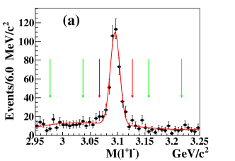
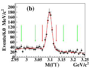
Figure 1: The invariant-mass distributions of the lepton pair from (a) the $\Upsilon(1S)$ data sample and (b) the $\Upsilon(2S)$ data sample. The curves show the best fit results with a Gaussian function for the $J/\psi$ signal and a second-order Chebychev function for the backgrounds. The red arrows indicate the $J/\psi$ signal region and the green ones indicate the $J/\psi$ mass sideband regions.

Figures 2(a) and 2(b) show the distributions of the recoil mass squared against the $pJ/\psi$ system in $\Upsilon(1,2S)$ data samples and signal MC simulations. This quantity is calculated by $M_{\rm recoil}^{2}(pJ/\psi)\equiv(P_{e^{+}e^{-}}-P_{J/\psi})^{2}$, where $P_{e^{+}e^{-}}$ is the 4-momentum of the $e^{+}e^{-}$ collision and $P_{pJ/\psi}$ is the 4-momentum of the $pJ/\psi$ combination. In data, there are accumulations between $-5~{}\hbox{GeV}^{2}/c^{4}$ and $5~{}\hbox{GeV}^{2}/c^{4}$ for the events selected in the $J/\psi$ signal region and these can be described well with the backgrounds estimated from the $J/\psi$ mass sideband regions. These backgrounds appear in the $e^{+}e^{-}$ mode but are scarce in the $\mu^{+}\mu^{-}$ mode. On the other hand, these events produce a large peak at zero and a wide distribution of the recoil mass squared against the $J/\psi$ candidate, calculated by $M_{\rm recoil}^{2}(J/\psi)\equiv(P_{e^{+}e^{-}}-P_{J/\psi})^{2}$, where $P_{J/\psi}$ is the 4-momentum of the $J/\psi$ candidate. They are identified as backgrounds from Bhabha events with high energy bremsstrahlung radiation photon(s) and an additional proton from beam backgrounds. As this proton is not from an $e^{+}e^{-}$ collision, this background can produce negative accumulations in the $M_{\rm recoil}^{2}(pJ/\psi)$ distributions. We require $M_{\rm recoil}^{2}(pJ/\psi)>10~{}\hbox{GeV}^{2}/c^{4}$ to suppress these backgrounds with a selection efficiency of about 99% in $\Upsilon(1,2S)$ decays. Figures 2(c) and 2(d) show the distributions of $M_{\rm recoil}^{2}(J/\psi)$ after this requirement. We notice that the data have higher distributions than signal MC simulations in the region $M_{\rm recoil}^{2}(J/\psi)<30~{}\hbox{GeV}^{2}/c^{4}$. In the range $M_{\rm recoil}^{2}(J/\psi)>30~{}\hbox{GeV}^{2}/c^{4}$, the MC and the data are in good agreement in $\Upsilon(1S)$, but the MC is slightly higher than the data in $\Upsilon(2S)$. It is also interesting to see an enhancement at around $22~{}\hbox{GeV}^{2}/c^{4}$ in the $\Upsilon(1S)$ decays. However, the statistics are too limited to draw any conclusions with the presently available dataset.

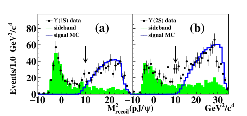
Figure 2: The distributions of the recoil mass squared of $pJ/\psi$ (upper), and $J/\psi$ (lower) in $\Upsilon(1S)$ (left) and $\Upsilon(2S)$ (right) decays. The dots with error bars are data, the shaded histograms are backgrounds estimated from the $J/\psi$ mass sideband regions, and the solid histograms are signal MC simulations. The arrows show the requirement $M_{\rm recoil}^{2}(pJ/\psi)>10~{}{\hbox{GeV}^{2}/c^{4}}$.

IV Invariant mass spectra of $pJ/\psi$

All the candidates satisfying the selection criteria described above are accepted, including $p$ or $\bar{p}$ with the same $J/\psi$ candidate or multiple candidates sharing one lepton. We show the momentum distributions of the $p/\bar{p}$ after selection criteria in Fig. 3.

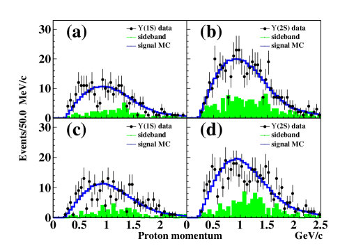
Figure 3: The momentum distributions of $p/\bar{p}$ in $\Upsilon(1,2S)$ inclusive decays. The first row is the momenta of $p$ and the second of $\bar{p}$. The left and right panels are $\Upsilon(1S)$ and $\Upsilon(2S)$, respectively. The dots with error bars are data, the shaded histograms are backgrounds estimated from the $J/\psi$ mass sideband regions, and the solid histograms are signal MC simulations.

According to the efficiency MC simulations, we obtain an efficiency varying from 29% (26%) to 36% (33%) in the $\Upsilon(1S)$ [$\Upsilon(2S)$] decays, and the mass resolution increasing from $1.5~{}\hbox{MeV}/c^{2}$ to $4.9~{}\hbox{MeV}/c^{2}$ for $M_{pJ/\psi}\in[4.1,~{}5.0]~{}\hbox{GeV}/c^{2}$. We notice that the width of $P_{c}(4457)^{+}$ reported by LHCb is $\Gamma_{P_{c}(4457)^{+}}=6.4\pm 2.0^{+5.7}_{-1.9}~{}\hbox{MeV}$ [15] and the mass resolution near the mass of $P_{c}(4457)^{+}$ is about $3.0~{}\hbox{MeV}/c^{2}$. Therefore, we need to consider the mass resolution in fitting the $M_{pJ/\psi}$ distributions for the possible $P_{c}^{+}$ signals. Here and hereinafter, the first uncertainty quoted is statistical, while the second corresponds to the total systematic uncertainty.

We then study the $M_{pJ/\psi}$ distributions from the signal MC simulations of $P_{c}(4312)^{+}$, $P_{c}(4440)^{+}$, and $P_{c}(4457)^{+}$. In each distribution, there is a clear $P_{c}^{+}$ peak and a plateau of wrong combination with particle(s) from the recoil of $P_{c}^{+}$. We perform a fit to this distribution using a Breit-Wigner function convolved with a Gaussian resolution function to describe the signals and a first-order polynomial function to describe the plateau of the wrong combinations. The fit range is $M_{P_{c}^{+}}\pm 200~{}\hbox{MeV}/c^{2}$, where $M_{P_{c}^{+}}$ is the mass of $P_{c}^{+}$. The fits yield mass resolutions of around $3~{}\hbox{MeV}/c^{2}$ for each $P_{c}^{+}$ state. The mass resolutions obtained here agree with those obtained from the efficiency MC simulations directly. We calculate the ratio $\mathcal{R}\equiv N_{P_{c}^{+}}/N_{pJ/\psi}$ to be approximately 0.6, where the $N_{P_{c}^{+}}$ and $N_{pJ/\psi}$ are the number of $P_{c}^{+}$ signals from the fit and the number of all $pJ/\psi$ combinations being selected between $4.0~{}\hbox{GeV}/c^{2}$ and $5.0~{}\hbox{GeV}/c^{2}$, respectively. The efficiencies of all combinations ($\varepsilon^{\rm MC}_{\rm allcmb}$) are about 60%. We list the details of the mass resolutions, the ratios $\mathcal{R}$, and the efficiencies $\varepsilon^{\rm MC}_{\rm allcmb}$ from the signal MC simulations of $P_{c}(4312)^{+}$, $P_{c}(4440)^{+}$, and $P_{c}(4457)^{+}$ in $\Upsilon(1,2S)$ inclusive decays in Table 1.

Table 1: The mass resolution, the ratio of the number of $P_{c}^{+}$ signals to the number of all $pJ/\psi$ combinations, and the efficiency of all the $pJ/\psi$ combinations from the signal MC simulations of $P_{c}(4312)^{+}$, $P_{c}(4440)^{+}$, and $P_{c}(4457)^{+}$ in $\Upsilon(1,2S)$ decays.

	$\Upsilon(1S)$ decays			$\Upsilon(2S)$ decays
—	$P_{c}(4312)^{+}$	$P_{c}(4440)^{+}$	$P_{c}(4457)^{+}$	$P_{c}(4312)^{+}$	$P_{c}(4440)^{+}$	$P_{c}(4457)^{+}$
mass resolution ($\hbox{MeV}/c^{2}$)	$2.9\pm 0.1$	$3.2\pm 0.2$	$3.4\pm 0.1$	$2.8\pm 0.1$	$3.0\pm 0.2$	$3.2\pm 0.1$
Ratio of $N_{P_{c}^{+}}/N_{pJ/\psi}$	0.60	0.56	0.57	0.59	0.56	0.54
$\varepsilon^{\rm MC}_{\rm allcmb}$ (%)	$58.7\pm 0.1$	$59.2\pm 0.1$	$59.7\pm 0.1$	$58.9\pm 0.1$	$59.2\pm 0.1$	$59.5\pm 0.1$

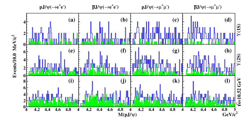
Figure 4: The invariant-mass distributions of $pJ/\psi$ in the $\Upsilon(1S)$, $\Upsilon(2S)$, and continuum data samples. From left to right, the four panels are $p+J/\psi$ in $e^{+}e^{-}$ mode, $\bar{p}+J/\psi$ in $e^{+}e^{-}$ mode, $p+J/\psi$ in $\mu^{+}\mu^{-}$ mode, and $\bar{p}+J/\psi$ in $\mu^{+}\mu^{-}$ mode. From top to bottom, the three rows are the $\Upsilon(1S)$ decays, the $\Upsilon(2S)$ decays, and the continuum productions at $\sqrt{s}=10.52~{}\hbox{GeV}$. The solid histograms are the $pJ/\psi$ signals, and the shaded histograms are backgrounds estimated from the $J/\psi$ mass sideband regions.

We study the $M_{pJ/\psi}$ distributions obtained from the $\Upsilon(1S)$, $\Upsilon(2S)$, and continuum data samples, and show them in Figs. 4(a-d), 4(e-h), and 4(i-l), respectively. There are clear $pJ/\psi$ signals in the three data samples. As mentioned, we use the distributions obtained from the continuum data sample to estimate the backgrounds from $e^{+}e^{-}$ annihilation in the $\Upsilon(1,2S)$ decays. For this, we scale the luminosities and correct for the efficiencies and the c.m. energy dependence of the Quantum Electrodynamics (QED) cross section $\sigma_{e^{+}e^{-}}\propto 1/s$, resulting in scale factors $f_{\rm scale}=(\mathcal{L}_{\Upsilon(1,2S)}\times\varepsilon_{\Upsilon(1,2S)}\times s_{\rm cont})/(\mathcal{L}_{\rm cont}\times\varepsilon_{\rm cont}\times s_{\Upsilon(1,2S)})=0.077$ and 0.301 for $\Upsilon(1S)$ and $\Upsilon(2S)$, respectively. We find no peaking component in the combined $M_{pJ/\psi}$ distribution from Figs 4(i-l) and obtain the number of $pJ/\psi$ candidates to be $N^{pJ/\psi}_{\rm cont}=383\pm 20$ after subtracting the backgrounds estimated from the $J/\psi$ mass sideband regions. To estimate the backgrounds due to the mis-identification of proton, we replace the proton identification requirements with $\mathcal{L}_{p}/(\mathcal{L}_{p}+\mathcal{L}_{K})<0.4$ or $\mathcal{L}_{p}/(\mathcal{L}_{p}+\mathcal{L}_{\pi})<0.4$ in the signal selection. We obtain $1746\pm 42$ $K^{\pm}J/\psi$ signals with kaon identification efficiency of 93.5% or $1710\pm 41$ $\pi^{\pm}J/\psi$ signals with pion identification efficiency of 92.4%. Taking into account mis-identification rates, we expect the number of backgrounds from $K^{\pm}J/\psi$ or $\pi^{\pm}J/\psi$ to be $50.3\pm 0.9\pm 1.3$, where the systematic uncertainty is described in Sec. V. Hence, the number of $pJ/\psi$ events after all background subtractions is found to be $N^{pJ/\psi}_{\rm cont}=333\pm 18$. With the scale factor $f_{\rm scale}$, we expect $26\pm 2\pm 1$ and $100\pm 5\pm 4$ $pJ/\psi$ signals from $e^{+}e^{-}$ annihilation in the $\Upsilon(1S)$ and $\Upsilon(2S)$ data samples, respectively.

We use the $N^{pJ/\psi}_{\rm cont}$ obtained from the continuum data sample to calculate the cross section of the inclusive $pJ/\psi$ production in $e^{+}e^{-}$ annihilation via

$$\sigma(e^{+}e^{-}\to pJ/\psi+anything)=\frac{N^{pJ/\psi}_{\rm cont}}{L_{\rm cont}\times\varepsilon_{\rm cont}^{\rm noP_{c}}\times{\cal B}(J/\psi\to\ell^{+}\ell^{-})\times(1+\delta_{\rm ISR})}.$$ (1)

Here, $\varepsilon_{\rm cont}^{\rm noP_{c}}=66.1\%$ is the efficiency obtained from no-$P_{c}^{+}$ MC simulation of continuum production, $(1+\delta_{\rm ISR})=0.82$ is the radiative correction factor [30, 31], and ${\cal B}(J/\psi\to\ell^{+}\ell^{-})=(11.93\pm 0.07)\%$ is the branching fraction of $J/\psi$ decaying to $e^{+}e^{-}$ or $\mu^{+}\mu^{-}$ [29]. We obtain the cross section $\sigma(e^{+}e^{-}\to pJ/\psi+anything)=(57.5\pm 2.1\pm 2.5)~{}$\mathrm{fb}$$ at $\sqrt{s}=10.52~{}\hbox{GeV}$, where the systematic uncertainties are discussed in Sec. V.

Figure 5 shows the combined distributions of Figs. 4(a-d) and 4(e-h) for $\Upsilon(1S)$ and $\Upsilon(2S)$ inclusive decays, respectively. Since we measure the $pJ/\psi$ production in $\Upsilon(1,2S)$ inclusive decays, the background of continuum production in Fig. 5 is removed. We estimate the number of backgrounds from $K^{\pm}J/\psi$ or $\pi^{\pm}J/\psi$ to be $17.9\pm 1.2$ ($43.9\pm 3.0$) in $\Upsilon(1S)$ [$\Upsilon(2S)$] decays. With the backgrounds estimated from the $J/\psi$ mass sidebands and those from mis-identification of proton being subtracted, we get the final numbers of $pJ/\psi$ signal events to be $N^{pJ/\psi}_{\Upsilon(1S)}=363\pm 19$ in the $\Upsilon(1S)$ decays and $N^{pJ/\psi}_{\Upsilon(2S)}=541\pm 23$ in the $\Upsilon(2S)$ decays. These yields are much higher than those estimated to be due to the underlying $e^{+}e^{-}$ continuum production. To measure the production of $pJ/\psi$ in $\Upsilon(1,2S)$ inclusive decays, we use the no-$P_{c}^{+}$ MC samples to estimate the efficiencies to be $\varepsilon_{\Upsilon(1,2S)}^{\rm noP_{c}}=64.8\%$ and 65.1% for the $\Upsilon(1S)$ and $\Upsilon(2S)$ inclusive decays in the region of $4.0~{}\hbox{GeV}/c^{2}<M_{pJ/\psi}<5.5~{}\hbox{GeV}/c^{2}$. We calculate the branching fractions of $\Upsilon(1,2S)$ inclusive decays using

$${\cal B}[\Upsilon(1,2S)\to pJ/\psi+anything]=\frac{N^{pJ/\psi}_{\Upsilon(1,2S)}-f_{\rm scale}\times N^{pJ/\psi}_{\rm cont}}{N_{\Upsilon(1,2S)}\times\varepsilon_{\Upsilon(1,2S)}^{\rm noPc}\times{\cal B}(J/\psi\to\ell^{+}\ell^{-})},$$ (2)

where $N_{\Upsilon(1,2S)}$ are the numbers of $\Upsilon(1,2S)$ events in the $\Upsilon(1,2S)$ data samples. We obtain that ${\cal B}[\Upsilon(1S)\to pJ/\psi+anything]=(4.27\pm 0.16\pm 0.20)\times 10^{-5}$ and ${\cal B}[\Upsilon(2S)\to pJ/\psi+anything]=(3.59\pm 0.14\pm 0.16)\times 10^{-5}$ for the first time. Excluding the background of $\Upsilon(2S)\to\Upsilon(1S)+anything$ transitions and $\Upsilon(1S)\to pJ/\psi+anything$ with this measurement of ${\cal B}[\Upsilon(1S)\to pJ/\psi+anything]$, we correct the ${\cal B}[\Upsilon(2S)\to pJ/\psi+anything]$ and find a value of $(2.46\pm 0.15\pm 0.17)\times 10^{-5}$. Systematic uncertainties are listed in Table 3, which is described in Sec. V. The world average values of the branching fractions of $J/\psi$ production in $\Upsilon(1,2S)$ decays are ${\cal B}[\Upsilon(1S)\to J/\psi+anything]=(5.4\pm 0.4)\times 10^{-4}$ and ${\cal B}[\Upsilon(2S)\to J/\psi+anything]<6\times 10^{-3}$ at 90% credibility [29]. Thus, the ratio ${\cal B}(\Upsilon\to pJ/\psi+anything)/{\cal B}(\Upsilon\to J/\psi+anything)$ is of order $10^{-1}-10^{-2}$ in $\Upsilon(1,2S)$ decays.

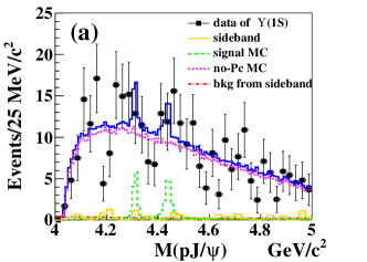
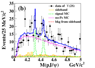
Figure 5: The combined distributions of the invariant masses of $pJ/\psi$ and $\bar{p}J/\psi$ from (a) the $\Upsilon(1S)$ inclusive decays and (b) the $\Upsilon(2S)$ inclusive decays, and the fit results including $P_{c}(4312)^{+}$, $P_{c}(4440)^{+}$ and $P_{c}(4457)^{+}$. The dots with error bars are data. The shaded histograms are the backgrounds estimated from the $J/\psi$ mass sidebands. The blue histograms are the best fit results; the green histograms are the $P_{c}(4312)^{+}$, $P_{c}(4440)^{+}$, and $P_{c}(4457)^{+}$ components; the pink histograms are the no-$P_{c}^{+}$ components.

To estimate the production of a possible $P_{c}^{+}$ state in the $\Upsilon(1S)$ or $\Upsilon(2S)$ inclusive decays, we perform binned maximum likelihood fits to the distribution of $M_{pJ/\psi}$ in Fig. 5(a) or  5(b) with

$$f_{\rm PDF}=f_{P_{c}(4312)^{+}}+f_{P_{c}(4440)^{+}}+f_{P_{c}(4457)^{+}}+f_{\rm noP_{c}}+f_{\rm bkg},$$ (3)

where $f_{P_{c}(4312)^{+}}$, $f_{P_{c}(4440)^{+}}$, $f_{P_{c}(4457)^{+}}$, and $f_{\rm noP_{c}}$ are the histogram PDFs obtained from the signal MC simulations on $P_{c}(4312)^{+}$, $P_{c}(4440)^{+}$, $P_{c}(4457)^{+}$, and the no-$P_{c}^{+}$ MC simulation. We use a second-order polynomial function for the $f_{\rm bkg}$ to describe the backgrounds due to $J/\psi$ selection. We fit to the events from the $J/\psi$ signal region with $f_{\rm PDF}$ and the events from $J/\psi$ mass sidebands with $f_{\rm bkg}$ simultaneously. The fit yields the numbers of $P_{c}^{+}$ signals [$N_{\rm fit}^{\rm A}(P_{c}^{+})$], as listed in Table 2. Since none of the $P_{c}(4312)^{+}$, $P_{c}(4440)^{+}$, or $P_{c}(4457)^{+}$ is significant, we integrate the likelihood versus the $N_{\rm fit}^{\rm A}(P_{c}^{+})$ and determine the upper limits $N_{\rm fit}^{\rm A,UL}(P_{c}^{+})$ at 90% credibility. We also perform a fit to the $M_{pJ/\psi}$ distribution in Fig. 5(a) or  5(b) with individual $P_{c}^{+}$ state in the $f_{\rm PDF}$, which yields the new number of $P_{c}^{+}$ signal [$N_{\rm fit}^{\rm B}(P_{c}^{+})$]. Similarly, we determine the related upper limits $N_{\rm fit}^{\rm B,UL}(P_{c}^{+})$ for $P_{c}(4312)^{+}$, $P_{c}(4440)^{+}$, and $P_{c}(4457)^{+}$ at 90% credibility. We also estimate the upper limits by varying the masses and widths of $P_{c}^{+}$ states by $1\sigma$ in these tests. We take the largest values of the upper limits as the conservative estimations of the upper limits of the numbers of the $P_{c}^{+}$ signals [$N^{\rm UL}_{\rm sig}(P_{c}^{+})$] in $\Upsilon(1,2S)$ inclusive decays. We then calculate the upper limit of the branching fraction of a $P_{c}^{+}$ state produced in $\Upsilon(1S)$ [$\Upsilon(2S)$] inclusive decays at 90% credibility with

$${\cal B}[\Upsilon(1,2S)\to P_{c}^{+}+anything]\cdot{\cal B}(P_{c}^{+}\to pJ/\psi)<\frac{N^{\rm UL}_{\rm sig}(P_{c}^{+})}{N_{\Upsilon(1,2S)}\cdot\varepsilon^{\rm MC}_{\rm allcmb}\cdot{\cal B}(J/\psi\to\ell^{+}\ell^{-})(1-\delta_{\rm sys})},$$ (4)

where $\delta_{\rm sys}=5.0\%~{}(4.7\%)$ is the systematic uncertainty of $\Upsilon(1S)$ [$\Upsilon(2S)$] decays, which are described in Sec. V. We summarize the values of $N_{\rm fit}^{\rm A}(P_{c}^{+})$, $N_{\rm fit}^{\rm A,UL}(P_{c}^{+})$, $N_{\rm fit}^{B}(P_{c}^{+})$, $N_{\rm fit}^{\rm B,UL}(P_{c}^{+})$, $N^{\rm UL}_{\rm sig}(P_{c}^{+})$, and the upper limit of ${\cal B}[\Upsilon(1,2S)\to P_{c}^{+}+anything]\cdot{\cal B}(P_{c}^{+}\to pJ/\psi)$ at 90% credibility in Table 2.

Table 2: The fit results and the upper limits of $P_{c}(4312)^{+}$, $P_{c}(4440)^{+}$, and $P_{c}(4457)^{+}$ productions in $\Upsilon(1,2S)$ inclusive decays. $N_{\rm fit}^{\rm A}$ is the number of $P_{c}^{+}$ signals in the fit with the PDF function $f_{\rm PDF}$ contains $P_{c}(4312)^{+}$, $P_{c}(4440)^{+}$, and $P_{c}(4457)^{+}$ states, and $N_{\rm fit}^{\rm A,UL}$ is the related upper limits at 90% credibility. $N_{\rm fit}^{\rm B}$ is the number of $P_{c}^{+}$ signals in the fit with the PDF function that contains only a single $P_{c}^{+}$ state, and $N_{\rm fit}^{\rm B,UL}$ is the related upper limits at 90% credibility. $N^{\rm UL}_{\rm sig}$ is the final conservative estimation of the upper limit of the number of $P_{c}^{+}$ signals in $\Upsilon(1,2S)$ inclusive decays. ${\cal B}^{\rm UL}$ is the upper limit of ${\cal B}(\Upsilon\to P_{c}^{+}+anything)\cdot{\cal B}(P_{c}^{+}\to pJ/\psi)$ at 90% credibility.

	$\Upsilon(1S)$ decays			$\Upsilon(2S)$ decays
—	$P_{c}(4312)^{+}$	$P_{c}(4440)^{+}$	$P_{c}(4457)^{+}$	$P_{c}(4312)^{+}$	$P_{c}(4440)^{+}$	$P_{c}(4457)^{+}$
$N_{\rm fit}^{\rm A}$	$10\pm 8$	$14\pm 12$	$-3\pm 9$	$30\pm 16$	$33\pm 15$	$0\pm 3$
$N_{\rm fit}^{\rm A,UL}$	26	37	14	52	60	6
$N_{\rm fit}^{\rm B}$	$10\pm 8$	$12\pm 11$	$3\pm 9$	$29\pm 12$	$31\pm 15$	$0\pm 3$
$N_{\rm fit}^{\rm B,UL}$	26	33	17	50	57	7
$N^{\rm UL}_{\rm sig}$	31	47	34	56	77	26
${\cal B}^{\rm UL}$ ($\times 10^{-6}$)	4.5	6.8	4.9	5.3	7.2	2.4

V Systematic uncertainties

Table 3: The summary of the systematic uncertainties (%) in the measurements of ${\cal B}[\Upsilon(1,2S)\to pJ/\psi+anything]$ and $\sigma(e^{+}e^{-}\to pJ/\psi+anything)$ at $\sqrt{s}=10.52~{}\hbox{GeV}$.

Source	$\Upsilon(1S)$ decay	$\Upsilon(2S)$ decay	$\sigma(e^{+}e^{-}\to pJ/\psi+anything)$
Particle identification	2.1	2.1	2.1
Tracking	1.1	1.1	1.1
$J/\psi$ signal region	0.6	0.5	0.4
$M_{\rm recoil}^{2}(pJ/\psi)$ requirement	1.5	1.5	1.5
${\cal B}(J/\psi\to\ell^{+}\ell^{-})$	0.6	0.6	0.6
$1+\delta_{\rm ISR}$	—	—	1.0
Modeling in MC simulation	2.8	2.3	2.6
Number of $\Upsilon(1,2S)$ events	2.2	2.3	—
Integrated luminosity	—	—	1.4
Statistics of MC samples	0.5	0.5	0.5
Sum in quadrature	4.6	4.4	4.3

As listed in Table 3, we consider the following systematic uncertainties in determining the branching fractions ${\cal B}[\Upsilon(1,2S)\to pJ/\psi+anything]$ and measuring $\sigma(e^{+}e^{-}\to pJ/\psi+anything)$ at $\sqrt{s}=10.52~{}\hbox{GeV}$: particle identification, tracking efficiency, $J/\psi$ signal region, $M_{\rm recoil}^{2}(pJ/\psi)$ requirement, branching fraction of $J/\psi$ decay, number of $\Upsilon(1,2S)$ events, integrated luminosity, modeling in MC simulation, and statistics of MC samples, etc. The uncertainties due to the lepton identification are 2.0% and 0.5% for $e^{\pm}$ and $\mu^{\pm}$, respectively. For the proton identification, we have applied an efficiency correction according to the momentum and angle in the laboratory frame. Shifting the correction factor by $1\sigma$, we get the related efficiency difference of 0.43% and take 0.5% to be the systematic uncertainty of proton identification. Therefore, the total systematic uncertainty due to the particle identification is 2.1%. In estimating the backgrounds from $KJ/\psi$ or $\pi J/\psi$, the mis-identification of $K(\pi)$ to $p$ is ($1.98\pm 0.07)\%~{}[(0.72\pm 0.02)\%]$. The uncertainties of mis-identification are not listed in Table 3 but contribute 0.4, 1.1, 1.3 in the numbers of estimated backgrounds from $KJ/\psi$ and $\pi J/\psi$ in $\Upsilon(1S)$ decays, $\Upsilon(2S)$ decays, and continuum productions. The uncertainty due to the tracking efficiency is 0.35% per track and adds linearly. Fitting the $M_{\ell^{+}\ell^{-}}$ distributions from data and MC simulations with a Gaussian function for $J/\psi$ signal and a second-order Chebychev function for backgrounds, we obtain the efficiencies of $J/\psi$ mass signal window to be $\varepsilon^{\rm data}_{J/\psi}=(99.43\pm 0.58)\%$, $(99.56\pm 0.48)\%$, and $(99.69\pm 0.37)$% in $\Upsilon(1S)$ decays, $\Upsilon(2S)$ decays, and continuum productions in data, and $\varepsilon^{\rm MC}_{J/\psi}=99.9\%$ in the signal MC simulations. We correct the efficiencies by the ratios $\varepsilon^{\rm data}_{J/\psi}/\varepsilon^{\rm MC}_{J/\psi}$, and take the errors of the ratios to be the systematic uncertainties, i.e., 0.6% in the $\Upsilon(1S)$ decays, 0.5% in the $\Upsilon(2S)$ decays and 0.4% in the continuum productions. The efficiencies of the requirement $M_{\rm recoil}^{2}(pJ/\psi)>10~{}\hbox{GeV}^{2}/c^{4}$ are 98.9%, 99.9%, and 99.9% in signal MC simulations for the $\Upsilon(1S)$ decays, the $\Upsilon(2S)$ decays, and the continuum productions. Since all the MC simulations of the $P_{c}^{+}$ decay model and no-$P_{c}^{+}$ process show efficiencies higher than 98.5%, we take 1.5% as the systematic uncertainty of the requirement on $M_{\rm recoil}^{2}(pJ/\psi)$. According to the world average values [29], ${\cal B}(J/\psi\to\ell^{+}\ell^{-})(l=e,\mu)$ contributes a systematic uncertainty of 0.6%. By varying the photon energy cutoff by $50~{}\hbox{MeV}$ in the simulation of ISR, we determine the change of $1+\delta_{\rm ISR}$ to be 0.01 and take 1.0% to be the conservative systematic uncertainty in measuring the cross section $\sigma(e^{+}e^{-}\to pJ/\psi+anything)$ at $\sqrt{s}=10.52~{}\hbox{GeV}$. There are uncertainties in modeling the final states in the MC simulations. In the hadronization of $q\bar{q}$, we vary the mass and width of $X$ by $200~{}\hbox{MeV}/c^{2}$ and $500~{}\hbox{MeV}$, which have differences in efficiency that 2.6% in the $\Upsilon(1S)$ decays, 1.9% in the $\Upsilon(2S)$ decays and 2.3% in the continuum production, respectively. Considering that the proton candidate may come from $\Lambda$ decay, we simulate the MC samples of $\Upsilon(1,2S)\to pJ/\psi+\bar{\Lambda}+(s\bar{q})$ and find the efficiency differences, from those of $P_{c}^{+}$ signal MC samples, of 1.1% in $\Upsilon(1S)$ decays, 1.2% in $\Upsilon(2S)$ decays, and 1.1% in contnuum production. We sum the two sources and obtain the systematic uncertainties in modeling the final states in MC simulations to be to be 2.8%, 2.3%, and 2.6% in $\Upsilon(1S)$ decays, $\Upsilon(2S)$ decays, and continuum productions at $\sqrt{s}=10.52~{}\hbox{GeV}$. The uncertainties of the total numbers of $\Upsilon(1S)$ events and $\Upsilon(2S)$ events are 2.2% and 2.3% in the Belle data samples [20, 21]. The common uncertainty in the integrated luminosities for the $\Upsilon(1S)$, $\Upsilon(2S)$, and continuum data samples is 1.4%, which is canceled in calculating the scale factor $f_{\rm scale}$. The statistical uncertainties of the signal MC samples are 0.5% in common. Assuming these uncertainties are independent and sum them in quadrature, we obtain the total systematic uncertainties to be 4.6% in ${\cal B}[\Upsilon(1S)\to pJ/\psi+anything]$, 4.4% in ${\cal B}[\Upsilon(2S)\to pJ/\psi+anything]$, and 4.3% in $\sigma(e^{+}e^{-}\to pJ/\psi+anything)$ at $\sqrt{s}=10.52~{}\hbox{GeV}$.

In determining the upper limits of $P_{c}^{+}$ productions in $\Upsilon(1,2S)$ decays, most of the systematic uncertainties are the same as those listed in Table 3, with the exception of the modeling of $pJ/\psi$ in signal MC simulations and additional uncertainties in fits. To evaluate these, we do the similar studies, including varying the mass and width of $X\to q\bar{q}$ and simulating the MC sample of $\Upsilon(1,2S)\to P_{c}^{+}+\bar{\Lambda}+(s~{}\bar{q})$. We replace the uncertainties in modeling by 3.3% in $\Upsilon(1S)$ decays and 2.9% in $\Upsilon(2S)$ decays in Table 3. Therefore, the total systematic uncertainties of $P_{c}^{+}$ productions in $\Upsilon(1S)$ decays and $\Upsilon(2S)$ decays are 5.0% and 4.7%, respectively. To estimate the systematic uncertainty of $f_{\rm noP_{c}}$ in the fits, we investigate the difference in the yield when using an ARGUS function to replace the histogram PDF obtained from the no-$P_{c}^{+}$ MC simulation [32]. We change the masses and the widths of the $P_{c}^{+}$ states by $1\sigma$ according to LHCb measurement [15]. As before, we take the highest values of $N^{\rm UL}_{\rm sig}(P_{c}^{+})$ to calculate the upper limit of $P_{c}^{+}$ production in the $\Upsilon(1,2S)$ inclusive decays.

VI Summary

We study the $pJ/\psi$ final states in $\Upsilon(1,2S)$ inclusive decays and search for the $P_{c}(4312)^{+}$, $P_{c}(4440)^{+}$ and $P_{c}(4457)^{+}$ signals. To study the production of $pJ/\psi$ in the $\Upsilon(1,2S)$ data samples, we also investigate the $pJ/\psi$ final state in the Belle continuum data sample. We determine the branching fractions to be ${\cal B}[\Upsilon(1S)\to pJ/\psi+anything]=(4.27\pm 0.16\pm 0.20)\times 10^{-5}$ and ${\cal B}[\Upsilon(2S)\to pJ/\psi+anything]=(3.59\pm 0.14\pm 0.16)\times 10^{-5}$, and the cross section of continuum production to be $\sigma(e^{+}e^{-}\to pJ/\psi+anything)=(57.5\pm 2.1\pm 2.5)~{}$\mathrm{fb}$$ at $\sqrt{s}=10.52~{}\hbox{GeV}$. No significant $P_{c}^{+}$ signals exist in the Belle $\Upsilon(1,2S)$ data samples. We determine the upper limits of $P_{c}^{+}$ productions in $\Upsilon(1,2S)$ inclusive decays to be

$${\cal B}[\Upsilon(1S)\to P_{c}(4312)^{+}+anything]\cdot{\cal B}[P_{c}(4312)^{+}\to pJ/\psi] < 4.5\times 10^{-6},$$ (5)

$${\cal B}[\Upsilon(1S)\to P_{c}(4440)^{+}+anything]\cdot{\cal B}[P_{c}(4440)^{+}\to pJ/\psi] < 6.8\times 10^{-6},$$ (6)

$${\cal B}[\Upsilon(1S)\to P_{c}(4457)^{+}+anything]\cdot{\cal B}[P_{c}(4457)^{+}\to pJ/\psi] < 4.9\times 10^{-6},$$ (7)

$${\cal B}[\Upsilon(2S)\to P_{c}(4312)^{+}+anything]\cdot{\cal B}[P_{c}(4312)^{+}\to pJ/\psi] < 5.3\times 10^{-6},$$ (8)

$${\cal B}[\Upsilon(2S)\to P_{c}(4440)^{+}+anything]\cdot{\cal B}[P_{c}(4440)^{+}\to pJ/\psi] < 7.2\times 10^{-6},$$ (9)

$${\cal B}[\Upsilon(2S)\to P_{c}(4457)^{+}+anything]\cdot{\cal B}[P_{c}(4457)^{+}\to pJ/\psi] < 2.4\times 10^{-6},$$ (10)

at 90% credibility.

References

[1] M. Gell-Mann,
Phys. Lett. 8, 214 (1964).
[2] N. Brambilla et al.,
Eur. Phys. J. C 71, 1534 (2011).
[3] S. L. Olsen, T. Skwarnicki and D. Zieminska,
Rev. Mod. Phys. 90, 015003 (2018).
[4] S. K. Choi et al. (Belle Collaboration),
Phys. Rev. Lett. 91, 262001 (2003).
[5] S. K. Choi et al. (Belle Collaboration),
Phys. Rev. Lett. 100, 142001 (2008).
[6] R. Aaij et al. (LHCb Collaboration),
Phys. Rev. Lett. 112, 222002 (2014).
[7] R. Mizuk et al. (Belle Collaboration),
Phys. Rev. D 78, 072004 (2008).
[8] A. Bondar et al. (Belle Collaboration),
Phys. Rev. Lett. 108, 122001 (2012).
[9] M. Ablikim et al. (BESIII Collaboration),
Phys. Rev. Lett. 110, 252001 (2013).
[10] Z. Q. Liu et al. (Belle Collaboration),
Phys. Rev. Lett. 110, 252002 (2013).
[11] M. Ablikim et al. (BESIII Collaboration),
Phys. Rev. Lett. 111, 242001 (2013).
[12] X. L. Wang et al. (Belle Collaboration),
Phys. Rev. D 91, 112007 (2015).
[13] M. Ablikim et al. (BESIII Collaboration),
Phys. Rev. D 96, 032004 (2017).
[14] R. Aaij et al. (LHCb Collaboration),
Phys. Rev. Lett. 115, 072001 (2015).
[15] R. Aaij et al. (LHCb Collaboration),
Phys. Rev. Lett. 122, 222001 (2019).
[16] C. E. Carlson, J. R. Hiller and R. J. Holt,
Annu. Rev. Nucl. Part. Sci. 47, 395 (1997).
[17] D. M. Asner et al. (CLEO Collaboration),
Phys. Rev. D 75, 012009 (2007).
[18] H. Albrecht et al. (ARGUS Collaboration),
Phys. Lett. B 236, 102 (1990).
[19] J. P. Lees et al. (BABAR Collaboration),
Phys. Rev. D 89, 111102(R) (2014).
[20] C. P. Shen et al. (Belle Collaboration),
Phys. Rev. D 82, 051504 (2010).
[21] X. L. Wang et al. (Belle Collaboration),
Phys. Rev. D 84, 071107 (2011).
[22] A. Abashian et al. (Belle Collaboration),
Nucl. Instrum. Methods A 479, 117 (2002); also see detector section in J. Brodzicka et al.,
Prog. Theor. Exp. Phys. 2012, 04D001 (2012).
[23] D. J. Lange,
Nucl. Instrum. Methods A 462, 152 (2001).
[24] T. Sjostrand, S. Mrenna, and P. Skands,
J. High Energy Phys. 05, 026 (2006).
[25] R. Brun et al.,
GEANT 3.21, CERN DD/EE/84-1, 1984.
[26] E. Nakano,
Nucl. Instrum. Methods A 494, 402 (2002).
[27] K. Hanagaki et al.,
Nucl. Instrum. Methods A 485, 490 (2002).
[28] A. Abashian et al.,
Nucl. Instrum. Methods A 491, 69 (2002).
[29] R. L. Workman et al. (Particle Data Group),
Prog. Theor. Exp. Phys. 2022083C012022 and 2023 update.
[30] S. Actis et al.,
Eur. Phys. J. C 66, 585 (2010).
[31] X. K. Dong, X. H. Mo, P. Wang, and C. Z. Yuan,
Chin. Phys. C 44, 083001 (2020).
[32] H. Albrecht et al. (ARGUS Collaboration),
Phys. Lett. B 241, 278 (1990).