A mechanism-informed reinforcement learning framework for shape optimization of airfoils

Abstract

In this study, we present the mechanism-informed reinforcement learning framework for airfoil shape optimization. By leveraging the twin delayed deep deterministic policy gradient algorithm for its notable stability, our approach addresses the complexities of optimizing shapes governed by fluid dynamics. The PDEs-based solver is adopted for its accuracy even when the configurations and geometries are extraordinarily changed during the exploration. Dual-weighted residual-based mesh refinement strategy is applied to ensure the accurate calculation of target functionals. To streamline the iterative optimization process and handle geometric deformations, our approach integrates Laplacian smoothing, adaptive refinement, and a Bézier fitting strategy. This combination not only remits mesh tangling but also guarantees a precise manipulation of the airfoil geometry. Our neural network architecture leverages Bézier curves for efficient dimensionality reduction, thereby enhancing the learning process and ensuring the geometric accuracy of the airfoil shapes. An attention mechanism is embedded within the network to calculate potential action on the state as well. Furthermore, we have introduced different reward and penalty mechanisms tailored to the specific challenges of airfoil optimization. This algorithm is designed to support the optimization task, facilitating a more targeted and effective approach for airfoil shape optimization.

Keywords PDEs-based optimization $\cdot$ Reinforcement learning  $\cdot$ DWR-based adaptation  $\cdot$ Newton-GMG solver  $\cdot$ Mesh smoothing

1 Introduction

Aerodynamic design has been an important research theme for decades, particularly in the context of optimizing airfoils for enhanced aerodynamic performance[1, 2] and fuel efficiency[3]. Multidisciplinary analysis and optimization plays an indispensable part in these fields. Nonetheless, it is pointed out by an important proposal from NASA [4] that high-fidelity computational fluid dynamics(CFD) is not routinely used in this area. Both academia and industry anticipate significant advancements in the integration of CFD methodologies by the year 2030. Aiming at conducting shape optimization of airfoils based on a high-fidelity CFD solver with the state-of-art technique, a mechanism-informed reinforcement learning framework is proposed in this paper.

Classical methods, such as gradient-based techniques[5], genetic algorithms[6] can be adopted to support the optimization task. The traditional method pioneered by Jameson [7, 8] combined the optimization problem with adjoint equations which has been proven to be very efficient. However, the analysis and application of optimization techniques in the industry can not be generalized to more complicated target functional easily[4]. Combining CFD methods with optimization offers some distinct advantages. For instance, a more precise depiction of flow fields enables a more accurate calculation of target functionals. The advent of techniques such as the dual-weighted residual(DWR)-based mesh adaptation[9, 10, 11] allows for the attainment of more precise target functionals while preserving computational accuracy. Moreover, the enhanced coupling between more accurate geometric representations and PDEs provides superior tools for simulating airfoil geometric deformations through the use of parametric curves and unstructured mesh methods to describe shapes[12, 13]. However, PDEs-based optimization also presents various challenges. These include the high computational cost associated with solving PDEs[14] with complex geometries, non-linearities inherent in many physical systems, and application issues for ensuring that optimized shapes are physically realizable[15]. Despite these obstacles, the benefits of PDEs-based approaches such as their precision and robustness, make the technique a powerful tool in the shape optimization domain.

With the development of artificial intelligence in recent years, associating the neural networks with traditional computational fluid dynamics problems becomes feasible in shape optimization of airfoil[16]. In recent years, researchers have been exploring the integration of machine learning into the domain of shape optimization. For example, the Bézier-GAN developed in [17, 18], has been utilized to parameterize aerodynamic designs by learning from shape variations. Similarly, the conditional variational autoencoder [19] has been employed to dissect the intricate relationship between the aerodynamic performance and the shape of airfoils. Moreover, the recent advancements in reinforcement methodologies, such as deep reinforcement learning[20], have significantly expanded its applicability and effectiveness in handling high-dimensional state and action spaces, which provide a basis for the PDEs-based optimization problems.

The distinctive advantages of reinforcement learning, compared with other machine learning algorithms, lie in its ability to make sequential decisions and learn optimal policies directly from interaction with the environment[21]. This is especially pertinent in the realm of control problems governed by partial differential equations[22, 23], where the dynamics are complex and highly nonlinear. Unlike traditional machine learning approaches that often require labeled data sets for training, reinforcement learning thrives in an exploration-based learning environment, making it uniquely suited for optimizing shapes and controls in PDEs-driven systems without the need for extensive pre-processed data. These developments, combined with our group’s work in exploring advanced PDE solvers[24, 25, 26, 12], have laid the groundwork for implementing a PDE solver-based reinforcement learning framework.

Even though reinforcement learning has made significant strides in various applications, its integration into shape optimization, particularly within the context of PDEs-based systems, remains nascent. Ever since in [27], reinforcement learning has been applied to morphing within an airfoil design context. Initially, the application was constrained by the consideration of only four variables for airfoil morphing, primarily due to the extensive time demands of the learning process. With the advent of computational advancements, a direct shape optimization methodology utilizing reinforcement learning was introduced in [28]. However, the number of parameters is still far from the application. Given that computational fluid dynamics solver operations significantly consume CPU time, [29] implemented a transfer learning technique to expedite the learning process. In our research[30, 31, 32], we have integrated the DWR-based mesh refinement strategy, a method that can generate a high quality mesh for the calculation of target functional. With the corresponding parallelization module constructed to accelerate the calculation process[33], our PDE solver can deal with the reinforcement learning process where thousands of airfoil shapes should be taken into consideration.

However, embarking on a shape optimization methodology based on a precise PDE solver, particularly within an unstructured mesh presents additional challenges as follows. i). Automating the iterative process of the entire algorithm, which is highlighted in [34, 35]. During the iterative process of reinforcement learning, the PDE solver might be invoked thousands of times. Manual intervention at each iteration is impractical. However, an automated strategy necessitates a profound understanding of the parameters and robustness throughout the iterative process. This means that even with significant changes in configuration and geometry, the simulation should remain effective. ii). Managing geometric deformations on unstructured meshes, which encompasses potential mesh tangling issues[36]. Mesh deformation is significant for the shape optimization problem, especially for the design of airfoil where the physical properties of the fluid medium are significantly influenced by the geometry of the computational domain. The process of mesh deformation entails the manipulation of mesh nodes and elements to accurately represent the geometry and to facilitate the resolution of complex physical phenomena with high precision. Even though meshless techniques[37] can be adopted, mesh-based approaches still hold a predominant position due to their rigorous theoretical analysis and more advanced method for calculating target functional[38]. However, the deformation on the unstructured meshes is not straightforward because the elements are sensitive to the movement of the boundary that depicts the airfoil. The change of geometry may be stochastic initially, where the quality of meshes can not be guaranteed. Besides, the curvature may change rapidly along the deformed shape. If the curvature variation occurs within the elements, it is challenging to capture the geometry correctly. iii). Tackling the challenges posed by controlling geometries with a large number of parameters, including their geometric representation and the control of high-dimensional parameters for reinforcement learning[39, 40]. The primary difficulty with a high parameter count is that it complicates the simulation process. Furthermore, while a more precise control over geometry enhances manipulability, it also poses challenges to maintaining a cohesive global shape. Excessive control points can lead to issues with the smoothness of curves, which in turn, impacts the reinforcement learning algorithms. For instance, even if the deformation trend is correct, the lack of geometric smoothness can negatively influence the agent’s strategy, potentially leading to the failure of policy iteration. iv). Developing a framework capable of addressing different optimization objectives. The effectiveness of DWR-based mesh adaptation methods is inherently related to the current state of theoretical advancements[9]. The challenge is further compounded when dealing with more complex target functionals, whose resolution poses significant difficulties. Furthermore, translating traditional optimization problems into reinforcement learning frameworks introduces additional complexities. Ensuring the equivalence of primal optimization objectives and the result of reinforcement learning is paramount. This requires the understanding of the reward function[41], necessitating it to be closely compatible with the underlying optimization context.

In this paper, we proposed a novel framework, the mechanism-informed reinforcement learning, for conducting the shape optimization design of airfoils. The problems mentioned above are addressed with techniques as follows. Firstly, in addressing the challenges of automation, the principal difficulty in coupling our framework with current DWR-based mesh adaptation PDE solvers lies in the automatic selection of appropriate tolerance values. These values guide the mesh refinement process across different geometries. In [33], we introduced an algorithm that is capable of dealing with such issues. It not only facilitates automation which is crucial for iterative optimization, but also conserves time while maintaining accuracy. Implementation has been realized within AFVM4CFD, a C++ library maintained by our group. Subsequently, for the deformation of airfoils, we employed Python scripts to interface with the underlying library, facilitating the collection of critical reinforcement learning metrics such as states, actions, and rewards.

Secondly, to address potential mesh tangling issues during the airfoil deformation process, we employed a Laplacian smoothing technique to restore mesh quality after each deformation. Typically, once mesh entanglement has occurred, it is not feasible to rectify the mesh to its optimal state using such methods. On one hand, the restoration process after each deformation helps prevent the accumulation of irregular triangles, significantly reducing the possibility of mesh tangling issues. On the other hand, from the perspective of finite element analysis, irregular triangles of unstructured meshes can introduce additional errors. To manipulate the geometry with more elaborate actions, we utilized over 200 sample points to represent the shape. However, for tensors denoting the shape with such dimensions, local point movements represent a minor modification to the tensors, making it challenging for algorithms to discern significant differences before and after deformation. We introduced a smoothing movement process, ensuring that sample points near the moving point adjust according to this trend. It amplifies the difference between tensors. Additionally, this process also plays a non-negligible role in mitigating mesh tangling. When mesh deformation occurs within the initial mesh simulation dimensions, we employ an adaptive refinement process to capture those elements with a larger geometric change. With such an adaptive refinement method, we are able to capture subtle curvature changes smaller than the mesh size.

Thirdly, to avoid the jagged structures caused by numerous minor curvature changes, we added an additional regularization correction to the process of generating control points from sample points. The control points are restricted to have as equidistant intervals as possible, which significantly makes the shape smoother. Furthermore, the process of generating control points through Bezier fitting serves as an efficient means of dimensionality reduction, allowing for finer geometric control. This also aids the stability of the learning process by facilitating dimensionality reduction.

Last but not least, in order to develop a framework suitable for tackling control problems of this nature, identifying an appropriate reinforcement learning algorithm is essential. We chose the Twin Delayed Deep Deterministic Policy Gradient (TD3) algorithm for stability on continuous optimization problems. The algorithm should be carefully designed as shape optimal design problem can be highly non-linear and sensitive to action parameters. In terms of neural network design, the initial step involves the comprehensive extraction of airfoil shape features. To this end, we employed various techniques, including feature enhancement and leveraging the intrinsic physical properties of geometric points, such as thickness and curvature, to bolster understanding of geometry. Although we experimented with using Variational Autoencoders (VAEs) for feature extraction, the challenges associated with learning an appropriate shape in a high-dimensional space became evident. Consequently, utilizing Bézier curves to reduce dimensionality to a finite set of control points emerged as a more effective representation method. We incorporated specific mapping functions into the action parameters output by the actor network, acknowledging the geometric significance of actual action variations. However, this approach risked potential gradient vanishing issues. Therefore, the actor network was designed not to be overly deep, further underscoring the importance of dimensionality reduction. Techniques such as residual connections[42], the SELU activation function[43], and real-time monitoring via TensorBoard[44] were employed to mitigate and monitor potential gradient vanishing problems. The design of the critic network had to account for the potential impact of actions and their parameters on the high-dimensional state. Hence, the attention mechanism proved to be an effective tool for achieving this goal. For gradient updates, we sampled from the replay buffer, selecting the best historical data, those closest to the current moment, and a weighted random assortment to facilitate policy updates. This approach aids in navigating the optimization landscape more effectively by emphasizing the exploration of promising regions while avoiding local optima. The reward function design emanates from the original optimization problem, aligned with the existing learning framework to define an appropriate reward structure. In the execution phase, we focused on encouraging behaviors associated with higher rewards and penalizing actions that violate constraints, alongside employing empirical exploration strategies. These measures ensure a more efficient iterative process of the algorithm, guiding the learning towards fulfilling the optimization objectives effectively.

The rest of this paper is organized as follows. In Section 2, we briefly introduced the fundamental notations and provided a concise introduction to the Newton-GMG solver. In Section 3, the architecture of our automatic DWR-based mesh adaptation method is introduced. In Section 4, the challenge of mesh deformation within the unstructured mesh is discussed and the recovering method is developed. In section 5, the algorithm of the reinforcement learning, Twin Delayed DDPG is constructed. In Section 6, we conduct the optimization task and present the numerical results.

2 A breif review of Newton-GMG framework

To embark on research involving shape optimization through reinforcement learning, it’s imperative to have a suitable set of governing equations at our disposal. These equations help us understand the distribution of specific physical quantities across space, thereby enabling the precise calculation of the objective functional targeted for optimization. In our previous works [31, 30, 25], we have developed a solver capable of handling the steady Euler equations. This solver not only facilitates the computation of these equations but also ensures the accurate resolution of the target functional, laying a solid foundation for our shape optimization endeavors. A brief introduction will be given in this section.

2.1 Basic notations and finite volume discretization

The steady Euler equations form the backbone of our understanding of inviscid flow behavior and are capable of dealing with the shape optimal design problem[45]. These equations, represented in a conservative form for the inviscid two-dimensional steady state,

$$\nabla\cdot\mathcal{F}(\mathbf{u})=0,\qquad\textbf{in }\Omega.$$ (1)

Here $\mathbf{u}$ and $\mathcal{F}(\mathbf{u})$ are the conservative variables and fluxes, which are given by

$$\mathbf{u}=\begin{bmatrix}\rho\\ \rho u_{x}\\ \rho u_{y}\\ E\end{bmatrix},\quad\text{and}\quad\mathcal{F}(\mathbf{u})=\begin{bmatrix}\rho u_{x}&\rho u_{y}\\ \rho u_{x}^{2}+p&\rho u_{x}u_{y}\\ \rho u_{x}u_{y}&\rho u_{y}^{2}+p\\ u_{x}(E+p)&u_{y}(E+p)\end{bmatrix},$$ (2)

where the terms $(u_{x},u_{y})^{T}$, $\rho$, $p$, and $E$ represent the velocity, density, pressure, and total energy, respectively. The system is completed with the equation of state for an ideal gas, defined as

$$E=\frac{p}{\gamma-1}+\frac{1}{2}\rho(u_{x}^{2}+u_{y}^{2}),$$ (3)

where $\gamma=1.4$ indicates the specific heat ratio.

To address these equations numerically, we turn our focus to discretizing the domain $\Omega$. Consider $\Omega$ as a domain in $\mathbb{R}^{2}$ with boundary denoted by $\Gamma$. We divide $\Omega$ into distinct control volumes, $K_{i}$, via a shape-regular subdivision. Then the mesh under the current mesh size is denoted as $\mathcal{K}_{h}$. Each control volume is referred to as $K_{i}$. The intersection between any two elements $K_{i}$ and $K_{j}$, is labeled as $e_{i,j}$, satisfying $e_{i,j}=\partial K_{i}\cap\partial K_{j}$. The edge $e_{i,j}$ relative to $K_{i}$ is equipped with a unit outer normal vector, $n_{i,j}$.

This setup allows us to redefine the weak form of Euler equations for the discretized domain through the divergence theorem as:

$$\mathcal{A}(\mathbf{u})=\int_{\Omega}\nabla\cdot\mathcal{F}(\mathbf{u})dx=\sum_{i}\int_{K_{i}}\nabla\cdot\mathcal{F}(\mathbf{u})dx=\sum_{i}\sum_{j}\oint_{e_{i,j}\in\partial K_{i}}\mathcal{F}(\mathbf{u})\cdot n_{i,j}ds=0.$$ (4)

To further advance towards a fully discretized system, we introduce a numerical flux function $\mathcal{H}(\cdot,\cdot,\cdot)$, given by:

$$\sum_{i}\sum_{j}\oint_{e_{i,j}\in\partial K_{i}}\mathcal{H}(\mathbf{u}_{i},\mathbf{u}_{j},n_{i,j})ds=0.$$ (5)

2.2 Newton-GMG solver

To tackle the nonlinear Equation (5), we employ the Newton method for linearization, supplemented by a linear multigrid method for solving the equations as proposed in [46]. Initially, we expand Equation (5) using the Taylor series and neglect higher-order terms, simplifying the equations to:

$$\alpha\left|\!\left|\sum\limits_{i}\sum\limits_{j}\int_{e_{i,j}\in\partial\mathcal{K}_{i}}\mathcal{H}(\mathbf{u}_{i}^{(n)},\mathbf{u}_{j}^{(n)},n_{i,j})ds\right|\!\right|_{L_{1}}\Delta\mathbf{u}_{i}^{(n)} +\sum\limits_{i}\sum\limits_{j}\int_{e_{i,j}\in\partial\mathcal{K}_{i}}\Delta\mathbf{u}_{i}^{(n)}\frac{\partial\mathcal{H}(\mathbf{u}_{i}^{(n)},\mathbf{u}_{j}^{(n)},n_{i,j})}{\partial\mathbf{u}_{i}^{(n)}}ds$$ (6)

$$+\sum\limits_{i}\sum\limits_{j}\int_{e_{i,j}\in\partial\mathcal{K}_{i}}\Delta\mathbf{u}_{j}^{(n)}\frac{\partial\mathcal{H}(\mathbf{u}_{i}^{(n)},\mathbf{u}_{j}^{(n)},n_{i,j})}{\partial\mathbf{u}_{j}^{(n)}}ds$$

$$=-\sum\limits_{i}\sum\limits_{j}\int_{e_{i,j}\in\partial\mathcal{K}_{i}}\mathcal{H}(\mathbf{u}_{i}^{(n)},\mathbf{u}_{j}^{(n)},n_{i,j})ds,$$

where $\frac{\partial\mathcal{H}(\cdot,\cdot,\cdot)}{\partial\mathbf{u}}$ represents the Jacobian matrix of the numerical flux, and $\Delta\mathbf{u}_{i}$ represents the increment of conservative variables for the $i$-th element. Following each Newton iteration, the cell average undergoes an update, $\mathbf{u}_{i}^{(n+1)}=\mathbf{u}_{i}^{(n)}+\Delta\mathbf{u}_{i}^{(n)}$.

A regularization term is incorporated into the simulation to enhance system stability. Initially, the solution substantially deviates from a steady state, but as iterations advance, it converges towards equilibrium, reducing the regularization term to near-zero.

Figure 1: Mesh around the NACA0012 airfoil.

For solving Equation (6), the geometric multigrid technique is adopted. As demonstrated in [32], applying regularization and geometric multigrid methods to both primal and dual equations significantly enhances solver robustness, ensuring reliable dual equation resolution.

Figure 2: Mesh around the NACA0012 airfoil. Left: the residual-based mesh adaptation. Right: the DWR-based mesh adaptation.

3 Automatic DWR-based adaptation for the target functional

In our work as discussed in [30, 32], we elaborated on a framework innovated by Darmofal [47], which showcases a fully discrete adjoint-weighted residual technique. This approach was further extended to address two-dimensional inviscid flow scenarios as depicted in [48]. To incorporate this technique within our framework, we present an overview of the methodology.

We denote solutions on the coarse mesh as $\mathbf{u}_{H}$ and on the finer mesh as $\mathbf{u}_{h}$. The initial goal was to precisely compute the numerical integration of $J(\mathbf{u})$ over a fine mesh, denoted as $J_{h}(\mathbf{u}_{h})$ which needs to be solved on the fine mesh directly. Subsequently, to develop the extrapolation method that can calculate this value from the coarse mesh, a multi-variable Taylor series expansion method is adopted as follows:

$$J_{h}(\mathbf{u}_{h})=J_{h}(\mathbf{u}_{h}^{H})+\left.\frac{\partial J_{h}}{\partial\mathbf{u}_{h}}\right|_{\mathbf{u}_{h}^{H}}(\mathbf{u}_{h}-\mathbf{u}_{h}^{H})+\cdots,$$ (7)

where $\mathbf{u}_{h}^{H}$ denotes the coarse mesh solution $\mathbf{u}_{H}$ projected onto the fine mesh space $\mathcal{V}_{h}$ through a prolongation operator $I_{h}^{H}$,

$$\mathbf{u}_{h}^{H}=I_{h}^{H}\mathbf{u}_{H}.$$ (8)

We identify the residual of primal problem in the space $\mathcal{V}_{h}$ by $\mathcal{R}_{h}(\cdot)$, which is expected to satisfy the equations with solution $\mathbf{u}_{h}$, i.e.,

$$\mathcal{R}_{h}(\mathbf{u}_{h})=0.$$ (9)

Upon linearizing, we derive the following expression,

$$\mathcal{R}_{h}(\mathbf{u}_{h})=\mathcal{R}_{h}(\mathbf{u}_{h}^{H})+\left.\frac{\partial\mathcal{R}_{h}}{\partial\mathbf{u}_{h}}\right|_{\mathbf{u}_{h}^{H}}(\mathbf{u}_{h}-\mathbf{u}_{h}^{H})+\cdots.$$ (10)

Given $\left.({\partial\mathcal{R}_{h}}/{\partial\mathbf{u}_{h}})\right|_{\mathbf{u}_{h}^{H}}$ represents the Jacobian matrix, its inversion approximates the error vector as,

$$\mathbf{u}_{h}-\mathbf{u}_{h}^{H}\approx-\left(\left.\frac{\partial\mathcal{R}_{h}}{\partial\mathbf{u}_{h}}\right|_{\mathbf{u}_{h}^{H}}\right)^{-1}\mathcal{R}_{h}(\mathbf{u}_{h}^{H}).$$ (11)

Substituting the error vector into the residual equation yields the updated quantity of interest,

$$J_{h}(\mathbf{u}_{h})=J_{h}(\mathbf{u}_{h}^{H})-(\mathbf{z}_{h}|_{\mathbf{u}_{h}^{H}})^{T}\mathcal{R}_{h}(\mathbf{u}_{h}^{H}),$$ (12)

where $\mathbf{z}_{h}|_{\mathbf{u}_{h}^{H}}$ is derived from the fully discrete dual equations:

$$\left(\left.\frac{\partial\mathcal{R}_{h}}{\partial\mathbf{u}_{h}}\right|_{\mathbf{u}_{h}^{H}}\right)^{T}\mathbf{z}_{h}|_{\mathbf{u}_{h}^{H}}=\left(\left.\frac{\partial J_{h}}{\partial\mathbf{u}_{h}}\right|_{\mathbf{u}_{h}^{H}}\right)^{T}.$$ (13)

The calculation of $\mathbf{z}_{h}$ on the embedded mesh was normally expensive. The literature presents various methods to streamline this process. For instance, the works of [47, 49] introduce an error correction method that interpolates dual solutions onto a fine mesh, while [50] proposes a smoothing technique to mitigate oscillations stemming from interpolation. In recent years, the BiCG method in [10, 51] has been adopted to calculate the dual and primal problems at once. With the help of machine learning techniques, we developed the hybrid CNNs-Dual framework[33] to accelerate the calculation of dual solutions which is very effective. However, the CNNs-Dual solver can not preserve the accuracy for deformed geometry. While techniques like GCN(Graph Convolutional Networks)-enhanced learning should be developed to mend this issue, a conventional algorithm for the DWR-based adaptation is adopted here to calculate the target functional.

Even though the dual solutions can be solved effectively, issues persist on how to balance the value of primal residuals and dual solutions as their magnitudes are not compatible. Indicators for each element are generated based on their multiplication, i.e.,

$$\eta_{K_{i}}=\sum_{K_{ij}}|(\mathbf{z}_{h})^{T}\mathcal{R}_{h}(\mathbf{u}_{h}^{H})|,$$ (14)

where $K_{ij}$ is the subelements $K_{i}$. For the implementation of mesh adaptation, a parameter needs to be set for guiding such a process. However, setting this parameter is tricky because a lower value may lead to an approximately uniform refinement while a higher value may not solve the target functional with expected accuracy. What makes it worse is that such a parameter differs with the update of configurations and different geometries. Thus, it is crucial to find an automatic parameter-setting strategy for guaranteeing the mesh adaptation process during the optimization. In [33], we developed such a technique based on statistical analysis. At last, the procedure of the algorithm for calculating the target functional is concisely recapitulated below:

Data: Initial mesh $\mathcal{K}_{H}$

Result: Refined mesh $\mathcal{K}_{h}$ and target functional $J_{h}(\mathbf{u}_{h})$

1 while Iter < refine_step do

2       Set the current mesh as $\mathcal{K}_{H}$;

3       Solve $\mathcal{R}_{H}(\mathbf{u}_{H})=0$ with a residual tolerance of $1.0\times 10^{-3}$;

4       Interpolate solution $\mathbf{u}_{H}$ from mesh $\mathcal{K}_{H}$ to $\mathcal{K}_{h}$ to obtain $\mathbf{u}_{h}^{H}$;

5       Compute the residual $\mathcal{R}_{h}\left(\mathbf{u}_{h}^{H}\right)$;

6       Solve $\mathcal{R}_{h}(\mathbf{u}_{h})=0$ with a residual tolerance of $1.0\times 10^{-3}$;

7       Generate the dual solutions from the primal residuals;

8       Obtain $\mathbf{z}_{h}$ by solving the dual equation with GMG;

9       Determine the error indicator for each element;

10       Automatic strategy for selecting $TOL$;

11       while any element $K_{H}$ has $\mathcal{E}_{K_{H}}>TOL$ do

12             Refine element $K_{H}$ adaptively as described in [31];

13       end while

14      

15 end while

16Obtain the target functional $J_{h}(\mathbf{u}_{h})$;

Algorithm 1 DWR-based adaptation for calculating target-functional

This efficient algorithm ensures the accuracy of the target functional is maintained across configurations and geometries not typically encountered in engineering problems. However, during the exploration process inherent in the reinforcement learning framework, scenarios may arise that deviate significantly from those within the training datasets. Under these circumstances, a learning-based solver generally struggles to maintain accuracy, potentially feeding incorrect experiences back to the agent. In contrast, the paradigm of optimizing via reinforcement learning based on PDEs offers a more precise framework to assist the agent in making judgments.

It’s important to highlight that the DWR-based adaptation method cannot be universally applied to all types of target functionals. Specifically, this analysis does not extend to non-smooth versions. For generalized target functionals, such as the lift-drag ratio, a multi-mesh method, as developed in [52, 53], should be employed. In this study, our focus is primarily on the drag of airfoils, which exhibit superior robustness according to our previous study.

4 A reinforcement learning framework

4.1 Markov decision process

The iteration process of reinforcement learning can be treated as an agent interacting with the environment and accumulating experience from the actions as illustrated in Figure 3. The shape of the wing, composed of hundreds of points, can be conceptualized as a vector in a high-dimensional space, essentially representing a point in this space. Thus, all potential wing shapes can be understood as forming a submanifold within this high-dimensional space. The objective function, in this context, is a functional defined on this submanifold, and the goal of the reinforcement learning process is to locate the extremum of this functional on the submanifold. To invoke such an agent for developing the expected airfoil, the optimization process should be modeled as the Markov decision process(MDP) at first.

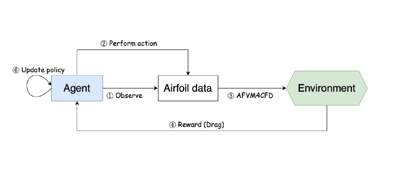
Figure 3: Reinforcement Learning Framework.

At each time step $t$, the standard MDP process is defined by a 4-tuple $(S_{t},A_{t},P_{t},R_{t})$ [54] which contains the interaction between agent and environment, where $t=0,1,2,\cdots.$ Here $S_{t}$ represents the state, which consists of the mesh points that depict the geometry of the airfoil at time step $t$. $A_{t}$ stands for the action performed on $S_{t}$. The action $A_{t}$ consists of three parameters $[x_{target},y_{Uchange},y_{Lchange}]$. For a given $x$ coordinate $x_{target}$, there exists a pair of points on both curves whose values on $y$ direction are $y_{upper}$ and $y_{lower}$. Then the $y$ coordinates will be updated with parameters $y_{Uchange}$ and $y_{Lchange}$ on both curves respectively. However, the values will not only be acted with respect to $x_{target}$. This behavior introduces a sharp deformation, which will bring singularity to the geometry and may even cause a mesh tangling phenomenon. To perform a more smooth and natural action on the airfoil, we utilize a smooth technique as shown in Figure 4. For a specific $x_{target}$, the update value $y_{Uchange}$ will not be acted on the point directly. The delta function is defined as

$$SA(x)=e^{-\frac{(x-x_{target})^{2}}{2\delta^{2}}}$$ (15)

will be set as a coefficient that can smoothen the deformation process. $\delta$ is set to $0.2$ to $0.8$ in this model. Then the $y$ coordinate of the upper curve will be updated with

$$y^{\prime}=y+y_{Uchange}SA(x).$$ (16)

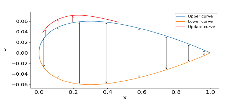
Figure 4: Update curve with a smooth action.

As explained above, a specific airfoil shape is a single point in a high-dimensional space. If the update value is just an entry in the vector formulated by shape, the difference between the update vector and the original vector is weeny. As a result, the agent may not notice such discrepancy and is not capable of performing tactful action. The smoothing process not only improves the efficiency during the optimization but also assists the action learning process by amplifying the difference between tensors.

After the deformation, the algorithm of curve fitting will generate the Bézier curves, which will be explained later. The update points represent the new state of the airfoil, $S_{t+1}$. At each time step, there are various actions that the agent can take. $p(S_{t+1}|S_{t})$ is denoted as the transition probability for the state $S_{t}$ change to $S_{t+1}$ with action $A_{t}$. The agent will evaluate the potential reward from different actions. The action that the agent takes at state $S_{t}$ is $A_{t}$, which is generated from the policy $\pi_{t}:S_{t}\rightarrow A_{t}$. The agent will evaluate the reward $R_{t+1}(S_{t},A_{t},S_{t+1})$ from the environment and try to maximize the cumulative reward from a potential trajectory $\tau$, which is given by

$$\tau=(S_{0},A_{0},S_{1},A_{1},\cdots,S_{t},A_{t},\cdots).$$ (17)

In this trajectory, the cumulative reward at time step $t$ is defined as

$$G_{t}(\tau)=\sum_{i=0}^{T}\gamma^{i}R_{t+i+1}.$$ (18)

Then the agent shall be trained to maximize the reward so that the deformation can fulfill the optimization target. Various deep learning algorithms have been constructed in the past decades like the Deep Q Networks(DQN), Double Deep Q Networks (DDQN)[55], Proximal Policy Optimization[56] (PPO) and Twin Delayed DDPG(Deep deterministic policy gradient)[57]. Among the algorithms, the Twin Delayed DDPG algorithm is constructed in this work for its efficiency in continuous space and is suitable for the current framework. In the following subsection, we start with the original DDPG algorithm to understand the shape optimization process with reinforcement learning. Then the Twin Delayed DDPG algorithm is a melioration based on this framework.

4.2 Deep deterministic policy gradient for training

We start with the basic DDPG algorithm to understand the optimization process of the airfoil shape optimal design. The DDPG framework consists of two primary components: the actor and the critic, each with its distinct role in learning the optimal policy. The actor, parameterized by $\theta^{a}$, is responsible for determining the best possible action $A_{t}$ given the current state $S_{t}$ at time step $t$ with the current policy, i.e., $A_{t}=\pi_{\theta^{a}}(S_{t})$. This direct policy optimization allows the DDPG algorithm to efficiently explore the continuous action space and identify optimal actions.

Since the actor may generate potential actions that form a state-action sequence, i.e., $\tau_{\theta^{a}}\sim\pi_{\theta^{a}}$. The cumulative reward at time step $t$ is not explicitly calculated because the reward should be obtained from the CFD solver, which is generally time-consuming. The critic, on the other hand, parameterized by $\theta^{c}$ evaluates the quality of the actions proposed by the actor within the current policy. Hence, $\tilde{R}_{t+1}(S_{t},A_{t}|\theta^{c})$ is the reward calculated by the critic with a neural network. For a specific long term state evolution $\tau$,

$$\tilde{G}_{t}(\tau_{\theta^{a}}|\theta^{c})=\tilde{R}_{t+1}(S_{t},A_{t}|\theta^{c})+\sum_{i=1}^{T}\gamma^{i}\tilde{R}_{t+i+1}\Big{(}(S_{t+i}|\theta^{a}),(A_{t+i}|\theta^{a})|\theta^{c}\Big{)}.$$ (19)

is defined as calculating the expected cumulative reward. The Q-value, which is represented as

$$Q(S_{t}|\theta^{a},\theta^{c})=\mathbb{E}_{\tau_{\theta^{a}}\sim\pi_{\theta^{a}}}\Big{(}\tilde{G}_{t}(\tau_{\theta^{a}}|\theta^{c})\Big{)}$$ (20)

is adopted to assess the performance of the actor with current parameters $\theta^{a}$. The critic guides the actor towards actions that maximize the long-term reward. The feedback of critic is essential for updating the parameters of actor and refining the policy.

During training, a replay buffer is utilized to store and randomly sample previous transition tuples $(S_{t},A_{t},S_{t+1},R_{t+1})$ facilitating the learning of uncorrelated and diversified experiences. This experience replay mechanism significantly stabilizes and enhances the training process by preventing the correlation of consecutive experiences and reducing the variance of the updates.

In the training process, the critic is updated by minimizing the mean squared error between a batch of current Q-values and the batch of target Q-values, which are calculated based on the next state and the next action proposed by the actor. The actor is then updated by performing gradient ascent on the expected Q-values output by the critic, thus steering the actor towards actions that yield higher rewards.

Through the interaction between the actor and the critic, the DDPG framework effectively navigates the continuous action space with the experience in the replay buffer. As a result, the agent is able to learn sophisticated policies and perform expected actions on the airfoil, thereby optimizing its performance in complex environments. A brief algorithm of this DDPG training process is organized as follows:

Data: Wing shape data, DDPG agent with actor and critic networks, ReplayBuffer

Result: Trained DDPG agent

1 for each episode in max_episodes do

2       Reset the environment and get the initial state;

3       while the episode is not done do

4             The agent selects and executes an action;

5             Observe the new state and the reward;

6             Save the tuple (state, action, reward, next_state) to the ReplayBuffer;

7             if ReplayBuffer has enough experiences then

8                   Sample a batch of experiences from ReplayBuffer;

9                   Use the batch of experiences to train the actor and critic networks;

10                  

11             end if

12            Update the state;

13            

14       end while

15      

16 end for

Algorithm 2 Deep Deterministic Policy Gradient (DDPG)

4.3 Mesh deformation for unstructured mesh

The mesh deformation during the shape optimization is a complicated process. It is important to ensure the quality of the mesh is capable of the calculation of target functional. The process of mesh deformation, modification, and calculation process can be organized as shown in Figure 5.

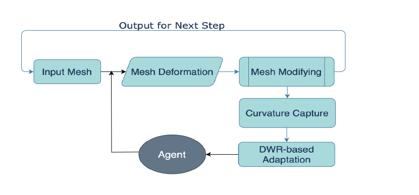
Figure 5: Mesh deformation, modification, and calculation process during the reinforcement learning

To conduct the deformation of the airfoil, we need to adopt the parameterized curve for depicting the geometry at first. In this study, we applied the Bézier curves representation for the parameterization. The airfoil consists of an upper curve and a lower curve. For a given $x$ coordinate, there exists a pair of $y$ coordinates on the two parts. The representation for such two parts can ensure the $y$ coordinate of the upper half is always larger than that of the lower part so that the two curves will not intersect and prevent the mesh from tangling.

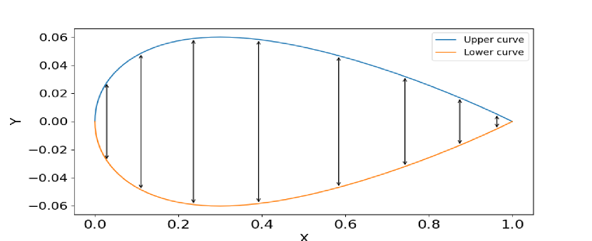
Figure 6: Airfoil consists of two parts.

With the Bézier least square fitting, a series of control points can be calculated with the mesh points along the airfoil where the number of control points can be set manually. Then the Bézier curves can be generated by the Bernstein polynomials, i.e.,

$$B(t)=\sum_{i=0}^{n}\binom{n}{i}(1-t)^{n-i}t^{i}CP_{i}.$$ (21)

Here $B(t)$ represents the Bézier curve itself, which is a function of the parameter $t$. $t$ ranges from $0$ to $1$ which essentially interpolates between the control points $CP_{i}$. Then we set the airfoil with the defined curve in a circle with a large enough radius. With such a technique, we defined the computational domain on an unstructured mesh, and the mesh around the airfoil is shown in Figure 1. The airfoil is depicted with a determinate number of mesh points. The order of these mesh points is arranged in an anticlockwise direction from the tail endpoint and forms a closed cycle.

When the agent of reinforcement learning tries to modify the shape of airfoils, it will change all the mesh points. Equivalently, the control points will be updated and result in varied Bézier curves. From the updated expression of Bézier curves, we can calculate the mesh points along the airfoils in an anticlockwise direction. Afterward, we build a map structure so that the mesh file can find the corresponding mesh points on the airfoils and update their coordinates. As shown in the left part of Figure 7, the geometry received the action from the agent and the shape gets updated.

Figure 7: Left: mesh around the deformed shape before the modifying; Right: mesh around the deformed shape after the modifying;

However, it is shown in the left part of Figure 7 that the quality of mesh gets influenced since the movement of boundary mesh points may lead to a sharp acute angle for the triangles near the upper curve and a large obtuse angle for the triangles near the lower half. While the optimization lasts for a long period, the phenomenon of mesh tangling will get more serious with iteration steps. Hence we shall modify the mesh so that it is capable of multi-step mesh deformation. In numerical simulation, it is never suggested to bring sharp transformation to the numerical scheme like geometry and solution update. Hence the movement of points is restricted to a specific scale. Then the deformed mesh should be modified for further calculation. Since the most closely affected elements are those on the boundary part, such area should be processed specially. For those boundary elements that have two points on the airfoil, the third point is relocated so that this element will be a regular triangle. Then we adopted the Laplacian smoothing technique to amend the quality of the mesh. The fundamental operation in Laplacian smoothing involves updating the position of a node to be the average of the positions of its neighboring nodes. Mathematically, this can be expressed as

$$\mathbf{x}_{i}^{{}^{\prime}}=\frac{1}{m}\sum_{j=1}^{m}\mathbf{x}_{j},$$ (22)

where $\mathbf{x}_{i}$ is the coordinate vector of the $i$-th point and $\mathbf{x}_{i}^{{}^{\prime}}$ is the update value. $\mathbf{x}_{j}$ with index from $1$ to $m$ are neighboring nodes of corresponding $i$-th point. With such a modification process, the quality of the mesh is enhanced. As shown in the right part of Figure 7, the elements around the airfoil are recovered so that sharp acute angle and large obtuse angle can be prevented.

To implement such mesh recovery within our algorithm, only adopting smoothing techniques is not sufficient as it cannot preserve the desired properties of boundary-sensitive points. Aiming to maintain efficiency throughout the iterative process, remeshing is not considered since it is time-consuming, especially when generalized to three-dimensional cases. Even though the post-smoothing mesh possesses improved structural integrity of the triangular elements, it should not be far away from the pre-processed state. To this end, we utilize the map data structure inherent in C++ for its capability to manage modifications without drastically altering point positions or changing the number of vertices within the mesh.

In our approach, vertices that are not on the boundary but belong to boundary triangles are assigned with level 1. Subsequently, vertices without a level, belonging to triangles that include level 1 vertices, are marked as level 2. We then recalculate the triangles containing level 1 and level 2 vertices so that the new triangles can approximate an equilateral triangle as possible. This recalculated position is mapped against the initial position, facilitating updates to the mesh data file through these mappings. Thus, without a remeshing process, we achieve a recovery of mesh properties. It helps the mesh remain similar to its original state while significantly enhancing the quality of the triangular elements. This method allows for an effective improvement in mesh quality, crucial for the accuracy of subsequent simulations and analyses.

It is worth noting that when the agent tries to modify the geometry, the curvature of the airfoil changes rapidly. The deformation conducted with a scale comparable to the mesh size can be handled with the method mentioned above. However, when the scale is smaller than the mesh size, the given mesh points can not detect such curvature variation within the segment. Then, it will add noise to both the primal and dual equations, and return an imprecise reward back to the agent. As a result, it will bring more complexities and increase training difficulties. For this reason, we shall use triangles with a smaller scale.

Figure 8: Mesh around the tail before curvature capture; Mesh around the tail after curvature capture.

To calculate the curvature for each boundary curve, we shall find the parameters correspond with the endpoints, $t_{1}=B^{-1}(\mathbf{x}_{1})$ and $t_{2}=B^{-1}(\mathbf{x}_{2})$. Then we generate sample points that are dense enough within such segment, $sp_{0},sp_{1},\dots,sp_{L+1}$. For three consecutive sample points $sp_{i-1},sp_{i},sp_{i+1}$, we use $\theta_{i}$ to denote the angles between $\overrightarrow{sp_{i-1}sp_{i}}$ and $\overrightarrow{sp_{i}sp_{i+1}}$, then $\kappa_{i}={\theta_{i}}/{\|\overrightarrow{sp_{i}sp_{i+1}}\|}$ is used to denote the discrete curvature values. $\sum_{i=0}^{L}\kappa_{i}$ is used to denote the curvature change within the segment. It is shown in the left part of Figure 8, that if the curvature change scale is smaller than the mesh size like the elements near the tail, the mesh can not detect such variation. However, when we use elements with smaller sizes, it can capture the curvature change within the segment. After running this algorithm for several times, the mesh can depict a more elaborate airfoil shape.

4.4 Curve smoothing

The reinforcement learning process in this framework necessitates a delicate balance between the granularity of the sample points and the computational feasibility. High-dimensional state representations, while offering detailed control over the geometry, exacerbate the curse of dimensionality. This not only makes the optimization landscape more complex and harder to navigate but also strains the underlying PDE solvers. For machine learning-based solvers, deviations from the trained geometries can result in diminished accuracy, adversely affecting the fidelity of the objective functional evaluations. This necessitates the integration of traditional numerical methods capable of handling a wider variety of shapes with robustness, ensuring high precision in objective functional computation irrespective of the geometric configuration.

Furthermore, excessive sample points can introduce local singularities and discontinuities in the geometry, making it highly non-smooth such as shown in the left part of Figure 9. While actual engineering solutions rarely embody such erratic geometric characteristics, their presence during the learning process can significantly affect the optimization. Non-smooth geometries not only challenge the solver’s capacity to provide accurate solutions but also obscure the learning signal, making it difficult for the agent to discern productive learning directions. Such geometric irregularities could mislead the agent, leading to suboptimal policies that fail to converge to the desired outcome.

Figure 9: Left: mesh around the shape without curve smoothing; Right: mesh around the shape with the curve smoothing;

A refined approach entails leveraging dimensionality reduction and feature engineering to extract and condense essential geometric features into a more succinct and computationally efficient representation. While directly reducing the dimensionality of sample points may compromise their utility for precise geometric manipulation, alternative strategies can offer a balance between detail and manageability. The utilization of the Bézier curve fitting adopted above stands out as a proficient technique for reducing dimensionality while capturing critical curve characteristics. This method effectively summarizes vital information, facilitating a streamlined representation of curves. However, the challenges still persist, particularly regarding the smoothness of the curves. Merely lowering the order of Bézier curves can inadvertently eliminate valuable local details. To circumvent these issues, incorporating smoothing techniques during the Bézier curve generation process emerges as a potent solution. Integrating regularization directly into the curve fitting algorithm ensures the smoothness of the curves, preserving the integrity of local geometric features without sacrificing the overall quality of the representation.

The Bézier curve fitting adopted above is :

$$\begin{array}[]{cc}&\text{Find}\qquad\{CP_{i}\}_{i=0}^{n},\\ &\min\qquad\sum_{j=0}^{L+1}|\!|B(t_{j})-sp_{j}|\!|^{2}\end{array},$$ (23)

where $t_{j}$ is the parameters corresponding to the sample points $sp_{j}$. With the regularization term added to the system, the equation becomes:

$$\begin{array}[]{cc}&\text{Find}\qquad\{CP_{i}\}_{i=0}^{n},\\ &\min\qquad\sum_{j=0}^{L+1}|\!|B(t_{j})-sp_{j}|\!|^{2}+\lambda_{s}*\sum_{i=1}^{n-1}|\!|CP_{i-1}-2*CP_{i}+CP_{i+1}|\!|^{2}\end{array},$$ (24)

where $\lambda_{s}$ stands for the smoothing coefficient. The impact of this regularization term is to make the control points distributed equidistantly. As a result, the potential issues of the non-smooth curve can be mitigated effectively. As shown in the right part of Figure 9, the deformed curve preserves a satisfactory geometry while having a detailed control of the airfoil.

5 Design of Twin Delayed DDPG

In the previous section, we have established a simple framework that can manipulate the deformation of the airfoil shape. However, training an agent to achieve the goal of interacting with the environment in such a complicated process is not straightforward. Firstly, the dimension of the state is defined by hundreds of points. During the initial stage, the difference between the tensor representation of different airfoils is tiny. Then the agent may not detect the features of different airfoils. Secondly, the inherent relation between the state and action with corresponding action parameters is intricate. Since the authentic value of reward needs the calculation with a CFD solver, the critic neural network is adopted to approximate such a process. The neural network of reinforcement learning is usually constructed with a light structure since the sampling is expensive, and the result shall be obtained quickly for a long-term iteration. Conversely, a simple neural network is not accurate enough to capture the relation between these variables. Meanwhile, a complicated neural network suffers a lot from the gradient disappear problem, leading to the training invalid. Thirdly, during the training process, the agent may fail to learn the optimization method if it can not obtain a positive reward. How to guide this agent to take appropriate actions on the airfoil is crucial for the policy update. Last but not least, the DDPG framework suffers a lot from the overestimate. With the development of an algorithm in reinforcement learning, the Twin Delayed DDPG framework remits such influence efficiently and enhances the training performance. In this section, we focus on these issues and elaborate on the details of the Twin Delayed DDPG framework for the design of airfoil.

5.1 Actor and critic

The actor is developed to choose the potential action based on the input state such that the obtained reward is maximal. While the state is the tensor representation of the corresponding airfoil shape, the actor should capture the main feature and distinguish different shapes. Aiming at having a precise control of the airfoil, the geometry is constructed with hundreds of points pair. However, the agent may fail to learn valuable actions based on different states when this tensor representation is conducted within a high-dimensional space. A new state conducted by a specific action only takes a small change of target location. Such difference is easy to overlook within a hundred-dimensional tensor. The smooth action process explained in the previous section can remit such influence but the essential difficulties have not been solved. Trying to conduct the deformation within a lower dimensional tensor space, we considered adopting the variational autoencoder(VAE) module at first.

• Variational autoencoder

  The module contained a neural network that is designed to capture complex relationships between different airfoils, which is crucial for accurately modeling the state space in the wing design problem. The VAE will help in generating new, valid states that conform to the physical constraints of the wing design, aiding in exploring the state space more effectively. The encoder part of VAE maps the variable to a distribution in the latent space, rather than a single point. This is typically a Gaussian distribution characterized by vectors of means $\mu_{vae}$ and log-variances $\sigma_{vae}$. It is capable of learning the generative process for complex data. In this context, by learning how existing wing shapes are generated, a VAE can help in determining the actions to take for optimizing new designs.

  To guarantee the latent layer captured the key feature of airfoil data $\mathcal{X}$, the decoder part will reconstruct the latent representation to $\widetilde{\mathcal{X}}$. The standard loss function for the VAE is a combination of two distinct terms: the reconstruction loss and the Kullback-Leibler (KL) divergence[58]. The reconstruction loss measures the difference between the original input data $\mathcal{X}$ and the reconstructed data $\widetilde{\mathcal{X}}$ produced by the decoder of the VAE. It ensures that the VAE is capable of accurately reconstructing inputs, which means that the latent space is capturing the necessary information about the data distribution.

Layer Type	Layer Name	Operation	Output Channels	Activation
Input	input	-	15 * 2 * 2	-
Actor
nn.LayerNorm	norm1	Layer Normalization	256	-
ResidualBlock	res_block1	Residual Block	256	-
nn.Linear	fc	Linear	512	SELU
nn.LayerNorm	norm2	Layer Normalization	512	-
nn.Linear	layer_action_param	Linear	128	SELU
Postprocessing
nn.Linear	action_probability	Linear	3	softmax
nn.Linear	action_param	Linear	5	softsign

Table 1: Actor Network Architecture

The variational autoencoder meets the requirement of dimensionality reduction efficiently. However, it brings extra problems to the construction of the learning process. Firstly, it is not easy to take the balance of the reconstruction error and original loss function. Secondly, deeper neural networks aggravate the risk of the gradient disappearance problem. Thirdly, the sampling process is expensive in this reinforcement learning task. The VAE module can not perform well with limited data and gets trapped into overfitting issues. Additionally, failures of this model may be attributed to the reasons as follows. If we collect the $266$-dimensional tensors representing the airfoil, each tensor can be treated as a point within this high-dimensional space. Specifically, points that conform to closed-curve airfoil geometries form a submanifold within this space. This submanifold is non-convex since states between distinct airfoil shapes may include mesh tangling form. The probability that these points are collected is $0$ since we avoid such circumstances with the methods mentioned above. The challenge of dimensionality reduction in this context is underscored by the difficulty in preserving geometric and topological properties during the mapping to a lower-dimensional space, a process complicated by the non-convex nature of the submanifold. As a result, the VAE model faces significant hurdles in accurately representing such complex, non-convex geometries without incurring substantial reconstruction errors. The optimal transportation method proposed in [59] aims at finding a measure-preserving map that minimizes the total transport cost. However, it may not be practical for our current framework to conduct analysis with the collected data in a large magnitude.

Then we tried a different method, using Bézier curves representation for the dimensionality reduction. The Bézier curves take the most important information for specific curves. Besides, the difference between different control points originating from corresponding states is amplified with the least square process. It helps the agent to distinguish different states. Meanwhile, as an independent process, it avoids the gradient calculation within a neural network.

Layer Type	Layer Name	Operation	Output Channels	Activation
Input	input	-	66 * 2 * 4	-
Attention Module
nn.linear	state2hidden	Linear	64	SELU
nn.linear	action2hidden	Linear	64	SELU
nn.linear	param2hidden	Linear	64	SELU
nn.MultiheadAttention	self_attn	Self-Attention	64	-
nn.MultiheadAttention	cross_attn	Cross-Attention	64	-
Critic processing
ResidualBlock	res_blockCritic1	Residual Block	512	SELU
ResidualBlock	res_blockCritic2	Residual Block	128	SELU
nn.Linear	fusion_fc2	Linear	8	SELU
nn.Linear	q_value_fc	Linear	1	-

Table 2: Critic Network Architecture

The dimension is reduced efficiently with the Bézier curve representation. Then the information should be processed through the neural network constructed as Table 1 to obtain the action that maximizes the reward from the current state. It should be noted that the output includes action probability for different types of action and corresponding parameters that action possesses. The action that is chosen to be performed originates from the $softmax$ layer while the corresponding parameters are based on the restriction of shape design. For fear of mesh tangling, an activation function needs to be designed that maps the parameters to reasonable intervals. However, the traditional activation functions like $tanh$ and $sigmoid$ suffer a lot from the gradient disappear phenomenon. Then the $softsign$ type activation function is adopted. Furthermore, the residual connection module is also integrated to guarantee the gradient can be propagated normally within the neural network.

The critic neural network is designed to evaluate the potential feedback for various actions acted on different states based on the experience accumulated in the replay buffer. The reward mechanism is complicated since the data originate from a CFD solver, not even to mention the shape deformation. In order to approximate such a process, the interaction between the shape, actions and corresponding parameters should be modeled efficiently. We considered adopting the self-attention and cross-attention mechanism together to investigate the inherent relation. The self-attention mechanism can detect those features which take a significant influence on the target functional. Meanwhile, the cross-attention mechanism is adopted to approximate the shape deformation process. In other words, it tries to understand how the action with corresponding parameters influenced the shape deformation. The state, action, and action parameters are mapped to the hidden layer with the same dimension to ensure the cross-attention layer can be modeled.

The loss function is an important component of the learning framework which decides the update direction of parameters in neural networks. For different modules in reinforcement learning, the loss function is defined according to the features. In order to choose the action that maximizes the reward based on specific states, the agent should evaluate the potential feedback correctly at first. It indicates that the critical neural network should be updated more frequently than the actor neural network. The long-term reward loss is defined as

$$Critic\_loss={R}_{t+1}(S_{t},A_{t}|\theta^{c})+\gamma*Q(S_{t+1}|\theta^{a},\theta^{c})-Q(S_{t}|\theta^{a},\theta^{c})$$ (25)

is adopted to minimize the error of long-term reward based on the real reward of the environment. The selection of the loss function for the actor network is designed to effectively guide the policy towards actions that maximize expected rewards. This is achieved through a gradient ascent approach on the expected return. The maximal reward loss is typically defined as the negative of the Q-value estimated by the critic network for the current state and the action proposed by the actor network, i.e.,

$$Actor\_loss=-Q(S_{t}|\theta^{a},\theta^{c}).$$ (26)

With the actor and critic neural networks, the agent interacts with the environment and tries to accumulate experience to perform appropriate actions based on different states. The learning performance is highly related to data originating from the interaction process. In order to enhance efficiency, the exploration should incorporate sufficient states. Otherwise, the exploitation may get trapped into overfitting issues. While the shape optimal design of airfoil is a complicated process and not easy to be trained for solving specific target functional, we ameliorate the exploration and exploitation process as follows.

5.2 Exploration and exploitation

Exploration and exploitation are fundamental components of the interaction process. The agent tries different actions to gain information about the environment during the exploration process. Extensive exploration is crucial since the agent needs to try different actions to gain more information about the environment within an unfamiliar task. It helps avoid local optima and enables the agent to find more effective strategies. Then the agent uses its existing knowledge or experience to make decisions that maximize immediate rewards during the exploitation period. Balancing exploration and exploitation is vital in reinforcement learning. Excessive exploration can prevent the agent from fully utilizing known effective strategies. On the other hand, too much exploitation might cause missing out on better strategic options. In this framework, we adopt the $\epsilon$-greedy strategy. This is a popular technique that chooses an action at random with probability $\epsilon$ and selects the action that is predicted to have the highest reward based on its current knowledge with probability $1-\epsilon$. Besides, in our framework, we integrate Ornstein-Uhlenbeck (OU) noise as a complementary tool to the $\epsilon$-greedy strategy, specifically targeting the exploration aspect of reinforcement learning in continuous action spaces. While the $\epsilon$-greedy strategy efficiently balances exploration and exploitation by randomly selecting actions with a probability $\epsilon$, OU noise adds an additional layer of sophistication to the exploration process.

Even though the optimization mechanism can be well implemented with the exploration and exploitation process, the learning effect is not ideal usually. The difficulties originate from the complex mechanisms involved in airfoil design. Firstly, it is not easy to identify the correct reward direction in random exploration. Excessive penalization can lead the neural network parameters into an unfavorable bottleneck, where the agent opts for minimal action to avoid penalties, eventually leading to a suboptimal local optimum. Secondly, airfoil design inherently demands a geometry with a certain level of smoothness. If the shape changes drastically in a single step, even a correct design trend may result in unfavorable reward feedback due to geometric roughness. This also indicates that the shape optimal design needs to be implemented within an elaborate parameter representation environment. Thirdly, the training batch size is small during the initial stage since the available data is limited. A smaller batch size can lead to more noise in the gradient estimates, which can inadvertently aid exploration by preventing the model from quickly converging to a local optimum. However, this noise can also result in less stable learning, as the updates might oscillate or diverge.

To address the above issues, we introduced several improvement strategies as follows, i). if a certain action results in a penalty, the agent attempts to explore the opposite direction starting from the pre-deformation geometry. Both exploration results and parameters are stored in the replay buffer, and the action leading to a better outcome is chosen for the next step. This mechanism significantly reduces aimless, detrimental exploration in airfoil design, preventing the model from extensively exploring in unproductive directions. This is also inspired by the idea of a twin network to prevent oscillation during the simulation and it turned out to be very effective for reinforcement learning. Similarly, if the current action brings a perfect reward, the agent will be encouraged to take a similar action with a tiny noise. As the environment is not straightforward to obtain positive meaningful rewards, such a mechanism can help the agent to accumulate useful experience quickly. ii). the single step movement of the sample points is constrained, so that there may not occur singular geometry. Besides, an early stop mechanism is constructed when the accumulated reward decreases to the minimum threshold. This can be explained as the agent failing for the current design process when the geometry gets trapped into a very terrible shape and may not recover easily. Then the environment should be reset for the next turn. iii). the training process is separated into different periods. A small batch size is adopted for the initial stage. When the replay buffer accumulates enough data, a larger batch size number will be updated. Besides, the data are stored in the replay buffer with a 4-tuple form transition $(state,action,action\_parameters,next\_state)$. Every time the gradient should be calculated from the 4-tuple with a number of batch sizes. The components include three parts, the recent transitions, the transitions with the best reward and randomly chosen transitions from the whole memory. The recent transitions represent the behavior under the current parameters of neural networks while the best transitions can help the agent to repeat the beneficial actions and the random transitions can make the gradient calculation more stable. With such efficient exploration and exploitation mechanisms, we step further to fulfill the reinforcement learning framework.

5.3 Reward function

In the context of shape optimal design, the reward function must match the optimization objective. For instance, consider the objective of generating a shape with the minimum drag, denoted as $D(\{sp_{i}\}_{i=0}^{L+1})$, where $\{sp_{i}\}_{i=0}^{L+1}$ represents the sample points of the airfoil with minimal drag. This relationship is described by the following equation:

$$\begin{array}[]{cc}&D(\{sp^{*}_{i}\}_{i=0}^{L+1})\leq D(\{sp_{i}\}_{i=0}^{L+1})\qquad\forall sp_{i}\in\mathbb{R}^{2}\\ &\{sp^{*}_{i}\}_{i=0}^{L+1}\equiv\{sp_{i}\}_{i=0}^{L+1}\quad\text{if\leavevmode\nobreak\ }D(\{sp_{i}\}_{i=0}^{L+1})\leq D(\{sp^{*}_{i}\}_{i=0}^{L+1})\end{array}$$ (27)

To simplify, we denote the drag at time step $t$ as $D_{t}$. The reward function at time step $t$ is then defined as:

$$R_{t}=D_{t-1}-D_{t}.$$ (28)

Intuitively, the reinforcement learning process aims to maximize the cumulative reward $\sum_{t=1}^{T}R_{t}$. A pertinent question arises as to whether this optimization goal is equivalent to the original objective. If we define $\{sp^{**}_{i}\}_{i=0}^{L+1}$ as the sample points of the airfoil yielding the maximal reward, then:

$$D_{0}+(-D(\{sp^{**}_{i}\}_{i=0}^{L+1}))\geq D_{0}+(-D(\{sp_{i}\}_{i=0}^{L+1}))\qquad\forall sp_{i}\in\mathbb{R}^{2}.$$ (29)

More specifically,

$$D_{0}+(-D(\{sp^{**}_{i}\}_{i=0}^{L+1}))\geq D_{0}+(-D(\{sp^{*}_{i}\}_{i=0}^{L+1}))$$ (30)

The equation above can be converted to:

$$D(\{sp^{**}_{i}\}_{i=0}^{L+1})\leq D(\{sp^{*}_{i}\}_{i=0}^{L+1}).$$ (31)

By definition, $\{sp^{**}_{i}\}_{i=0}^{L+1}$ is equivalent to $\{sp^{*}_{i}\}_{i=0}^{L+1}$, demonstrating the equivalence of the reinforcement optimization objective to the primary task. A similar proof, such as maximizing the lift-drag ratio, can also be derived in this manner.

In our shape optimization tasks, the optimization process incorporates additional components beyond the straightforward maximization of cumulative rewards. As mentioned in the previous section, the discount factor $\gamma$ plays a pivotal role in calculating the cumulative reward. The discount factor ensures that the optimization process remains focused on achievable improvements, preventing the pursuit of impractically distant objectives.

To further refine the optimization strategy, regularization terms can be added to the reward function. These terms are designed to encourage exploration, a critical aspect of overcoming local optima and discovering globally optimal solutions. By incorporating exploration-driven regularization, the reward function can be represented as:

$$R_{t}=(D_{t-1}-D_{t})+\lambda^{\epsilon}_{E}\cdot(D_{0}-D_{t}),$$ (32)

where $\lambda^{\epsilon}_{E}$ is a weighting coefficient that balances the original objective with the exploration incentive. When the current shape yields an improvement in the objective function value, the agent gets reward. Conversely, a penalty is incurred for generating a geometry that does not meet the expected criteria. The parameter $\lambda^{\epsilon}_{E}$ shall be decreased with the update of noise. Thus the reward function will encourage exploration for the initial period while it converges to the equation (28) with the iteration get processed. Theoretically, the result shall be equivalent to the primal objective. These mechanisms ensure a more robust and effective search for the optimal airfoil shape, facilitating the discovery of innovative designs that minimize drag while navigating the complex landscape of possible configurations.

5.4 Twin delayed DDPG

With the introduced modules above, we are going to develop our framework to a more robust version, Twin Delayed Deep Deterministic Policy Gradient, which is an algorithm that builds upon the Deep Deterministic Policy Gradient framework. It introduces several key improvements that enhance stability and performance in reinforcement learning tasks. One of the primary advantages of Twin delayed DDPG is its twin-critic network architecture. This design involves using two separate critic networks to estimate the Q-values, and the smaller of the two Q-value estimates is used for the policy update. This approach effectively reduces the overestimation bias often seen in DDPG, leading to more stable and reliable learning.

Additionally, Twin delayed DDPG introduces policy update delays, where the policy network is updated less frequently than the critic networks. This delay helps mitigate the risk of the policy network exploiting inaccuracies in the Q-value estimates, further enhancing the stability of the learning process. Twin delayed DDPG also applies target policy smoothing, adding noise to the target action, which smoothens the value estimate and prevents the policy from exploiting Q-function errors in sharp transitions.

With this more stable reinforcement learning framework, we constructed the algorithm as Algorithm 3.

Data: Initial wing shape data, actor parameters $\theta^{a}$, critic parameters $\theta^{c_{1}}$ and Twin critic parameters $\theta^{c_{2}}$, target networks $\theta^{a}_{target}$, $\theta_{target}^{c_{1}}$ and $\theta_{target}^{c_{1}}$, ReplayBuffer

Result: Trained Twin Delayed DDPG agent

1 Set the target parameters $\theta^{a}_{target}\leftarrow\theta^{a},\theta^{c_{1}}_{target}\leftarrow\theta^{c_{1}},\theta^{c_{2}}_{target}\leftarrow\theta^{c_{2}}$

2for each episode in max_episodes do

3       if Exploration or reach the minimum threshold then

4            Reset the environment and get the initial state

5       end if

6      for step in episode do

7             if Exploration then

8                   The agent produces a random action for execution

9             end if

10            else

11                  The agent selects an action based on $\theta^{a}_{target}$

12                  Noises are added to the action and corresponding parameters

13                  The agent executes the action based on the current state

14                  Update the cache state

15             end if

16            Observe the new state and calculate the reward based on AFVM4CFD;

17             if reward $<min\_reward$ then

18                   Reload the cache state

19                  Execute the opposite action with corresponding parameters

20             end if

21            

22            Save the tuple (state, action, reward, next_state) to the ReplayBuffer;

23             if ReplayBuffer has enough experiences then

24                   Sample experiences (Recent, Best, Random) from ReplayBuffer;

25                   Compute the target actions based on $\theta^{a}_{target}$;

26                   Compute the target Q-value $\min(Q_{\theta_{target}^{c_{1}}},Q_{\theta_{target}^{c_{2}}})$;

27                   Update the critic networks $\theta^{c_{1}}$, $\theta^{c_{2}}$ ;

28                   Soft update critic networks $\theta_{target}^{c_{i}}\leftarrow\theta_{target}^{c_{i}}*\tau+(1-\tau)*\theta^{c_{i}}$ for $i=1,2$

29                  if $step\equiv 0\pmod{delay\_step}$  then

30                         Update the actor network $\theta^{a}$ ;

31                         Soft update actor networks $\theta_{target}^{a}\leftarrow\theta_{target}^{a}*\tau+(1-\tau)*\theta^{a}$

32                   end if

33                  

34             end if

35            Update the state;

36            

37       end for

38      

39 end for

Algorithm 3 Twin Delayed Deep Deterministic Policy Gradient

6 Numerical Result

6.1 Minimize drag optimization

The initial example delves into minimizing drag calculations, a process whose precision is bolstered by the DWR-based mesh adaptation method. The study utilizes a NACA0012 airfoil, positioned within a circular domain with a radius of $35$, under a boundary condition of mirror reflection. The operational conditions are set with a Mach number of $0.85$ and an attack angle of $0^{\circ}$.

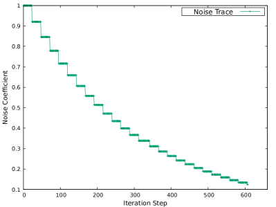
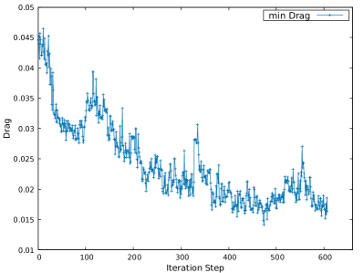
Figure 10: Left: the record curve of noise coefficient. Right: the record curve of drag during the optimization process.

To ensure the integrity of the airfoil’s structure during training, a constraint is imposed, mandating a minimum thickness of 0.1 for sections where $x<0.1$ and $x>0.7$. Should a potential action result in an airfoil design adhering to this thickness constraint, it is deemed physically infeasible, consequently not executed, and results in the issuance of a negative reward.

As delineated in Algorithm 3, the agent embarks on accumulating experience through random actions performed four times, each starting from the baseline configuration and geometry across $64$ time steps. The initial recorded drag value stands at $0.0452106$.

Figure 11: Left: the airfoil generated from the 15th episode. Right: the result of the optimized airfoil.

Training commences with a moderate batch size of $256$, spanning a total of $75$ epochs, with each epoch comprising 8 time steps. The noise coefficient undergoes adjustment every three epochs, following an exponential decline. As illustrated in Figure 10, the drag value exhibits a decrement trend as iterations advance. Even though the record curve is not smooth while the drag value gets increased at some moment, it still evolved towards the optimization objective. The non-smooth phenomenon originates from the fact of noise. Even if the potential action from the actor neural network generates an effective action with corresponding parameters, the noise may distract the agent from the potential actions. However, such a noise module is indispensable to help the agent explore the possibility of different states.

Throughout the optimization process, the agent probes various airfoil shapes. For instance, Figure 11 showcases a configuration from the $15^{th}$ epoch, sporting a drag value of $0.031537$. The drag value’s trajectory halts around $0.02$, constrained by the minimum thickness stipulation. Encounters with this boundary condition trigger a negative reward, steering exploration toward alternate states. Notably, as the exploration progresses, particularly in the concluding epoch, the airfoil’s tail approaches the thickness restriction, a direct consequence of rewards associated with thickness reduction.

The reduction in drag can be elucidated by examining the Mach isolines. Initially, the NACA 0012 airfoil exhibited strong shock waves on both sides of the wing, typically associated with significant pressure jumps near these shocks, contributing to a large value of drag. However, the optimized airfoil shape through our process demonstrates a significant transformation in shock wave structure. The shock wave on the upper part of the airfoil has weakened and shifted its position, while the shock wave on the lower part has dissipated. The results of optimization via reinforcement learning clearly indicate that our optimization objectives have been effectively met throughout the iterative process. The question of whether we can leverage the properties of pressure distribution to enhance the efficiency of the optimization process, such as by introducing additional rewards, represents a promising direction for further research. This approach could potentially streamline the optimization process, making it more efficient by directly influencing the aerodynamic characteristics targeted for improvement.

Figure 12: Left: the record curve of lift-drag ratio during the optimization process. Right: the mesh around the optimized airfoil.

6.2 Maximize lift-drag ratio optimization

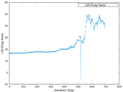
Figure 13: Left: the mesh generated from DWR-based adaptation. Right: the Mach isoline of the optimized airfoil.

We conducted the optimization task of maximizing the lift-drag ratio of NACA0012 with Mach number $0.8$ and attack angle $1.25^{\circ}$ as well. The value of the lift-drag ratio gets raised from $16.488$ to $48.916$. Optimizing for the lift-drag ratio poses greater challenges than solely focusing on drag due to the complex calculation of lift. Firstly, the calculation of lift is more complicated compared with drag. Evidence from our previous experiments and other researchers [10] have shown that the convergence curve of lift during the calculation is oscillatory. This may be caused by the weaker regularity of the dual solution for the lift coefficient. Even though dual consistency has been considered, such a problem has not been fully figured out. Secondly, the DWR-based mesh adaptation method can not be generalized to the lift-drag ratio easily. Then, the accuracy of the target functional gets influenced a lot. Multi-mesh method[52] can be applied to solve the lift and drag respectively. However, it will bring additional difficulties to the PDE solver.

Currently, we pay more attention to the drag calculation since the denominator demands higher accuracy in a fractional calculation. The mesh generated from DWR-based adaptation as shown in Figure 14 is adopted to calculate the lift-drag ratio. Our experiments, illustrated in Figure 13, highlight potential issues with data anomalies that can arise when the framework for solving the designated functional is not sufficiently accurate. Such inaccuracies can lead to erroneous signals that adversely affect the policy update of the agent. Moreover, it is evident that there is a need for a more task-specific design of the reward functional. The optimization process depicted in Figure 13 underwent an extensive period of exploration to identify a viable direction for improvement. Although the optimized shape has a lift-drag ratio nearly three times than the original one, it seems this airfoil shape does not represent the intended airfoil design. The anticipated shape could potentially exhibit even greater deviations. Thus, the agent should explore more potential shapes to generate the best geometry, which will consume time significantly longer than the current experiment. While the current PDE solver has already been a highly efficient one, an increase of magnitude with respect to the wall time is tough. Multi-agent exploration framework should be constructed in the future to enhance this algorithm. Shock waves present both on the lower and upper side of the airfoil from the result in Figure 14 which may be attributed to the problem that the value of the lift-drag ratio during the optimization process stopped around $45$. In order to develop a task-specific design algorithm for the lift-drag calculation, we need to pay attention to the pressure distribution along the geometry as well. Besides, the analysis should be developed further to ensure the equivalence of the optimization objective.

Figure 14: Left: the Mach isoline of the initial airfoil. Right: the Mach isoline of the optimized airfoil.

7 Conclusion

In this work, we present a novel framework that integrates reinforcement learning with goal-oriented PDEs-based systems for airfoil shape optimization. Operating within the challenging environment of unstructured meshes, we encountered significant obstacles such as mesh tangling, the management of high-dimensional state representations, and the occurrence of non-smooth geometries. To address these issues, we developed a suite of mesh recovery techniques aimed at improving mesh quality.

It is important to highlight that the reinforcement learning approach was meticulously tailored to align with the intrinsic motivation behind the optimization objectives. The design of the neural network was carefully crafted to meet these specific requirements while circumventing the potential for gradient vanishing issues. Moreover, we established a nuanced system of rewards and penalties to facilitate the interactive optimization process. Upon conducting experimental validations of shape optimization, our findings demonstrate that the proposed framework is adept at managing simulations with precisely calculated objective functions.

However, due to the current theoretical limitations of DWR-based mesh adaptation methods, more complex target functionals have not yet been further explored. Looking forward, we aim to integrate advanced techniques, such as the multi-mesh method for tackling more intricate target functionals and employing multi-agent strategies for enhanced exploration efficiency. We believe that multi-agent systems can achieve a deeper integration with traditional optimization algorithms based on adjoint equations, leading to more efficient exploration patterns. Furthermore, the adoption of various acceleration techniques, including the incorporation of additional learning modules, parallelization strategies, and more efficient network architectures, represents a promising direction for future development.

References

- [1] Joaquim RRA Martins and Andrew B Lambe. Multidisciplinary design optimization: a survey of architectures. AIAA journal, 51(9), 2013.
- [2] Siva K Nadarajah and Antony Jameson. Optimum shape design for unsteady flows with time-accurate continuous and discrete adjoint method. AIAA journal, 45(7), 2007.
- [3] P Panagiotou and K Yakinthos. Aerodynamic efficiency and performance enhancement of fixed-wing uavs. Aerospace Science and Technology, 99:105575, 2020.
- [4] Jeffrey P Slotnick, Abdollah Khodadoust, Juan Alonso, David Darmofal, William Gropp, Elizabeth Lurie, and Dimitri J Mavriplis. CFD vision 2030 study: a path to revolutionary computational aerosciences. Technical report, 2014.
- [5] Mohamed A Bouhlel and Joaquim RRA Martins. Gradient-enhanced kriging for high-dimensional problems. Engineering with Computers, 35(1), 2019.
- [6] David M Deaven and Kai-Ming Ho. Molecular geometry optimization with a genetic algorithm. Physical review letters, 75(2):288, 1995.
- [7] Antony Jameson. Aerodynamic design via control theory. Journal of scientific computing, 3:233–260, 1988.
- [8] James Reuther, Antony Jameson, James Farmer, Luigi Martinelli, and David Saunders. Aerodynamic shape optimization of complex aircraft configurations via an adjoint formulation. In 34th aerospace sciences meeting and exhibit, page 94, 1996.
- [9] Krzysztof Fidkowski and David Darmofal. Review of output-based error estimation and mesh adaptation in computational fluid dynamics. AIAA journal, 49(4):673–694, 2011.
- [10] Vít Dolejší, Ondřej Bartoš, and Filip Roskovec. Goal-oriented mesh adaptation method for nonlinear problems including algebraic errors. Computers & Mathematics with Applications, 93:178–198, 2021.
- [11] Ralf Hartmann and Tobias Leicht. Generalized adjoint consistent treatment of wall boundary conditions for compressible flows. Journal of Computational Physics, 300:754–778, 2015.
- [12] Xucheng Meng, Yaguang Gu, and Guanghui Hu. A fourth-order unstructured NURBS-enhanced finite volume WENO scheme for steady Euler equations in curved geometries. Communications on Applied Mathematics and Computation, pages 1–28, 2021.
- [13] Xucheng Meng and Guanghui Hu. A nurbs-enhanced finite volume method for steady euler equations with goal-oriented -adaptivity. Communications in Computational Physics, 32:490–523, 06 2022.
- [14] Lorenz T Biegler, Omar Ghattas, Matthias Heinkenschloss, and Bart van Bloemen Waanders. Large-scale pde-constrained optimization: an introduction. In Large-Scale PDE-Constrained Optimization, pages 3–13. Springer, 2003.
- [15] Grégoire Allaire, François Jouve, and Anca-Maria Toader. Structural optimization using sensitivity analysis and a level-set method. Journal of computational physics, 194(1):363–393, 2004.
- [16] Jichao Li, Xiaosong Du, and Joaquim RRA Martins. Machine learning in aerodynamic shape optimization. Progress in Aerospace Sciences, 134:100849, 2022.
- [17] Wei Chen, Kevin Chiu, and Mark D Fuge. Airfoil design parameterization and optimization using bézier generative adversarial networks. AIAA journal, 58(11):4723–4735, 2020.
- [18] Wei Chen, Kevin Chiu, and Mark Fuge. Aerodynamic design optimization and shape exploration using generative adversarial networks. In AIAA SciTech Forum, San Diego, USA, Jan 2019. AIAA.
- [19] Kazuo Yonekura and Katsuyuki Suzuki. Data-driven design exploration method using conditional variational autoencoder for airfoil design. Structural and Multidisciplinary Optimization, 64(2):613–624, 2021.
- [20] Kai Arulkumaran, Marc Peter Deisenroth, Miles Brundage, and Anil Anthony Bharath. Deep reinforcement learning: A brief survey. IEEE Signal Processing Magazine, 34(6):26–38, 2017.
- [21] Volodymyr Mnih, Koray Kavukcuoglu, David Silver, Andrei A Rusu, Joel Veness, Marc G Bellemare, Alex Graves, Martin Riedmiller, Andreas K Fidjeland, Georg Ostrovski, et al. Human-level control through deep reinforcement learning. nature, 518(7540):529–533, 2015.
- [22] Thomas Duriez, Steven L Brunton, and Bernd R Noack. Machine learning control-taming nonlinear dynamics and turbulence, volume 116. Springer, 2017.
- [23] Jean Rabault, Miroslav Kuchta, Atle Jensen, Ulysse Réglade, and Nicolas Cerardi. Artificial neural networks trained through deep reinforcement learning discover control strategies for active flow control. Journal of fluid mechanics, 865:281–302, 2019.
- [24] Guanghui Hu, Ruo Li, and Tao Tang. A robust high-order residual distribution type scheme for steady Euler equations on unstructured grids. Journal of Computational Physics, 229(5):1681–1697, 2010.
- [25] Guanghui Hu, Ruo Li, and Tao Tang. A robust WENO type finite volume solver for steady Euler equations on unstructured grids. Communications in Computational Physics, 9(3):627–648, 2011.
- [26] Guanghui Hu. An adaptive finite volume method for 2D steady Euler equations with WENO reconstruction. Journal of Computational Physics, 252:591–605, 2013.
- [27] Amanda Lampton, Adam Niksch, and John Valasek. Reinforcement learning of a morphing airfoil-policy and discrete learning analysis. Journal of Aerospace Computing, Information, and Communication, 7(8):241–260, 2010.
- [28] Jonathan Viquerat, Jean Rabault, Alexander Kuhnle, Hassan Ghraieb, Aurélien Larcher, and Elie Hachem. Direct shape optimization through deep reinforcement learning. Journal of Computational Physics, 428:110080, 2021.
- [29] Xinghui Yan, Jihong Zhu, Minchi Kuang, and Xiangyang Wang. Aerodynamic shape optimization using a novel optimizer based on machine learning techniques. Aerospace Science and Technology, 86:826–835, 2019.
- [30] Guanghui Hu, Xucheng Meng, and Nianyu Yi. Adjoint-based an adaptive finite volume method for steady Euler equations with non-oscillatory k-exact reconstruction. Computers & Fluids, 139:174–183, 2016.
- [31] Guanghui Hu and Nianyu Yi. An adaptive finite volume solver for steady Euler equations with non-oscillatory k-exact reconstruction. Journal of Computational Physics, 312:235–251, 2016.
- [32] Jingfeng Wang and Guanghui Hu. Towards the efficient calculation of quantity of interest from steady Euler equations I: a dual-consistent DWR-based h-adaptive Newton-GMG solver. arXiv preprint arXiv:2302.14262, 2023.
- [33] Jingfeng Wang and Guanghui Hu. Towards the efficient calculation of quantity of interest from steady euler equations ii: a cnns-based automatic implementation. arXiv preprint arXiv:2308.07140, 2023.
- [34] Yann LeCun, Yoshua Bengio, and Geoffrey Hinton. Deep learning. nature, 521(7553):436–444, 2015.
- [35] Marian Nemec and Michael Aftosmis. Toward automatic verification of goal-oriented flow simulations. Technical Report NASA/TM-2014-218386, 2014.
- [36] Andrew A Johnson and Tayfun E Tezduyar. Mesh update strategies in parallel finite element computations of flow problems with moving boundaries and interfaces. Computer methods in applied mechanics and engineering, 119(1-2):73–94, 1994.
- [37] Thomas P Dussauge, Woong Je Sung, Olivia J Pinon Fischer, and Dimitri N Mavris. A reinforcement learning approach to airfoil shape optimization. Scientific Reports, 13(1):9753, 2023.
- [38] Giampietro Carpentieri, Barry Koren, and Michel JL van Tooren. Adjoint-based aerodynamic shape optimization on unstructured meshes. Journal of Computational Physics, 224(1):267–287, 2007.
- [39] Qiuyi Chen, Phillip Pope, and Mark Fuge. Learning Airfoil Manifolds with Optimal Transport.
- [40] F Pérez-Arribas and I Castañeda-Sabadell. Automatic modelling of airfoil data points. Aerospace Science and Technology, 55:449–457, 2016.
- [41] Ian Dewancker, Michael McCourt, and Scott Clark. Bayesian optimization for machine learning: A practical guidebook. arXiv preprint arXiv:1612.04858, 2016.
- [42] Kaiming He, Xiangyu Zhang, Shaoqing Ren, and Jian Sun. Deep residual learning for image recognition. In Proceedings of the IEEE conference on computer vision and pattern recognition, pages 770–778, 2016.
- [43] Günter Klambauer, Thomas Unterthiner, Andreas Mayr, and Sepp Hochreiter. Self-normalizing neural networks. Advances in neural information processing systems, 30, 2017.
- [44] Martín Abadi, Paul Barham, Jianmin Chen, Zhifeng Chen, Andy Davis, Jeffrey Dean, Matthieu Devin, Sanjay Ghemawat, Geoffrey Irving, Michael Isard, et al. Tensorflow: a system for large-scale machine learning. In Osdi, volume 16, pages 265–283. Savannah, GA, USA, 2016.
- [45] Antony Jameson and James Reuther. Control theory based airfoil design using the euler equations. 10 1994.
- [46] Ruo Li, Xin Wang, and Weibo Zhao. A multigrid block LU-SGS algorithm for Euler equations on unstructured grids. Numerical Mathematics: Theory, Methods and Applications, 1:92–112, 2008.
- [47] David Venditti and David Darmofal. Adjoint error estimation and grid adaptation for functional outputs: Application to quasi-one-dimensional flow. Journal of Computational Physics, 164(1):204–227, 2000.
- [48] David A Venditti and David L Darmofal. Grid adaptation for functional outputs: application to two-dimensional inviscid flows. Journal of Computational Physics, 176(1):40–69, 2002.
- [49] Marian Nemec and Michael Aftosmis. Adjoint error estimation and adaptive refinement for embedded-boundary cartesian meshes. In 18th AIAA computational fluid dynamics conference, page 4187, 2007.
- [50] Toru Yamahara, Kazuhiro Nakahashi, and Hyoungjin Kim. Adaptive mesh refinement using viscous adjoint method for single-and multi-element airfoil analysis. International Journal of Aeronautical and Space Sciences, 18(4):601–613, 2017.
- [51] Vít Dolejší and Georg May. An anisotropic hp-mesh adaptation method for time-dependent problems based on interpolation error control. Journal of Scientific Computing, 95(2):36, 2023.
- [52] Yang Kuang, Yedan Shen, and Guanghui Hu. Towards chemical accuracy using a multi-mesh adaptive finite element method in all-electron density functional theory. arXiv preprint arXiv:2310.15651, 2023.
- [53] Ruo Li. On multi-mesh h-adaptive methods. Journal of Scientific Computing, 24:321–341, 2005.
- [54] Richard Bellman. A markovian decision process. Journal of mathematics and mechanics, pages 679–684, 1957.
- [55] Hado Van Hasselt, Arthur Guez, and David Silver. Deep reinforcement learning with double q-learning. In Proceedings of the AAAI conference on artificial intelligence, volume 30, 2016.
- [56] John Schulman, Filip Wolski, Prafulla Dhariwal, Alec Radford, and Oleg Klimov. Proximal policy optimization algorithms. arXiv preprint arXiv:1707.06347, 2017.
- [57] Scott Fujimoto, Herke Hoof, and David Meger. Addressing function approximation error in actor-critic methods. In International conference on machine learning, pages 1587–1596. PMLR, 2018.
- [58] Diederik P Kingma and Max Welling. Auto-encoding variational bayes. arXiv preprint arXiv:1312.6114, 2013.
- [59] Na Lei, Kehua Su, Li Cui, Shing-Tung Yau, and Xianfeng David Gu. A geometric view of optimal transportation and generative model. Computer Aided Geometric Design, 68:1–21, 2019.