A robust shifted proper orthogonal decomposition:
Proximal methods for decomposing flows with multiple transports

Abstract

We present a new methodology for decomposing flows with multiple transports that further extends the shifted proper orthogonal decomposition (sPOD). The sPOD tries to approximate transport-dominated flows by a sum of co-moving data fields. The proposed methods stem from sPOD but optimize the co-moving fields directly and penalize their nuclear norm to promote low rank of the individual data in the decomposition. Furthermore, we add a robustness term to the decomposition that can deal with interpolation error and data noises. Leveraging tools from convex optimization, we derive three proximal algorithms to solve the decomposition problem. We report a numerical comparison with existing methods against synthetic data benchmarks and then show the separation ability of our methods on 1D and 2D incompressible and reactive flows. The resulting methodology is the basis of a new analysis paradigm that results in the same interpretability as the POD for the individual co-moving fields.

Keywords: forward-backward, transport phenomena, proper orthogonal decomposition, vortex shedding, reactive flows

1 Introduction

Modeling of flow in time-varying geometries or of expanding reaction waves poses major mathematical challenges due to the inherent difficulty of efficiently reducing the number of degrees of freedom (DOF). For instance, high-fidelity simulations on massively parallel computing architectures are usually performed in multi-query applications to understand the flight mechanics of an insect or the spread of a fire [66, 68] for a range of parameters, e.g. Reynolds numbers or burning rates. These simulations are very costly due to the tremendous amount of DOFs in the system. A common approach is to reduce the DOFs with the help of the proper orthogonal decomposition (POD) and Galerkin projections, originally introduced in [46, 6]. For a review of the POD-Galerkin model order reduction (MOR) approach, we refer to [5, 41]). However, POD-Galerkin projects the studied system onto a reduced linear subspace, which is often not able to capture the full dynamics of the system. Therefore, it introduces large approximation errors. In particular, in the presence of moving quantities or structures with small support, the POD-Galerkin approach breaks down, which limits its applicability to study transport-dominated flows.

In this work, we build on the shifted POD method (sPOD) [59], which enriches the reduced linear subspace of the POD by moving it using the transport of the system and therefore achieves better approximation errors. Although multiple gradient-based optimization algorithms for the sPOD already exist in the literature [59, 9, 58], the method needs to be generalized to achieve a better separation and a more accurate description of the transport phenomena, in particular for multiple transports. We thus derive in this work, three proximal algorithms that generalize the existing framework.

1.1 Model order reduction for transport-dominated systems

Model order reduction for transport-dominated systems has been widely studied in the literature (see [55] for a review), since it is one of the key challenges, for instance, in reducing combustion systems [29]. Transport-dominated systems are especially challenging because traditional MOR based on low-dimensional linear subspace approximations breaks down. This phenomenon is known as the Kolmogorov $n$-width barrier and was first theoretically studied in [52, 25]. For linear transports, the Kolmogorov $n$-width decay was recently proven not to be a problem of the PDE itself; it depends on the smoothness of the initial condition and the boundary values [1]. However, transport-dominated systems do not only occur in linear advected systems but, for instance, also in combustion systems [29, 16, 10, 40] flows around moving geometries [39, 36, 35], kinetic systems [34, 7], and moment models [33].

To overcome the slow decay of the approximation errors in transport-dominated systems with the approximation dimension, a description that adapts to the transport of the system can be used. One can subdivide the literature mainly into three different groups. The first group builds on the expressivity of neural networks [43, 22, 23, 31, 28, 63, 69]. More specifically, the authors in [34, 22, 43, 31] rely on an autoencoder (AE) structures. Unfortunately, AEs often compromise the structural insights, such as the interpretability of the identified structures and the optimality of the resulting description. Nonetheless, physics-informed neural networks (PINNs) [31] can still provide an understanding of the internal low-dimensional dynamics. Furthermore, AE neural networks are used in [34] to identify and interpret the correspondence between the intrinsic variables and the learned structures in Boltzmann equations. A combination of classical reduction methods like POD or kernel POD with neural networks has also been studied [23, 28, 63, 69]. It allows for a better quantification of the errors [15], which is usually not possible with classical AE.

The second group uses online-adaptive basis methods [32, 54, 56] that compute the linear approximation space locally and adaptively in time. Consequently, they fully omit the costly data sampling stage of classical MOR. However, [33] shows that the construction and update of the basis in each time step lead to a significant overhead and computational cost compared to the classical approach in which the reduced order model (ROM) is set up a priori based on the data generated by the original PDE system.

The last group, that includes sPOD, builds on the idea of transport compensation [21, 40, 38, 30, 50, 59, 60, 62, 65, 70] which aims at enhancing the approximation of a linear description by aligning the parameters or time-dependent structures with the help of suited transforms. Apart of sPOD, other methods from tis group include symmetry reduction that combines symmetries, like translation invariance of the underlying PDE, with a POD reduction approach [62, 21]. This approach was proved to be a special case of the sPOD in [9]. In [60] transported subspaces are used, by making explicit use of characteristics of the hyperbolic PDEs or by tracking the front of the reduced system [38, 40]. Another approach uses a space-time registration to align the subspace to local features in the flow [65]. In [70], transformed snapshots ares used in place of the POD. Lastly, invertible parameter-dependent mappings of the flow domain are used in [50] to allow parameter-dependent deformations in the ROM.

The sPOD enjoys a close connection to the snapshot POD [64], which is not only a data reduction method, but also a tool for the analysis of fluid systems transient dynamics in vortex shedding [49], coherent structures in swirling jets [51], or stability analysis [6]. In fact, the sPOD can be seen as a natural extension of the POD that shares a similar interpretability after the isolation of the individual co-moving structures. Such a close connection to the studied problem physics makes the sPOD an attractive method to develop further.

1.2 State of the art

The sPOD was first introduced in [59] based on a heuristic optimization of a residuum. The method builds on the idea that a single traveling wave or moving localized structure can be perfectly described by its wave profile and a time-dependent shift. Therefore, the sPOD decomposes transport fields by shifting the data field in multiple co-moving frames, in which the different waves are stationary and can be described with a few spatial basis functions determined by the POD. The sPOD was then further developed in [11, 10, 9, 58]. More specifically, the sPOD was studied in its space-time continuous formulation in [9] before being discretized and solved as an optimization problem. The formulation was proven to have a solution under the assumption that the involved transformations are smooth. This formulation was later generalized in [11] to include the optimization of the shifts using initial shifts that are already close to the optimum. Nevertheless, the presented decomposition approach has not been used in the context of efficient ROMs. A first application of sPOD for efficient ROMs is given in [10] but the method relies on cutting the domain such that two distinct co-moving systems can be found and separated. Furthermore, the decomposition relies on choosing the ranks of each co-moving field beforehand. For complicated systems, this choice is often critical for the quality of the decomposition.

In contrast, [58] proposes a discrete optimization problem based on the decay of singular values in each co-moving field. The problem shares more similarities with the discrete space implementation of the POD, which technically boils down to a singular value decomposition (SVD). Minimizing the nuclear norm of the co-moving fields results in a non-strictly convex problem that is easy to solve under the assumption of the convexity of the transport operators. Additionally, the choice of the ranks in each co-moving field is performed during the minimization. Unfortunately, the gradient-based optimization approach presented in [58] shows slow convergence, due to the non-smoothness of the nuclear norm. Furthermore, this method is not robust to noise, as the exact ranks of synthetic test cases could not be estimated correctly. In this work, we proposes a method to circumvent these two impediments.

1.3 Contribution and outline

Our contribution is as follows:

1. Three proximal algorithms are proposed to solve the sPOD formulation, two of them enjoy desirable theoretical properties such as descent property and convergence to a critical point, even in a non-convex setting. These properties are important since, in contrast with [58], the convexity of the transport operators is not assumed.

2. An additional noise term can be included to capture interpolation noise or artifacts in the data to accurately predict the ranks of the system.

3. A comparison of our algorithms with existing ones is conducted.

4. Applications of our methods to realistic 2D incompressible and 2D reactive flow are presented.

The main novelty of this work is to show that the new algorithms lead to a better and more efficient separation of the physical phenomena, which opens research for building surrogate models of individual systems.

The article is organized as follows: Section 2 introduces the sPOD problem in the continuous and discrete settings with our proposed generalization towards a robust decomposition. In Section 3, we reformulate the discrete sPOD problem and leverage tools from convex optimization to design three algorithms that solve the latter problem. Results of numerical experiments are presented in Section 4 and Section 5 concludes.

Notation. Bold upper case letters denote matrices, bold lower case letters denote vectors, and lowercase letters denote scalars. The notation $\left\lVert.\right\rVert_{*}$ and $\left\lVert.\right\rVert_{\mathrm{F}}$ denote the nuclear and the Frobenius norms of a matrix respectively. The set $\llbracket 1,N\rrbracket$ denotes the set of natural integers from $1$ to $N$. In the following, we refer to a critical point for a function $f$ as a point where its subdifferential contains $0$.

2 Shifted POD

The sPOD is a non-linear decomposition of a transport-dominated field $q(x,t)$ into multiple co-moving structures $\{q^{k}(x,t)\}_{k\in\llbracket 1,K\rrbracket}$ with their respective transforms $\{\mathcal{T}^{k}\}_{k\in\llbracket 1,K\rrbracket}$

$$q(x,t)=\sum_{k=1}^{K}\mathcal{T}^{k}q^{k}(x,t)\,.$$ (1)

where $K$ is the number of co-moving frames. The transforms are usually chosen such that the resulting co-moving structure can be described efficiently with the help of a dyadic decomposition

$$q^{k}(x,t)\approx\sum_{r=1}^{R_{k}}\alpha^{k}_{r}(x,t)\phi^{k}_{r}(x,t)\,,$$ (2)

where $R_{k}$ is the co-moving rank. Hence, the total number of DOFs in the approximation is $R=\sum_{k=1}^{K}R_{k}$. The operator $\mathcal{T}^{k}$ transforms the co-moving coordinate frame in the reference frame while its inverse $\mathcal{T}^{-k}:=(\mathcal{T}^{k})^{-1}$ transforms it back. In this work, the operators are assumed to be smoothly dependent on time and each operator implements a shift $\Delta^{k}(t)$ defined as

$$\mathcal{T}^{k}q^{k}(x,t)=q^{k}(x-\Delta^{k}(t),t)\quad,\quad\mathcal{T}^{-k}q^{k}(x,t)=q^{k}(x+\Delta^{k}(t),t)\,.$$ (3)

It is straightforward to also include additional parameter dependencies in the transforms as shown in [10, 16]. Furthermore, the transformations can also include rotations [36, 35] or other diffeomorphic mappings [47]. In general, a single transformation is assumed to be at least piecewise differentiable in time and diffeomorphic. Nevertheless, the decomposition in the sense of eq. 1 is not unique in general, since multiple diffeomorphic mappings are involved.

Usually, MOR is performed on a discrete data set. Without loss of generality, we assume one spatial and one temporal dimension for the purpose of the sPOD description. Thus, the data set includes $M$ spatial grid points $\{x_{m}\}$ and $N$ time grid points $\{t_{n}\}$. This discretization results in the construction of a snapshot matrix $\mathbf{Q}$

$$\mathbf{Q} =\left[\mathbf{q}(t_{1}),\dots,\mathbf{q}(t_{N})\right]\in\mathbb{R}^{M\times N},$$

$$\text{with}\quad\mathbf{q}(t) =[q(x_{1},t),\dots,q(x_{M},t)]^{\top}\in\mathbb{R}^{M}\,.$$

Therefore, the shift transformation eq. 3 now reads

$$\mathcal{T}^{k}\mathbf{Q} =\left[\mathcal{T}^{k}\mathbf{q}(t_{1}),\dots,\mathcal{T}^{k}\mathbf{q}(t_{N})\right]\in\mathbb{R}^{M\times N},$$

$$\text{with}\quad\mathcal{T}^{k}\mathbf{q}(t) =[q(x_{1}-\Delta^{k}(t),t),\dots,q(x_{M}-\Delta^{k}(t),t)]\in\mathbb{R}^{M}\,.$$

Since $\tilde{x}=x_{m}-\Delta(t)$ may not lie on the grid, it is interpolated from neighboring grid points. In this work, the interpolation is performed with Lagrange polynomials of degree $5$, which introduces an interpolation error of order $\mathcal{O}(h^{6})$ [37]. Note that, with a slight abuse of notation, we use $\mathcal{T}^{k}$ to denote eq. 3 and its approximation using Lagrange interpolation. In the remainder of the text, we assume an equidistant, periodic grid with constant lattice spacing. This is not a restriction of the problem, as non-periodic domains can be realized by padding the domain such that no data is lost after shifting it [58, 35].

After discretization, Equations eq. 2 and eq. 1 result in the following non-linear matrix decomposition

$$\mathbf{Q}\approx\bm{\tilde{\mathbf{Q}}}\stackrel{{\scriptstyle\mbox{\footnotesize def}}}{{=}}\sum_{k=1}^{K}\mathcal{T}^{k}\mathbf{Q}^{k}\,.$$ (4)

In this discrete setting, we optimize on the co-moving data fields $\mathbf{Q}^{k}\in\mathbb{R}^{M\times N}$, that are further decomposed by using an SVD

$$(\forall k\in\llbracket 1,K\rrbracket)\quad\mathbf{Q}^{k}=\bm{\Psi}^{k}\bm{\Sigma}^{k}(\mathbf{V}^{k})^{\top}\,.$$ (5)

Here, $\bm{\Sigma}^{k}=\operatorname{diag}{(\sigma_{1}^{k},\dots,\sigma_{P}^{k})}$ with $P=\min(M,N)$ is a diagonal matrix containing the singular values $\sigma_{1}^{k}\geq\sigma_{2}^{k}\geq\dots\geq\sigma_{P}^{k}$ while $\bm{\Psi}^{k}\in\mathbb{R}^{M\times P}$ and $\mathbf{V}^{k}\in\mathbb{R}^{N\times P}$ are orthogonal matrices containing the left and right singular vectors, respectively. The POD modes are contained in the first $R_{k}$ columns of $\mathbf{\Psi}^{k}=[\phi_{p}^{k}(x_{m})]_{mp}\in\mathbb{R}^{M\times P}$. The approximation dimensions $\{R_{k}\}_{k}$ need to be estimated in an adequate manner. For maximal efficiency, we aim for a small number of modes $R=\sum_{k=1}^{K}R_{k}\ll N$. Therefore, we can formulate the search of a POD decomposition shown in eq. 4 as the following optimization problem

$$\underset{\begin{subarray}{c}{\{\mathbf{Q}^{k}\}_{k}}\end{subarray}}{\mathrm{minimize}}\;\;\sum_{k=1}^{K}\operatorname{rank}(\mathbf{Q}^{k})\quad\text{s.t. }\mathbf{Q}=\sum_{k=1}^{K}\mathcal{T}^{k}\mathbf{Q}^{k}\,.$$ (6)

As minimizing over the rank of a matrix is NP-hard [57], we substitute the nuclear norm for the rank function, the former being the convex hull of the latter. Problem eq. 6 is thus relaxed into

$$\underset{\begin{subarray}{c}{\{\mathbf{Q}^{k}\}_{k}}\end{subarray}}{\mathrm{minimize}}\;\;\sum_{k=1}^{K}\left\lVert\mathbf{Q}^{k}\right\rVert_{*}\quad\text{s.t. }\mathbf{Q}=\sum_{k=1}^{K}\mathcal{T}^{k}\mathbf{Q}^{k}\,.$$ (7)

This relaxation of the rank function is common in robust PCA [44, 45, 17]. However, relaxing the sum of the ranks to the sum of the nuclear norms is not a tight relaxation: indeed, the convex hull of a sum of functions is not equal to the sum of the convex hulls of each function in general.

Optimization Problem eq. 7 was already formulated in [58] and it was solved based on a Broyden–Fletcher–Goldfarb–Shanno method with an inexact line search designed for non-smooth optimization problems. Nonetheless, the convergence was observed to be slow, rendering the method inefficient in practice. Furthermore, convergence to the exact ranks could not be achieved due to the interpolation noise introduced by the discrete transport operators. To circumvent the latter issue, we introduce an extra term $\mathbf{E}\in\mathbb{R}^{M\times N}$ in the sPOD decomposition

$$\mathbf{Q}=\sum_{k=1}^{K}\mathcal{T}^{k}(\mathbf{Q}^{k})+\mathbf{E}\,,$$ (8)

in order to capture both the interpolation noise and the noise that could corrupt the data. The resulting optimization problem thus reads

$$\underset{\begin{subarray}{c}{\{\mathbf{Q}^{k}\}_{k},\mathbf{E}}\end{subarray}}{\mathrm{minimize}}\;\;\sum_{k=1}^{K}\lambda_{k}\left\lVert\mathbf{Q}^{k}\right\rVert_{*}+\lambda_{K+1}\left\lVert\mathbf{E}\right\rVert_{1}\quad\text{s.t. }\mathbf{Q}=\sum_{k=1}^{K}\mathcal{T}^{k}\mathbf{Q}^{k}+\mathbf{E}\,,$$ (9)

where $\left\lVert\mathbf{E}\right\rVert_{1}=\sum_{ij}|\mathbf{E}_{ij}|$ corresponds to the $\ell_{1}$-norm of the vectorization of $\mathbf{E}$ and $\{\lambda_{k}\}_{k\in\llbracket 1,K+1\rrbracket}$ are positive scalar parameters that can be tuned to yield different weights to the terms in the objective function. Similar to the robust PCA, solving eq. 9 aims at decomposing $\mathbf{Q}=\bm{\tilde{\mathbf{Q}}}+\mathbf{E}$ into a low rank matrix $\bm{\tilde{\mathbf{Q}}}$ and a sparse noisy matrix $\mathbf{E}$. A visualization of this decomposition is shown in fig. 1.

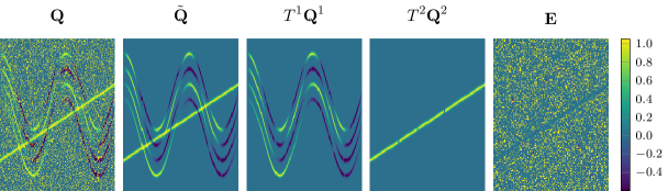
Figure 1: Illustration of the robust sPOD. The noise is computed by randomly setting 12.5% of the input entries of $\mathbf{Q}$ to $1$. The input data $\mathbf{Q}$ and its decomposition into a low-rank part $\bm{\tilde{\mathbf{Q}}}=\mathcal{T}^{1}\mathbf{Q}^{1}+\mathcal{T}^{2}\mathbf{Q}^{2}$ as well as the noise matrix $\mathbf{E}$ are displayed from left to right.

3 Low-rank decomposition of the snapshot matrix

This section describes two formulations of eq. 9 as well as the design of three algorithms that, given a snapshot matrix $\mathbf{Q}$ and the transport operators $\{\mathcal{T}^{k}\}_{k\in\llbracket 1,K\rrbracket}$, return low-rank estimates of the co-moving fields $\{\mathbf{Q}^{k}\}_{k\in\llbracket 1,K\rrbracket}$ as well as the residual error $\mathbf{E}$.

3.1 Unconstrained formulation

We first write Problem eq. 9 as the following unconstrained optimization problem

$$\underset{\begin{subarray}{c}{\{\mathbf{Q}^{k}\}_{k},\mathbf{E}}\end{subarray}}{\mathrm{minimize}}\;\;\quad\underbrace{\frac{1}{2}\left\lVert\mathbf{Q}-\sum_{k=1}^{K}\mathcal{T}^{k}\mathbf{Q}^{k}-\mathbf{E}\right\rVert_{\mathrm{F}}^{2}}_{\stackrel{{\scriptstyle\mbox{\footnotesize def}}}{{=}}f(\{\mathbf{Q}^{k}\}_{k},\mathbf{E})}+\sum_{k=1}^{K}\underbrace{\lambda_{k}\left\lVert\mathbf{Q}^{k}\right\rVert_{*}}_{\stackrel{{\scriptstyle\mbox{\footnotesize def}}}{{=}}g_{k}(\mathbf{Q}^{k})}+\underbrace{\lambda_{K+1}\left\lVert\mathbf{E}\right\rVert_{1}}_{\stackrel{{\scriptstyle\mbox{\footnotesize def}}}{{=}}\tilde{g}(\mathbf{E})}\,,$$ (10)

where $f$ is the data fitting term that forces the optimization variables to fit the snapshot matrix $\mathbf{Q}$, $\{g_{k}\}_{k\in\llbracket 1,K\rrbracket}$ promotes low-rank estimates of the $\{\mathbf{Q}^{k}\}_{k}$, and $\tilde{g}$ promotes sparse residual error $\mathbf{E}$. Note that problem eq. 10 has a solution since its objective function is lower semi-continuous and coercive. Therefore, the set of its minimizers is a non-empty compact set.

We define the regularization term $g$ such that $g(\{\mathbf{Q}^{k}\}_{k},\mathbf{E})=\sum_{k=1}^{K}g_{k}(\mathbf{Q}^{k})+\tilde{g}(\mathbf{E})$. Hence, by denoting $\mathbf{x}={(\mathbf{Q}^{1},\dots,\mathbf{Q}^{K},\mathbf{E})}^{\top}$ the vector of optimization variables, problem eq. 10 reads

$$\min_{\mathbf{x}}\quad F(\mathbf{x})\stackrel{{\scriptstyle\mbox{\footnotesize def}}}{{=}}f(\mathbf{x})+g(\mathbf{x})\,.$$ (11)

The function $f$ is a $\mathcal{C}^{1}$ non-convex function with $\beta$-Lipschitz gradient while $g$ is a proper lower semi-continuous, convex, non-smooth and separable function. The objective function $F$ is bounded from below by $0$ since it is the sum of two non-negative functions, $f$ and $g$. Splitting algorithms are well-appropriate to solve problems in the form of eq. 11 [19].

3.2 Joint proximal gradient method

Splitting problems such as eq. 11 have been extensively studied in the convex optimization literature (see [3] and references therein) and an efficient algorithm to solve them is the Forward-Backward (FB) algorithm, also known as the proximal gradient method [4]. The FB method is an iterative algorithm whose iterations are composed by a gradient step (or forward step) on the smooth term, here $f$, and a proximal step (or backward step) on the non-smooth term, here $g$. A single step at iteration $t$ can be summarized as follows

$$\mathbf{x}^{(t+1)}\quad\longleftarrow\quad{\operatorname{prox}}_{\alpha g}\left(\mathbf{x}^{(t)}-\alpha\nabla f(\mathbf{x}^{(t)})\right)\,,$$ (12)

where the superscript $t$ refers to the current iteration, $\alpha$ is the stepsize, and $\operatorname{prox}$ is the proximal operator which is uniquely defined for a proper lower semi-continuous convex function $h:\mathbb{R}^{N}\rightarrow\mathbb{R}^{N}$ as

$${\operatorname{prox}}_{h}:\mathbf{x}\mapsto\operatorname*{arg\,min}_{\mathbf{y}\in\mathbb{R}^{N}}h(\mathbf{y})+\frac{1}{2}\left\lVert\mathbf{y}-\mathbf{x}\right\rVert_{2}^{2}\,.$$

The proximity operator was introduced in the early work [48] and can be viewed as a generalization of the projection onto a convex set. Indeed, the proximity operator of an indicator function on a convex set is equal to the projection on this set. Moreover, the proximity operator enjoys many projection-like properties such as non-expansiveness. See [3] for an exhaustive presentation of the proximity operator.

In order to apply the FB algorithm to solve eq. 10, we need to perform the iteration eq. 12, i.e. to compute the gradient of $f$ as well as the proximity operator of $g$. Using the definition of the gradient, we have that $\nabla f(\mathbf{x})={(\nabla_{\mathbf{Q}^{1}}f(\mathbf{x}),\dots,\nabla_{\mathbf{E}}f(\mathbf{x}))}^{\top}$. The computation of the partial gradients is performed in [58] and yields

$$(\forall k\in\llbracket 1,K\rrbracket)\quad\nabla_{\mathbf{Q}^{k}}f(\mathbf{x})=-\mathcal{T}^{-k}\mathbf{R}\quad\text{and}\qquad\nabla_{\mathbf{E}}f(\mathbf{x})=-\mathbf{R}\,,$$

where $\mathbf{R}$ is the residual of the approximation $\mathbf{R}=\mathbf{Q}-\sum_{k=1}^{K}\mathcal{T}^{k}\mathbf{Q}^{k}-\mathbf{E}$. Moreover, since $g$ is separable, we have that [3]

$${\operatorname{prox}}_{g}(\mathbf{x})={\left({({\operatorname{prox}}_{\lambda_{k}g_{k}}(\mathbf{Q}^{k}))}_{k\in\llbracket 1,K\rrbracket},{\operatorname{prox}}_{\lambda_{K+1}\tilde{g}}(\mathbf{E})\right)}^{\top}\,.$$

The proximal operator of the $\ell_{1}$-norm is simply the soft thresholding operator applied element wise [3]. Hence, ${\operatorname{prox}}_{\alpha\left\lVert.\right\rVert_{1}}(\mathbf{E})=\operatorname{Soft}_{[-\alpha,\alpha]}(\mathbf{E})$ where $\operatorname{Soft}_{[-\alpha,\alpha]}(x)=\operatorname{sgn}(x)\max(0,\left\lvert x\right\rvert-\alpha)$. The proximity operator of the nuclear norm of a matrix also has a closed-form expression which is simply the Singular Value Thresholding (SVT) of the matrix [3]

$${\operatorname{prox}}_{\alpha\left\lVert.\right\rVert_{*}}(\mathbf{Q}^{k})=\mathbf{Q}^{k}=\bm{\Psi}^{k}\operatorname{Diag}(\mathbf{d}^{k})(\mathbf{V}^{k})^{\top}\,,$$ (13)

where $\mathbf{d}^{k}=\operatorname{Soft}_{[-\alpha,\alpha]}(\bm{\sigma}^{k})$ and $\bm{\Psi}^{k}$, $\bm{\sigma}^{k}$, and ${(\mathbf{V}^{k})}^{\top}$ are the components of the SVD of $\mathbf{Q}^{k}$ given in Equation eq. 5. Tying up everything together, Equation eq. 12 becomes

$$\begin{pmatrix}\mathbf{Q}^{1,(t+1)}\\ \dots\\ \mathbf{Q}^{K,(t+1)}\\ \mathbf{E}^{(t+1)}\\ \end{pmatrix}=\begin{pmatrix}\operatorname{SVT}_{\alpha\lambda_{1}}(\mathbf{Q}^{1,(t)}+\alpha\mathcal{T}^{-1}\mathbf{R}^{(t)})\\ \dots\\ \operatorname{SVT}_{\alpha\lambda_{K}}(\mathbf{Q}^{K,(t)}+\alpha\mathcal{T}^{-K}\mathbf{R}^{(t)})\\ \operatorname{Soft}_{[-\alpha\lambda_{K+1},\alpha\lambda_{K+1}]}(\mathbf{E}^{(t)}+\alpha\mathbf{R}^{(t)})\\ \end{pmatrix}\,,$$ (14)

which leads to algorithm 1. Note that, for the sake of clarity, we write eq. 14 as a for-loop in the pseudo-code of algorithm 1 but it can be implemented with vectorization to speed up the computation.

0:  Snapshot matrix $\mathbf{Q}\in\mathbb{R}^{m\times n}$, Transformations $\{\mathcal{T}^{k}\}_{k}$.

0:  Initial values $\mathbf{Q}^{1,(0)},\dots,\mathbf{Q}^{K,(0)},\mathbf{E}^{(0)}$, Stepsize $\alpha\in]0,2/\beta[$.

0:  Estimates of $\mathbf{Q}^{1},\dots,\mathbf{Q}^{K},\mathbf{E}$.

1:  Initialize $t$ to $0$.

2:  repeat

3:     Compute the residual of the approximation $\mathbf{R}^{(t)}$ $\mathbf{R}^{(t)}\leftarrow\mathbf{Q}-\sum_{k=1}^{K}\mathcal{T}^{k}\mathbf{Q}^{k,(t)}-\mathbf{E}^{(t)}\,.$

4:     Perform the joint FB step from Equation eq. 12:

5:     for Variable block $\mathbf{Q}^{1,(t)}$ to Variable block $\mathbf{Q}^{K,(t)}$ do

6:        Update the block $\mathbf{Q}^{k}$ in the optimization vector

$$\mathbf{Q}^{k,(t+1)}=\operatorname{SVT}_{\alpha\lambda_{1}}(\mathbf{Q}^{k,(t)}+\alpha\mathcal{T}^{-k}\mathbf{R}^{(t)})\,.$$

7:     end for

8:     Update the last block $\mathbf{E}^{(t)}$

$$\mathbf{E}^{(t+1)}=\operatorname{Soft}_{[-\alpha\lambda_{K+1},\alpha\lambda_{K+1}]}(\mathbf{E}^{(t)}+\alpha\mathbf{R}^{(t)})\,.$$

9:     Increment $t$.

10:  until stopping criterion is met.

11:  return  ${\{\mathbf{Q}^{k,(t)}\}}_{k},\mathbf{E}^{(t)}$

Algorithm 1 Pseudo code of the joint FB to solve eq. 10.

Convergence of JFB:

The convergence of algorithm 1 has been studied extensively in the convex setting in [3]. Nonetheless, $f$ (and thus $F$) is non-convex due to the non-convexity of the transport operators ${\{\mathcal{T}^{k}\}}_{k}$. In this case, convergence to a critical point of Problem eq. 10 by a finite sequence of iterates has been proved to occur in [2] if: (i) the function $F$ satisfies the Kurdyka-Łojasiewicz (KL) inequality [42], (ii) and the generated sequence of iterates is bounded. Functions that satisfy KL inequality form a wide class of functions, which encompasses semi-algebraic and real analytic functions [42, 12]. The transport operators which are useful in application satisfy to KL inequality as we shall see in Section 4. Moreover, the FB algorithm satisfies to a descent lemma [2]. As a consequence, the objective function $F$ is guaranteed to decrease at each iteration. algorithm 1 thus enjoys interesting theoretical properties.

3.3 Block-coordinate descent proximal gradient method

In Section 3.2, we applied a direct approach to solve eq. 10. In contrast, we propose here a second approach that consists in using a Block Coordinate Descent (BCD) approach where we update one matrix amongst the optimization variables $\mathbf{x}=(\{\mathbf{Q}^{k}\}_{k},\mathbf{E})$, the other ones being fixed. We perform a cyclic BCD, i.e. we start by solving eq. 10 in $\mathbf{Q}^{1}$, then in $\mathbf{Q}^{2}$, and continue to solve for each block in $\mathbf{x}$ until we reach the block $\mathbf{E}$: at that point, we repeat the scheme [4]. However, in BCD FB, each subproblem is not fully minimized: only a single step of FB is performed [4, 18, 13]. The corresponding algorithm is shown in algorithm 2. For the sake of clarity, the gradient and the proximal steps in the update of $\mathbf{Q}^{k}$ are separated. Note that this algorithm is exactly the proximal alternating linearized minimization (PALM) algorithm constructed in [13]. The involved gradients and proximal operators are the same as the ones in Section 3.2 where we compute a closed-form expression for each of them.

0:  Snapshot matrix $\mathbf{Q}\in\mathbb{R}^{m\times n}$, Transformations $\{\mathcal{T}^{k}\}_{k}$.

0:  Initial values $\mathbf{Q}^{1,(0)},\dots,\mathbf{Q}^{K,(0)},\mathbf{E}^{(0)}$, Stepsizes: $(\forall k\in\llbracket 1,K+1\rrbracket)\,\alpha_{k}\in]0,2/\beta_{k}[$.

0:  Estimates of $\mathbf{Q}^{1},\dots,\mathbf{Q}^{K},\mathbf{E}$.

1:  Initialize $t$ to $0$.

2:  repeat

3:     Perform the FB step for each block of Problem eq. 10:

4:     for Variable block $\mathbf{Q}^{1,(t)}$ to Variable block $\mathbf{Q}^{K,(t)}$ do

5:        Update the block $\mathbf{Q}^{k}$ in the optimization vector

$$\mathbf{G}^{k,(t)} \leftarrow\mathbf{Q}^{k,(t)}-\alpha_{k}\nabla_{\mathbf{Q}^{k}}f(\mathbf{Q}^{1,(t+1)},\dots,\mathbf{Q}^{k-1,(t+1)},\mathbf{Q}^{k,(t)},\dots,\mathbf{Q}^{K,(t)})$$

$$\mathbf{Q}^{k,(t+1)} \leftarrow{\operatorname{prox}}_{\alpha_{k}\lambda_{k}\left\lVert.\right\rVert_{*}}(\mathbf{G}^{k,(t)})\,.$$

6:     end for

7:     Update the last block $\mathbf{E}^{(t)}$

$$\mathbf{E}^{(t+1)}\leftarrow{\operatorname{prox}}_{\alpha_{K+1}\lambda_{K+1}\left\lVert.\right\rVert_{*}}(\mathbf{E}^{(t)}-\alpha_{K+1}\nabla_{\mathbf{E}}f(\mathbf{Q}^{1,(t+1)},\dots,\mathbf{Q}^{K,t+1},\mathbf{E}^{(t)}))\,.$$

8:     Increment $t$.

9:  until stopping criterion is met.

10:  return  ${\{\mathbf{Q}^{k,(t)}\}}_{k},\mathbf{E}^{(t)}$

Algorithm 2 Pseudo code of the BCD FB to solve eq. 10.

Convergence of BCD FB:

The study of cyclic BCD FB algorithm in a non-convex setting has been conducted in [13]. Similar to the joint case, the convergence to a critical point is theoretically guaranteed when $F$ satisfies the KL inequality. Moreover, in the BCD scheme, the assumption that $f$ is gradient $\beta$-Lipschitz is relaxed: only the partial gradients of $f$ need to be $\beta_{k}$-Lipschitz. However, these Lipschitz constants need to be upper and lower-bounded for each step in the sequence of iterates and for each block (see [13, Assumption 2]). Similarly to its joint version, the BCD FB algorithm satisfies to a descent lemma and thus, the objective function is guaranteed to decrease after each iteration.

3.4 Constrained formulation

Inspired by the work [58], we formulate eq. 9 as the following constrained optimization

$$\left\{\begin{aligned} &\underset{\begin{subarray}{c}{\{\mathbf{Q}^{k}\}_{k},\mathbf{E}}\end{subarray}}{\mathrm{minimize}}\;\;&&\mathcal{J}_{1}\left(\{\mathbf{Q}^{k}\}_{k},\mathbf{E}\right)\stackrel{{\scriptstyle\mbox{\footnotesize def}}}{{=}}\sum_{k=1}^{K}\lambda_{k}\left\lVert\mathbf{Q}^{k}\right\rVert_{*}+\lambda_{K+1}\left\lVert\mathbf{E}\right\rVert_{1}\\ &\text{s.t.}&&\mathbf{Q}=\sum_{k=1}^{K}\mathcal{T}^{k}(\mathbf{Q}^{k})+\mathbf{E}\,,\end{aligned}\right.$$ (15)

where the minimization of the objection function $\mathcal{J}_{1}$ promotes low-rank co-moving fields while the constraint ensures that the latter generates a good approximation of $\bm{\tilde{\mathbf{Q}}}$. A standard method to solve problem eq. 15 is the Augmented Lagrangian Method (ALM) [8]. It consists in the unconstrained minimization of the augmented Lagrangian $\operatorname{\mathcal{L}}_{\mu}$ related to problem eq. 15

$$\operatorname{\mathcal{L}}_{\mu}(\{\mathbf{Q}^{k}\}_{k},\mathbf{E})=\\ \mathcal{J}_{1}\left(\{\mathbf{Q}^{k}\}_{k},\mathbf{E}\right)+\left\langle\mathbf{Y}\;\middle|\;\mathbf{Q}-\sum_{k=1}^{K}\mathcal{T}^{k}(\mathbf{Q}^{k})-\mathbf{E}\right\rangle+\frac{\mu}{2}\left\lVert\mathbf{Q}-\sum_{k=1}^{K}\mathcal{T}^{k}(\mathbf{Q}^{k})-\mathbf{E}\right\rVert_{\mathrm{F}}^{2}\,,$$ (16)

where $\mathbf{Y}$ is a $M\times N$ real matrix corresponding to the Lagrange multipliers and $\mu$ is a strictly positive real parameter.

Note that eq. 16 has a form similar to eq. 11: it is the sum of a convex lower semi-continuous separable term $\mathcal{J}_{1}$ and a smooth term. Therefore, the minimization of $\operatorname{\mathcal{L}}_{\mu}$ can be performed like in Section 3.3, with a cyclic BCD where a FB step is performed for each block, a.k.a. PALM algorithm [13]. The step sizes are set to $\mu^{-1}$ following [37]. Then, the Lagrangian multiplier is updated using a gradient ascent. The obtained algorithm is displayed in algorithm 3.

0:  Snapshot matrix $\mathbf{Q}\in\mathbb{R}^{m\times n}$, Transformations $\{\mathcal{T}^{k}\}_{k}$.

0:  Initial values $\mathbf{Q}^{1,(0)},\dots,\mathbf{Q}^{K,(0)},\mathbf{E}^{(0)}$, Parameter $\mu>0$.

0:  Estimates of $\mathbf{Q}^{1},\dots,\mathbf{Q}^{K},\mathbf{E}$.

1:  Initialize $t$ to $0$.

2:  Initialize the dual variable $\mathbf{Y}^{(t)}$ to $\mathbf{0}$.

3:  repeat

4:     for Frame $k=1,\dots,K$  do

5:        Perform gradient step: ${\mathbf{Q}}^{k,(t+1)}\leftarrow\mathcal{T}^{-k}({\mathbf{Q}}-\sum_{l=1,l\neq k}^{K}\mathcal{T}^{l}({\mathbf{Q}}^{l,(t)})+\mu^{-1}\mathbf{Y}^{(t)})$

6:        Perform proximal step: ${\mathbf{Q}}^{k,(t+1)}\leftarrow\operatorname{SVT}({\mathbf{Q}}^{k,(t+1)},\mu^{-1}\lambda_{k})$

7:     end for

8:     Perform gradient step for $\mathbf{E}^{(t)}$: $\mathbf{E}^{(t+1)}\leftarrow\mathbf{E}^{(t)}+\alpha(\mathbf{Q}-\sum_{k=1}^{K}\mathcal{T}^{k}(\mathbf{Q}^{k,(t)})-\mathbf{E}^{(t)}))$

9:     Perform proximal step for $\mathbf{E}^{(t)}$: $\mathbf{E}^{(t+1)}\leftarrow\operatorname{Soft}_{[-\alpha\lambda_{K+1},\alpha\lambda_{K+1}]}(\mathbf{E}^{(t+1)})$

10:     Update multiplier with a gradient ascent: $\mathbf{Y}^{(t)}\leftarrow\mathbf{Y}^{(t)}+\mu(\mathbf{Q}-\sum_{k}\mathcal{T}^{k}({\mathbf{Q}}^{k,(t)}))$

11:  until stopping criterion is met.

12:  return  $\{{\mathbf{Q}}^{k,(t)}\}_{k},\mathbf{E}^{(t)}$

Algorithm 3 Pseudo code of the ALM to solve eq. 15.

Convergence of ALM:

Although algorithm 3 looks like the Alternative Direction Method of Multipliers (ADMM) [14], it is not an ADMM because of the non-linearity of the transport operators. To our knowledge, there are no theoretical guarantees about the convergence of algorithm 3, even if some recent works extended ADMM for some non-convex settings [61, 24] and for substituting a linear operator with a multilinear one in the constraint [53].

4 Experimental results

In this section, we refer to algorithm 1 as JFB, to algorithm 2 as BFB, and to algorithm 3 as ALM. All the simulations presented in this section have been conducted with implementations in Python. We compare them with the $\mathcal{J}_{2}$ method derived in [58] and the multi-shift and reduce method $\mathcal{J}_{3}$ used in [59, 9]. For every experiment, we use the same initialization for all the different algorithms: we set matrices ${\mathbf{Q}^{k}}$ and $\mathbf{E}$ to $\mathbf{0}$, the matrix composed solely of $0$.

Stopping criterion. The following stopping criterion is used for JFB and BFB

$$F(\mathbf{x}^{(t)})-F(\mathbf{x}^{(t+1)})\leq\delta F(\mathbf{x}^{(t)})\;,$$

where $\delta$ is a tolerance set to $10^{-5}$, $\mathbf{x}^{(t)}$ is the previous iterate and $\mathbf{x}^{(t+1)}$ is the current one. If the convergence is not reached after $5,000$ iterations, we stop the algorithm and return the current estimated co-moving fields and residual error. The stopping criterion for ALM is similar to (4) but we use $\mathcal{E}(\mathbf{x})=\frac{\left\lVert\mathbf{Q}-\sum_{k}\mathcal{T}^{k}({\mathbf{Q}}^{k,(t)})-\mathbf{E}^{(t)}\right\rVert_{\mathrm{F}}}{\left\lVert\mathbf{Q}\right\rVert_{\mathrm{F}}}$ instead of $F$ and set the maximum number of iterations to $500$.

Implementation. For FB methods, it is difficult to find an analytic expression for the Lipschitz constants $\beta$ and $\{\beta_{k}\}$, which depend on $\{\mathcal{T}^{k}\}$. Hence, we use a stepsize $\alpha=1/K$ in all test cases, which is small enough to obtain convergence. Note that the number of frames $K$ is a priori known since we assume we know the transforms $\mathcal{T}^{k}$. The parameters $\{\lambda_{k}\}_{k\in\llbracket 1,K\rrbracket}$ are all set to the same value $\lambda$: we have no a priori information to promote more low-rank estimates for some of the co-moving frames $\{\mathbf{Q}^{k}\}_{k}$ than the others in our test cases. Choosing a higher value of $\lambda$ favors lower rank factors $\mathbf{Q}^{k}$ whereas a lower value promotes a low reconstruction error. The parameter $\mu$ in ALM has the opposite behavior and its value is set around $\mu_{0}=MK/(4||\mathbf{Q}||_{1})$, similar to [17]. The impact of these parameters is displayed in fig. 2 for the test case from Section 4.1.1. Note, that the complexity per iteration of all algorithms is the same and is dominated by the SVD of the co-moving fields performed in the proximal operator. It can be decreased using randomization [26] or wavelet techniques [39].

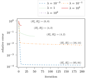
(a) Influence of $\lambda$ on BFB.

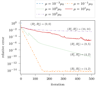
(b) Influence of $\mu$ on ALM.

Figure 2: Impact of the hyperparameters on the relative reconstruction error at each iteration on the multilinear transport test case. The co-moving ranks $R^{*}_{k}=\mathrm{rank}(\mathbf{Q}^{k})$ $k=1,2$ at iteration 500 are stated for each hyperparameter at the end of each line.

Performance evaluation. We compare the different algorithms with the following criteria: their computational efficiency (CPU time) along with the number of iterations before convergence, the ranks $R_{k}$ of the estimated co-moving fields $\{\mathbf{Q}^{k}\}_{k\in\llbracket 1,K\rrbracket}$, and the relative reconstruction error defined as $\left\lVert\mathbf{Q}-\sum_{k=1}^{K}\mathcal{T}^{k}(\mathbf{Q}^{k})-\mathbf{E}\right\rVert_{\mathrm{F}}/\left\lVert\mathbf{Q}\right\rVert_{\mathrm{F}}$. table 1 summarizes the performance comparison of the three proposed methods on the test cases described below.

Table 1: Performance comparison of the algorithms designed to solve Problem eq. 9 on our test cases. The lowest relative error and CPU times are highlighted in bold. $\mathcal{J}_{2}$ and $\mathcal{J}_{3}$ cannot estimate the ranks, the values indicated the input ranks. The cross means the original code cannot handle the data.

	JFB	BFB	ALM	$\mathcal{J}_{2}$	$\mathcal{J}_{3}$
	Relative error
Multilinear transport	1.88e-02	1.41e-02	1.9e-05	1.37e-03	6.4e-02
Sine waves	1.43e-02	7.96e-01	1.3e-04	1.45e-02	8.1e-01
Wildland fire (temperature)	9.1e-02	9.5e-02	2.1e-02	4.75e-02	$\times$
Two cylinders wake flow $u_{1}$	1.58e-03	1.58e-03	1.02e-02	8.43e-03	$\times$
Two cylinders wake flow $u_{2}$	1.1e-02	1.1e-02	1.62e-02	1.41e-02	$\times$
	Estimated ranks
Multilinear transport	(4,2)	(4,2)	(4,2)	(4,2)	(4,2)
Sine waves	(4,1)	(4,1)	(4,1)	(4,1)	(4,1)
Wildland fire (temperature)	(4,10)	(5,9)	(10,8)	(10,8)	$\times$
Two cylinders wake flow $u_{1}$	(203,228)	(209,221)	(40,31)	(40,31)	$\times$
Two cylinders wake flow $u_{2}$	(221,251)	(221,251)	(119,128)	(119,128)	$\times$
	CPU time
Multilinear transport	13s	16s	9s	28s	2s
Sine waves	75s	89s	14s	3s	1s
Wildland fire (temperature)	243s	331s	201s	70s	$\times$
Two cylinders wake flow $u_{1}$	12h	14h	34h	7h	$\times$
Two cylinders wake flow $u_{2}$	29h	29h	34h	7h	$\times$
	Number of iterations
Multilinear transport	162	174	104	500	1000
Sine waves	961	777	145	71	1000
Wildland fire (temperature)	15	18	7	6	$\times$
Two cylinders wake flow $u_{1}$	612	553	500	500	$\times$
Two cylinders wake flow $u_{2}$	1500	1500	500	500	$\times$

4.1 Validation on Synthetic data

We first test our algorithms on synthetic data for which the true decomposition of the snapshot matrix $\mathbf{Q}$ is known in order to validate numerically our approach.

4.1.1 Multilinear Transport

This example illustrates that, in a noiseless context, our algorithms are able to retrieve a low-rank decomposition with a low reconstruction error and the correct ranks. To this end, we generate a snapshot matrix $\mathbf{Q}$ of dimensions $400\times 200$ by discretizing the following transport-dominated field $q$ composed of two co-moving structures of ranks $(R_{1},R_{2})=(4,2)$

$$q(x,t)=\sum_{r=1}^{R_{1}}\sin(rt\pi)h(x+\Delta_{1}(t)-0.1r)+\sum_{r=1}^{R_{2}}\cos(rt\pi)h(x+\Delta_{2}(t)-0.1r)\,.$$

The initial spatial profile of the waves in each co-moving frame is given by $h(x)=\exp(-{x}^{2}/\delta^{2})$, with $\delta$ is set to $0.0125$ and the shift $(\Delta_{1},\Delta_{2})$ to $(t,-t)$. The discretization grid is obtained by uniformly discretizing the set $[-0.5,0.5]\times[0,0.5]$. Hence, after the shift transformations, the data fit on the grid and do not cause any interpolation error. Moreover, the data matrix $\mathbf{Q}$ is also free from any noise in the data. Consequently, $\mathbf{E}=\mathbf{0}$ in Model eq. 8.

We then apply the FB algorithms to decompose $\mathbf{Q}$ with $\lambda=0.3$ (for BFB), $\lambda=0.4$ (for JFB) and $\lambda_{K+1}=0$, as well as ALM with $\lambda=1$, $\lambda_{K+1}=0$ and $\mu=MN_{t}/(4||\mathbf{Q}||_{1})$. In fig. 3(a), we plot the relative error at each iteration of the algorithms while in fig. 4, we plot the evolution of the estimated co-moving ranks $(R^{*}_{1},R^{*}_{2})$. We first observe the descent property of FB methods, while ALM misses such a property. We then remark that all the methods retrieve the correct ranks. We also note that, although ALM reaches the maximum number of iterations, it has a better accuracy than the two FB methods. Moreover, table 1 shows that $\mathcal{J}_{2}$ reaches a machine precision relative error for the decomposition. However, in contrast with our proposed methods, $\mathcal{J}_{2}$ suffers from two drawbacks: (i) it requires to know explicitly the correct ranks, which is a challenging impediment on real data, (ii) it performs worse in the presence of noise as we will see in Section 4.1.2.

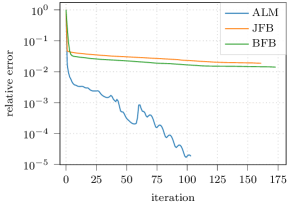
(a) Multilinear transport test case

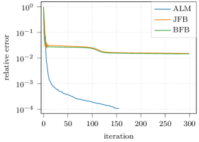
(b) Sine waves with noise test case.

Figure 3: Decay of the relative approximation error in the Frobenius norm.

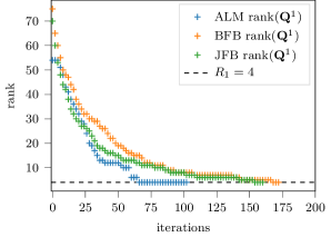
(a) Rank evolution of $\mathbf{Q}^{1}$.

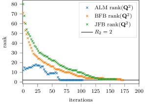
(b) Rank evolution of $\mathbf{Q}^{2}$.

Figure 4: Ranks of the estimated co-moving fields at each iteration for the multilinear transport test case.

4.1.2 Sine waves with noise

We now evaluate our methods in a noisy context. Similarly to the previous section, we generate a snapshot matrix $\mathbf{Q}$ with dimensions $400\times 200$ by discretizing the following field $q$ composed of two co-moving structures with ranks $(R_{1},R_{2})=(4,1)$

$$q(x,t)=\sum_{r=1}^{R_{1}}\sin(4\pi rt)h(x-0.1-025+\Delta_{1}(t))+h(x-0.2-\Delta_{2}(t))\,,$$

where $h(x)=\exp(-{x}^{2}/\delta^{2})$, $\delta=0.0125$, $(\Delta_{1},\Delta_{2})=(0.25\cos(7\pi t,-t)$, and the discretization grid is a uniform lattice on $[0,0.5]\times[0,1]$. In contrast to the previous example, the transformations $\mathcal{T}^{1}$ and $\mathcal{T}^{2}$ now introduce interpolation error to the data stored in $\mathbf{Q}$. Furthermore, we add a salt-and-pepper noise on the data $\mathbf{Q}$ by setting $12.5\%$ of its elements to $1$. The indices of the noised data are drawn randomly from a discrete uniform distribution. An illustration of the snapshot matrices and its sPOD decomposition was given in fig. 1.

We run our three algorithms with the parameters $\lambda=0.3$ and $\lambda_{K+1}=0.0135$ for FB methods and $\lambda=1$, $\lambda_{K+1}=1/\sqrt{\min(M,K)}$ and $\mu=\mu_{0}/10$ for ALM. Since $\mathcal{J}_{2}$ and $\mathcal{J}_{3}$ are not able to estimated the ranks for noisy data, we give them the correct ones to be able to conduct a comparison. Nonetheless, this is a severe restriction compared to our proximal methods. Figures 3(b) and 5 respectively show the relative error and the estimated ranks along the iterations. We observe that even in the presence of noise, our three methods estimate the correct ranks. Furthermore, ALM shows the lowest relative error as well as the lowest running time.

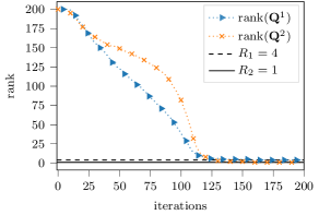
(a) BFB ($\lambda=0.3$, $\lambda_{K+1}=0.0135$).

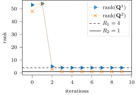
(b) ALM.

Figure 5: Ranks of the estimated co-moving fields at each iteration for the sine waves test case with noise.

4.2 2D Wildland-fire model

We now test our algorithms on the 2D wildland fire model given in [16] where authors use this model to assess the validity and the performance of their neural network-based sPOD. The model is composed of two coupled reaction-diffusion equations: one describing the evolution of the temperature with time, and the other one describing the evolution of the fuel supply mass fraction. We use similar model parameters as in [16] and showcase only the results with respect to the temperature, but similar statements hold when the supply mass fraction is included (see [16]). The differential equations are discretized using a $500\times 500$ equally spaced grid on the domain $[0,500]^{2}$ and integrated up to time $T_{\text{end}}=900$ for a reaction rate $\mu=558.49$ and wind velocity $v=0.2$. We then generate the snapshot matrix of the temperature with $100$ equally spaced snapshots.

A selected snapshot of the temperature profile is shown in fig. 6. In this simulation, a fire starts as an initial ignition with a Gaussian distribution in the center of the domain. Thereafter, a reaction wave spreads from the middle of the domain to the right, induced by a wind force. The ignition and traveling wave can be decomposed into a stationary frame and a frame that captures the traveling reaction wave.

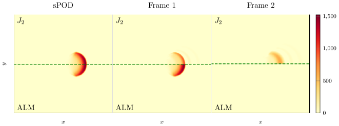
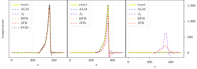
Figure 6: Decomposition results for the 2D wildland-fire test case with wind at $t=50$. The first row shows the sPOD approximation of the temperature and its decomposition in the individual frames using the $J_{2}$ (upper half) and ALM (lower half) algorithm. The second row shows a profile plot of all algorithms along the horizontal line at $y=250$ and the results of the POD with rank $R=18$. The ranks and approximation quality of all other algorithms are listed in table 1.

To separate the frames we set up the transforms as explained in [16] and run the different sPOD algorithms and validate their performance. We set $\lambda=2200$ and $\lambda_{K+1}=0$ for decomposing the temperature snapshot matrix using the FB algorithms. The results are visualized for one snapshot in fig. 6 and quantified in table 1. First, we observe that all sPOD algorithms approximate the data without the typical oscillatory effects induced by the POD (lower left profile picture). Furthermore, the direct comparison in fig. 6 shows that the $J_{2}$ algorithm is not able to separate the traveling reaction wave from the initial ignition impulse. In contrast, the proximal methods provide a better separation, whereas the ALM algorithm shows the best results. The noise part captured in $E$ is not shown in our examples as it only contains small interpolation errors.

4.3 Two cylinder wake flow

Lastly, we study the incompressible flow around two-cylinders simulated with the open source software WABBIT  [20]. The setup is visualized in fig. 7 and is inspired by biolocomotion, where the leader is followed by a chaser in a free-stream flow of uniform velocity $u_{\infty}$. In biolocomotion, the interaction between animals in close proximity, like fish or birds, are studied to understand their swarm behavior [67, 27]. In particular, one tries to explain swarm behavior with potential physics reasons, like energy minimization, or biological reasons, such as breeding or defense. To study a swarm from an idealist fluid dynamic perspective, a leading cylinder with a diameter $l$ is placed at a fixed position $(x_{1},y_{1})=(L/4,L/2)$ in a uniform flow at Reynolds number $\text{Re}=u_{\infty}l/\nu=200$ and the chaser further downstream $(x_{2},y_{2})=(L/2,L/2+\Delta_{\text{cyl}}(t))$ is shifted along a vertical path $\Delta_{\text{cyl}}(t)$ that is time-dependent. The vortex shedding generated by the first cylinder impacts the flow properties (drag and lift) of the second cylinder. To study the interactions between the two systems, they need to be separated, for example, using the proposed proximal algorithms.

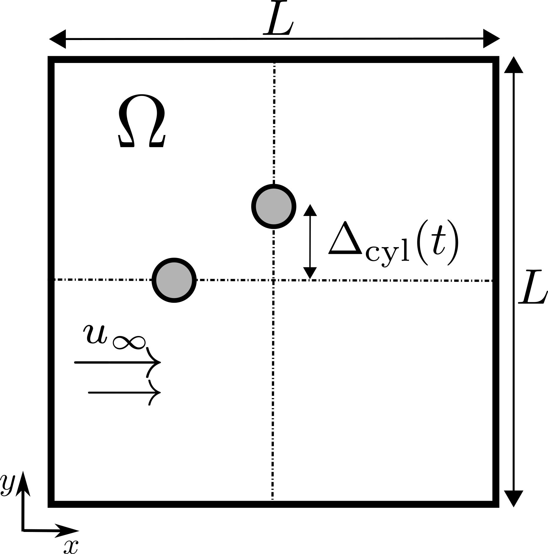
Figure 7: Illustration of the computational set-up of the two-cylinder simulation, one fixed, one vertically moving. The flow is driven by the inflow $u_{\infty}$, indicated by the arrows. Inside the computational domain $\Omega=[0,L]^{2}$, the flow passes the two cylinders, colored in gray, creating a vortex shedding. The fixed cylinder is located at $(x,y)=(L/4,L/2)$ and the moving cylinder at $(x_{2},y_{2})=(L/2,L/2+\Delta_{\mathrm{cyl}}(t))$.

The snapshot set for the example is built from the trajectory corresponding to the path $\Delta_{\text{cyl}}(t)=8.2\sin(2\pi f_{1}t)$ with $f_{1}=10f_{\mathrm{wake}}=0.2\times 10^{-2}s^{-1}$. Here, $f_{\mathrm{wake}}$ was calculated from the Strouhal number $\mathrm{St}=lf_{\mathrm{wake}}/u_{\infty}$ of the leading cylinder. The data are sampled with $\Delta t=1$ in time, resulting in $500$ snapshots. We sample a full period $T=500=1/f_{1}$ of the movement in an interval $[3T,4T]$. After the simulation, we upsample the adaptive grid to a uniform $512\times 512$ grid. All physical-relevant parameters like properties of the fluid are listed in table 2. Further information about the simulation can be found in [37].

Name	Value	Name	Value
Simulation time	$T_{\mathrm{end}}=2000$	Domain size	$[0,64]\times[0,64]$
Inflow velocity	$u_{\infty}=1$	Reynolds number	$\mathrm{Re}=200$
Cylinder diameter	$l=2$	Viscosity	$\nu=10^{-2}$

Table 2: Physical parameters of the two-cylinder simulation.

To reduce the data using the sPOD, we introduce the shift transformations. For the leading cylinder, a shift transformation is not needed since the cylinder is stationary ($\mathcal{T}^{1}=\operatorname{\mathrm{Id}}$). For the second one, we introduce the shift transform

$$\mathcal{T}^{2}(q)(x,y,t) =q(x,y+\Delta_{\text{cyl}}(t),t)\,,$$ (17)

that accounts for the movement of the cylinder and its vortex shedding.

With the imposed shifts, we apply the proximal algorithms separately to the individual velocity components $q=u_{1},u_{2}$ of the PDE solution. We apply the following strategies to compare the algorithms (i) we run the proximal algorithms until they reach the stopping critetion to obtain two co-moving fields $\{q^{k}\}_{k=1,2}$ with their corresponding truncation ranks $\{R_{k}^{*}\}_{k=1,2}$. (ii) We truncate the $\{q^{k}\}_{k=1,2}$ for all possible rank combinations $(R_{1},R_{2})\in\llbracket 1,R_{1}^{*}\rrbracket\times\llbracket 1,R_{2}^{*}\rrbracket$ and select the pairs $(R_{1},R_{2})$ for which the ROM with $R$ DOFs has the smallest truncation error. (iii) We run $\mathcal{J}_{2}$ algorithm on the exact same pairs $(R_{1},R_{2})$ determined from the previous step. The comparison of the resulting approximation errors for all algorithms can be seen in fig. 8. In the implementation of ALM, we set the parameters as follows: the initial value $\mu_{0}$ is defined as $MN_{t}/(4||\mathbf{Q}||_{1})$, $\mu$ is set to $5.0\times 10^{-3}\mu_{0}$, to $4.0\times 10^{-4}\mu_{0}$, and to $10^{-3}\mu_{0}$ for $u_{1}$, $u_{2}$, for $p$ respectively. For both ALM and FB, we configure the parameters with $\lambda=1$ and $\lambda_{K+1}=0$.

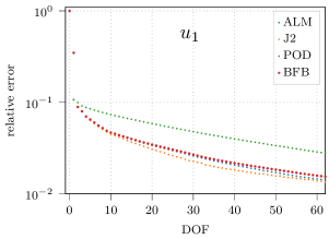
(a) Horizontal velocity component.

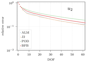
(b) Vertical velocity component.

Figure 8: Relative reconstruction error of the velocity fields $(u_{1},u_{2})$ in the Frobenius norm versus the DOFs. The DOFs are determined from the truncation rank $R$ of the POD and as the sum of the co-moving ranks $R=R_{1}+R_{2}$ in the case of $\mathcal{J}_{2}$ and the proximal algorithms, respectively.

As shown in fig. 8, the approximation errors are similar for all algorithms. The results of sPOD algorithms are superior to the results of the POD. Additionally, it should be pointed out that, in contrast to the proximal algorithms, $\mathcal{J}_{2}$ algorithm requires a separate run of the algorithm for every data point shown in fig. 8. Indeed, $\mathcal{J}_{2}$ optimizes ${q}^{1},{q}^{2}$ only for a fixed rank. However, this does not imply that the optimized co-moving fields have a fast singular value decay. As a consequence, $\mathcal{J}_{2}$ is not able to separate the two cylinders well. This is shown in fig. 9, which displays the two-dimensional vorticity field $\omega(x,y)=\partial_{x}u_{2}(x,y)-\partial_{y}u_{1}(x,y)$ resulting from the sPOD approximation of the velocity field $(u_{1},u_{2})$.

ALM

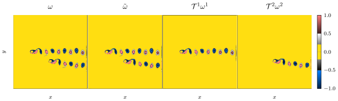
$\mathcal{J}_{2}$

Figure 9: Separation of the two moving cylinders. The vorticity field $\omega=\partial_{x}u_{2}-\partial_{y}u_{1}$ is displayed. It has been computed from the coupled cylinder pair and the reconstructed vorticity field $\tilde{\omega}=\omega^{1}+\omega^{2}$, with $\omega^{i}=\partial_{x}\mathcal{T}^{i}u_{2}^{i}-\partial_{y}\mathcal{T}^{i}u_{1}^{i}$, $i=1,2$. The co-moving ranks that are estimated by ALM and used as an input in $\mathcal{J}_{2}$ are $(R_{1},R_{2})=(40,31)$ for $(u_{1}^{1},u_{1}^{2})$ and $(R_{1},R_{2})=(119,128)$ for $(u_{2}^{1},u_{2}^{2})$. Separation similar to ALM is obtained with both FB algorithms (not shown here).

Besides the better approximation quality compared to the POD, we highlight the two important implications of this example, that could have been not achieved previously. (i) Since proximal algorithms are capable of separating the flow of the two systems, one can build a surrogate model for the individual systems that includes the path as a reduced variable. Therefore, it may be used to optimize the path of the second cylinder regarding drag or lift. (ii) The example allows to identify structures that can be attributed to the free-stream flow and structures that are responsible for the interaction. A first study in this direction can be found in [37].

5 Conclusion

We have presented three proximal algorithms for extending the sPOD for transport-dominated flows with multiple transports using a decomposition into co-moving linear subspaces. FB methods own enjoyable theoretical properties such as a descent lemma and convergence even in a non-convex setting like sPOD, whereas ALM demonstrates the best numerical results. Furthermore, we have shown that our methods can estimate the correct ranks of the different components of the sPOD. In contrast with the existing approaches, our methods are robust to noise. The numerical results show an accurate and strict separation of the involved transport phenomena. The close connection of our algorithms to the POD combined with the strict separation opens a new paradigm for flow optimization, control and analysis. A promising topic would consist in designing methods that can estimate both the co-moving structures and the associated transformation operators during the optimization stage.

Credit authorship contribution statement

In the following, we declare the authors’ contributions to this work.
P. Krah: Conceptualization, Methodology, Software, Writing – original draft. A. Marmin: Methodology, Formal Analysis, Software, Writing – original draft. B. Zorawski: Software, Visualization, Writing – review and editing. J. Reiss: Writing – review & editing, Funding acquisition. K. Schneider: Writing – review & editing, Funding acquisition, Project administration.

References

- [1] F. Arbes, C. Greif, and K. Urban, The Kolmogorov n-width for linear transport: Exact representation and the influence of the data. ArXiv Preprint, Apr. 2023, https://doi.org/10.48550/ARXIV.2305.00066, https://arxiv.org/abs/2305.00066.
- [2] H. Attouch, J. Bolte, and B. F. Svaiter, Convergence of descent methods for semi-algebraic and tame problems: proximal algorithms, forward–backward splitting, and regularized Gauss–Seidel methods, Math. Programm., 137 (2011), pp. 91–129, https://doi.org/10.1007/s10107-011-0484-9.
- [3] H. H. Bauschke and P. L. Combettes, Convex analysis and monotone operator theory in Hilbert spaces, in CMS Books in Mathematics, Springer New York, 2011, pp. 207–222, https://doi.org/10.1007/978-1-4419-9467-7_15.
- [4] A. Beck, First-order methods in optimization, Society for Industrial and Applied Mathematics, society for industrial & applied mathematics,u.s. ed., Oct. 2017, https://doi.org/10.1137/1.9781611974997.
- [5] P. Benner, S. Gugercin, and K. Willcox, A survey of projection-based model reduction methods for parametric dynamical systems, SIAM Rev., 57 (2015), pp. 483–531, https://doi.org/10.1137/130932715.
- [6] G. Berkooz, P. Holmes, and J. Lumley, The proper orthogonal decomposition in the analysis of turbulent flows, Annu. Rev. Fluid Mech., 25 (1993), pp. 539–575, https://doi.org/10.1146/annurev.fl.25.010193.002543.
- [7] F. Bernard, A. Iollo, and S. Riffaud, Reduced-order model for the BGK equation based on POD and optimal transport, J. Comput. Phys., 373 (2018), pp. 545–570, https://doi.org/10.1016/j.jcp.2018.07.001.
- [8] D. P. Bertsekas, Nonlinear programming, Athena Scientific, Belmont, Massachusetts, third edition ed., 2016.
- [9] F. Black, P. Schulze, and B. Unger, Projection-based model reduction with dynamically transformed modes, ESAIM Math. Model. Numer. Anal., 54 (2020), pp. 2011–2043, https://doi.org/10.1051/m2an/2020046.
- [10] F. Black, P. Schulze, and B. Unger, Efficient wildland fire simulation via nonlinear model order reduction, Fluids, 6 (2021), p. 280, https://doi.org/10.3390/fluids6080280.
- [11] F. Black, P. Schulze, and B. Unger, Modal decomposition of flow data via gradient-based transport optimization, Springer International Publishing, Nov. 2021, pp. 203–224, https://doi.org/10.1007/978-3-030-90727-3_13.
- [12] J. Bolte, A. Daniilidis, A. Lewis, and M. Shiota, Clarke subgradients of stratifiable functions, SIAM J. Optim., 18 (2007), pp. 556–572, https://doi.org/10.1137/060670080.
- [13] J. Bolte, S. Sabach, and M. Teboulle, Proximal alternating linearized minimization for nonconvex and nonsmooth problems, Math. Programm., 146 (2014), pp. 459–494, https://doi.org/10.1007/s10107-013-0701-9.
- [14] S. Boyd, Distributed optimization and statistical learning via the alternating direction method of multipliers, Found. Trends Mach. Learn., 3 (2010), pp. 1–122, https://doi.org/10.1561/2200000016.
- [15] S. Brivio, S. Fresca, N. R. Franco, and A. Manzoni, Error estimates for POD-DL-ROMs: a deep learning framework for reduced order modeling of nonlinear parametrized PDEs enhanced by proper orthogonal decomposition. ArXiv Preprint, May 2023, https://doi.org/10.48550/ARXIV.2305.04680, https://arxiv.org/abs/2305.04680.
- [16] S. Burela, P. Krah, and J. Reiss, Parametric model order reduction for a wildland fire model via the shifted pod based deep learning method. ArXiv Preprint, Apr. 2023, https://doi.org/10.48550/ARXIV.2304.14872, https://arxiv.org/abs/2304.14872.
- [17] E. J. Candès, X. Li, Y. Ma, and J. Wright, Robust principal component analysis?, J. ACM, 58 (2011), pp. 1–37, https://doi.org/10.1145/1970392.1970395.
- [18] E. Chouzenoux, J.-C. Pesquet, and A. Repetti, A block coordinate variable metric forward–backward algorithm, J. Global Optim., 66 (2016), pp. 457–485, https://doi.org/10.1007/s10898-016-0405-9.
- [19] P. L. Combettes and J.-C. Pesquet, Proximal splitting methods in signal processing, in Fixed-Point Algorithms for Inverse Problems in Science and Engineering, H. H. Bauschke, R. S. Burachik, P. L. Combettes, V. Elser, D. R. Luke, and H. Wolkowicz, eds., Springer, 2011, pp. 185–212.
- [20] T. Engels, K. Schneider, J. Reiss, and M. Farge, A wavelet-adaptive method for multiscale simulation of turbulent flows in flying insects, Commun. Comput. Phys., 30 (2021), pp. 1118–1149, https://doi.org/10.4208/cicp.oa-2020-0246.
- [21] F. Fedele, O. Abessi, and P. J. Roberts, Symmetry reduction of turbulent pipe flows, J. Fluid. Mech., 779 (2015), pp. 390–410, https://doi.org/10.1017/jfm.2015.423.
- [22] S. Fresca, L. Dedè, and A. Manzoni, A comprehensive deep learning-cased approach to reduced order modeling of nonlinear time-dependent parametrized PDEs, J. Sci. Comput., 87 (2021), https://doi.org/10.1007/s10915-021-01462-7.
- [23] S. Fresca and A. Manzoni, POD-DL-ROM: Enhancing deep learning-based reduced order models for nonlinear parametrized PDEs by proper orthogonal decomposition, Comput. Meth. Appl. Mech. Eng., 388 (2022), p. 114181, https://doi.org/10.1016/j.cma.2021.114181.
- [24] W. Gao, D. Goldfarb, and F. E. Curtis, ADMM for multiaffine constrained optimization, Optim. Methods Softw., 35 (2019), pp. 257–303, https://doi.org/10.1080/10556788.2019.1683553.
- [25] C. Greif and K. Urban, Decay of the Kolmogorov -width for wave problems, Applied Mathematics Letters, 96 (2019), pp. 216–222, https://doi.org/10.1016/j.aml.2019.05.013.
- [26] N. Halko, P. G. Martinsson, and J. A. Tropp, Finding structure with randomness: Probabilistic algorithms for constructing approximate matrix decompositions, SIAM Rev., 53 (2011), pp. 217–288, https://doi.org/10.1137/090771806.
- [27] C. K. Hemelrijk and H. Hildenbrandt, Schools of fish and flocks of birds: their shape and internal structure by self-organization, Interface Focus, 2 (2012), pp. 726–737, https://doi.org/10.1098/rsfs.2012.0025.
- [28] J. S. Hesthaven and S. Ubbiali, Non-intrusive reduced order modeling of nonlinear problems using neural networks, J. Comput. Phys., 363 (2018), pp. 55–78, https://doi.org/10.1016/j.jcp.2018.02.037.
- [29] C. Huang, K. Duraisamy, and C. Merkle, Challenges in reduced order modeling of reacting flows, in 2018 Joint Propulsion Conference, American Institute of Aeronautics and Astronautics, July 2018, https://doi.org/10.2514/6.2018-4675.
- [30] E. N. Karatzas, F. Ballarin, and G. Rozza, Projection-based reduced order models for a cut finite element method in parametrized domains, Comput. Math. Appl., 79 (2020), pp. 833–851, https://doi.org/10.1016/j.camwa.2019.08.003.
- [31] Y. Kim, Y. Choi, D. Widemann, and T. Zohdi, A fast and accurate physics-informed neural network reduced order model with shallow masked autoencoder, J. Comput. Phys., 451 (2022), p. 110841, https://doi.org/10.1016/j.jcp.2021.110841.
- [32] O. Koch and C. Lubich, Dynamical low‐rank approximation, SIAM J. Matrix Anal. Appl., 29 (2007), pp. 434–454, https://doi.org/10.1137/050639703.
- [33] J. Koellermeier, P. Krah, and J. Kusch, Macro-micro decomposition for consistent and conservative model order reduction of hyperbolic shallow water moment equations: A study using POD-Galerkin and dynamical low rank approximation. ArXiv Preprint, Feb. 2023, https://doi.org/10.48550/ARXIV.2302.01391, https://arxiv.org/abs/2302.01391.
- [34] J. Koellermeier, P. Krah, J. Reiss, and Z. Schellin, Model order reduction for the 1D Boltzmann-BGK equation: Identifying intrinsic variables using neural networks. ArXiv Preprint, Oct. 2023, https://doi.org/10.48550/ARXIV.2310.04318, https://arxiv.org/abs/2310.04318.
- [35] A. Kovárnová and M. Isoz, Model order reduction for particle-laden flows: Systems with rotations and discrete transport operators, in Topical Problems of Fluid Mechanics 2023, TPFM, Institute of Thermomechanics of the Czech Academy of Sciences; CTU in Prague Faculty of Mech. Engineering Dept. Tech. Mathematics, 2023, https://doi.org/10.14311/tpfm.2023.014.
- [36] A. Kovárnová, P. Krah, J. Reiss, and M. Isoz, Shifted proper orthogonal decomposition and artificial neural networks for time-continuous reduced order models of transport-dominated systems, in Topical Problems of Fluid Mechanics 2022, TPFM, Institute of Thermomechanics of the Czech Academy of Sciences, 2022, https://doi.org/10.14311/tpfm.2022.016.
- [37] P. Krah, Non-linear reduced order modeling for transport dominated fluid systems, phd thesis, Technische Universität Berlin, 2023, https://doi.org/10.14279/depositonce-16974.
- [38] P. Krah, S. Büchholz, M. Häringer, and J. Reiss, Front transport reduction for complex moving fronts: Nonlinear model reduction for an advection–reaction–diffusion equation with a Kolmogorov–Petrovsky–Piskunov reaction term, J. Sci. Comput., 96 (2023), https://doi.org/10.1007/s10915-023-02210-9.
- [39] P. Krah, T. Engels, K. Schneider, and J. Reiss, Wavelet adaptive proper orthogonal decomposition for large-scale flow data, Adv. Comput. Math., 48 (2022), https://doi.org/10.1007/s10444-021-09922-2.
- [40] P. Krah, M. Sroka, and J. Reiss, Model order reduction of combustion processes with complex front dynamics, Springer International Publishing, Aug. 2020, pp. 803–811, https://doi.org/10.1007/978-3-030-55874-1_79.
- [41] K. Kunisch and S. Volkwein, Galerkin proper orthogonal decomposition methods for a general equation in fluid dynamics, SIAM J. Numer. Anal., 40 (2002), pp. 492–515, https://doi.org/10.1137/s0036142900382612.
- [42] K. Kurdyka, On gradients of functions definable in o-minimal structures, Ann. de l’Institut Fourier, 48 (1998), pp. 769–783.
- [43] K. Lee and K. T. Carlberg, Model reduction of dynamical systems on nonlinear manifolds using deep convolutional autoencoders, J. Comput. Phys., 404 (2020), p. 108973, https://doi.org/10.1016/j.jcp.2019.108973.
- [44] Z. Lin, M. Chen, and Y. Ma, The augmented Lagrange multiplier method for exact recovery of corrupted low-rank matrices, J. Struct. Biol., 181 (2010), pp. 116–127, https://doi.org/10.1016/j.jsb.2012.10.010.
- [45] Z. Lin, R. Liu, and Z. Su, Linearized alternating direction method with adaptive penalty for low-rank representation, in Proc. Ann. Conf. Neur. Inform. Proc. Syst., J. Shawe-Taylor, R. Zemel, P. Bartlett, F. Pereira, and K. Weinberger, eds., vol. 24, Curran Associates, Inc., 2011, https://proceedings.neurips.cc/paper_files/paper/2011/file/18997733ec258a9fcaf239cc55d53363-Paper.pdf.
- [46] J. L. Lumley, The structure of inhomogeneous turbulence, A. M. Yaglom and V. I. Tatarski (Eds), Nauka, Moscow, 1967, pp. 166–178.
- [47] R. Mojgani and M. Balajewicz, Low-rank registration based manifolds for convection-dominated PDEs, Proceedings of the AAAI Conference on Artificial Intelligence, 35 (2021), pp. 399–407, https://doi.org/10.1609/aaai.v35i1.16116.
- [48] J.-J. Moreau, Proximité et dualité dans un espace hilbertien, Bull. Soc. Math. France, 93 (1965), pp. 273–299, http://eudml.org/doc/87067.
- [49] B. R. Noack, K. Afanasiev, M. Morziński, G. Tadmor, and F. Thiele, A hierarchy of low-dimensional models for the transient and post-transient cylinder wake, J. Fluid. Mech., 497 (2003), pp. 335–363, https://doi.org/10.1017/s0022112003006694.
- [50] M. Nonino, F. Ballarin, G. Rozza, and Y. Maday, Overcoming slowly decaying Kolmogorov n-width by transport maps: Application to model order reduction of fluid dynamics and fluid–structure interaction problems, Advances in Computational Science and Engineering, 1 (2019), pp. 36–58, https://doi.org/10.3934/acse.2023002, https://arxiv.org/abs/1911.06598.
- [51] K. Oberleithner, M. Sieber, C. Nayeri, C. O. Paschereit, C. Petz, H.-C. Hege, B. R. Noack, and I. Wygnanski, Three-dimensional coherent structures in a swirling jet undergoing vortex breakdown: stability analysis and empirical mode construction, J. Fluid. Mech., 679 (2011), pp. 383–414, https://doi.org/10.1017/jfm.2011.141.
- [52] M. Ohlberger and S. Rave, Reduced basis methods: Success, limitations and future challenges, in Proceedings of the Conference Algoritmy, 2016, pp. 1–12.
- [53] D. Papadimitriou and B. C. Vũ, An augmented Lagrangian method for nonconvex composite optimization problems with nonlinear constraints, Optim. Eng., (2023), https://doi.org/10.1007/s11081-023-09867-z.
- [54] B. Peherstorfer, Model reduction for transport-dominated problems via online adaptive bases and adaptive sampling, SIAM J. Sci. Comput., 42 (2020), pp. A2803–A2836, https://doi.org/10.1137/19m1257275.
- [55] B. Peherstorfer, Breaking the Kolmogorov barrier with nonlinear model reduction, Notices Amer. Mat. Soc., 69 (2022), p. 1, https://doi.org/10.1090/noti2475.
- [56] B. Peherstorfer and K. Willcox, Online adaptive model reduction for nonlinear systems via low-rank updates, SIAM J. Sci. Comput., 37 (2015), pp. A2123–A2150, https://doi.org/10.1137/140989169.
- [57] B. Recht, M. Fazel, and P. A. Parrilo, Guaranteed minimum-rank solutions of linear matrix equations via nuclear norm minimization, SIAM Rev., 52 (2010), pp. 471–501, https://doi.org/10.1137/070697835.
- [58] J. Reiss, Optimization-based modal decomposition for systems with multiple transports, SIAM J. Sci. Comput., 43 (2021), pp. A2079–A2101, https://doi.org/10.1137/20m1322005.
- [59] J. Reiss, P. Schulze, J. Sesterhenn, and V. Mehrmann, The shifted proper orthogonal decomposition: A mode decomposition for multiple transport phenomena, SIAM J. Sci. Comput., 40 (2018), pp. A1322–A1344, https://doi.org/10.1137/17m1140571.
- [60] D. Rim, B. Peherstorfer, and K. T. Mandli, Manifold approximations via transported subspaces: model reduction for transport-dominated problems, SIAM J. Sci. Comput., 45 (2023), pp. A170–A199, https://doi.org/10.1137/20m1316998.
- [61] R. T. Rockafellar, Convergence of augmented Lagrangian methods in extensions beyond nonlinear programming, Math. Programm., 199 (2022), pp. 375–420, https://doi.org/10.1007/s10107-022-01832-5.
- [62] C. W. Rowley, I. G. Kevrekidis, J. E. Marsden, and K. Lust, Reduction and reconstruction for self-similar dynamical systems, Nonlinearity, 16 (2003), pp. 1257–1275, https://doi.org/10.1088/0951-7715/16/4/304.
- [63] M. Salvador, L. Dedè, and A. Manzoni, Non intrusive reduced order modeling of parametrized PDEs by kernel POD and neural networks, Comput. Math. Appl., 104 (2021), pp. 1–13, https://doi.org/10.1016/j.camwa.2021.11.001.
- [64] L. Sirovich, Turbulence and the dynamics of coherent structures part I: Coherent structures, Q. Appl. Math., 45 (1987), pp. 561–571, https://www.jstor.org/stable/43637457.
- [65] T. Taddei and L. Zhang, Space-time registration-based model reduction of parameterized one-dimensional hyperbolic PDEs, ESAIM Math. Model. Numer. Anal., 55 (2021), pp. 99–130, https://doi.org/10.1051/m2an/2020073.
- [66] M. M. Valero, L. Jofre, and R. Torres, Multifidelity prediction in wildfire spread simulation: Modeling, uncertainty quantification and sensitivity analysis, Environmental Modelling & Software, 141 (2021), p. 105050, https://doi.org/10.1016/j.envsoft.2021.105050.
- [67] S. Verma, G. Novati, and P. Koumoutsakos, Efficient collective swimming by harnessing vortices through deep reinforcement learning, Proceedings of the National Academy of Sciences, 115 (2018), pp. 5849–5854, https://doi.org/10.1073/pnas.1800923115.
- [68] L. Vilar, S. Herrera, E. Tafur-García, M. Yebra, J. Martínez-Vega, P. Echavarría, and M. P. Martín, Modelling wildfire occurrence at regional scale from land use/cover and climate change scenarios, Environmental Modelling & Software, 145 (2021), p. 105200, https://doi.org/10.1016/j.envsoft.2021.105200.
- [69] Q. Wang, J. S. Hesthaven, and D. Ray, Non-intrusive reduced order modeling of unsteady flows using artificial neural networks with application to a combustion problem, J. Comput. Phys., 384 (2019), pp. 289–307, https://doi.org/10.1016/j.jcp.2019.01.031.
- [70] G. Welper, Transformed snapshot interpolation with high resolution transforms, SIAM J. Sci. Comput., 42 (2020), pp. A2037–A2061, https://doi.org/10.1137/19m126356x.