Experimental amplification and squeezing of a motional state of an optically levitated nanoparticle Martin Duchaň¹ , Martin Šiler¹  , Petr Jákl¹, Oto Brzobohatý¹, Andrey Rakhubovsky², Radim Filip², Pavel Zemánek¹ A contactless control of fluctuations of phase space variables of a nanoobject belongs among the key methods needed for ultra-precise nanotechnology and the upcoming quantum technology of macroscopic systems. Here we utilize the experimental platform of a single levitating nanoparticle (NP) to demonstrate essential protocols providing linear amplification of the mechanical phase space variables together with squeezing of phase space probability distribution. The protocol combines a controlled fast switching between the parabolic trapping potential and either weak parabolic or inverted parabolic amplifying potential leading to amplification of mean value and variance (fluctuations) along an arbitrary phase space variable and squeezing along the complementary one. The protocol is completed with cold damping scheme to control the initial fluctuations of the NP phase space variables. We reached the amplification gain $|G|>2$, the squeezing coefficient above 4 dB, and the second-order energy correlation function approaching 3 which corresponds to a maximum for a stochastic non-equilibrium classical state. These experimental results will already allow pre-amplification and manipulation of nanomechanical NP motion for all quantum protocols if the NP cooling towards the ground state is applied.  

1 Introduction

The recent experimental progress in the vacuum optical levitation of a single nanoparticle (NP) [1, 2, 3], more NPs [4, 5, 6, 7, 8, 9, 10], cooling of their translational and also rotational degrees of freedom down to the vicinity of the ground state of the quantum harmonic oscillator [11, 12, 13, 14, 15, 16] paves the way for the development of protocols that should test experimentally the quantum phenomena of such relatively large objects. Since the wavepacket at the ground state is spatially limited to a few pm, various methods are being proposed to enlarge it to overlap mechanical slits or to observe interference of the wave packet with itself in a potential of proper shape [17, 18, 19, 20, 21]. Considering, that the potential has to be changed fast and even radically change its profile, the experimental platform using optically levitated NP offers such a unique feature. The spatial profile of the trapping laser beam can be changed in a fraction of the period of the NP oscillation, minimizing also the gas and photon recoil heating, using acousto-optical deflectors or electro-optical modulators for oscillations up to hundreds of kHz [22, 23, 24, 16]. However, as we demonstrate below, proper timing of such potential switches offers amplifying coherent displacements of a mechanical oscillator with initial magnitudes even well below their zero-point fluctuations, similarly as by other methods [25, 26, 27, 28, 29, 30, 31].

However, such optomechanical amplification has much stronger applications to enhance both linear and nonlinear mechanical processes [32, 33, 34]. As state transfer and measurement have also limited efficiency, linear amplification of mechanical motion will be needed, similarly as in microwave [35] and optical experiments [36]. Moreover, such linear amplifiers of motion are essential elements in bosonic quantum technology protocols for manipulation and protection of quantum non-Gaussian states, as has been demonstrated in quantum optics [37, 38], trapped ions [39, 40] and superconducting circuits [41, 42].

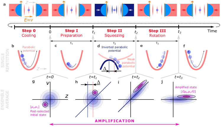
Figure 1: Illustration of the protocol of the optomechanical amplification (not to scale). a, Time sequence and geometry of the key steps. b, Initial levitation of the NP in a parabolic potential well formed by a standing optical wave (only $z$-motion is considered here). Cooling of the NP mechanical motion along the $z$-axis using an external electric field together with the cold damping feedback to the effective temperature $T_{\mathrm{0,CD}}$ at $t=0$. c, Time $0\leq t<t_{1}$, the preparation Step I of length $\tau_{1}$. The cooling is switched off at $t=0$, the recording of the NP position is on, and the NP moves in the parabolic potential with an angular frequency $\Omega_{c}$. d, Time $t_{1}\leq t<t_{2}$, the squeezing Step II of length $\tau_{2}$. The trapping parabolic potential is switched to a weak parabolic potential (WPP) and stronger inverted parabolic potential (IPP) is switched on (at $t=t_{1}$) but displaced by $\Delta$ from the WPP minimum. The NP moves down the potential hill in a sum of IPP (of characteristic angular frequency $\Omega_{i}$) and WPP ($\Omega_{w}$). e, Time $t_{2}\leq t\leq t_{3}$, the rotation Step III of length $\tau_{3}$. The WPP and IPP are switched off and the initial strong trapping parabolic potential is switched on at $t=t_{2}$. After a short transient system recovery ($\simeq 3\mu$s), the recording of NP positions is restored. The NP moves in the original harmonic potential ($\Omega_{c}$) and at time $t=t_{3}$, the final amplified state is reached. f, After $t>t_{3}$, the NP moves in the original parabolic potential and the protocol returns to Step 0 for the next repetition after a random delay which is illustrated with a dotted curve in a. For calibration purposes in each even repetition, we keep the parabolic potential unchanged (do not switch on WPP or IPP) and keep the recording on during Step II. g, Time $t=0$. The shaded area denotes the phase space probability density distribution (PSPD) of the NP occurrence as an ensemble average over many repetitions of Steps I-III at the time $t=0$ of each cycle. After the measurement, from the recorded trajectories sub-sets of initial states can be post-selected. One such initial state is denoted by pink shading and corresponds to the initial mean value $[\mu_{z},\mu_{v}]$, initial variances $\vartheta_{zz}$ and $\vartheta_{vv}$, and an initial effective temperature $T_{0}$ (see Methods). h, Time $t=t_{1}$. Due to the NP movement in the harmonic potential over $\tau_{1}$, the pre-selected PSPD rotated to the appropriate position for the subsequent amplification. i, Time $t=t_{2}$, the end of the amplification and squeezing of the pre-selected PSPD. j, Time $t=t_{3}$, the end of the whole amplification with the gain $G$. The pre-selected PSPD is rotated with its major semi-axis along the z axis, the amplified position is $G\mu_{z}$ and the variance of position increased $G^{2}\times$. In the case of negligible added noise, the final state mean velocity is $\mu_{v}/G$ and velocity fluctuations decreased $G^{2}\times$.

Here we demonstrate a promising experimental protocol that would enable the phase-sensitive amplification of the motional wavepacket and the accompanying phase space squeezing. Although it is demonstrated here with classical fluctuations, characterizing the probability density of a phase space state development is a well-established starting point to a quantum approach using the Wigner function representing general quantum state [43]. From the point of Hamiltonian mechanics, both in classical as well as quantum realms, the ideal phase-sensitive amplification represents the same linear canonical transformation for both classical and quantum observables of position and velocity (momentum). Since the phase space evolution of an experimental system can be viewed as a canonical transform as well, the tailored time-dependent changes of Hamiltonian would lead not only to a squeezing [44, 45, 46, 47], but to the expected phase-sensitive amplification. Moreover, the complementary phase space variable will become squeezed during the evolution of the system weakly interacting with the environment and keeping its phase space volume almost conserved by the Liouville theorem. In quantum mechanics, this turns to a fundamental preservation of commutation relations between position and momentum. Further, we demonstrate here the capability of the inverted parabolic potential to amplify the initial NP state, convert it to a position or velocity axis, squeeze its phase space fluctuations accordingly around its mean value, and characterize the level of added noise. Additionally, we confirm that the second-order energy correlation function approaches the upper stochastic limit equal to 3 for strongly amplified fluctuations [48], irrespective of initial noise.

A single loop of the repetitive protocol is illustrated and described in Fig. 1 as the modification of the experimental conditions leading to switching of the trapping parabolic and weak or inverted parabolic potentials (Fig. 1a). The parabolic potential well, spatially confining the levitating NP, is formed around the intensity maximum of the standing wave and its optical stiffness is controlled by the laser power. An NP levitates in a vacuum around a standing wave intensity maximum formed by two counter-propagating laser beams (along $z$-axis). For sufficiently small oscillations of the NP, the shape of the potential well can be considered parabolic (Fig. 1b). The magnitude of the NP oscillations can be further decreased using an external electric field combined with the cold damping feedback [49, 12, 8, 50, 5]. The level of such cooling can be characterized by an effective initial temperature $T_{0\mathrm{CD}}$ at $t=0$. At the moment, we are not able to reach experimentally as low temperatures as needed to approach states with variances close to the ground state or control them. Therefore, we took advantage of a large number of trajectories ($\approx 10^{5}$) acquired from the repeated protocol from Fig 1 and applied an ensemble averaging of trajectories. During such post-selection, we selected those trajectories fitting the desired properties of the initial state (Fig 1g, see Methods for details) and followed each of these experimental trajectories to time $t=t_{3}$, when their ensemble average defined the final state (Fig 1j). The experimental pre-cooling to $T_{0\mathrm{CD}}$ increases the density of trajectories if the post-selection requires initial states with very low variances. During the preparation Step I the pre-selected state is rotated in the phase space to a proper position for amplification or squeezing in Step II. Finally, it rotates during Step III with its major semiaxis to be parallel with the z or v axis for the amplification of position or velocity, respectively.

As we explain below, such a single-stage amplifier amplifies the NP mean position $G\times$ and the position variance $G^{2}\times$. However, Steps I-III (i.e. after the cooling and before the repetition of the protocol) can be repeated $N$ times with the same parameters after each other to obtain a multi-stage amplifier with the gain $G^{N}$ (if the reheating can be neglected). This way the larger amplification can be reached even if the single-stage gain is not sufficient.

2 Theoretical background

Being still in the classical stochastic regime, it is advantageous to work in dimensionless coordinates (denoted with a bar) where the normalization factor is given by the square root of the initial variance at $t=0$ of position/velocity of a NP in the parabolic potential well at an effective temperature $T_{0}$, i.e.

$$\bar{z} =\frac{z}{\sqrt{\vartheta_{zz}}}, \bar{v} =\frac{v}{\sqrt{\vartheta_{vv}}}, \bar{t} =\Omega_{c}t,$$ (1)

$$\vartheta_{zz} =\frac{k_{\mathrm{B}}T_{0}}{m\Omega_{c}^{2}}, \vartheta_{vv} =\frac{k_{\mathrm{B}}T_{0}}{m},$$ (2)

where $\vartheta_{zz}$ and $\vartheta_{vv}$ denote the initial state variances at $t=0$, $\Omega_{c}$ is the characteristic angular frequency of the harmonic oscillator corresponding to the parabolic potential (Steps 0, I, III), $k_{\mathrm{B}}$ the Boltzmann constant, and $m$ the NP mass.

If the sequence described above is so fast that the reheating can be ignored, the amplifier is ideal and does not add noise (i.e. the area of the phase space ellipse in Fig. 1g-j is constant). The action of an ideal amplifying protocol can be formally written as a linear transform (see the Supplementary Information (SI) for details) [51, 52]

$$\mathbf{\bar{z}}(t_{3})=\mathbf{R}_{3}\mathbf{P}\mathbf{R}_{1}\mathbf{\bar{z}}_{0}\equiv\mathbf{G}\mathbf{\bar{z}}(0)\equiv\left(\begin{array}[]{cc}G&0\\ 0&G^{-1}\end{array}\right)\left(\begin{array}[]{c}\bar{\mu}_{z}\\ \bar{\mu}_{v}\\ \end{array}\right)$$ (3)

where matrices $\mathbf{R}_{1}$ and $\mathbf{R}_{3}$ describe the rotation of the phase space probability distribution (PSPD) in the harmonic potential in Steps I and III. The matrix $\mathbf{P}$ describes the effect of the squeezing Step II. The initial and final phase space vectors are generally described as column vectors $\mathbf{\bar{z}}(0)=(\langle\bar{z}(0)\rangle,\langle\bar{v}(0)\rangle)^{T}\equiv(\bar{\mu}_{z},\bar{\mu}_{v})^{T}$ and $\mathbf{\bar{z}}(t_{3})=(\langle\bar{z}(t_{3})\rangle,\langle\bar{v}(t_{3})\rangle)^{T}$.

Considering the initial state that is normally distributed in the phase space with covariance matrix $\mathbf{\Theta}$, the covariance matrix at the final state $\mathbf{\Theta_{f}}$ at $t_{3}$ can be written as [53]

$$\mathbf{\Theta_{f}} = \mathbf{G\Theta G}^{T}.$$ (4)

In the ideal case of diagonal $\mathbf{G}$ matrix with reciprocal diagonal elements, the amplified noise variance would amplify/squeeze only the diagonal elements of the covariance matrix as

$$\mathbf{\Theta_{f}}=\left(\begin{array}[]{cc}\bar{\vartheta}_{zz}G^{2}&\bar{\vartheta}_{zv}\\ \bar{\vartheta}_{zv}&\bar{\vartheta}_{vv}G^{-2}\end{array}\right),$$ (5)

where $\bar{\vartheta}_{xx},\bar{\vartheta}_{vv},\bar{\vartheta}_{xv}$ denote the normalized elements of the covariance matrix $\mathbf{\Theta}$ at $t=0$.

The requirement for maximal amplification in a directly measurable position leads to zero off-diagonal terms of $\mathbf{G}$ and gives the following general analytical forms

$$G_{\pm} = \pm\mathcal{G}+\!(-1)^{k}\mathcal{A}\sqrt{1+\Psi^{2}},$$ (6)

$$\bar{\tau}_{1\pm} \equiv \Omega_{\mathrm{c}}\tau_{1}=\mp\frac{\pi}{4}-\frac{1}{2}\operatorname{atan}\Psi+k\frac{\pi}{2},$$ (7)

$$\bar{\tau}_{3\pm} \equiv \Omega_{\mathrm{c}}\tau_{3}=\pm\frac{\pi}{4}-\frac{1}{2}\operatorname{atan}\Psi+k\frac{\pi}{2}+\!2l\pi,$$ (8)

where $G_{\pm}$ is the gain for the particular solution $\pm$, $\bar{\tau}_{1}$ and $\bar{\tau}_{3}$ characterize the rotations $\mathbf{R}_{1}$ and $\mathbf{R}_{3}$ in Eq. (3), respectively. $k$ and $l$ denote independent integers, $\mathcal{G}$, $\mathcal{A}$, and $\Psi$ are expressed analytically in SI for all linear cases — i.e. the inverted parabolic potential (IPP), the parabolic potential of changed stiffness (e.g. WPP), free motion, or any combination of these three cases with additional external constant force. The factors $\mathcal{G}$, $\mathcal{A}$, and $\Psi$ are functions of $\bar{\tau}_{2}=\Omega_{c}\tau_{2}$ as well as the strength and direction of the acting force which may be characterized by a single parameter, angular frequency $\Omega_{i}$ for IPP or $\Omega_{w}$ for WPP.

It is worth stressing that the two solutions of $G_{\pm}$ for the same $k$ satisfy $G_{+}G_{-}=1$, i.e. if $|G_{+}|>1$ ($|G_{+}|<1$) the position (velocity) is amplified while the complementary coordinate is squeezed. Proper selection of even/odd $k$ and $\pm$ solutions determines if the amplifier operates in inverting or non-inverting mode, i.e. $G<0$ or $G>0$. Proper selection of $\tau_{1}$ and $\tau_{3}$ can minimize the length of the NP interaction with the optical parabolic potentials in Steps I and III and consequently can minimize the unwanted photon recoil heating (see details in SI). Moreover, in the IPP case, the potential maximum corresponds to the intensity minimum, and thus the photon recoil is minimal there.

In the case of non-zero IPP offset $\bar{\Delta}$ (Fig. 1d), an extra external optical force acts upon the NP, and the following term has to be added to Eq. (3):

$$\Delta\mathbf{\bar{z}}(t_{3})=\mathbf{R}_{3}\left(\begin{array}[]{c}\mathcal{A}-1\\ {\mathcal{G}}-\Psi\mathcal{A}\end{array}\right)\bar{\Delta}.$$ (9)

This, in analogy with the classical electronic, microwave or optical amplifier, enables us to select the amplifier operating point displaced from zero along a specific line in the phase space. Moreover, the offset $\bar{\Delta}$ does not influence the covariance properties.

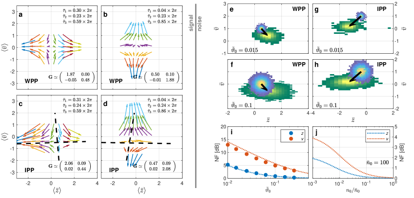
Figure 2: Performance of the optomechanical amplifier. a-d, Each arrow represents a displacement vector pointing from the initial selected position at $\bar{t}=0$ (arrow tail) to the final position measured at time $t_{3}$ of the amplification protocol (arrowhead). The values are determined as the mean values of 100 post-selected trajectories starting at the particular position (with ”zero” covariance). Text boxes provide the numerical values of all $\bar{\tau}_{1,2,3}$ giving depicted amplifier as well as elements of $\mathbf{G}$ matrix. (a, b) correspond to the position and velocity amplification, respectively, for different selections of $\bar{\tau}_{1}$ and $\bar{\tau}_{3}$ for the WPP case. Similarly, (c, d) show the same for the IPP. Due to the mismatch between the minimum of trapping and the maximum of inverted potentials, the center of the symmetry is shifted out of the linear part around the potential minimum and the distortion of the asymptotes (dashed curves) indicates such rising non-linearity. e-h, Experimental amplification from the initial noisy states (blue maps) to the final states (green maps) using the WPP (e, f) and IPP (g, h). The variances of the initial Gaussian PSPD were $\bar{\vartheta}_{xx}=\bar{\vartheta}_{vv}=\bar{\vartheta}_{0}=0.015$ (e, g) and $0.1$ (f, h). The black arrows follow the shift of the mean values of position and velocity. The $\mathbf{G}$ matrix and all $\bar{\tau}_{1,2,3}$ correspond to the data shown in panels a and c. i, Noise figure (NF) of the amplifier as a function of the input noise $\vartheta_{0}$ (points) and its estimated based on quantum mechanical computations (dotted) assuming initial thermal occupation number $n_{0}=1.5\times 10^{7}$ and the ambient pressure 1 mbar. j, Quantum mechanical simulation of NF corresponding to the evolution in WPP (a, only $\bar{\tau}_{2}$) as a function of initial thermal occupation ($\vartheta_{0}=2n_{0}+1$) assuming gas pressure reduced to $10^{-6}$ mbar and pre-cooling closer to the ground state $\bar{n}_{0}=100$ and $G_{\mathrm{z}}=1.87$. The experimental parameters are listed in Sec. LABEL:tab:expdata.

3 Experimental results

3.1 Amplification of initial mean values and noise

Using a levitated NP we recorded the sets of $1.6\times 10^{5}$ and $5\times 10^{5}$ trajectories for IPP and WPP potentials, respectively. Moreover, we interleaved each recorded trajectory (odd repetitions of the protocol in Fig. 1) by the same number of trajectories (even repetitions) with no change of the potential in Step II. The later ones were employed to determine the initial state variances of position and velocities and utilize them in the normalization of the experimental data following Eq. (1). It also enabled the characterization of the reheating rates during the thermalization of the system. The strength of IPP and WPP characterized by their corresponding relative angular frequencies is $\Omega_{i}/\Omega_{c}=0.41$, and $\Omega_{w}/\Omega_{c}=0.14$, respectively.

To determine the proper $\bar{\tau}_{1}$ and $\bar{\tau}_{3}$ giving ”zero” off-diagonal elements of the gain matrix $G_{zv}$ and $G_{vz}$ we considered different starting and ending times of the protocol (corresponding to different $\bar{\tau}_{1}$ and $\bar{\tau}_{3}$). For each combination of $\bar{\tau}_{1}$ and $\bar{\tau}_{3}$ we generated a set of $\sim$ 700 independent ensembles of trajectories (using the ”zero ” initial covariance post-selection, see Methods and SI), each originating in a different initial point $\mathbf{\bar{z}}_{0,i}$ in the phase space, and followed the trajectories to the final state $\mathbf{\bar{z}}_{f,i}$ corresponding to $\bar{\tau}_{3}$. Assuming linear transformation between the initial and final phase space positions we numerically determined the gain matrix elements. Finally, we took such selection of $\bar{\tau}_{1}$ and $\bar{\tau}_{3}$, which gave the minimal sum $|G_{zv}|+|G_{vz}|$. Using these values we obtained experimental gains of 1.87 and 2.06 for WPP and IPP, respectively. For details see SI.

Figure 2 summarizes the experimental amplification of the optomechanical state. Firstly, we demonstrate that by selection of the $\bar{\tau}_{1}$ and $\bar{\tau}_{3}$, the amplification of positions or velocities can be obtained for WPP (Fig. 2a-b) and IPP (Fig. 2c-d). This “classical” step should be done just once for the given potential and then applied for the quantum protocol where just a single event of position detection is allowed.

Taking the same measured dataset and $\bar{\tau}_{1}$ and $\bar{\tau}_{3}$ found in Fig. 2a,c, we applied the post-selection approach giving initial Gaussian distribution with variances $\bar{\vartheta}_{zz}=\bar{\vartheta}_{vv}=\bar{\vartheta}_{0}=0.015$ (Fig. 2e,g) and 0.1 (Fig. 2f,h) for WPP or IPP, respectively. The mean values are amplified by the same factor independent of the initial noise level as indicated by black arrows. Since the experimentally found off-diagonal elements of the gain matrix are small but non-zero, the amplified states (ellipses) are not perfectly oriented along the horizontal axis. The amplification and squeezing of the PSPD are visible for higher initial noise ($\bar{\vartheta}_{0}=0.1$) however, these effects are overshadowed by the strong reheating for low noise initial state ($\bar{\vartheta}_{0}=0.015$).

The added noise during the amplification can be characterized by the noise figure (see SI for details)

$$\mathrm{NF}^{(\xi)}=\frac{\mathrm{SNR}_{\mathrm{i}}^{(\xi)}}{\mathrm{SNR}_{\mathrm{o}}^{(\xi)}}=1+\frac{N_{\mathrm{a}}^{(\xi)}}{G_{\xi}^{2}\vartheta_{0}},$$ (10)

where $\xi=z$ ($\xi=v$) for the position (velocity), $\mathrm{SNR}_{\mathrm{i/o}}^{(\xi)}$ denotes the input and output signal-to-noise-ratio for position (velocity), and $G_{\mathrm{v}}=1/G_{\mathrm{z}}$. $N_{\mathrm{a}}^{(\xi)}$ denotes the noise added during the amplification to position (velocity), which corresponds to the thermal reheating and photon-recoil. To minimize $N_{a}$ and approach $\mathrm{NF}\simeq 1$ for low initial noise $\vartheta_{0}$ and fixed $G$, low ambient pressure and low light intensities incident on the NP are demanded.

NF for amplification of position or velocity is plotted in Fig. 2i for various levels of input noise. Since $G_{\mathrm{v}}\simeq 1/G_{\mathrm{z}}$, the velocity $\mathrm{NF}_{\mathrm{v}}$ is much larger than position $\mathrm{NF}_{\mathrm{z}}$ for a nonzero added noise $N_{\mathrm{a}}^{(\xi)}$. When the input noise level is above $\vartheta_{0}\geq 0.1$ the input signal-to-noise ratio (SNR_i) decreases, NF gets below 1 dB, and the output noise contains $\sim$ 20% of the noise generated internally in the amplification process. Quantum-theory-based simulations of the dynamics for the experimental parameters (dotted), including the photon recoil, support well the experimental observations. Figure 2j presents substantially smaller NF obtained from the simulations using quantum theory for various occupation numbers at lower pressure (where the photon recoil becomes dominant) and the mean occupation number closer to the ground state, compared to Figure 2i. The NFs obtained for the experimental geometry are comparable to those calculated for lower occupations which indicates the proposed approach applies to the future low-reheating quantum amplification.

3.2 Characterization of the extension and squeezing phase

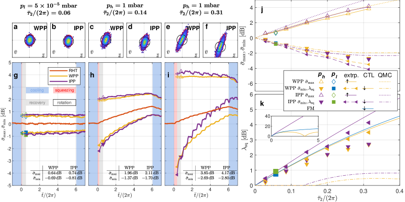
Figure 3: Evolution of a 2D phase space state after the squeezing phase. a-f, The PSPD after the squeezing for weak parabolic potential – WPP (a,c,e) and inverted parabolic potential – IPP (b,d,e) at the moment of signal recovery for low (a,b; $p_{l}$) and high (c-f; $p_{h}$) pressures and 3 different times $\bar{\tau}_{2}$. The PSPD time evolution for WPP and IPP of duration $\bar{\tau}_{2}/(2\pi)=0.31$ can be seen in the Supplementary Movie 1. The black circle and red ellipse correspond to the circle of radius 3 in the normalized coordinates done by the eigenvectors of the covariance matrix at the given time, respectively. g-i, The time evolution of the major semi-axis $\bar{\sigma}_{\mathrm{max}}$ and minor semi-axis $\bar{\sigma}_{\mathrm{min}}$ lengths in logarithmic scale obtained using the experimental data of the reference measurement (red - RHT), WPP (yellow), and IPP (purple). Thin parts of the curves in grey areas show the extrapolation of the state parameters obtained from fitting the data to the analytical forms of the covariance matrix for $\bar{t}<4\pi$ (SI Eqs. S116-S120, Fig. S12). The colors and markers used here have the same meaning as in panels j,k to stress the difference between the measured and extrapolated data. Tables at the bottom of each plot summarize the values of $\bar{\sigma}_{\mathrm{max}}$ and $\bar{\sigma}_{\mathrm{min}}$ at the times corresponding to the panels a-f. The evolution of additional parameters characterizing the state is plotted in SI Fig. S14. j, Comparison of the measured $\bar{\sigma}_{\mathrm{max}}$ and $\bar{\sigma}_{\mathrm{min}}$ (i.e. after the recovery of the detection denoted as the grey zone) obtained for various $\bar{\tau}_{2}$. Purple/yellow or blue/green colors of symbols correspond to the pressure 1 mbar or 5 $\times$ 10^-5 mbar, respectively. For comparison dotted and dash-dot curves denote the full quantum mechanics calculations (QMC) for IPP and WPP, respectively, in the presence of the photon recoil heating, at the level of experimental trapping power, initial occupation phonon number $n_{0}=0.5$, and gas pressure reduced to $1.4\times 10^{-6}$ mbar, at which the collisional and photon recoil heating rates are equal. k, Maximal squeezing coefficient $\lambda_{\mathrm{sq}}$ (Eq. (13)) as a function of the length $\bar{\tau}_{2}$ of the squeezing Step II. Yellow and purple dots depict the maximal measured values of $\lambda_{\mathrm{sq}}$ for WPP and IPP, respectively. The triangles show the extrapolated values of $\lambda_{\mathrm{sq}}$ to $\bar{t}=\bar{\tau}_{2}$, i.e. before the detection recovery when the squeezing phase ended. Blue and green squares show $\lambda_{\mathrm{sq}}$ for the low pressure. Blue, red, and yellow curves show the classical theoretical limits (CTL) for WPP, IPP, and free motion of given strength assuming zero reheating, see SI. The dot-dashed lines illustrate the results of the simulations of the squeezing in the quantum regime, for which $\bar{\sigma}_{\mathrm{min}}$ is normalized to the ground state spread (instead of the initial state). The inset shows the same theoretical limits of $\lambda_{\mathrm{sq}}$ for an extended time scale. The experimental parameters are listed in Sec. LABEL:tab:expdata.

Here we do not focus on the whole amplifier but only on the amplifying/squeezing Step II of length $\tau_{2}$ and the rotation Step III of an arbitrary length $\tau_{3}$ (assuming $\bar{\tau}_{1}=0$ in Fig. 1) because they are responsible for the level of amplification/squeezing and recording the subsequent amplified NP oscillations. Detailed analytical formulas for the state evolution at various levels of simplifications are expressed in the SI. The key effect of the squeezing phase is the change of the state covariance matrix which can be most naturally characterized by the lengths of the major $\bar{\sigma}_{\mathrm{max}}$ and minor $\bar{\sigma}_{\mathrm{min}}$ semi-axis of the Gaussian PSPD. A simplified and compact analytic formula for both semi-axes can be obtained for a very short Step II ($\bar{\tau}_{2}\ll 1$) assuming thermal initial state $\bar{\vartheta}_{zz}=\bar{\vartheta}_{vv}=\bar{\vartheta}_{0}$, and $\bar{\vartheta}_{zv}=0$ for free motion (FM), WPP, and IPP squeezing potentials:

$$\bar{\sigma}^{2}_{\begin{subarray}{c}\rm{max}\\ \rm{min}\end{subarray}}(\bar{\tau}_{2})=\bar{\vartheta}_{0}+\bar{\Gamma}\bar{\tau}_{2}\pm\kappa_{\rm{pot}}\bar{\vartheta}_{0}\bar{\tau}_{2}$$ (11)

where $\bar{\Gamma}=T\Gamma/(T_{0}\Omega_{c})$ is the damping coefficient in the normalized coordinates (Eq. (1)), $\kappa_{\rm{pot}}=1$ for FM, $\kappa_{\rm{pot}}=(1+\Omega_{i}/\Omega_{c})$ for IPP, and $\kappa_{\rm{pot}}=|1-\Omega_{w}/\Omega_{c}|$ for WPP. This simplified equation reveals that the IPP potential gives larger amplification/squeezing due to the larger $\kappa_{\rm{pot}}$ term if the characteristic frequencies for WPP and IPP are the same ($\Omega_{\mathrm{w}}=\Omega_{\mathrm{i}}$).

Immediately after Step II, the experimental system passes through a transient signal recovery ($\simeq 3\mu$s) before the detection of the NP position is possible. We aim to determine the elements of the covariance matrix $\bar{\vartheta}_{zz}(\bar{t}_{2})$, $\bar{\vartheta}_{vv}(\bar{t}_{2})$, $\bar{\vartheta}_{zv}(\bar{t}_{2})$ immediately after Step II (at $\bar{t}=\bar{t}_{2}$) from the experimental records of the NP position acquired during Step III. In the case of weak but non-negligible damping (see the SI for a more general case), the time dependence of $\bar{\sigma}_{\mathrm{max}}(\bar{\tau}_{3})$ and $\bar{\sigma}_{\mathrm{min}}(\bar{\tau}_{3})$ during Step III can be expressed:

$$\bar{\sigma}^{2}_{\begin{subarray}{c}\rm{max}\\ \rm{min}\end{subarray}}(\bar{\tau}_{3}) =\ \bar{\Gamma}\bar{\tau}_{3}+\frac{\bar{\vartheta}_{zz}\!+\!\bar{\vartheta}_{vv}}{2}\pm\frac{1}{2}\left\{\left(\bar{\vartheta}_{zz}\!-\!\bar{\vartheta}_{vv}\right)^{2}\!+\!4\bar{\vartheta}_{zv}^{2}\right.$$

$$\left.+4\bar{\Gamma}\left(\bar{\Gamma}\!\!-\!2\bar{\vartheta}_{zv}\right)\sin^{2}\bar{\tau}_{3}\!\!-\!2\bar{\Gamma}\left(\bar{\vartheta}_{zz}\!\!-\!\bar{\vartheta}_{vv}\right)\sin 2\bar{\tau}_{3}\right\}^{\frac{1}{2}},$$ (12)

where the first term $\bar{\Gamma}\bar{\tau}_{3}$ denotes the reheating factor. When no reheating is present (i.e. $\bar{\Gamma}=0$) the semi-axes are constant. However, in the presence of reheating and when the amplified covariance matrix is not diagonal or $\vartheta_{zz}(\bar{t}_{2})\neq\vartheta_{vv}(\bar{t}_{2})$, the lengths of the semi-axes oscillate in time.

Figures 3a-f show the two-dimensional PSPD obtained from experimental trajectories at ambient pressure 1 mbar and $5\times 10^{-5}$ mbar. Both amplification methods, WPP and IPP, show comparable amplification and squeezing at the same time. However, the shift of the mean value for the IPP is much larger due to the displacement of the potentials $\Delta\approx 73$ nm (see Methods). The amplification/squeezing at low pressure $5\times 10^{-5}$ mbar is much weaker because the experimental $\tau_{2}$ was about $4\times$ shorter to prevent the escape of the NP from the parabolic part of the optical trap.

Time evolution of the lengths of both semi-axes for low and high pressures (Figs 3g-i) reveal negligible reheating at low pressure (Figs 3g). Further, the IPP (purple) provides a slightly larger amplification which is fully revealed after extrapolation of the semi-axes lengths to $t=t_{2}$. Larger squeezing in longer Step II ($\bar{\tau}_{2}$) is accompanied by a faster thermalization of the minor semi-axes in Step III (compare Figs 3h and i) in contrast to the pure reheating (red RHT) during the calibration repetition. The reheating here, corresponding to $\vartheta_{0}=1$, causes only a weak increase of the noise level (see red curves) even at high pressure. However, there is no conflict with the NF results presented in Fig. 2i, because they were obtained by a post-selection from a colder initial state corresponding to the initial variances $0.01\leq\vartheta_{0}<0.25$. A comparison of experimentally obtained noise figures in Fig. 2i with the prediction for the quantum regime in Fig. 2j shows its substantial reduction achievable already by moderately lowering pressure to $10^{-6}$ mbar and cooling closer to the ground state.

Although a larger amplification, characterized by larger $\bar{\sigma}_{\mathrm{max}}$, is possible, it gets the state out of the linear regime of the optical trap and a Duffing-type non-linearity appears in such stochastic oscillator [54, 55, 56, 24].

Figure 3j compares the state amplification $\bar{\sigma}_{\mathrm{max}}$ with squeezing $\bar{\sigma}_{\mathrm{min}}$ for various $\bar{\tau}_{2}$ and WPP, IPP. While both values change reciprocally, the rates are not the same and can be described by excess noise $\delta$ (see SI). It conservatively estimates the thermalization contribution in the amplified phase-space variable separated from the noise corresponding to squeezed fluctuations in the ideal amplifier. The full quantum calculations were done analytically assuming the same stiffness of IPP and WPP, photon recoil heating at the experimental level, the ambient pressure reduced to $10^{-6}$ mbar, resulting in the same heating rate as the photon recoil level, and the initial occupation number $n_{0}=0.5$. As in the classical case, the ratios of the ellipse semi-axes to the initial variance (in the quantum case, $\bar{\sigma}_{0}^{2}=2n_{0}+1$) are presented. The increase of the length of the major semi-axis in time in the quantum case follows the classical case closely, indicating a similar amplification. The length of the minor semi-axis in the quantum regime does not follow the classical counterparts as closely, because the heating rates assumed in the simulations, expressed in the units of much smaller initial noise of the quantum regime, are higher than the heating rates of the classical experiment, expressed in units of the classical initial state. This illustrates the challenging character of reaching quantum squeezing that requires the suppression of $\bar{\sigma}_{\mathrm{min}}$ below the ground state spread.

The length of the minor semi-axis $\bar{\sigma}_{\mathrm{min}}$ is related to the squeezing and a squeezing coefficient $\lambda_{\mathrm{sq}}$ in units of dB [22] is introduced

$$\lambda_{\mathrm{sq}}=-10\log_{10}\bar{\sigma}_{\mathrm{min}}.$$ (13)

It is assumed here that the initial value is normalized to $\bar{\sigma}_{\mathrm{min}}=1$. Figure 3k compares $\lambda_{\mathrm{sq}}$ for different $\tau_{2}$ and WPP and IPP at the time of detection and extrapolated to the end of the squeezing period assuming the harmonic development of the NP during the transient detection recovery time after squeezing. The extrapolated experimental values (left pointing triangles) follow the theoretical limits (full curves) quite well with deviations caused by reheating appearing for longer $\bar{\tau}_{2}$. Due to frequent NP escape at low pressure, caused probably by the insufficient cooling in the transverse axes, only one squeezing time $\tau_{2}$ was investigated with the same NP. The inset shows $\lambda_{\mathrm{sq}}$ for longer times $\bar{\tau}_{2}$ and demonstrates the exponential rise of the IPP for longer $\bar{\tau}_{2}$ in contrast to linear increase or periodic behavior for free motion or WPP, respectively. The dot-dashed curves illustrate the squeezing calculated in the quantum regime, for which $\bar{\sigma}_{\mathrm{min}}$ is normalized to the ground state spread (instead of the initial state). Therefore, $\lambda_{\mathrm{sq}}>0$ indicates suppression of the mechanical fluctuations below the zero-point level [30, 57, 26]. The different normalization causes $\lambda_{\mathrm{sq}}(t^{\prime})=0$ for the initial times $t^{\prime}$ during which the minor noise semi-axis is already squeezed below the initial state, but not below the ground state yet. It can be seen, therefore, that reducing the pressure to $10^{-6}$ mbar and cooling the NP to mean occupations of approximately $n_{0}=0.5$ phonons, allows the generation of quantum sub-zero-point squeezing with the current experimental geometry.

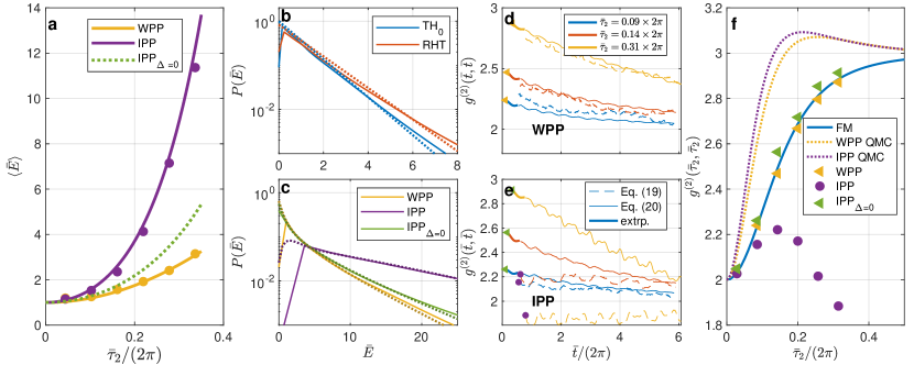
Figure 4: Energy gain, distribution, and second order coherence. a, Mean value of the NP energy as a function of the length $\bar{\tau}_{2}$ of the squeezing Step II for WPP (yellow points) and displaced IPP (purple points) from the experimental data using Eq. (15). The green dashed curve shows the IPP corrected for zero potential shift $\Delta=0$ using Eq. (17). The yellow, green and purple curves show the values obtained from Eqs. (S135, S137, and S141) without any fitting just using the known experimental parameters. b-c, PDF of the NP energy (solid curves) in states corresponding to the initial state (TH₀, last measured state prior switch to Step II), the reference measurement (RHT), WPP, IPP, and IPP_Δ=0 corrected for $\Delta=0$, all analyzed at $\bar{t}=\bar{\tau}_{2}+2\pi$, i.e. one period of state motion in Step III. Dotted curves for TH₀, RHT, WPP and IPP_Δ=0 show the results obtained from Eq. (18) using the values of $\bar{\sigma}_{\mathrm{max/min}}$ obtained in Sec. 3.2 or by the polar angle numerical integration of the displaced normal 2D PSPD (IPP). d-e, Evolution of the second order coherence $g^{(2)}(\bar{t},\bar{t})$ for WPP and IPP. Colors encode three different $\bar{\tau}_{2}$ enumerated in the label. Thin solid and dashed curves were obtained using covariance matrix elements using Eq. (20) and directly using Eq. (19), respectively. The thick solid curves at low $\bar{\tau}_{2}$ denote $g^{(2)}$ obtained from the elements of the covariance matrix extrapolated to this region (as in Fig. 3g-i). f, Values $g^{(2)}(\bar{t}_{2},\bar{t}_{2})$ extrapolated to $\bar{t}=\bar{t}_{2}$. The theoretical value for free motion given by Eq. (21), the blue curve, is compared to the WPP (yellow triangles) and IPP_Δ=0 (green triangles) obtained using Eq. (20) and to the IPP (purple dots) obtained using Eq. (19). For comparison yellow and purple dotted curves denote $g^{(2)}$ found using the full quantum mechanical calculations (QMC) for IPP and WPP overcoming the upper stochastic limit under the same conditions as in Fig. 3j. The experimental parameters are listed in Sec. LABEL:tab:expdata.

3.3 Energy characteristics

We aim to determine the increase of energy of the state during the squeezing phase via the detection of the NP position during Step III where the NP moves in the parabolic potential. Since the energy of the stochastic harmonic oscillator can be expressed as

$$\langle E\rangle =\frac{1}{2}m\Omega_{c}^{2}\langle z^{2}\rangle+\frac{1}{2}m\langle v^{2}\rangle\equiv\frac{1}{2}k_{B}T_{0}\left[\langle\bar{z}^{2}\rangle+\langle\bar{v}^{2}\rangle\right],$$ (14)

$$\langle\bar{E}\rangle \equiv\frac{1}{2}\left[\langle\bar{z}^{2}\rangle+\langle\bar{v}^{2}\rangle\right]=\frac{1}{2}\left[\langle\bar{z}\rangle^{2}+\langle\bar{v}\rangle^{2}+\bar{\theta}_{zz}+\bar{\theta}_{vv}\right],$$ (15)

where we employed the normal coordinates introduced in Eq. (1) and $T_{0}$ refers to the effective temperature at $t=0$ (done by initial variances via Eq. (2)) and $\bar{\theta}_{zz},\bar{\theta}_{vv}$ are variances of position/velocity at the given time. Assuming for simplicity the following condition during the squeezing phase $\bar{\tau}\,\Omega_{w/i}/\Omega_{c}\ll 1$ (see SI for full terms), one can get for the mean energy in the case of WPP and IPP with the same initial conditions:

$$\left\langle\bar{E}_{\begin{subarray}{c}\rm{WPP}\\ \rm{IPP}\end{subarray}}\right\rangle=\frac{1}{2}\left(1+\bar{\Gamma}\bar{\tau}\right)+\frac{1}{4}\bar{\tau}^{2}\left[1\mp\frac{\Omega_{w/i}^{2}}{\Omega_{c}^{2}}\right]^{2},$$ (16)

where $\Omega_{w/i}$ denotes the characteristic frequency corresponding to WPP or IPP, respectively. Considering the non-zero shift $\Delta$ of the IPP, the mean energy gains an extra term

$$\langle\bar{E}_{\rm{IPP}}^{(\bar{\Delta})}\rangle=\frac{1}{2}{\bar{\Delta}}^{2}{\bar{\tau}}^{2}\left(1+\frac{1}{4}\bar{\tau}^{2}\right).$$ (17)

Figure 4a shows the mean energy of the NP for various lengths of the squeezing period $\tau_{2}$ at pressure 1 mbar. The persuading effect of the strong energy increase due to the IPP is visible, even though the contribution from potential shifts $\bar{\Delta}$ (Eq. (17)) is subtracted (green dashed curve).

The probability density function (PDF) of the NP energy corresponding to a 2D Gaussian phase space state, having zero mean and covariance matrix $\bm{\Theta}$ in position and velocity, can be obtained by polar angle integration:

$$P(\bar{E})=\frac{1}{\bar{\sigma}_{\mathrm{max}}\bar{\sigma}_{\mathrm{min}}}\exp\left[-\frac{\bar{\sigma}_{2}^{(+)}\bar{E}}{2}\right]I_{0}\left(\frac{\bar{\sigma}_{2}^{(-)}\bar{E}}{2}\right)$$ (18)

where $\bar{\sigma}_{2}^{(\pm)}=|\bar{\sigma}_{\mathrm{min}}^{-2}\pm\bar{\sigma}_{\mathrm{max}}^{-2}|$ and $I_{0}$ is the modified Bessel function of the first kind and zero order. In the thermal state characterized by $\bar{\sigma}_{\mathrm{max}}=\bar{\sigma}_{\mathrm{min}}$ and Eq. (18) transforms to its standard exponential distribution. Bessel function, therefore, increases the probability of higher energy for moderate noise asymmetry $\bar{\sigma}_{2}^{(-)}$.

Figure 4b reveals that the PDF of the NP energy corresponds to the exponential distribution of the thermal state. In contrast, Fig. 4c demonstrates long-tail distribution typical for a system out-of-thermal state asymmetrical in the phase-space. A very good correspondence can be found between the experimental data (full) and the corresponding theoretical description by Eq. (18) (dotted) where the parameters $\bar{\sigma}_{\mathrm{min}},\,\bar{\sigma}_{\mathrm{max}}$ were taken from Sec. 3.2. Deviations for low $\bar{E}$ are not of physical origin but they are caused by the discretization and the features of the used PDF reconstruction algorithm.

The concept of the second-order coherence $g^{(2)}$, frequently used both in classical as well as in quantum optics, can be applied to the energy of the stochastic harmonic oscillator[58, 59, 60] $\bar{E}(t)=[\bar{z}(t)^{2}+\bar{v}(t)^{2}]/2$ at times $t$ and $t^{\prime}$:

$$g^{(2)}\left(t,t^{\prime}\right)=\frac{\left\langle\bar{E}(t)\bar{E}(t^{\prime})\right\rangle}{\left\langle\bar{E}(t)\right\rangle\left\langle\bar{E}(t^{\prime})\right\rangle}.$$ (19)

Since we investigate a non-stationary squeezed state coherence, we will focus on $g^{(2)}(\bar{t},\bar{t})$, i.e. with the zero lag coherence at the given time. Assuming the state with zero means, $g^{(2)}$ can be directly expressed using the elements of the covariance matrix $\bm{\Theta}$ as

$$g^{(2)}_{\mathrm{CM}}(\bar{t},\bar{t})=\frac{3\bar{\theta}_{zz}^{2}+2\bar{\theta}_{zz}\bar{\theta}_{vv}+3\bar{\theta}_{zz}^{2}+4\bar{\theta}_{zv}^{2}}{\bar{\theta}_{zz}^{2}+2\bar{\theta}_{zz}\bar{\theta}_{vv}+\bar{\theta}_{zz}^{2}}.$$ (20)

Figures 4d,e compare the time evolution of $g^{(2)}(\bar{t},\bar{t})$ during the rotation Step III for three different values of $\bar{\tau}_{2}$. Both approaches of $g^{(2)}(\bar{t},\bar{t})$ evaluation, using Eqs. (19 and 20), give comparable results for the WPP case and approach $g^{(2)}(\bar{t},\bar{t})=3$ for the longest $\bar{\tau}_{2}$. In contrast, both approaches give different results for the IPP. Since Eq. (20) assumed zero means, it corresponds to the case $\Delta=0$ because the nonzero $\Delta$ does not influence the covariance matrix. In contrast, Eq. (19) contains the mean values of the energy including also the contribution from nonzero $\Delta$. In this case, as $\bar{\tau}_{2}$ increases, $g^{(2)}(\bar{t},\bar{t})$ given by Eq. (19) decreases below 2 which indicates a more coherent state. The difference between the full and dashed curves in Fig. 4e thus expresses the influence of such nonzero $\Delta$ on $g^{(2)}(\bar{t},\bar{t})$.

Assuming an initial thermal-like state having the initial temperature $T_{0}$, i.e. $\bar{\vartheta}_{zz}=\bar{\vartheta}_{vv}=1$, $\bar{\vartheta}_{zv}=0$ and a negligible damping $\bar{\Gamma}$, one can find a simple relation for $g^{(2)}(\bar{\tau}_{2},\bar{\tau}_{2})$ in the simplest case of free motion (FM)

$$g^{(2)}_{\mathrm{FM}}(\bar{\tau}_{2},\bar{\tau}_{2})=\frac{8+12\bar{\tau}_{2}^{2}+3\bar{\tau}_{2}^{4}}{4+4\bar{\tau}_{2}^{2}+\bar{\tau}_{2}^{4}}.$$ (21)

At the time $\bar{\tau}_{2}=0$ one finds $g^{(2)}_{\mathrm{FM}}(0,0)=2$, which corresponds to the expected initial thermal state. However, at long times $\bar{\tau}_{2}\rightarrow\infty$, one receives for both FM as well as IPP

$$\lim_{\bar{\tau}_{2}\rightarrow\infty}g^{(2)}(\bar{\tau}_{2},\bar{\tau}_{2})=3.$$ (22)

Figure 4f reveals that experimental $g^{(2)}(\bar{\tau}_{2},\bar{\tau}_{2})$ for IPP_Δ=0 or WPP grows slightly faster or slower, respectively, than the theoretical value $g^{(2)}_{\mathrm{FM}}$ for free motion and all seem to converge to 3. The difference between them is not remarkable because also the squeezing coefficient in Fig. 3k does not change significantly. It complementary implies that the thermal state developed into the non-equilibrium mechanical state with an extended noise in a phase-space variable. In quantum optics such non-equilibrium fluctuations are used to activate nonlinear processes [61, 62] which could offer a similar advantage also for the optomechanical nonlinear processes. In contrast $g^{(2)}(\bar{\tau}_{2},\bar{\tau}_{2})$ for the IPP given by Eq.(19) and containing the nonzero potential shift $\Delta$ grows first above 2 but for longer times it decreases below 2. The energy of the state contains a significant contribution from the non-zero mean values which significantly enhances the denominator in Eq. (19) and decreases the second-order coherence of the state.

The full quantum calculations, repeated for the same conditions as in Fig. 3, give for certain $\bar{\tau}_{2}$, $g^{(2)}(\bar{\tau}_{2},\bar{\tau}_{2})>3$ for both IPP and WPP indicating a quantum phenomenon known from optics [63].

4 Conclusions and discussion

We present an experimental phase-sensitive amplification protocol, that uses an optically levitating NP interacting with up to two switchable standing waves. One experiment uses repetitive switching between the trapping parabolic potential, kept for a long time and formed near the standing wave antinode, and a weak parabolic potential (WPP), kept for a much shorter time $\tau_{2}$ in the same standing wave of lower power. The second approach adds the second standing wave approximately overlapping its nodes with the antinodes of the first standing wave and switched on shortly for $\tau_{2}$. Such an inverted parabolic potential (IPP) should provide stronger amplification of the phase space state of the NP, i.e. NP position or velocity. We characterize the properties of such optomechanical amplifier for ambient pressure 1 mbar, showing a noticeable added noise due to gas collisions, and $5\times 10^{-5}$mbar, with negligible collisional reheating. The latter one allowed only $\approx 4\times$ shorter amplification time $\tau_{2}$ to securely keep the NP in the parabolic part of the optical trap, however, this can be solved later involving an auxiliary Paul trap [64, 65]. Using both WPP and IPP we still reached the optomechanical gain $G\simeq 2$ for the mean values of position or velocity at $1$ mbar. The corresponding noise squeezing of $-1$ dB at low pressure and $-3$ dB at $1$ mbar was observed, too, with negligible reheating during the amplification compared to noise extension/squeezing.

The analysis of the probability density of the NP mechanical energy showed long-tail distributions corresponding to a strong deviation of the system from the thermal state. Evaluation of the second-order correlation function of the energy of the squeezed states approached the stochastic upper limit of $3$, indicating that the initial thermal state developed into a non-equilibrium mechanical state with an extended asymmetric noise in the phase-space variables [48].

Full quantum analyses were done for conditions close to the experimental ones to estimate how far is the experiment, run classically, from the quantum regime. Firstly we found, that the squeezing with the amplitude $\approx 1$ dB below the ground-state standard deviation is achievable at the current experimental level of the photon recoil heating [66] for the ambient pressure reduced to approximately $10^{-6}$ mbar and the NP initially cooled to the occupation of approximately $n_{0}=0.5$ phonons. Such experimental pressure and cooling level are reachable these days [11, 12, 13, 50, 15, 16, 67, 68].

Further reduction of the gas pressure to $10^{-8}$ mbar and, correspondingly, reduction of the collisional heating, would allow repetition of the amplification step of the presented protocol $N\times$ enabling the gain increase to $G^{N}$ with low added noise. Higher values of the gain allow the generation of quantum squeezing at much higher initial temperatures, e.g. $1$ dB of quantum squeezing is reachable starting from $n_{0}=10^{5}$ with $G^{N}\approx 6\times 10^{2}$.

Approaching quantum regime is also indicated by the quantum second-order correlation function $g^{(2)}>3$ (see [63]), i.e. over the classical stochastic limit. However, reaching this condition requires cooling to occupations $n_{0}\lesssim 1$ which is still doable at pressures below $10^{-6}$ mbar for the current experimental value of the photon recoil heating and the gain value $G\approx 2$.

The experiment proved the operation of a linear phase-sensitive amplifier in a stochastic but low-noise regime capable of extending/squeezing the mechanical motion. Such an extension or squeezing can be used before and after nonlinear dynamics provided by versatile trap potential, in order to intensify nonlinear effects and simplify their detection, which is necessary for fundamental tests and applications [1]. Moreover, we proved that such an experimental arrangement can be extended to the quantum regime using cooling methods. We leave extensive discussion of read-out and verification of the mechanical quantum states in such quantum experiments for subsequent analysis.

5 Methods

5.1 Experimental procedure

The experimental setup, data acquisition, and data processing are explained in more detail in the SI. In brief, we levitated silica NP (radius $a\approx 150$ nm) at pressures from 1 mbar down to $5\times 10^{-5}$ mbar in a standing wave formed from two counter-propagating laser beams of wavelength $1064$ nm. Each beam of power 20 mW passed through the high numerical aperture lens (NA = 0.77) and formed overlapping beam waists of radius $\approx 1\mu m$. In this study, we analyzed the axial motion of the NP that was detected in a balanced homodyne regime and obtained its mechanical oscillation frequency $\Omega_{0}/2\pi\approx 140$ kHz. The initial cooling of the NP motion was done by the cold damping [49, 12] with an electric field oriented along the z-axis.

The inverted parabolic potential is realized by the second beam of the same polarization but frequency-shifted. The potential profile was switched within $\approx 50$ ns by a simultaneous power decrease of each of the counter-propagating (CP) trapping beams to $\approx 2.5$ mW and an increase of the power in each of the second pair of counter-propagating beams to 8 mW using a pair of fiber acousto-optic modulators. The second beam is frequency shifted by $300$ MHz from the trapping beam and the optical path was designed in such a way that the intensity maxima of the second standing wave were displaced from the minima of the trapping standing wave by $\Delta\approx 73$ nm (see SI and Fig. 5). This way an inverted parabolic potential (IPP) profile is reached (Step II in Fig. 1). Similarly, if the trapping beam power is decreased as above but the second beam is not switched on, the weak parabolic potential (WPP) is generated for comparison. The original trapping potential (Step III in Fig. 1) is restored by an inverse switching process in both the IPP and WPP cases.

The measurement procedure started with the calibration phase when at least $10^{6}$ positions of the levitating NP were continuously recorded at a pressure of 1 mbar (without cooling) with a sampling rate of 9.76 MHz. Such a record was processed employing both positions and velocity power spectral density (PSD) functions [69]. This way the mechanical oscillation frequency $\Omega_{\mathrm{PSD}}/2\pi\approx 140$ kHz and the calibration factor 290 nm/V were determined and gave the standard position deviation of the levitating NP $\sqrt{\vartheta_{zz}}=11$ nm. Furthermore, using BEEPSIS [70] we verified our theoretical estimate that the acting optical force is linear in the extent of NP motion $\sim\pm 4\sqrt{\vartheta_{zz}}$ from the equilibrium position. Deviations greater than $\approx$ 70 nm from the equilibrium position were accompanied by a non-linear behavior. If required, the pressure in the vacuum chamber was consequently decreased, and the NP position was stabilized and cooled using the cold-damping feedback. The cooling was especially required to keep the particle trapped at the pressure $5\times 10^{-5}$ mbar. Afterward, another continuous record of NP positions might be taken to independently verify the initial state effective temperature $T_{\mathrm{0,CD}}$, that was determined from the change of the area below PSD curves compared to the previous room-temperature calibration measurement (see Fig. 6).

The calibration phase was followed by the stroboscopic sequence as described in Fig. 1. We varied the length of the amplification phase $\tau_{2}$ from 200 ns to 2.6 $\mu$s and recorded the position of the NPs in $-50\mu\mathrm{s}<t<0$ and $t_{2}+3\mu\mathrm{s}<t<40\mu\mathrm{s}$ to reconstruct the behavior of the NPs. The time delay of $3\mu$s corresponds to the transient recovery time for effects associated with the relaxation of the beam, NP, and detection electronics to the proper working conditions. The length of each cooling period (0.9 ms – 0.5 s, depending on pressure) is extended by a random amount in the range of 0 to 1 period to suppress the correlation with the previous state. The whole sequence was repeated $10^{4}-10^{6}\times$ to acquire the desired ensemble of trajectories. In each even repetition, the potential was not switched and the position recording was on for all the time $0\leq t\leq t_{3}$. This part served as the reference measurement of the NP behavior in unchanged the parabolic potential, to determine normalization factors, see Eqs. (2), and to study the purely reheating effects. Further details of the experimental procedure are given in SI.

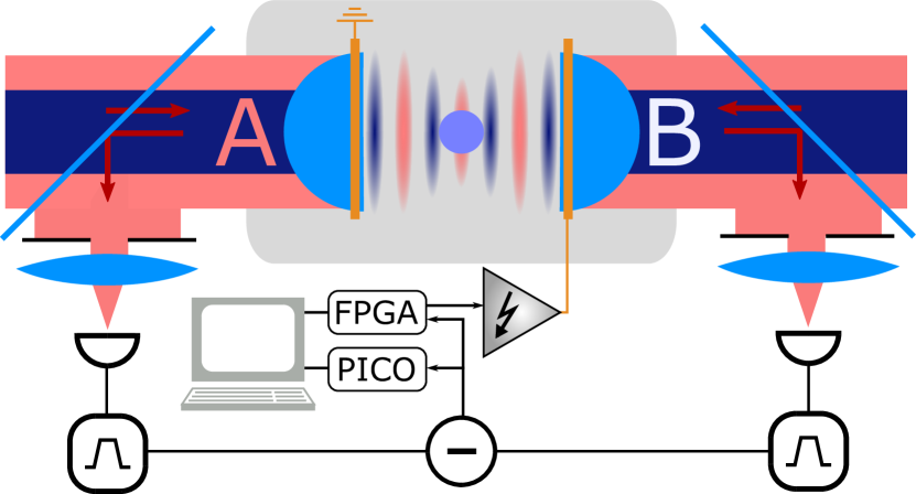
Figure 5: Switching geometry and cold damping. Two counter-propagating interfering beams form a standing wave and the NP levitates in its antinode (A). The second pair of counter-propagating beams (B) is switched on by an acoustic-optical modulator and due to its frequency shift of $300$ MHz for a standing wave with the nodes at the position of the antinodes of the beams A. Fast acoustic-optical switching between the beam A and B forms a parabolic trapping potential or inverted parabolic potential, respectively. Due to experimental imperfections, the nodes of beams B and antinodes of beams A are mismatched by about 70 nm. Cold damping is performed by electrodes placed at the rings of focusing lenses and via a feedback loop fed with a maximal voltage of 100 V. Two-sided balanced detection of NP axial motion. $\approx 10\%$ of the beam is reflected, spatially filtered, and focused on the photodiodes of the balanced detector. Signals are subtracted and filtered in the range of $100$ Hz$-$$100$ MHz. An additional $20\,$MHz low-pass antialiasing filter is used at the acquisition device (picoscope).

5.2 Detection

Position detection of the trapped NP is based on an optical homodyne method where the light scattered by the NP interferes at the detector with the unscattered trapping beam passing by the NP which serves as a local oscillator (see Fig. 5). The phase shift around the beam focus (Gouy phase shift) ensures that the mean phase of the scattered light is shifted by $\approx\pi/2$ at the detector from the phase of trapping light that passes through the focus. Further, the phase of the scattered light is modulated by the NP movement around its equilibrium position in the parabolic potential which leads to a linear response of the detected signal to the NP position around the equilibrium position ($z\ll\lambda$). Thanks to the geometry of the two counter-propagating trapping beams, we can detect scattered beam power from each beam by a pair of balanced photodiodes (Fig. 5), suppress the noise, and reach the linear detection.

$$\delta P(t)\simeq C_{0}+Cz(t)-[C_{0}-Cz(t)]=2Cz(t),$$ (23)

where $C_{0}$ is the intensity offset, $C$ is the detection efficiency and $z$ is the axial NP deviation from the equilibrium position. In the balanced regime, the intensity offset is subtracted and the full dynamic range of the detector and acquisition device is used for useful signal sampling which dramatically improves signal-to-noise ratio, see SI.

5.3 Cold damping

The cold damping feedback uses an external electric field between the electrodes mounted on the lens holders to create a feedback force $F_{\mathrm{fb}}=-\gamma[z(t)-z(t-\delta t)]f_{\rm{fb}}$ acting upon the naturally triboelectrically charged levitated NP, where the feedback sampling frequency $f_{\rm{fb}}=1/\delta t$. Figure 6 compares the power spectral densities of the NP positions for room temperature and with cold damping feedback.

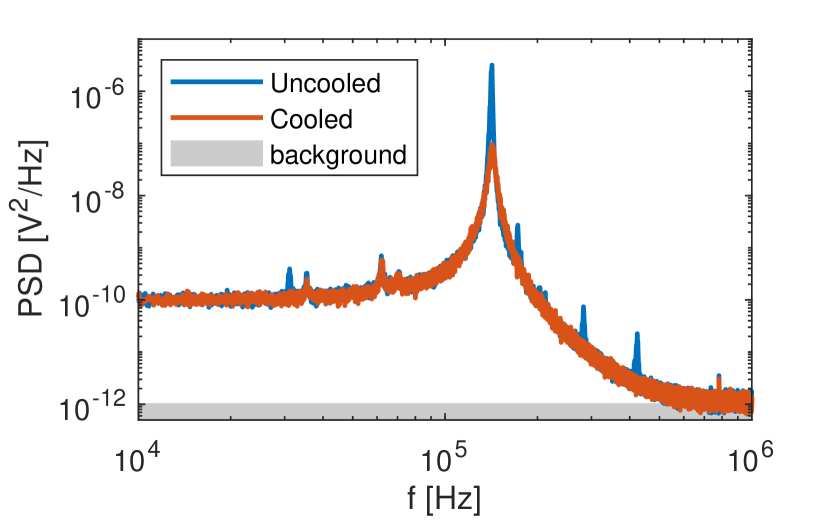
Figure 6: Power spectral densities of NP position for room temperature (blue) and with cold damping feedback active (red) at 1 mbar. The dominant oscillation frequency is 140 kHz and its peak decreases by approximately 2 orders of magnitude as the result of the cold damping feedback.

5.4 Parameters of the experiments

The experimental parameters for particular measurements presented in corresponding figures are summarized below.

Arrangement	Amplifier	Squeezing/	Squeezing
		Energy
Figure	Fig. 2	Figs. 3,4,6	Fig. 3
$p$ [mBar]	1	1	$5\times 10^{-5}$
$\tau_{2}$ [ns]	1 800	200 - 2 200	400
$\sqrt{\vartheta_{zz}}$ [nm]	14.8	11.0	4.0
$T_{\mathrm{0,CD}}$ [K]	300	198	27
$\Omega_{c}/2\pi$ [kHz]	130WPP	143.9	140.7
	131.5IPP
$\Omega_{i}/\Omega_{c}$	0.41	0.41	0.41
$\Omega_{w}/\Omega_{c}$	0.14	0.14	0.14
Trajectories	500 000 WPP	5 000	5 000
	165 000 IPP

5.5 Data post-selection

When working with large data ensembles (in our case up to $5\times 10^{5}$) of repeated experimental realizations of the same physical process, one may, in principle, select a certain data sub-set that satisfies a given set of constraints that are difficult to reach experimentally (e.g. the initial position or variance). Let us refer to such a procedure as the post-selection. We aim to select a sub-set of recorded trajectories, that in a given (initial) time lead to a prescribed state characterized by means and covariance matrix. We developed different procedures to select a data sub-set with “zero” initial covariance or with a given prescribed initial Gaussian distribution. However, as the recorded dataset is not infinite, we are not able to obtain the prescribed states exactly, moreover, the post-selected phase space probability distribution may not be Gaussian and may contain non-Gaussian higher moments.

“Zero” initial covariance: The prescribed sub-set should lead to mean position $\bar{\mu}_{zp}$ and mean velocity $\bar{\mu}_{vp}$ with as small variance and covariance as possible. However, the exact values of the covariance matrix are not important and the distribution of initial points could deviate from Gaussian.

The trajectory sub-set is selected using the following procedure:

1. In normal phase space coordinates an Euclidean distance between prescribed mean values and experimentally measured positions (at initial time) is calculated.

2. Up to $N$ points closest to the prescribed position is taken into sub-set. Alternatively, all points within the given radius are included in the sub-set.

Prescribed initial Gaussian distribution: The initial probability distribution of the post-selected data should follow the Gaussian distribution

$$P_{p}=\frac{1}{2\pi\sqrt{\det\mathbf{\bar{\Theta}_{p}}}}\exp\left\{-\frac{1}{2}(\bm{\bar{z}}-\bm{\bar{\mu}_{p}})^{T}\mathbf{\bar{\Theta}_{p}}^{-1}(\bm{\bar{z}}-\bm{\bar{\mu}_{p}})\right\},$$ (24)

where $\mathbf{\bar{\Theta}_{p}}$ is the prescribed covariance matrix; $\bm{\bar{z}}=(\bar{z},\bar{v})^{T}$, and $\bm{\bar{\mu}_{p}}=(\bar{\mu}_{zp},\bar{\mu}_{vp})^{T}$ are the column vectors of phase-space positions and prescribed initial position, respectively.

To create an ensemble of post-selected trajectories with initial condition fulfilling Eq. (24) we developed an approach based on a “survivor function,” i.e. for each trajectory a probability $P_{s}$ that the trajectory falls into the post-selected ensemble is defined. The procedure of trajectory post-selection is following (and demonstrated using a random 1D sample shown in Fig. 7a):

1. Reconstruction of the phase space probability density function (PDF) of the whole ensemble $P_{0}$ (red curve in Fig. 7b). It may differ from the ideal underlying PDF (blue curve). If the number of trajectories is reasonably high, simple histograms may be used, otherwise, a kernel smoothing approach is recommended.

2. Renormalization of $P_{0}$ in the following way

   $$P_{0n}=\min\left[1,P_{0}(\bm{\bar{z}})/P_{0}(\bm{\bar{\mu}_{p}})\right],$$ (25)

   i.e. it equals to 1 in the maximum of the prescribed PDF and is coerced to interval 0–1.

3. Calculation of a “survivor” probability for each trajectory if it belongs to a post-selected ensemble (i.e. phase space position in initial time):

   $$P_{s}(\bm{\bar{z}})=P_{p}(\bm{\bar{z}})/P_{0n}(\bm{\bar{z}}).$$ (26)

   Examples of prescribed PDF and survivor probability are depicted in Fig. 7c-d, respectively.

4. Generation of a uniformly distributed random number $r$ in the range 0–1. If $r<P_{s}(\bm{\bar{z}})$ the given trajectory will be taken as part of the post-selected ensemble. Figure 7e shows such a “post-selected” ensemble consisting of 69 points.

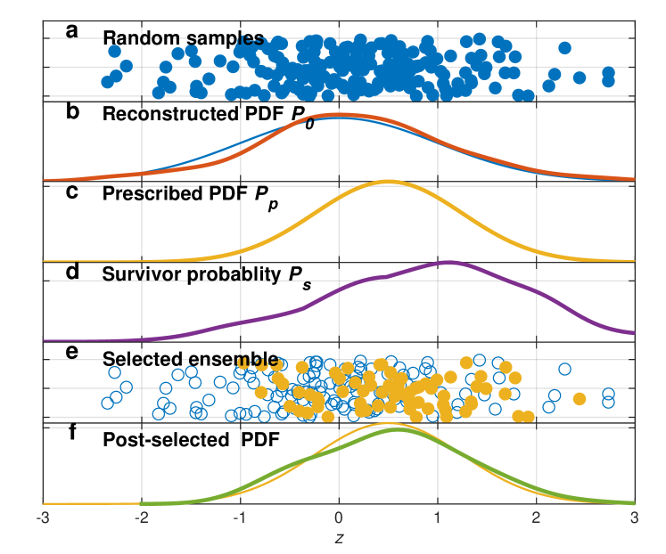
Figure 7: Principle of data post-selection for generation of a given probability density function (PDF). For details see text.

Finally, Fig. 7f compares the PDF generated by the post-selection process (green curve) to the prescribed PDF (yellow curve). However, due to the limited data sample the resulting PDF also contains higher non-Gaussian moments, e.g. skewness of 0.1 and kurtosis of 2.6.

This rather simple approach will introduce bias and discrepancy between prescribed $P_{p}$ and actually “measured by post-selection” data. Therefore, one should always take into account real values of means and covariance matrix for a given post-selected ensemble instead of prescribed values. Also, we should keep in mind that as the selection is based on the random process repeated post-selection will lead to different post-selected ensemble realizations.

Contributions

PZ and RF managed the project, developed the basic idea and its experimental realization, and analyzed some of the results. MD and OB designed the experimental setup, PJ developed the synchronized control of the experiment and data acquisition, MD built the experiment and performed all the measurements, MS analyzed the experimental and theoretical data, developed the stochastic theory, AR and RF performed the simulations and analysis of the quantum regime. All authors contributed to the preparation of the manuscript.

References

- [1] Gonzalez-Ballestero, C., Aspelmeyer, M., Novotny, L., Quidant, R. & Romero-Isart, O. Levitodynamics: Levitation and control of microscopic objects in vacuum. Science 374, eabg3027 (2021). URL https://www.science.org/doi/10.1126/science.abg3027. Publisher: American Association for the Advancement of Science.
- [2] Millen, J., Monteiro, T. S., Pettit, R. & Vamivakas, A. N. Optomechanics with levitated particles. Reports on Progress in Physics 83, 026401 (2020). URL https://dx.doi.org/10.1088/1361-6633/ab6100. Publisher: IOP Publishing.
- [3] Winstone, G. et al. Levitated optomechanics: A tutorial and perspective (2023). URL http://arxiv.org/abs/2307.11858. ArXiv:2307.11858 [physics, physics:quant-ph].
- [4] Rieser, J. et al. Tunable light-induced dipole-dipole interaction between optically levitated nanoparticles. Science 377, 987–990 (2022). URL https://www.science.org/doi/10.1126/science.abp9941. Publisher: American Association for the Advancement of Science.
- [5] Liška, V. et al. Cold damping of levitated optically coupled nanoparticles. Optica 10, 1203 (2023). URL https://opg.optica.org/abstract.cfm?URI=optica-10-9-1203.
- [6] Liška, V. et al. Observations of a PT-like phase transition and limit cycle oscillations in non-reciprocally coupled optomechanical oscillators levitated in vacuum (2023). URL https://arxiv.org/abs/2310.03701.
- [7] Reisenbauer, M. et al. Non-Hermitian dynamics and nonreciprocity of optically coupled nanoparticles (2023). URL http://arxiv.org/abs/2310.02610. ArXiv:2310.02610 [cond-mat, physics:physics, physics:quant-ph].
- [8] Vijayan, J. et al. Scalable all-optical cold damping of levitated nanoparticles. Nature Nanotechnology 1–6 (2022). URL https://www.nature.com/articles/s41565-022-01254-6. Publisher: Nature Publishing Group.
- [9] Arita, Y. et al. All-optical sub-Kelvin sympathetic cooling of a levitated microsphere in vacuum. Optica 9, 1000–1002 (2022). URL https://opg.optica.org/optica/abstract.cfm?uri=optica-9-9-1000. Publisher: Optica Publishing Group.
- [10] Arita, Y., Wright, E. M. & Dholakia, K. Optical binding of two cooled micro-gyroscopes levitated in vacuum. Optica 5, 910–917 (2018). Publisher: OSA.
- [11] Delić, U. et al. Cooling of a levitated nanoparticle to the motional quantum ground state. Science 367, 892–895 (2020).
- [12] Magrini, L. et al. Real-time optimal quantum control of mechanical motion at room temperature. Nature 595, 373–377 (2021). URL https://www.nature.com/articles/s41586-021-03602-3. Publisher: Nature Publishing Group.
- [13] Tebbenjohanns, F., Mattana, M. L., Rossi, M., Frimmer, M. & Novotny, L. Quantum control of a nanoparticle optically levitated in cryogenic free space. Nature 595, 378–382 (2021). URL https://www.nature.com/articles/s41586-021-03617-w.
- [14] Kamba, M., Shimizu, R. & Aikawa, K. Nanoscale feedback control of six degrees of freedom of a near-sphere. Nature Communications 14, 7943 (2023). URL https://www.nature.com/articles/s41467-023-43745-7. Publisher: Nature Publishing Group.
- [15] Arita, Y. et al. Cooling the optical-spin driven limit cycle oscillations of a levitated gyroscope (2022). URL http://arxiv.org/abs/2204.06925. ArXiv:2204.06925 [physics].
- [16] Kamba, M. & Aikawa, K. Revealing the velocity uncertainties of a levitated particle in the quantum ground state (2023). URL http://arxiv.org/abs/2306.16598. ArXiv:2306.16598 [physics, physics:quant-ph].
- [17] Neumeier, L., Ciampini, M. A., Romero-Isart, O., Aspelmeyer, M. & Kiesel, N. Fast Quantum Interference of a Nanoparticle via Optical Potential Control. Proceedings of the National Academy of Sciences 121, e2306953121 (2024). URL http://arxiv.org/abs/2207.12539. ArXiv:2207.12539 [cond-mat, physics:quant-ph].
- [18] Roda-Llordes, M., Riera-Campeny, A., Candoli, D., Grochowski, P. T. & Romero-Isart, O. Macroscopic Quantum Superpositions via Dynamics in a Wide Double-Well Potential. Physical Review Letters 132, 023601 (2024). URL http://arxiv.org/abs/2303.07959. ArXiv:2303.07959 [cond-mat, physics:quant-ph].
- [19] Wu, Q., Ciampini, M. A., Paternostro, M. & Carlesso, M. Quantifying protocol efficiency: A thermodynamic figure of merit for classical and quantum state-transfer protocols. Physical Review Research 5, 023117 (2023). URL https://link.aps.org/doi/10.1103/PhysRevResearch.5.023117. Publisher: American Physical Society.
- [20] Rakhubovsky, A. A. & Filip, R. Stroboscopic high-order nonlinearity for quantum optomechanics. npj Quantum Information 7, 1–7 (2021). URL https://www.nature.com/articles/s41534-021-00453-8. Publisher: Nature Publishing Group.
- [21] Weiss, T., Roda-Llordes, M., Torrontegui, E., Aspelmeyer, M. & Romero-Isart, O. Large Quantum Delocalization of a Levitated Nanoparticle Using Optimal Control: Applications for Force Sensing and Entangling via Weak Forces. Physical Review Letters 127, 023601 (2021). URL https://link.aps.org/doi/10.1103/PhysRevLett.127.023601. Publisher: American Physical Society.
- [22] Rashid, M. et al. Experimental Realization of a Thermal Squeezed State of Levitated Optomechanics. Physical Review Letters 117, 273601 (2016). URL https://link.aps.org/doi/10.1103/PhysRevLett.117.273601.
- [23] Hebestreit, E., Frimmer, M., Reimann, R. & Novotny, L. Sensing Static Forces with Free-Falling Nanoparticles. Physical Review Letters 121, 063602 (2018). URL https://link.aps.org/doi/10.1103/PhysRevLett.121.063602. Publisher: American Physical Society.
- [24] Muffato, R. et al. Generation of classical non-Gaussian distributions by squeezing a thermal state into non-linear motion of levitated optomechanics (2024). URL http://arxiv.org/abs/2401.04066. ArXiv:2401.04066 [quant-ph].
- [25] Burd, S. C. et al. Quantum amplification of mechanical oscillator motion. Science 364, 1163–1165 (2019). URL https://www.science.org/doi/full/10.1126/science.aaw2884. Publisher: American Association for the Advancement of Science.
- [26] Pirkkalainen, J.-M., Damskägg, E., Brandt, M., Massel, F. & Sillanpää, M. Squeezing of Quantum Noise of Motion in a Micromechanical Resonator. Physical Review Letters 115, 243601 (2015). URL https://link.aps.org/doi/10.1103/PhysRevLett.115.243601. Publisher: American Physical Society.
- [27] Meekhof, D. M., Monroe, C., King, B. E., Itano, W. M. & Wineland, D. J. Generation of Nonclassical Motional States of a Trapped Atom. Physical Review Letters 76, 1796–1799 (1996). URL https://link.aps.org/doi/10.1103/PhysRevLett.76.1796. Publisher: American Physical Society.
- [28] Kienzler, D. et al. Quantum harmonic oscillator state synthesis by reservoir engineering. Science 347, 53–56 (2015). URL https://www.science.org/doi/full/10.1126/science.1261033. Publisher: American Association for the Advancement of Science.
- [29] Ge, W. et al. Trapped Ion Quantum Information Processing with Squeezed Phonons. Physical Review Letters 122, 030501 (2019). URL https://link.aps.org/doi/10.1103/PhysRevLett.122.030501. Publisher: American Physical Society.
- [30] Wollman, E. E. et al. Quantum squeezing of motion in a mechanical resonator. Science 349, 952–955 (2015). URL https://www.science.org/doi/full/10.1126/science.aac5138. Publisher: American Association for the Advancement of Science.
- [31] Youssefi, A., Kono, S., Chegnizadeh, M. & Kippenberg, T. J. A squeezed mechanical oscillator with millisecond quantum decoherence. Nature Physics 19, 1697–1702 (2023). URL https://doi.org/10.1038/s41567-023-02135-y.
- [32] Peano, V., Schwefel, H., Marquardt, C. & Marquardt, F. Intracavity Squeezing Can Enhance Quantum-Limited Optomechanical Position Detection through Deamplification. Physical Review Letters 115, 243603 (2015). URL https://link.aps.org/doi/10.1103/PhysRevLett.115.243603. Publisher: American Physical Society.
- [33] Rakhubovsky, A. A., Vostrosablin, N. & Filip, R. Squeezer-based pulsed optomechanical interface. Physical Review A 93, 033813 (2016). URL https://link.aps.org/doi/10.1103/PhysRevA.93.033813. Publisher: American Physical Society.
- [34] Lemonde, M.-A., Didier, N. & Clerk, A. A. Enhanced nonlinear interactions in quantum optomechanics via mechanical amplification. Nature Communications 7, 11338 (2016). URL https://www.nature.com/articles/ncomms11338. Publisher: Nature Publishing Group.
- [35] Qiu, J. Y. et al. Broadband squeezed microwaves and amplification with a Josephson travelling-wave parametric amplifier. Nature Physics 19, 706–713 (2023). URL https://www.nature.com/articles/s41567-022-01929-w. Number: 5 Publisher: Nature Publishing Group.
- [36] Kalash, M. & Chekhova, M. V. Wigner function tomography via optical parametric amplification. Optica 10, 1142–1146 (2023). URL https://opg.optica.org/optica/abstract.cfm?uri=optica-10-9-1142. Publisher: Optica Publishing Group.
- [37] Miwa, Y. et al. Exploring a New Regime for Processing Optical Qubits: Squeezing and Unsqueezing Single Photons. Physical Review Letters 113, 013601 (2014). URL https://link.aps.org/doi/10.1103/PhysRevLett.113.013601. Publisher: American Physical Society.
- [38] Le Jeannic, H., Cavaillès, A., Huang, K., Filip, R. & Laurat, J. Slowing Quantum Decoherence by Squeezing in Phase Space. Physical Review Letters 120, 073603 (2018). URL https://link.aps.org/doi/10.1103/PhysRevLett.120.073603. Publisher: American Physical Society.
- [39] Lo, H.-Y. et al. Spin–motion entanglement and state diagnosis with squeezed oscillator wavepackets. Nature 521, 336–339 (2015). URL https://www.nature.com/articles/nature14458. Number: 7552 Publisher: Nature Publishing Group.
- [40] Flühmann, C. & Home, J. Direct Characteristic-Function Tomography of Quantum States of the Trapped-Ion Motional Oscillator. Physical Review Letters 125, 043602 (2020). URL https://link.aps.org/doi/10.1103/PhysRevLett.125.043602. Publisher: American Physical Society.
- [41] Grimm, A. et al. Stabilization and operation of a Kerr-cat qubit. Nature 584, 205–209 (2020). URL https://www.nature.com/articles/s41586-020-2587-z. Number: 7820 Publisher: Nature Publishing Group.
- [42] Pan, X. et al. Protecting the Quantum Interference of Cat States by Phase-Space Compression. Physical Review X 13, 021004 (2023). URL https://link.aps.org/doi/10.1103/PhysRevX.13.021004. Publisher: American Physical Society.
- [43] Schleich, W. P. Quantum Optics in Phase Space (John Wiley & Sons, Ltd, 2001). URL https://onlinelibrary.wiley.com/doi/abs/10.1002/3527602976.ch3. eprint: https://onlinelibrary.wiley.com/doi/pdf/10.1002/3527602976.ch3.
- [44] Graham, R. Squeezing and Frequency Changes in Harmonic Oscillations. Journal of Modern Optics 34, 873–879 (1987). URL https://doi.org/10.1080/09500348714550801. Publisher: Taylor & Francis _eprint: https://doi.org/10.1080/09500348714550801.
- [45] Janszky, J. & Yushin, Y. Y. Squeezing via frequency jump. Optics Communications 59, 151–154 (1986). URL https://www.sciencedirect.com/science/article/pii/0030401886904682.
- [46] Janszky, J. & Adam, P. Strong squeezing by repeated frequency jumps. Physical Review A 46, 6091–6092 (1992). URL https://link.aps.org/doi/10.1103/PhysRevA.46.6091. Publisher: American Physical Society.
- [47] Xin, M., Leong, W. S., Chen, Z., Wang, Y. & Lan, S.-Y. Rapid Quantum Squeezing by Jumping the Harmonic Oscillator Frequency. Physical Review Letters 127, 183602 (2021). URL https://link.aps.org/doi/10.1103/PhysRevLett.127.183602. Publisher: American Physical Society.
- [48] Leuchs, G., Glauber, R. J. & Schleich, W. P. Dimension of quantum phase space measured by photon correlations*. Physica Scripta 90, 074066 (2015). URL https://dx.doi.org/10.1088/0031-8949/90/7/074066. Publisher: IOP Publishing.
- [49] Tebbenjohanns, F., Frimmer, M., Militaru, A., Jain, V. & Novotny, L. Cold Damping of an Optically Levitated Nanoparticle to Microkelvin Temperatures. Physical Review Letters 122, 223601 (2019). URL https://link.aps.org/doi/10.1103/PhysRevLett.122.223601. Publisher: American Physical Society.
- [50] Kamba, M., Shimizu, R. & Aikawa, K. Optical cold damping of neutral nanoparticles near the ground state in an optical lattice. Optics Express 30, 26716 (2022). URL https://opg.optica.org/abstract.cfm?URI=oe-30-15-26716.
- [51] Caves, C. M. Quantum limits on noise in linear amplifiers. Physical Review D 26, 1817–1839 (1982). URL https://link.aps.org/doi/10.1103/PhysRevD.26.1817. Publisher: American Physical Society.
- [52] Braunstein, S. L. Squeezing as an irreducible resource. Physical Review A 71, 055801 (2005). URL https://link.aps.org/doi/10.1103/PhysRevA.71.055801. Publisher: American Physical Society.
- [53] Weedbrook, C. et al. Gaussian quantum information. Reviews of Modern Physics 84, 621–669 (2012). URL https://link.aps.org/doi/10.1103/RevModPhys.84.621. Publisher: American Physical Society.
- [54] Gieseler, J., Novotny, L. & Quidant, R. Thermal nonlinearities in a nanomechanical oscillator. Nat. Phys. 9, 806–810 (2013).
- [55] Setter, A., Vovrosh, J. & Ulbricht, H. Characterization of non-linearities through mechanical squeezing in levitated optomechanics. Appl. Phys. Lett. 115, 153106 (2019).
- [56] Flajšmanová, J. et al. Using the transient trajectories of an optically levitated nanoparticle to characterize a stochastic duffing oscillator. Sci. Rep. 10 (2020).
- [57] Lecocq, F., Clark, J., Simmonds, R., Aumentado, J. & Teufel, J. Quantum Nondemolition Measurement of a Nonclassical State of a Massive Object. Physical Review X 5, 041037 (2015). URL https://link.aps.org/doi/10.1103/PhysRevX.5.041037. Publisher: American Physical Society.
- [58] Pettit, R. M. et al. An optical tweezer phonon laser. Nature Photonics 13, 402–405 (2019). URL https://www.nature.com/articles/s41566-019-0395-5/. Publisher: Nature Publishing Group.
- [59] Kuang, T. et al. Nonlinear multi-frequency phonon lasers with active levitated optomechanics. Nature Physics 19, 414–419 (2023). URL https://www.nature.com/articles/s41567-022-01857-9. Publisher: Nature Publishing Group.
- [60] Sharma, S., Kani, A. & Bhattacharya, M. symmetry, induced mechanical lasing, and tunable force sensing in a coupled-mode optically levitated nanoparticle. Physical Review A 105, 043505 (2022). URL https://link.aps.org/doi/10.1103/PhysRevA.105.043505. Publisher: American Physical Society.
- [61] Jechow, A., Seefeldt, M., Kurzke, H., Heuer, A. & Menzel, R. Enhanced two-photon excited fluorescence from imaging agents using true thermal light. Nature Photonics 7, 973–976 (2013). URL https://www.nature.com/articles/nphoton.2013.271. Publisher: Nature Publishing Group.
- [62] Spasibko, K. Y. et al. Multiphoton Effects Enhanced due to Ultrafast Photon-Number Fluctuations. Physical Review Letters 119, 223603 (2017). URL https://link.aps.org/doi/10.1103/PhysRevLett.119.223603. Publisher: American Physical Society.
- [63] Grosse, N. B., Symul, T., Stobińska, M., Ralph, T. C. & Lam, P. K. Measuring Photon Antibunching from Continuous Variable Sideband Squeezing. Physical Review Letters 98, 153603 (2007). URL https://link.aps.org/doi/10.1103/PhysRevLett.98.153603.
- [64] Bonvin, E. et al. Hybrid Paul-optical trap with large optical access for levitated optomechanics (2023). URL http://arxiv.org/abs/2312.10131. ArXiv:2312.10131 [physics, physics:quant-ph].
- [65] Bonvin, E. et al. State Expansion of a Levitated Nanoparticle in a Dark Harmonic Potential (2023). URL http://arxiv.org/abs/2312.13111. ArXiv:2312.13111 [quant-ph].
- [66] Jain, V. et al. Direct Measurement of Photon Recoil from a Levitated Nanoparticle. Phys. Rev. Lett. 116, 243601 (2016).
- [67] Ranfagni, A., Børkje, K., Marino, F. & Marin, F. Two-dimensional quantum motion of a levitated nanosphere. Physical Review Research 4, 033051 (2022). URL https://link.aps.org/doi/10.1103/PhysRevResearch.4.033051. Publisher: American Physical Society.
- [68] Piotrowski, J. et al. Simultaneous ground-state cooling of two mechanical modes of a levitated nanoparticle. Nature Physics 19, 1009–1013 (2023). URL https://www.nature.com/articles/s41567-023-01956-1. Publisher: Nature Publishing Group.
- [69] Hebestreit, E. et al. Calibration and energy measurement of optically levitated nanoparticle sensors. Review of Scientific Instruments 89, 033111 (2018). URL https://doi.org/10.1063/1.5017119.
- [70] Šiler, M. et al. Bayesian Estimation of Experimental Parameters in Stochastic Inertial Systems: Theory, Simulations, and Experiments with Objects Levitated in Vacuum. Physical Review Applied 19, 064059 (2023). URL https://link.aps.org/doi/10.1103/PhysRevApplied.19.064059.