Positivity preserving and mass conservative projection method for the Poisson-Nernst-Planck equation

Abstract

We propose and analyze a novel approach to construct structure preserving approximations for the Poisson-Nernst-Planck equations, focusing on the positivity preserving and mass conservation properties. The strategy consists of a standard time marching step with a projection (or correction) step to satisfy the desired physical constraints (positivity and mass conservation). Based on the $L^{2}$ projection, we construct a second order Crank-Nicolson type finite difference scheme, which is linear (exclude the very efficient $L^{2}$ projection part), positivity preserving and mass conserving. Rigorous error estimates in $L^{2}$ norm are established, which are both second order accurate in space and time. The other choice of projection, e.g. $H^{1}$ projection, is discussed. Numerical examples are presented to verify the theoretical results and demonstrate the efficiency of the proposed method.

65M06, 65M15, 35K51

1 Introduction

In this article, we consider the two-component system of Poisson-Nernst-Planck (PNP) equations [31, 34, 35, 30, 25] as

(1) $$p_{t}=\Delta p+\nabla\cdot(p\nabla\phi), \mathbf{x}\in\Omega,t>0,$$

$$n_{t}=\Delta n-\nabla\cdot(n\nabla\phi), \mathbf{x}\in\Omega,t>0,$$

$$-\Delta\phi=p-n, \mathbf{x}\in\Omega,t>0,$$

and the initial conditions are given as

(2) $$p(\mathbf{x},0)=p_{0}(\mathbf{x})\geq 0,\ \ n(\mathbf{x},0)=n_{0}(\mathbf{x})\geq 0,\quad\mathbf{x}\in\Omega,$$

where $\Omega\subset\mathbb{R}^{d}$ ($d=1,2,3$) is an interval in one dimension (1D) or a rectangle in two dimensions (2D) or a cube in three dimensions (3D), $\mathbf{x}\in\Omega$ is the spatial coordinate ($\mathbf{x}=x$ in 1D, $\mathbf{x}=(x,y)^{T}$ in 2D and $\mathbf{x}=(x,y,z)^{T}$ in 3D), $t\geq 0$ is time, $\Delta$ is the Laplace operator, $\nabla$ is the gradient operator, $\nabla\cdot$ is the divergence operator, $p:=p(\mathbf{x},t)$ and $n:=n(\mathbf{x},t)$ represent the concentration of positively and negatively charged particles respectively, and $\phi:=\phi(\mathbf{x},t)$ denotes the electric potential. Here, periodic boundary conditions are imposed for $n$, $p$ and $\phi$ in (1), and the case of homogeneous Neumann boundary conditions is similar.

Under the periodic boundary conditions, the PNP system (1) conserves the mass of each component, i.e.

(3) $$M_{p}=\int_{\Omega}p_{0}(\mathbf{x})d\mathbf{x}=\int_{\Omega}p(\mathbf{x},t)d\mathbf{x},\ \ M_{n}=\int_{\Omega}n_{0}(\mathbf{x})d\mathbf{x}=\int_{\Omega}n(\mathbf{x},t)d\mathbf{x},\ \ \forall t>0.$$

For the consistency of periodic boundary conditions, we require that

(4) $$M_{p}=M_{n}>0,$$

which means the system is at the neutral state (net charge is zero). In addition, in order to uniquely determine the electric potential $\phi$ in (1), we set

(5) $$\int_{\Omega}\phi d\mathbf{x}=0.$$

For non-negative regular initial data (2), the PNP system (1) admits solutions with nonnegative ion densities, i.e. $p(\mathbf{x},t),n(\mathbf{x},t)\geq 0$. In addition to the mass conservation (3), (1) also enjoys energy laws.

PNP system can be viewed as a Wasserstein gradient flow [1, 20, 38] driven by the total free energy

(6) $$E(t)=\int_{\Omega}\left(p(\mathbf{x},t)\ln p(\mathbf{x},t)+n(\mathbf{x},t)\ln n(\mathbf{x},t)+\frac{1}{2}|\nabla\phi|^{2}\right)d\mathbf{x},$$

which indicates energy dissipation property $\frac{\rm d}{\rm dt}E(t)\leq 0$. On the other hand, the electric potential energy (the last term of total free energy (6)) [2, 14, 38]

(7) $$E_{\phi}(t)=\frac{1}{2}\int_{\Omega}|\nabla\phi|^{2}d\mathbf{x},$$

satisfies another energy identity as $\frac{d}{dt}E_{\phi}(t)=-\int_{\Omega}\left((p-n)^{2}+(p+n)|\nabla\phi|^{2}\right)d\mathbf{x}\leq 0$.

The PNP system (1) is a macroscopic model [31, 34] to describe the potential difference in a galvanic cell. Such a system and its extensions have been developed for various physical problems and applications, including the semiconductor theory (where they are known as the drift-diffusion model introduced by Van Roosbroeck [13, 28]), biological systems [30, 25], electrochemistry [19]. In addition, the PNP system can be coupled with the Navier-Stokes equation [36, 42] or the convection equation [45] to address the interactions between electric field and complex flow field [39].

For the theoretical studies, there have been many efforts devoted to the investigation of PNP system (1), including the well-posedness [2, 17, 32, 33], stationary states [5, 27, 13, 18], asymptotic behavior [2], etc. For numerical treatments on PNP (1), Prohl and Schmuck [35] developed a fully implicit finite element method that maintains the mass conservation, ion concentration positivity and electric potential energy law. Flavell et al. proposed a finite difference scheme satisfying the conservation property [11]. Based on a reformulation of Nernst Planck equation into a nonlinear diffusive flux form, e.g. $\nabla\cdot(e^{\phi}\nabla(\frac{n}{e^{\phi}}))$ or $\nabla\cdot(n\nabla(\log(n)))$ in the Wasserstein gradient form, various numerical schemes have been developed for solving the time dependent PNP equation, which admit the mass conservation, ion concentration positivity and/or free energy dissipation [9, 12, 23, 24, 15, 29, 44].

Recently, a new Lagrange multiplier approach has been introduced to construct positivity preserving schemes for parabolic type systems in [41], and to deal with additional constraints, such as mass conservation and bound preserving [6, 7, 8]. On the other hand, a natural way to ensure the physical constraint numerically is to project (or correct) the numerical solutions onto the constrained manifold, e.g. the projection methods [40, 37, 4] for incompressible fluid equations. The cut off method [22, 26, 43] for maximal bound preserving property of the Allen-Cahn equation can be viewed as such projection/correction methods. The purpose of this work is to explore the projection/correction approach to numerically solve PNP (1).

In this paper, we view the positivity of $(p,n)$ and the mass conservation (3) as physical constraints for PNP (1). Based on the projection (correction) strategy, we follow the prediction-correction step, i.e. we first compute an intermediate numerical solution, by using a backward Euler scheme or Crank–Nicolson scheme with explicit treatment on the nonlinear terms in time, then project (correct) the intermediate solution onto the constrained manifold with positivity and mass conservation (we set such constraints correspondingly at the discrete level after finite difference discretization in space). The projection step can be defined through a convex $L^{2}$ minimization problem to ensure the positivity and the mass conservation, where efficient solvers through Lagrange multipliers exist [6, 7, 8]. The desired Crank-Nicolson type finite difference method with $L^{2}$ projection is shown to be second order convergent in both space and time in $L^{2}$ norm. In addition, different projection strategy can be employed, e.g. $H^{1}$ projection onto the constrained manifold. Moreover, $L^{2}$ error estimates (for $(n,p)$) are natural for the $L^{2}$ projection, while $H^{1}$ estimates (for $(n,p)$) are natural with $H^{1}$ projection.

The rest of the paper is organized as follows. In section 2, we present the fully discrete Crank-Nicolson type finite difference scheme with $L^{2}$ projection strategy for the PNP equation (1), which enforces the mass conservation and positivity preservation at the discrete level. The error estimates are presented in section 3. Section 4 is devoted to the study of the $H^{1}$ projection. In section 5, we present several numerical experiments to validate the accuracy and efficiency of our scheme. Some conclusion are drawn in section 6.

2 Finite difference scheme with $L^{2}$ projection

In this section, we introduce the finite difference scheme for solving the PNP system (1). For the simplicity of presentation, we focus on the 2D case, i.e. $\Omega$ is a rectangular domain with $\Omega=[a_{l},a_{r}]\times[b_{l},b_{r}]$. The numerical scheme can be easily extended to 1D and 3D cases for tensor grids and the results remain the same.

2.1 Finite difference discretization

Choosing $N_{x}$ and $N_{y}$ two positive integers, the domain $\Omega$ is uniformly partitioned with mesh sizes $h_{x}=\frac{a_{r}-a_{l}}{N_{x}},h_{y}=\frac{b_{r}-b_{l}}{N_{y}}$, and the numerical domain $\Omega_{h}$ is

$$\Omega_{h}=\left\{\left(x_{i},y_{j}\right)\mid x_{i}=a_{l}+ih_{x},y_{j}=b_{l}+jh_{y},0\leq i\leq N_{x},0\leq j\leq N_{y}\right\}.$$

We write the discrete grid function $u_{h}(\mathbf{x})\in\mathbb{R}$ ($\mathbf{x}\in\Omega_{h}$), which can be regarded as a vector consisting of $u_{i,j}=u_{h}(x_{i},y_{j})$($(x_{i},y_{j})\in\Omega_{h}$). For the discrete periodic boundary conditions, we introduce the periodic discrete function space for $u_{h}$ (or $u_{i,j}$) as

(8) $$X=\left\{u_{h}:\Omega_{h}\to\mathbb{R}|u_{0,j}=u_{N_{x},j},\;u_{i,0}=u_{i,N_{y}},\;\forall 0\leq i\leq N_{x},\,0\leq j\leq N_{y}\right\},$$

and the mean zero subspace

(9) $$X_{0}=\left\{u_{h}\in X\bigg{|}\sum\limits_{i,j=1}^{N}u_{i,j}=0\right\}.$$

For the simplicity of presentation, we assume $a_{r}-a_{l}=b_{r}-b_{l}$, $h_{x}=h_{y}=h,N_{x}=N_{y}=N$ in the subsequent discussion, i.e. a uniform tensor grids on a 2D square. For $u_{h}\in X$, we denote the averaging operator $A_{x}(A_{y}):X\to X$ as

$$\mathcal{A}_{x}u_{i,j}=\frac{u_{i,j}+u_{i-1,j}}{2},\quad\mathcal{A}_{y}u_{i,j}=\frac{u_{i,j}+u_{i,j-1}}{2},$$

and the forward/backward finite difference operators $D^{\pm}_{x}:X\to X$ in $x$ direction

$$D^{-}_{x}u_{i,j}=\frac{u_{i,j}-u_{i-1,j}}{h},\quad D^{+}_{x}u_{i,j}=\frac{u_{i+1,j}-u_{i,j}}{h},$$

where similar difference operators $D^{\pm}_{y}:X\to X$ can be introduced as $D^{-}_{y}u_{i,j}=\frac{u_{i,j}-u_{i,j-1}}{h},D^{+}_{y}u_{i,j}=\frac{u_{i,j+1}-u_{i,j}}{h}$. To derive a second order finite difference discretization of the PNP system (1), for $u_{h},v_{h}\in X$, we introduce the notations

$$\mathcal{A}v_{i,j}=\begin{pmatrix}\mathcal{A}_{x}v_{i,j}&0\\ 0&\mathcal{A}_{y}v_{i,j}\\ \end{pmatrix},\quad\nabla_{h}^{-}u_{i,j}=\begin{pmatrix}D^{-}_{x}\\ D^{-}_{y}\\ \end{pmatrix}u_{i,j},\quad\nabla_{h}^{+}u_{i,j}=\begin{pmatrix}D^{+}_{x}\\ D^{+}_{y}\\ \end{pmatrix}u_{i,j},$$

and the 2D discrete elliptic operator with variable coefficients can be written as

$$\nabla^{+}_{h}\cdot((\mathcal{A}v)_{i,j}\nabla^{-}_{h}u_{i,j})=\begin{pmatrix}D^{+}_{x}\quad D^{+}_{y}\end{pmatrix}\begin{pmatrix}\mathcal{A}_{x}v_{i,j}&0\\ 0&\mathcal{A}_{y}v_{i,j}\\ \end{pmatrix}\begin{pmatrix}D^{-}_{x}\\ D^{-}_{y}\\ \end{pmatrix}u_{i,j},$$

while the standard 2D discrete Laplacian operator is

$$\Delta_{h}u_{i,j}: =\nabla_{h}^{+}\cdot(\nabla^{-}_{h}u_{i,j})=\frac{1}{h^{2}}\left(u_{i+1,j}+u_{i-1,j}+u_{i,j+1}+u_{i,j-1}-4u_{i,j}\right).$$

For $u_{h},v_{h}\in X$, the discrete $L^{2}$ inner products, the $L^{2}$ norm and the $L^{p}$ ($1\leq p<\infty$) norm are given by

$$\langle u_{h},v_{h}\rangle=h^{2}\sum_{i,j=1}^{N}u_{i,j}v_{i,j},\quad\|u_{h}\|^{2}=\langle u_{h},u_{h}\rangle,\quad\|u_{h}\|_{p}^{p}=h^{2}\sum_{i,j=1}^{N}|u_{i,j}|^{p},$$

and the $L^{\infty}$ norm is defined as $\|u\|_{\infty}=\max_{1\leq i,j\leq N}|u_{i,j}|$. Without confusion, we shall use the same notation for the vector case, i.e. $\langle U,V\rangle=h^{2}\sum_{i,j=1}^{N}U_{i,j}\cdot V_{i,j}$, $\|U\|^{2}=\langle U,U\rangle$, $\|U_{h}\|_{p}^{p}=h^{2}\sum_{i,j=1}^{N}\|U_{i,j}|^{p}$ and $\|U_{h}\|_{\infty}=\max_{1\leq i,j\leq N}|U_{i,j}|$ ($|U_{i,j}|$ stands for the usual Euclidean norm) for $U_{h},V_{h}\in X\times X$. The discrete semi-$H^{1}$ norm and the $H^{1}$ norm for $u_{h}\in X$ are

$$\|\nabla_{h}^{-}u_{h}\|^{2}=\langle\nabla_{h}^{-}u_{h},\nabla_{h}^{-}u_{h}\rangle,\quad\|u_{h}\|^{2}_{H^{1}}=\|u_{h}\|^{2}+\|\nabla_{h}^{-}u_{h}\|^{2}.$$

Lemma 2.1.

(Summation by parts) For any grid functions $u_{h},v_{h},w_{h}\in X$, the following identities are valid

$$\langle\nabla_{h}^{-}u_{h},\nabla_{h}^{-}v_{h}\rangle=-\langle\Delta_{h}u_{h},v_{h}\rangle,\quad\langle(\mathcal{A}w_{h})\nabla_{h}^{-}u_{h},\nabla_{h}^{-}v_{h}\rangle=-\langle\nabla_{h}^{+}\cdot((\mathcal{A}w_{h})\nabla^{-}_{h}u_{h}),v_{h}\rangle.$$

2.2 Finite difference methods with positivity preservation and mass conservation

Now, we are ready to construct our finite difference schemes based on the prediction-correction strategy. Choose the time step size $\tau>0$, and the time steps are $t_{k}:=k\tau$ for $k=0,1,\ldots$. Let $({p}^{k}_{h}(\mathbf{x}),{n}^{k}_{h}(\mathbf{x}),{\phi}^{k}_{h}(\mathbf{x}))\in X\times X\times X_{0}$ ($\mathbf{x}\in\Omega_{h}$) be the numerical approximation of the exact solution $(p,n,\phi)$ of PNP (1) on $\Omega_{h}$ at time $t_{k}$. For any continuous periodic function $v(\mathbf{x})$ on $\Omega$, we define the interpolation operator $I_{h}$ on the numerical domain $\Omega_{h}$ as

$$I_{h}v\in X\quad\text{with}\quad{I_{h}v}(x_{i},y_{j})=v(x_{i},y_{j}),\quad\forall\mathbf{x}_{i,j}=(x_{i},y_{j})\in\Omega_{h}.$$

We assume the initialization is compatible, i.e. $\langle p_{h}^{0},1\rangle=\langle n_{h}^{0},1\rangle$. For the initial data $(p_{0},n_{0})$ given in (2), we assume $\min\left\{\langle I_{h}p_{0},1\rangle,\langle I_{h}n_{0},1\rangle\right\}>0$ (valid for sufficiently small $h$) and set $M_{0}=\max\left\{\langle I_{h}p_{0},1\rangle,\langle I_{h}n_{0},1\rangle\right\}>0$,

(10) $$p_{h}^{0}(x_{i},y_{j})=\varepsilon_{1}p_{0}(x_{i},y_{j}),\quad n_{h}^{0}(x_{i},y_{j})=\varepsilon_{2}n_{0}(x_{i},y_{j}),\quad-\Delta_{h}\phi_{h}^{0}=p_{h}^{0}-n_{h}^{0},$$

where $\varepsilon_{1}=M_{0}/\langle I_{h}p_{0},1\rangle$, $\varepsilon_{2}=M_{0}/\langle I_{h}n_{0},1\rangle$ and $\phi_{h}^{0}\in X_{0}$ is uniquely determined.

For $k=0,1,2,\cdots$, we follow the prediction-projection strategy as:

Step 1: intermediate solutions $\tilde{p}^{k+1}_{h},\tilde{n}^{k+1}_{h}\in X$ are obtained from the Crank-Nicolson finite difference scheme (CNFD) with the Adams–Bashforth strategy for the nonlinear part:

(11) $$\frac{\tilde{p}^{k+1}_{h}-p^{k}_{h}}{\tau}=\frac{1}{2}\Delta_{h}(\tilde{p}^{k+1}_{h}+p^{k}_{h})+\nabla_{h}^{+}\cdot\left((\mathcal{A}p_{h}^{k+\frac{1}{2},*})\nabla_{h}^{-}\phi_{h}^{k+\frac{1}{2},*}\right),$$

(12) $$\frac{\tilde{n}^{k+1}_{h}-n^{k}_{h}}{\tau}=\frac{1}{2}\Delta_{h}(\tilde{n}^{k+1}_{h}+n^{k}_{h})-\nabla_{h}^{+}\cdot\left((\mathcal{A}n_{h}^{k+\frac{1}{2},*})\nabla_{h}^{-}\phi_{h}^{k+\frac{1}{2},*}\right),$$

where

$$p^{k+\frac{1}{2},*}_{h}=\frac{3}{2}p^{k}_{h}-\frac{1}{2}p^{k-1}_{h},\qquad n^{k+\frac{1}{2},*}_{h}=\frac{3}{2}n^{k}_{h}-\frac{1}{2}n^{k-1}_{h},\qquad{\phi}^{k+\frac{1}{2},*}_{h}=\frac{3}{2}{\phi}^{k}_{h}-\frac{1}{2}{\phi}^{k-1}_{h}.$$

Step 2: the correction step. In general, the intermediate numerical solutions $\tilde{p}^{k+1}_{h}$ and $\tilde{n}^{k+1}_{h}$ computed by the linear semi-implicit schemes fail the positivity preservation [22]. Here, we treat the positivity and mass conservation at the discrete level as the constraints for the numerical solution at $t_{k+1}$ as $(p_{h}^{k+1},n_{h}^{k+1})$ with $\langle{p}^{k+1}_{h},1\rangle=\langle{p}^{0}_{h},1\rangle$, $\langle{n}^{k+1}_{h},1\rangle=\langle{n}^{0}_{h},1\rangle$ and $p_{h}^{k+1},n_{h}^{k+1}\geq 0$. A most natural way to obtain such $(p_{h}^{k+1},n_{h}^{k+1})$ from $(\tilde{p}^{k+1}_{h},\tilde{n}^{k+1}_{h})$ is to project the nodal vectors $\tilde{p}^{k+1}_{h}$ and $\tilde{n}^{k+1}_{h}$ to the constrained manifold with mass conservation and positivity preservation. We adopt the $L^{2}$ projection here to enforce the positivity and mass conservation, which reads

(13) $$\min_{{p}^{k+1}_{h},{n}^{k+1}_{h}\in X}\quad\frac{1}{2}\left(\|{p}^{k+1}_{h}-\tilde{p}^{k+1}_{h}\|^{2}+\|{n}^{k+1}_{h}-\tilde{n}^{k+1}_{h}\|^{2}\right)$$

$$\begin{array}[]{r@{\quad}l@{}l@{\quad}l}\qquad\text{s.t.}&{p}^{k+1}_{h}\geq 0,{n}^{k+1}_{h}\geq 0,\,\langle{p}^{k+1}_{h},1\rangle=\langle{p}^{0}_{h},1\rangle,\quad\langle{n}^{k+1}_{h},1\rangle=\langle{n}^{0}_{h},1\rangle.\end{array}$$

This is a convex minimization problem and can be solved efficiently. In particular, a simple semi-smooth Newton solver through the following Karush-Kuhn-Tucker (KKT) conditions is available (see Appendix):

(14) $${p}^{k+1}_{h}=\tilde{p}^{k+1}_{h}+\lambda^{k+1}_{h}-\xi^{k+1},\quad{n}^{k+1}_{h}=\tilde{n}^{k+1}_{h}+\eta^{k+1}_{h}-\gamma^{k+1},$$

(15) $$\lambda_{h}^{k+1}{p}^{k+1}_{h}=0,\quad\eta_{h}^{k+1}{n}^{k+1}_{h}=0,\quad\lambda_{h}^{k+1}\geq 0,\quad\eta_{h}^{k+1}\geq 0,$$

(16) $$\quad\langle{p}^{k+1}_{h},1\rangle=\langle{p}^{0}_{h},1\rangle,\quad\langle{n}^{k+1}_{h},1\rangle=\langle{n}^{0}_{h},1\rangle,$$

where $\xi^{k+1},\gamma^{k+1}\in\mathbb{R}$ are the Lagrange multipliers for the mass conservation, and $\lambda^{k+1}_{h},\eta^{k+1}_{h}\in X$ are the Lagrange multipliers for the positivity preservation. The idea is to use the semi-smooth Newton method for solving the equations of the Lagrange multipliers $\xi^{k+1}$ and $\gamma^{k+1}$, where $p_{h}^{k+1}$ and $n_{h}^{k+1}$ can be obtained from (51)-(52). The detail is shown in Appendix.

Step 3: Update $\phi_{h}^{k+1}\in X_{0}$ by solving

(17) $$-\Delta_{h}\phi^{k+1}_{h}=p^{k+1}_{h}-n^{k+1}_{h}.$$

By initialization and the mass conservation property, we have $p^{k+1}_{h}-n^{k+1}_{h}\in X_{0}$ and $\phi_{h}^{k+1}\in X_{0}$ can be uniquely determined.

Now, (11)-(17) complete the CNFD projection (CNFDP) scheme. Since (11)-(12) and (17) are linear and the convex minimization problem (LABEL:ps2) admits unique solutions, we find CNFDP is uniquely solvable at each time step. The semi-smooth Newton method (see Appendix) for solving (LABEL:ps2) is efficient, and extensive numerical results (see Section 5) show that only one or two Newton iterations are required for the optimization problem (LABEL:ps2) with $O(N^{2})$ complexity. Utilizing fast Fourier transform (FFT) to solve (11)-(12) and (17), the overall memory cost of CNFDP is $O(N^{2})$ and the computational cost is $O(N^{2}\ln N$), which is very efficient.

Remark 2.2.

Since (11)-(12) is a three-level scheme, for the first step $k=0$, we use the first order scheme instead

(18) $$\frac{\tilde{p}^{1}_{h}-p^{0}_{h}}{\tau}=\Delta_{h}\tilde{p}^{1}_{h}+\nabla_{h}^{+}\cdot((\mathcal{A}p_{h}^{0})\nabla_{h}^{-}\phi_{h}^{0}),\;\frac{\tilde{n}^{1}_{h}-n^{0}_{h}}{\tau}=\Delta_{h}\tilde{n}^{1}_{h}-\nabla_{h}^{+}\cdot((\mathcal{A}n_{h}^{0})\nabla_{h}^{-}\phi_{h}^{0}).$$

Remark 2.3.

It is not necessary to explicitly compute the value of $\lambda^{k+1}_{h}$ and $\eta^{k+1}_{h}$, since we can use the complementary slackness property in KKT conditions (15) to determine the solution (see appendix and [7]). Projection in other norms rather than the $L^{2}$ norm in (LABEL:ps2) is possible and we shall discuss this issue in section 4.

Concerning the projection part (14)-(16), we have the following results.

Lemma 2.4.

For CNFDP (10)-(17), the two Lagrange multipliers $\xi^{k+1},\gamma^{k+1}\in\mathbb{R}$ satisfy

$$\xi^{k+1}\geq 0,\gamma^{k+1}\geq 0,\quad k=0,1,2,\cdots.$$

Proof: For $k\geq 1$, combining (11) and (14), we have

(19) $$\frac{p^{k+1}_{h}-p^{k}_{h}}{\tau}-\Delta_{h}\tilde{p}^{k+\frac{1}{2}}_{h}-\nabla^{+}_{h}\cdot(\mathcal{A}{p}^{k+\frac{1}{2},*}_{h}\nabla^{-}_{h}\phi^{k+\frac{1}{2},*}_{h})=\frac{\lambda^{k+1}_{h}-\xi^{k+1}}{\tau}.$$

Taking inner products of (19) with 1 on both sides, noticing $\lambda^{k+1}_{h}\geq 0$, we get

$$\langle\lambda^{k+1}_{h}-\xi^{k+1},1\rangle=0\Longrightarrow\xi^{k+1}=\frac{\langle\lambda^{k+1}_{h},1\rangle}{|\Omega|}\geq 0.$$

The $k=0$ case is similar and $\gamma^{k+1}\geq 0$ can be deduced analogously. $\hfill\Box$

Lemma 2.5.

For the projection part (14)-(16), the following estimates hold,

$$\|p_{h}^{k+1}\|^{2}+\|p_{h}^{k+1}-\tilde{p}_{h}^{k+1}\|^{2}\leq\|\tilde{p}_{h}^{k+1}\|^{2},\,\|n_{h}^{k+1}\|^{2}+\|n_{h}^{k+1}-\tilde{n}_{h}^{k+1}\|^{2}\leq\|\tilde{n}_{h}^{k+1}\|^{2},\,k\geq 0.$$

Proof. Testing both sides in (14) with $p_{h}^{k+1}$ and $n_{h}^{k+1}$, respectively, we obtain

$$\frac{\|p_{h}^{k+1}\|^{2}+\|p_{h}^{k+1}-\tilde{p}_{h}^{k+1}\|^{2}-\|\tilde{p}_{h}^{k+1}\|^{2}}{2}=\langle\lambda_{h}^{k+1},p_{h}^{k+1}\rangle-\xi^{k+1}\langle p_{h}^{k+1},1\rangle,$$

$$\frac{\|n_{h}^{k+1}\|^{2}+\|n_{h}^{k+1}-\tilde{n}_{h}^{k+1}\|^{2}-\|\tilde{n}_{h}^{k+1}\|^{2}}{2}=\langle\eta_{h}^{k+1},n_{h}^{k+1}\rangle-\gamma^{k+1}\langle n_{h}^{k+1},1\rangle,$$

According to Lemma 2.4 and the KKT conditions, we find both right-hand-sides in the above equations are non-positive, and the conclusions in the lemma follow. $\hfill\Box$

3 Error estimates

In this section, we carry out the error analysis for CNFDP (11)-(17) with (10) and (18).

3.1 Main results

Let $T>0$ be a fixed time, and $(p(\mathbf{x},t)\geq 0,n(\mathbf{x},t)\geq 0,\phi(\mathbf{x},t))$ be the exact solution of (1). Based on the theoretical results, we make the following assumptions,

$$\text{(A)}\quad p(t):=p(\mathbf{x},t),\,n(t):=n(\mathbf{x},t),\,\phi(t):=\phi(\mathbf{x},t)\in C^{3}([0,T];C^{4}_{p}(\Omega)),$$

where $C^{4}_{p}(\Omega)=\{u\in C^{4}(\Omega)|\partial_{x}^{k}\partial_{y}^{l}u\;\text{is periodic on}\,\Omega,\,\forall k,l\geq 0,\,k+l\leq 4\}$. The following error bounds can be established.

Theorem 3.1.

Under the Assumption (A), let $(p_{h}^{k},n_{h}^{k},\phi_{h}^{k})\in X\times X\times X_{0}$ be obtained by CNFDP (11)-(17) with (10) and (18), then there exists $\tau_{0},h_{0}>0$, such that for $0<\tau<\tau_{0}$ and $0<h<h_{0}$ satisfying a mild CFL type condition $\tau\leq C_{0}h$ ($C_{0}>0$), the following error estimates hold

$$\|I_{h}p(t_{k})-p_{h}^{k}\|+\|I_{h}n(t_{k})-n_{h}^{k}\|+\|\nabla_{h}^{-}(I_{h}\phi(t_{k})-\phi_{h}^{k})\|\leq C(\tau^{2}+h^{2}),\,0\leq k\leq T/\tau,$$

where $C>0$ is a constant independent of $h$, $\tau$ and $k$.

From initialization (10), $\langle p_{h}^{0},1\rangle=\langle n_{h}^{0},1\rangle=\max\{\langle I_{h}p_{0},1\rangle,\langle I_{h}n_{0},1\rangle\}=M_{0}$. It is easy to see that $I_{h}p(t)$ and $I_{h}n(t)$ do not preserve the discrete mass $M_{0}$ in general. For the purpose of numerical analysis, we introduce the ‘biased’ error functions $e_{p}^{k},e_{n}^{k},\tilde{e}_{p}^{k},\tilde{e}_{n}^{k}\in X,e_{\phi}^{k}\in X_{0}$ ($k\geq 0$):

(20) $$e_{p}^{k}=p_{h}(t_{k})-p^{k}_{h},\quad\tilde{e}_{p}^{k}=p_{h}(t_{k})-\tilde{p}^{k}_{h},\quad e_{n}^{k}=n_{h}(t_{k})-n^{k}_{h},$$

$$\tilde{e}_{n}^{k}=n_{h}(t_{k})-\tilde{n}^{k}_{h},\quad e_{\phi}^{k}=\phi_{h}(t_{k})-\phi^{k}_{h},$$

where $\tilde{p}_{h}^{0}=p_{h}^{0}$, $\tilde{n}_{h}^{0}=n_{h}^{0}$ and

(21) $$p_{h}(t_{k})=(1+\epsilon_{p}^{k})I_{h}p(t_{k}),\quad n_{h}(t_{k})=(1+\epsilon_{n}^{k})I_{h}n(t_{k}),\quad\phi_{h}(t_{k})=I_{h}\phi(t_{k})-\epsilon_{\phi}^{k},$$

with

(22) $$\epsilon_{p}^{k}=\frac{M_{0}-\langle I_{h}p(t_{k}),1\rangle}{\langle I_{h}p(t_{k}),1\rangle},\quad\epsilon_{n}^{k}=\frac{M_{0}-\langle I_{h}n(t_{k}),1\rangle}{\langle I_{h}n(t_{k}),1\rangle},\quad\epsilon_{\phi}^{k}=\frac{1}{N^{2}h^{2}}\langle I_{h}\phi(t_{k}),1\rangle.$$

It is straightforward to check $\langle p_{h}(t_{k}),1\rangle=\langle n_{h}(t_{k}),1\rangle=M_{0}$ and $\phi_{h}(t_{k})\in X_{0}$, which immediately implies $\langle e_{p}^{k},1\rangle=\langle e_{n}^{k},1\rangle=\langle\tilde{e}_{p}^{k},1\rangle=\langle\tilde{e}_{n}^{k},1\rangle=0$ ($k\geq 0$). Under the assumption (A), for sufficiently small $h$, we have $p_{h}(t_{k}),n_{h}(t_{k})\geq 0$ and

(23) $$|\epsilon_{p}^{k}|+|\epsilon_{n}^{k}|+|\epsilon_{\phi}^{k}|\leq Ch^{2},\quad|\epsilon_{p}^{k+1}-\epsilon_{p}^{k}|+|\epsilon_{n}^{k+1}-\epsilon_{n}^{k}|\leq C\tau h^{2},\quad 0\leq k\leq T/\tau,$$

where $C>0$ depends on $(p(t),n(t),\phi(t))$. The first part in (23) is a direct consequence of the second order trapezoidal rule (it is indeed of spectral accuracy for periodic functions). For the second part in (23), using the error formula for the trapezoidal rule, we can get

$$\int_{\Omega}p(\mathbf{x},t_{k})\,d\mathbf{x}-\langle I_{h}p(t_{k}),1\rangle= \sum_{i=1}^{N}\int_{y_{0}}^{y_{N}}\int_{x_{i-1}}^{x_{i}}\frac{(x_{i}-x)(x_{i-1}-x)}{2}\partial_{xx}p(x,y,t_{k})\,dxdy$$

$$+h\sum_{i,j=1}^{N}\int_{y_{j-1}}^{y_{j}}\frac{(y_{j}-y)(y_{j-1}-y)}{2}\partial_{yy}p(x_{i},y,t_{k})\,dy.$$

Since $\int_{\Omega}p(\mathbf{x},t)\,d\mathbf{x}$ is a constant in time, we have from the above error formula that $\epsilon_{p}^{k+1}-\epsilon_{p}^{k}=M_{0}\frac{\langle I_{h}p(t_{k}),1\rangle-\langle I_{h}p(t_{k+1}),1\rangle}{\langle I_{h}p(t_{k}),1\rangle\,\langle I_{h}p(t_{k+1}),1\rangle}=O(\tau h^{2}(\partial_{xxt}p+\partial_{yyt}p))$ and we omit the details here for brevity.

Now, we are ready to introduce the ‘local truncation errors’ $R_{p}^{k},R_{n}^{k},R_{\phi}^{k}\in X$ ($k\geq 0$) as

(24) $$R_{\phi}^{k}= -\Delta_{h}\phi_{h}(t_{k})-p_{h}(t_{k})+n_{h}(t_{k}),\quad k\geq 0,$$

(25) $$R_{p}^{0}= \frac{p_{h}(\tau)-p_{h}(0)}{\tau}-\Delta_{h}p_{h}(\tau)-\nabla_{h}^{+}\cdot((\mathcal{A}p_{h}(0))\nabla_{h}^{-}\phi_{h}(0)),$$

(26) $$R_{n}^{0}= \frac{n_{h}(\tau)-n_{h}(0)}{\tau}-\Delta_{h}n_{h}(\tau)+\nabla_{h}^{+}\cdot((\mathcal{A}n_{h}(0))\nabla_{h}^{-}\phi_{h}(0)),$$

and for $k\geq 1$

(27) $$R_{p}^{k} =\frac{p_{h}(t_{k+1})-p_{h}(t_{k})}{\tau}-\frac{\Delta_{h}\left(p_{h}(t_{k+1})+p_{h}(t_{k})\right)}{2}-\nabla^{+}_{h}\cdot\left((\mathcal{A}p_{h}^{t_{k},*})\nabla^{-}_{h}\phi_{h}^{t_{k},*}\right),$$

(28) $$R_{n}^{k} =\frac{n_{h}(t_{k+1})-n_{h}(t_{k})}{\tau}-\frac{\Delta_{h}\left(n_{h}(t_{k+1})+n_{h}(t_{k})\right)}{2}+\nabla^{+}_{h}\cdot((\mathcal{A}n_{h}^{t_{k},*})\nabla^{-}_{h}\phi_{h}^{t_{k},*}),$$

where $p_{h}^{t_{k},*}=\frac{3}{2}p_{h}(t_{k})-\frac{1}{2}p_{h}(t_{k-1}),\,n_{h}^{t_{k},*}=\frac{3}{2}n_{h}(t_{k})-\frac{1}{2}n_{h}(t_{k-1}),\,\phi_{h}^{t_{k},*}=\frac{3}{2}\phi_{h}(t_{k})-\frac{1}{2}\phi_{h}(t_{k-1})$ ($k\geq 1$). By Taylor expansion, we can obtain the following estimates on the local error.

Lemma 3.2.

For the local truncation errors $R_{p}^{k},R_{n}^{k},R_{\phi}^{k}\in X$ ($k\geq 0$) defined in (24)-(28), under the assumption (A), we have the estimates for $0\leq k\leq\frac{T}{\tau}-1$

(29) $$\|R_{p}^{k+1}\|+\|R_{n}^{k+1}\|\leq C(\tau^{2}+h^{2}),\,\|R_{\phi}^{k}\|\leq Ch^{2},\,\|R_{p}^{0}\|+\|R_{n}^{0}\|\leq C(\tau+h^{2}),$$

where $C$ is independent of $\tau$, $h$ and $k$.

Proof. By classic Taylor expansion approach, it is not difficult to check the bounds in (29) if replacing $(p_{h}(t),n_{h}(t),\phi_{h}(t))$ in (24)-(28) by $(I_{h}p(t),I_{h}n(t),I_{h}\phi(t))$. When $(p_{h}(t),n_{h}(t),\phi_{h}(t))$ (21) are taken into consideration, recalling (23), we have

$$R_{p}^{0}= O(\tau+h^{2})+O(\frac{\epsilon_{p}^{1}-\epsilon_{p}^{0}}{\tau}p(\cdot)+\epsilon_{p}^{1}\partial_{t}p(\cdot)+\epsilon_{p}^{1}(\Delta p(\cdot)+(|\epsilon_{p}^{0}|+|\epsilon_{\phi}^{0}|)\nabla\cdot(p(\cdot)\nabla\phi(\cdot)))$$

$$= O(\tau+h^{2}),$$

and the rest estimates can be derived similarly. $\hfill\Box$

The following lemma due to the $L^{2}$ projection adopted in CNFDP is useful and is the main reason to introduce the error functions as in (20).

Lemma 3.3.

For the errors defined in (20), there hold

$$\|e_{p}^{k}\|^{2}+\|e_{p}^{k}-\tilde{e}_{p}^{k}\|^{2}\leq\|\tilde{e}_{p}^{k}\|^{2},\,\|e_{n}^{k}\|^{2}+\|e_{n}^{k}-\tilde{e}_{n}^{k}\|^{2}\leq\|\tilde{e}_{n}^{k}\|^{2},\,0\leq k\leq\frac{T}{\tau}.$$

Proof. $k=0$ is trivial. For $k\geq 1$, we have from (14) that

$$e_{p}^{k}=\tilde{e}_{p}^{k}-\lambda^{k}_{h}+\xi^{k}.$$

Testing both sides with $e_{p}^{k}$, we have

$$\frac{1}{2}(\|e_{p}^{k}\|^{2}+\|e_{p}^{k}-\tilde{e}_{p}^{k}\|^{2}-\|\tilde{e}_{p}^{k}\|^{2})=-\langle\lambda_{h}^{k},e_{p}^{k}\rangle,$$

where we have used the fact that $\langle e_{p}^{k},\xi^{k}\rangle=0$ due to the precise mass conservation. Using the KKT conditions and $\lambda_{h}^{k}\geq 0$, we have $-\langle\lambda_{h}^{k},e_{p}^{k}\rangle=-\langle\lambda_{h}^{k},p_{h}(t_{k})\rangle\leq 0$ ($p_{h}(t)\geq 0$) and the estimate on $e_{p}^{k}$ follows. The case for $e_{n}^{k}$ is the same and is omitted here for brevity. $\square$

Subtracting (11)-(12) and (17) from (27), (28) and (24), respectively, we obtain the error equations for $k\geq 1$ as

(30) $$\frac{\tilde{e}_{p}^{k+1}-e_{p}^{k}}{\tau}=\frac{1}{2}\Delta_{h}(\tilde{e}_{p}^{k+1}+{e}_{p}^{k})+T_{1}^{k}+R_{p}^{k},$$

$$\frac{\tilde{e}_{n}^{k+1}-e_{n}^{k}}{\tau}=\frac{1}{2}\Delta_{h}(\tilde{e}_{n}^{k+1}+{e}_{n}^{k})+T_{2}^{k}+R_{n}^{k},$$

$$-\Delta_{h}{e}_{\phi}^{k+1}={e}_{p}^{k+1}-{e}_{n}^{k+1}+R_{\phi}^{k+1},$$

where $T_{1}^{k},T_{2}^{k}\in X$ ($k\geq 1$ ) are defined as

(31) $$T_{1}^{k} =\nabla^{+}_{h}\cdot\left((\mathcal{A}p_{h}^{t_{k},*})\nabla^{-}_{h}\phi_{h}^{t_{k},*}-(\mathcal{A}p^{k+\frac{1}{2},*}_{h})\nabla^{-}_{h}\phi^{k+\frac{1}{2},*}_{h}\right),$$

$$T_{2}^{k} =-\nabla^{+}_{h}\cdot\left((\mathcal{A}n_{h}^{t_{k},*})\nabla^{-}_{h}\phi_{h}^{t_{k},*}-(\mathcal{A}n^{k+\frac{1}{2},*}_{h})\nabla^{-}_{h}\phi^{k+\frac{1}{2},*}_{h}\right).$$

For the nonlinear part (31), denoting

$$B=\max_{0\leq k\leq T/\tau}\{\|p_{h}(t_{k})\|_{\infty}+\|n_{h}(t_{k})\|_{\infty}+\|\nabla_{h}^{-}\phi_{h}(t_{k})\|_{\infty}\},$$

where $B>0$ is well-defined under the assumption (A) and sufficiently small $0<h<h_{1}$ ($h_{1}>0$), we have the estimates below.

Lemma 3.4.

Assuming $\|p^{m}_{h}\|_{\infty}+\|n^{m}_{h}\|_{\infty}+\|\nabla^{-}_{h}\phi^{m}_{h}\|_{\infty}\leq B+1$ ($m=k,k-1$, $k\geq 1$), under the assumption (A), for $T_{1}^{k},T_{2}^{k}$ given in (31) and any $f_{h}\in X$, we have

$$|\langle T_{1}^{k},f_{h}\rangle|\leq C_{B}(\|e_{p}^{k}\|+\|e_{p}^{k-1}\|+\|\nabla_{h}^{-}e_{\phi}^{k}\|+\|\nabla_{h}^{-}e_{\phi}^{k-1}\|)\|\nabla_{h}^{-}f_{h}\|,$$

$$|\langle T_{2}^{k},f_{h}\rangle|\leq C_{B}(\|e_{n}^{k}\|+\|e_{n}^{k-1}\|+\|\nabla_{h}^{-}e_{\phi}^{k}\|+\|\nabla_{h}^{-}e_{\phi}^{k-1}\|)\|\nabla_{h}^{-}f_{h}\|,$$

where $C_{B}$ is a constant depending only on $B$.

Proof. We shall show the case for $T_{1}^{k}$ only, since the proof for $T_{2}^{k}$ is the same. Recalling (27)-(28), we have $p_{h}^{t_{k},*}-p_{h}^{k+1/2,*}=\frac{3}{2}e_{p}^{k}-\frac{1}{2}e_{p}^{k-1}$, $\phi_{h}^{t_{k},*}-\phi_{h}^{k+1/2,*}=\frac{3}{2}e_{\phi}^{k}-\frac{1}{2}e_{\phi}^{k-1}$ and

$$(\mathcal{A}p_{h}^{t_{k},*})\nabla^{-}_{h}\phi_{h}^{t_{k},*}-(\mathcal{A}p^{k+\frac{1}{2},*}_{h})\nabla^{-}_{h}\phi^{k+\frac{1}{2},*}_{h}= \left(\mathcal{A}\left(\frac{3}{2}e_{p}^{k}-\frac{1}{2}e_{p}^{k-1}\right)\right)\nabla^{-}_{h}\phi^{k+\frac{1}{2},*}$$

$$+\left(\mathcal{A}p_{h}^{t_{k},*}\right)\nabla^{-}_{h}\left(\frac{3}{2}e_{\phi}^{k}-\frac{1}{2}e_{\phi}^{k-1}\right).$$

Under the assumptions of Lemma 3.4, $\|\nabla^{-}_{h}\phi^{k+\frac{1}{2},*}_{h}\|_{\infty}\leq 2(B+1)$ and $\|p_{h}^{t_{k},*}\|_{\infty}\leq 2B$. The estimate on $\langle T_{1}^{k},f_{h}\rangle$ then follows from the summation by parts formula as presented in Lemma 2.1. $\hfill\Box$

Now, we proceed to show the main error estimates.

Proof of Theorem 3.1. We shall prove by induction that for sufficiently small $h$ and $\tau$ satisfying $\tau\leq C_{0}h$ ($C_{0}>0$ is a constant),

(32) $$\|p^{k}_{h}\|_{\infty}+\|n^{k}_{h}\|_{\infty}+\|\nabla^{-}_{h}\phi^{k}_{h}\|_{\infty}\leq B+1,\quad 0\leq k\leq T/\tau,$$

and

(33) $$\|e_{p}^{k}\|^{2}+\|e_{n}^{k}\|^{2}+\|\nabla_{h}^{-}e_{\phi}^{k}\|^{2}+\|\tilde{e}_{p}^{k}\|^{2}+\|\tilde{e}_{n}^{k}\|^{2}\leq Ce^{Ck\tau}(\tau^{2}+h^{2})^{2},\quad 0\leq k\leq T/\tau,$$

where $C$ (to be determined later) is independent of $\tau$, $h$ and $k$. Noticing (21) and (23), it is easy to check that (33) implies the estimates in Theorem 3.1.

Step 1. For $k=0$, due to the initialization (10) and error definition (20) , we have $e_{p}^{k}=e_{n}^{k}=\tilde{e}_{p}^{k}=\tilde{e}_{n}^{k}=0$. And subtracting the third equation of (10) from (24) with $k=0$, we can get $-\Delta_{h}e_{\phi}^{0}=R_{\phi}^{0},$

which implies $\|\nabla_{h}^{-}e_{\phi}^{0}\|^{2}=\langle-\Delta_{h}e_{\phi}^{0},e_{\phi}^{0}\rangle=\langle R_{\phi}^{0},e_{\phi}^{0}\rangle\leq\|R_{\phi}^{0}\|\,\|e_{\phi}^{0}\|$. The discrete Sobolev inequality $\|e_{\phi}\|\leq C_{\Omega}\|\nabla_{h}^{-}e_{\phi}^{0}\|$ ($C_{\Omega}$ only depends on $\Omega$) for $e_{\phi}^{0}\in X_{0}$ leads to $\|\nabla_{h}^{-}e_{\phi}^{0}\|^{2}\leq\|R_{\phi}^{0}\|^{2}\leq C_{1}h^{4}$ ($C_{1}>0$), and (33) holds. On the other hand, $\|\nabla_{h}^{-}e_{\phi}^{0}\|_{\infty}\leq h^{-1}\|\nabla^{-}_{h}e_{\phi}^{0}\|\leq\sqrt{C_{1}}h$ in view of the inverse inequality. Then for some sufficiently small $h_{2}>0$, when $0<h<h_{2}$, we have (32).

Step 2. For $k=1$, subtracting (17) and (18) from (24)-(25), respectively, we have the error equations

(34) $$\frac{\tilde{e}_{p}^{1}-e_{p}^{0}}{\tau}=\Delta_{h}\tilde{e}_{p}^{1}+\nabla_{h}^{+}\cdot\left((\mathcal{A}p_{h}(0))\nabla_{h}^{-}e_{\phi}^{0}\right)+R_{p}^{0},$$

(35) $$\frac{\tilde{e}_{n}^{1}-e_{n}^{0}}{\tau}=\Delta_{h}\tilde{e}_{n}^{1}-\nabla_{h}^{+}\cdot\left((\mathcal{A}n_{h}(0))\nabla_{h}^{-}e_{\phi}^{0}\right)+R_{n}^{0},$$

(36) $$-\Delta_{h}{e}_{\phi}^{1}={e}_{p}^{1}-{e}_{n}^{1}+R_{\phi}^{1},$$

where we have used the fact that $p_{h}^{0}=p_{h}(0)$ and $n_{h}^{0}=n_{h}(0)$. Taking the $L^{2}$ inner product of (34) with $\tilde{e}_{p}^{1}$, using Cauchy inequality, under the assumption (A), we have

$$\|\tilde{e}_{p}^{1}\|^{2}-\|e_{p}^{0}\|^{2}+\|\tilde{e}_{p}^{1}-e_{p}^{0}\|^{2}+\tau\|\nabla_{h}^{-}\tilde{e}_{p}^{1}\|^{2}=\tau\langle\tilde{e}_{p}^{1},R_{p}^{0}\rangle-\tau\langle(\mathcal{A}p_{h}(0))\nabla_{h}^{-}e_{\phi}^{0},\nabla_{h}^{-}\tilde{e}_{p}^{1}\rangle$$

$$\leq \frac{1}{2}\|\tilde{e}_{p}^{1}\|^{2}+\frac{\tau^{2}}{2}\|R_{p}^{0}\|^{2}+\frac{\tau}{2}\|\nabla_{h}^{-}\tilde{e}_{p}^{1}\|^{2}+\frac{\tilde{C}_{1}}{2}\tau\|\nabla_{h}^{-}e_{\phi}^{0}\|^{2},$$

where $\tilde{C}_{1}>0$ is a constant depending on $p(\mathbf{x},t)$. From Lemma 3.2, we get $\|\tilde{e}_{p}^{1}\|^{2}+\tau\|\nabla_{h}^{-}\tilde{e}_{p}^{1}\|^{2}\leq\tau^{2}\|R_{p}^{0}\|^{2}+\tilde{C}_{1}\tau\|\nabla_{h}^{-}e_{\phi}^{0}\|^{2}=O(\tau^{2}(\tau+h^{2})^{2}+\tau h^{4})$, which leads to $\|\tilde{e}_{p}^{1}\|=O(\tau^{2}+h^{2})$. Similarly, we have $\|\tilde{e}_{n}^{1}\|=O(\tau^{2}+h^{2})$. Lemma 3.3 implies for some constant $C_{2}>0$

(37) $$\|\tilde{e}_{p}^{1}\|^{2}+\|\tilde{e}_{n}^{1}\|^{2}+\|e_{p}^{1}\|^{2}+\|e_{n}^{1}\|^{2}\leq C_{2}(\tau^{2}+h^{2})^{2}.$$

Following the derivation for $k=0$, the discrete elliptic equation (36) gives that

(38) $$\|\nabla_{h}^{-}e_{\phi}^{1}\|\leq C_{\Omega}\left(\|e_{p}^{1}\|+\|e_{n}^{1}\|+\|R_{\phi}^{1}\|\right)=O(\tau^{2}+h^{2}).$$

Combing the above results, we find for some constant $C_{3}>0$ that $\|\tilde{e}_{p}^{1}\|^{2}+\|\tilde{e}_{n}^{1}\|^{2}+\|e_{p}^{1}\|^{2}+\|e_{n}^{1}\|^{2}+\|\nabla_{h}^{-}e_{\phi}^{1}\|^{2}\leq C_{3}(\tau^{2}+h^{2})^{2}$, i.e. (33) holds. Again, the inverse inequality ensures that for $\tau\leq C_{0}h$ and $0<h<h_{3}$ ($h_{3}$ is sufficiently small), we have (32) for $k=1$.

Step 3. Now, assuming (32) and (33) hold for $k\leq m$ ($1\leq m\leq T/\tau-1$), we are going to prove the case $k=m+1$.

Taking the inner products of (30) with $\tilde{e}_{p}^{k+1}+{e}_{p}^{k}\in X$, $\tilde{e}_{n}^{k+1}+{e}_{n}^{k}\in X$ and ${e}_{\phi}^{k+1}\in X_{0}$, respectively, applying Sobolev inequality, we have the $L^{2}$ error growth for $k\geq 1$,

$$\frac{1}{\tau}\left(\|\tilde{e}_{p}^{k+1}\|^{2}-\|e_{p}^{k}\|^{2}\right)+\frac{1}{2}\|\nabla_{h}^{-}(\tilde{e}_{p}^{k+1}+e_{p}^{k})\|^{2}=\langle T_{1}^{k},\tilde{e}_{p}^{k+1}+{e}_{p}^{k}\rangle+\langle\tilde{e}_{p}^{k+1}+{e}_{p}^{k},R_{p}^{k}\rangle,$$

$$\frac{1}{\tau}\left(\|\tilde{e}_{n}^{k+1}\|^{2}-\|e_{n}^{k}\|^{2}\right)+\frac{1}{2}\|\nabla_{h}^{-}(\tilde{e}_{n}^{k+1}+e_{n}^{k})\|^{2}=\langle T_{2}^{k},\tilde{e}_{n}^{k+1}+{e}_{n}^{k}\rangle+\langle\tilde{e}_{n}^{k+1}+{e}_{n}^{k},R_{n}^{k}\rangle,$$

and

(39) $$\|\nabla_{h}^{-}e_{\phi}^{k+1}\|\leq C_{\Omega}\left(\|e_{p}^{k+1}\|+\|e_{n}^{k+1}\|+\|R_{\phi}^{k+1}\|\right),\quad k\geq 0.$$

Recalling $\langle\tilde{e}_{p}^{k+1},1\rangle=\langle e^{k}_{p},1\rangle=0$, $\|\tilde{e}_{p}^{k+1}+e_{p}^{k}\|\leq C_{\Omega}\|\nabla_{h}^{-}(\tilde{e}_{p}^{k+1}+e_{p}^{k})\|$ ($k\geq 1$) by Sobolev inequality, and we get from Cauchy inequality,

(40) $$|\langle\tilde{e}_{p}^{k+1}+{e}_{p}^{k},R_{p}^{k}\rangle|\leq\|\tilde{e}_{p}^{k+1}+e_{p}^{k}\|\|R_{p}^{k}\|\leq\frac{1}{8}\|\nabla_{h}^{-}(\tilde{e}_{p}^{k+1}+e_{p}^{k})\|^{2}+2C_{\Omega}^{2}\|R_{p}^{k}\|^{2}.$$

In view of Lemma 3.4, under the induction hypothesis, applying Cauchy inequality and (39), we obtain for $k\geq 1$

$$|\langle T_{1}^{k},\tilde{e}_{p}^{k+1}+{e}_{p}^{k}\rangle|\leq C_{B}\|\nabla_{h}^{-}(\tilde{e}_{p}^{k+1}+e_{p}^{k})\|\left(\|e_{p}^{k}\|+\|e_{p}^{k-1}\|+\|\nabla_{h}^{-}e_{\phi}^{k}\|+\|\nabla_{h}^{-}e_{\phi}^{k-1}\|\right)$$

(41) $$\leq \frac{1}{8}\|\nabla_{h}^{-}(\tilde{e}_{p}^{k+1}+e_{p}^{k})\|^{2}+C_{B,\Omega}\sum\limits_{l=k,k-1}(\|e_{p}^{l}\|^{2}+\|e_{n}^{l}\|^{2}+\|R_{\phi}^{l}\|^{2}),$$

where $C_{B,\Omega}$ is a constant depending on $B$ and $\Omega$. Combining (40) and (3.1), we obtain from the $L^{2}$ error growth that

(42) $$\frac{1}{\tau}\left(\|\tilde{e}_{p}^{k+1}\|^{2}-\|e_{p}^{k}\|^{2}\right)+\frac{1}{4}\|\nabla_{h}^{-}(\tilde{e}_{p}^{k+1}+e_{p}^{k})\|^{2}$$

$$\leq C_{3}(\|R_{p}^{k}\|^{2}+\sum\limits_{l=k,k-1}(\|e_{p}^{l}\|^{2}+\|e_{n}^{l}\|^{2}+\|R_{\phi}^{l}\|^{2}),$$

where $C_{3}=\max\{2C_{\Omega}^{2},C_{B,\Omega}\}$. Similarly, we have for $\tilde{e}_{n}^{k+1}$ ($k\geq 1$) that

(43) $$\frac{1}{\tau}\left(\|\tilde{e}_{n}^{k+1}\|^{2}-\|e_{n}^{k}\|^{2}\right)+\frac{1}{4}\|\nabla_{h}^{-}(\tilde{e}_{n}^{k+1}+e_{n}^{k})\|^{2}$$

$$\leq C_{3}(\|R_{n}^{k}\|^{2}+\sum\limits_{l=k,k-1}(\|e_{p}^{l}\|^{2}+\|e_{n}^{l}\|^{2}+\|R_{\phi}^{l}\|^{2}).$$

Denoting $S^{k}=\|\tilde{e}_{p}^{k+1}\|^{2}+\|\tilde{e}_{n}^{k+1}\|^{2}+\|e_{p}^{k+1}\|^{2}+\|e_{n}^{k+1}\|^{2}$ ($k\geq 1$), in view of (42) and (43), recalling Lemma 3.3 where $\|e_{p}^{l}\|^{2}\leq\|\tilde{e}_{p}^{l}\|^{2}$ and $\|e_{n}^{l}\|^{2}\leq\|\tilde{e}_{n}^{l}\|^{2}$ ($l=k,k-1$), we have for $k\geq 1$

(44) $$\frac{1}{\tau}\left(S^{k+1}-S^{k}\right)+\frac{1}{2}\|\nabla_{h}^{-}(\tilde{e}_{p}^{k+1}+e_{p}^{k})\|^{2}+\frac{1}{2}\|\nabla_{h}^{-}(\tilde{e}_{n}^{k+1}+e_{n}^{k})\|^{2}$$

$$\leq 4C_{3}(\|R_{p}^{k}\|^{2}+\|R_{n}^{k}\|^{2}+\sum\limits_{l=k,k-1}(S^{l}+\|R_{\phi}^{l}\|^{2}).$$

Summing (44) together for $1,2,\cdots,k$, using the local error in Lemma 3.2 and the estimates (37) at the first step, for $1\leq k\leq m$, we arrive at

(45) $$S^{k+1}+\frac{\tau}{2}\sum^{k-1}_{l=1}\left(\|\nabla_{h}^{-}(\tilde{e}_{p}^{l+1}+e_{p}^{l})\|^{2}+\|\nabla_{h}^{-}(\tilde{e}_{n}^{l+1}+e_{n}^{l})\|^{2}\right)$$

$$\leq S^{1}+8C_{3}\tau\sum\limits_{l=1}^{k}(\|R_{p}^{k}\|^{2}+\|R_{n}^{l}\|^{2}+\|R_{\phi}^{l}\|^{2}+S^{l})+4\tau C_{3}\|R_{\phi}^{0}\|^{2}$$

$$\leq 8C_{3}\tau\sum\limits_{l=1}^{k}S^{l}+C_{4}(\tau^{2}+h^{2})^{2},$$

where $C_{4}>0$ is a constant independent of $\tau$, $h$ and $k$. Discrete Gronwall inequality [16] yields for some $0<\tau<\tau_{0}$ ($\tau_{0}>0$),

$$S^{k+1}\leq\exp(8C_{3}(k+1)\tau)C_{4}(\tau^{2}+h^{2})^{2},\quad 1\leq k\leq m.$$

From (39), we have $\|\nabla_{h}^{-}e_{\phi}^{k+1}\|^{2}\leq C_{5}(S^{k+1}+h^{4})$ ($C_{5}>0$) and

$$S^{k+1}+\|\nabla_{h}^{-}e_{\phi}^{k+1}\|^{2}\leq(C_{5}+1)(C_{4}+1)\exp(8C_{3}(k+1)\tau)C_{4}(\tau^{2}+h^{2})^{2},\quad 1\leq k\leq m,$$

and (33) holds at $k=m+1$, if we set $C=\max\{8C_{3},(C_{5}+1)(C_{4}+1),C_{4}\}$. It is easy to check that the constant $C$ is independent of $h$, $\tau$ and $k$. We are left with (32) for $k=m+1$, which can be derived similarly as the $k=0$ case by the inverse inequality. More precisely, for $k=m+1$, (32) implies for $\tau\leq C_{0}h$ with $h<h_{4}$ ($h_{4}>0$)

$$\|e^{m+1}_{p}\|_{\infty}+\|e^{m+1}_{n}\|_{\infty}+\|\nabla_{h}^{-}e^{m+1}_{\phi}\|_{\infty}$$

$$\leq h^{-1}(\|e^{m+1}_{p}\|+\|e^{m+1}_{n}\|+\|\nabla_{h}^{-}e_{\phi}^{m+1}\|)\leq 3\sqrt{Ce^{CT}}(h^{-1}\tau^{2}+h)\leq 1,$$

Triangle inequality implies (32) at $k=m+1$. Choosing $h_{0}=\min\{h_{1},h_{2},h_{3},h_{4}\}$, we then complete the induction process for proving Theorem 3.1. $\hfill\Box$

Remark 3.5.

From the proof, we have the following observations.

• One of the key part of the error analysis is from (42)-(43) to (44), which is guaranteed by the $L^{2}$ projection (LABEL:ps2) (Lemma 3.3). Lemma 3.3 enables the error analysis without tracking the Lagrange multipliers. In a word, the projection step does not ruin the convergence rates.

• For the electric potential, the error satisfies $\|\Delta_{h}(I_{h}\phi(t_{k})-\phi_{h}^{k})\|\leq C(\tau^{2}+h^{2})$, and the $l^{\infty}$ error estimates hold in view of the discrete Sobolev inequality $\|I_{h}\phi(t_{k})-\phi_{h}^{k}\|_{\infty}\leq C(\tau^{2}+h^{2})$.

• For the intermediate solutions, $\|I_{h}p(t_{k})-\tilde{p}_{h}^{k}\|+\|I_{h}n(t_{k})-\tilde{n}_{h}^{k}\|\leq C(\tau^{2}+h^{2})$.

• For the 3D case, using the inverse inequality in 3D ($\|u_{h}\|_{\infty}\leq h^{-3/2}\|u_{h}\|$), the analysis works for $\tau\leq C_{0}h$ and sufficiently small $h$, since the scheme is of second order in both space and time.

4 Different projections

Apart from the $L^{2}$ projection employed in CNFDP (11)-(17), the correction step (LABEL:ps2) can be performed in other suitable norms, e.g. the discrete $H_{1}$ norm. Here, we briefly discuss the $H^{1}$ projection strategy, which would easily yield optimal convergence in $H^{1}$ norm. In detail, the projection step (LABEL:ps2) is replaced by the following $H^{1}$ projection: given $\tilde{p}_{h}^{k+1},\tilde{n}_{h}^{k+1}\in X$, find $p_{h}^{k+1},n_{h}^{k+1}\in X$ such that

(46) $$\min_{{p}^{k+1}_{h},{n}^{k+1}_{h}}\quad\frac{1}{2}\left(\|{p}^{k+1}_{h}-\tilde{p}^{k+1}_{h}\|_{H_{1}}^{2}+\|{n}^{k+1}_{h}-\tilde{n}^{k+1}_{h}\|_{H_{1}}^{2}\right)$$

$$\begin{array}[]{r@{\quad}l@{}l@{\quad}l}\qquad\text{s.t.}&{p}^{k+1}_{h}\geq 0,{n}^{k+1}_{h}\geq 0,\,\langle{p}^{k+1}_{h},1\rangle=\langle{p}^{0}_{h},1\rangle,\,\langle{n}^{k+1}_{h},1\rangle=\langle{n}^{0}_{h},1\rangle.\end{array}$$

The convex minimization problem (LABEL:h1min) can be similarly solved as (LABEL:ps2). The KKT conditions for (LABEL:h1min) become

(47) $$(I-\Delta_{h}){p}^{k+1}_{h}=(I-\Delta_{h})\tilde{p}^{k+1}_{h}+\lambda^{k+1}_{h}-\xi^{k+1},$$

$$(I-\Delta_{h}){n}^{k+1}_{h}=(I-\Delta_{h})\tilde{n}^{k+1}_{h}+\eta^{k+1}_{h}-\gamma^{k+1},$$

where the Lagrange multiplies $\xi^{k+1},\gamma^{k+1}\in\mathbb{R}$, $\lambda^{k+1}_{h},\eta^{k+1}_{h}\in X$ satisfy

(48) $$\lambda_{h}^{k+1}{p}^{k+1}_{h}=0,\quad\eta_{h}^{k+1}{n}^{k+1}_{h}=0,\quad\lambda_{h}^{k+1}\geq 0,\quad\eta_{h}^{k+1}\geq 0,$$

and $I$ is the identity operator. In particular, an efficient approach based on the semi-smooth Newton method to solve (47)-(48) is available (see Appendix). Extensive numerical results (see Section 5) indicate that the optimization problem (LABEL:h1min) can be solved by the semi-smooth Newton method within several Newton iterations (serval matrix-vector products are required per iteration step). Therefore, the above $H^{1}$ projection approach is less efficient than the $L^{2}$ projection in terms of the computational complexity.

We shall denote the corresponding numerical scheme (10)-(12) with the $H^{1}$ correction step (LABEL:h1min)-(48) and the electric potential step (17) as CNFDP2. Similar to CNFDP with the $L^{2}$ projection, we also have the following lemmas regarding CNFDP2 with the $H^{1}$ projection.

Lemma 4.1.

For CNFDP2 (10)-(12) with (LABEL:h1min)-(48) and(17), we have for the $H^{1}$ projection strategy (47),

$$\xi^{k+1}\geq 0,\gamma^{k+1}\geq 0,\quad k\geq 0.$$

By testing both sides of (47) by $p_{h}^{k+1}$ and $n_{h}^{k+1}$ respectively, we can obtain the following estimates from the KKT conditions (48).

Lemma 4.2.

For the $H^{1}$ projection step (47) in CNFDP2, there holds for $k\geq 0$,

$$\|p_{h}^{k+1}\|_{H^{1}}^{2}+\|p_{h}^{k+1}-\tilde{p}_{h}^{k+1}\|_{H^{1}}^{2}\leq\|\tilde{p}_{h}^{k+1}\|_{H^{1}}^{2},\quad\|n_{h}^{k+1}\|_{H^{1}}^{2}+\|n_{h}^{k+1}-\tilde{n}_{h}^{k+1}\|_{H^{1}}^{2}\leq\|\tilde{n}_{h}^{k+1}\|_{H^{1}}^{2}.$$

Following the same notations used in CNFDP, we can obtain the following key properties of the $H^{1}$ projection.

Lemma 4.3.

For CNFDP2 (10)-(12) with (LABEL:h1min)-(48) and (17), we have for $k\geq 1$,

(49) $$\|e_{p}^{k}\|_{H^{1}}^{2}+\|e_{p}^{k}-\tilde{e}_{p}^{k}\|_{H^{1}}^{2}\leq\|\tilde{e}_{p}^{k}\|_{H^{1}}^{2},\quad\|e_{n}^{k}\|_{H^{1}}^{2}+\|e_{n}^{k}-\tilde{e}_{n}^{k}\|_{H^{1}}^{2}\leq\|\tilde{e}_{n}^{k}\|_{H^{1}}^{2}.$$

Following the similar procedure for the error analysis of CNFDP, we can obtain the estimates for CNFDP2 in $H^{1}$ norm.

Theorem 4.4.

Assuming the exact solution $p(t),n(t),\phi(t)\in C^{3}([0,T];C^{5}_{p}(\Omega))$, there exist $\tau_{0}>0$ and $h_{0}>0$ such that when $0<\tau<\tau_{0}$ and $0<h<h_{0}$ satisfying $\tau\leq C_{0}h$ ($C_{0}>0$), the following error estimates hold for CNFDP2,

$$\|I_{h}p(t_{k})-p_{h}^{k}\|_{H^{1}}+\|I_{h}n(t_{k})-n_{h}^{k}\|_{H^{1}}+\|\nabla_{h}^{-}(I_{h}\phi(t_{k})-\phi_{h}^{k})\|_{H^{1}}\leq C(\tau^{2}+h^{2}),$$

where $0\leq k\leq\frac{T}{\tau}$, $C>0$ is a constant independent of $h$, $\tau$ and $k$.

The $H^{1}$ projection property (49) is crucial in the error analysis, and we shall omit the details of the proof for the above theorem.

5 Numerical experiments

In this section, we present some numerical examples to verify the convergence and show the performance of CNFDP/CNFDP2. The fast Fourier transform (FFT) approach is utilized to improve the computational efficiency [15].

5.1 Convergence test

The numerical schemes CNFDP/CNFDP2 can be easily extended to deal with the problems with mass conservation and positivity preserving properties. For the convergence tests, we choose the following problem with available exact solutions.

Example 5.1.

We consider the following PNP system (1) with source terms on domain $\Omega=[0,1]^{2}$:

$$\frac{\partial p_{e}}{\partial t}=\Delta p_{e}+\nabla\cdot(p_{e}\nabla\phi_{e})+f_{p},\,\frac{\partial n_{e}}{\partial t}=\Delta n_{e}-\nabla\cdot(n_{e}\nabla\phi_{e})+f_{n},\,-\Delta\phi_{e}=p_{e}-n_{e},$$

which admits the exact solution as

$$p_{e}(x,y,t)=\cos^{2}(\pi t+\pi x+\pi y),\quad n_{e}(x,y,t)=\cos^{2}(\pi t+\pi x-\pi y),$$

$$\phi_{e}(x,y,t)=\left(\cos(2\pi t+2\pi x+2\pi y)-\cos(2\pi t+2\pi x-2\pi y)\right)/(16\pi^{2}).$$

The periodic boundary conditions are assumed and the source terms ($f_{n}$, $f_{p}$) can be computed from the above exact solution.

Let $p_{\tau,h}(\cdot,\cdot,T),n_{\tau,h}(\cdot,\cdot,T),\phi_{\tau,h}(\cdot,\cdot,T)$ be the numerical solution at time $t=T$ with time step size $\tau$ and mesh size $h$, and the error function is denoted by, e.g. $p_{\tau,h}-p_{e}=p_{\tau,h}(\cdot,\cdot,T)-I_{h}p_{e}(\cdot,\cdot,T)$. For the temporal convergence test, we choose a sufficiently small $h$ such that the spatial error can be neglected, while for the spatial convergence test, we choose a sufficiently small $\tau$ such that the temporal error is negligible. The final time is $T=2$.

For the temporal error analysis, a very fine mesh size $h=1/512$ is adopted, and the errors are displayed in Tabs. 1 and 3 for CNFDP and CNFDP2, respectively.

For the spatial error analysis, we take a small time step size $\tau=2\times 10^{-6}$ for Tabs. 2 & 4, depicting the spatial convergence for CNFDP and CNFDP2, respectively. Second order convergence rates are clearly observed in both space and time for CNFDP ($L^{2}$ norm) and for CNFDP2 ($H^{1}$ norm).

Figs. 1 and 2 show the point-wise bounds of $(p,n)$ and the discrete masses, simulated by CNFDP and CNFDP2 separately ($\tau=5/300$, $h=2^{-7}$). From these figures, we observe that the numerical results are consistent with the theoretical analysis and satisfy the desired physical properties, i.e. positivity preserving and mass conservation. Fig. 3 presents the number of iterations of the secant method and the semi smooth Newton method for solving the mass preserving Lagrange multiplier $\xi$ and $\gamma$, which demonstrates the effectiveness of the proposed numerical scheme.

Table 1: Temporal error analysis of CNFDP for Example 5.1.

$\tau$	$\|p_{\tau,h}-p_{e}\|$	Rate	$\|n_{\tau,h}-n_{e}\|$	Rate	$\|\phi_{\tau,h}-\phi_{e}\|$	Rate
$T/2^{4}$	4.402e-02		4.402e-02		4.868e-04
$T/2^{5}$	9.767e-03	2.17	9.767e-03	2.17	1.172e-04	2.05
$T/2^{6}$	2.302e-03	2.08	2.302e-03	2.08	2.895e-05	2.02
$T/2^{7}$	5.735e-04	2.01	5.735e-04	2.01	7.350e-06	1.98
$T/2^{8}$	1.477e-04	1.96	1.477e-04	1.96	1.955e-06	1.91

Table 2: Spatial error analysis for Example 5.1 with CNFDP.

$h$	$\|p_{\tau,h}-p_{e}\|$	Rate	$\|n_{\tau,h}-n_{e}\|$	Rate	$\|\phi_{\tau,h}-\phi_{e}\|$	Rate
$1/2^{4}$	2.200e-03		2.200e-03		1.174e-04
$1/2^{5}$	6.107e-04	1.85	6.107e-04	1.85	3.030e-05	1.95
$1/2^{6}$	1.622e-04	1.91	1.622e-04	1.91	7.756e-06	1.97
$1/2^{7}$	4.081e-05	1.99	4.081e-05	1.99	1.953e-06	1.99
$1/2^{8}$	1.004e-05	2.02	1.004e-05	2.02	4.875e-07	2.00

Table 3: Temporal error analysis for Example 5.1 with CNFDP2.

$\tau$	$\|p_{\tau,h}-p_{e}\|_{H^{1}}$	Rate	$\|n_{\tau,h}-n_{e}\|_{H^{1}}$	Rate	$\|\phi_{\tau,h}-\phi_{e}\|_{H^{1}}$	Rate
$T/2^{4}$	6.777e-01		6.776e-01		3.153e-03
$T/2^{5}$	1.694e-01	2.00	1.693e-01	2.00	5.471e-04	2.53
$T/2^{6}$	4.007e-02	2.08	4.007e-02	2.08	9.723e-05	2.49
$T/2^{7}$	8.116e-03	2.30	8.116e-03	2.30	1.705e-05	2.51
$T/2^{8}$	1.422e-03	2.51	1.422e-03	2.51	3.714e-06	2.20

Table 4: Spatial error analysis for Example 5.1 with CNFDP2.

$h$	$\|p_{\tau,h}-p_{e}\|_{H^{1}}$	Rate	$\|n_{\tau,h}-n_{e}\|_{H^{1}}$	Rate	$\|\phi_{\tau,h}-\phi_{e}\|_{H^{1}}$	Rate
$1/2^{4}$	7.971e-03		7.971e-03		8.082e-04
$1/2^{5}$	2.118e-03	1.91	2.118e-03	1.91	2.025e-04	2.00
$1/2^{6}$	5.839e-04	1.86	5.839e-04	1.86	5.121e-05	1.98
$1/2^{7}$	1.436e-04	2.02	1.436e-04	2.02	1.282e-05	2.00
$1/2^{8}$	3.350e-05	2.10	3.350e-05	2.10	3.205e-06	2.00

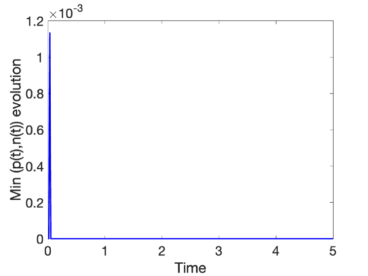
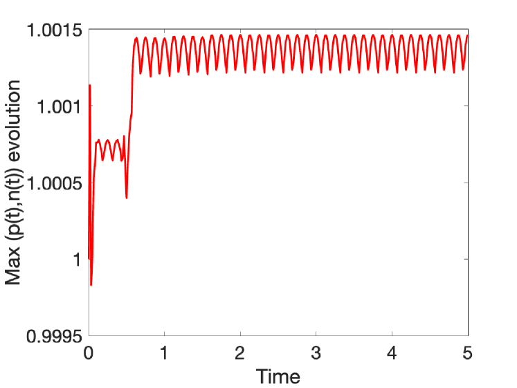
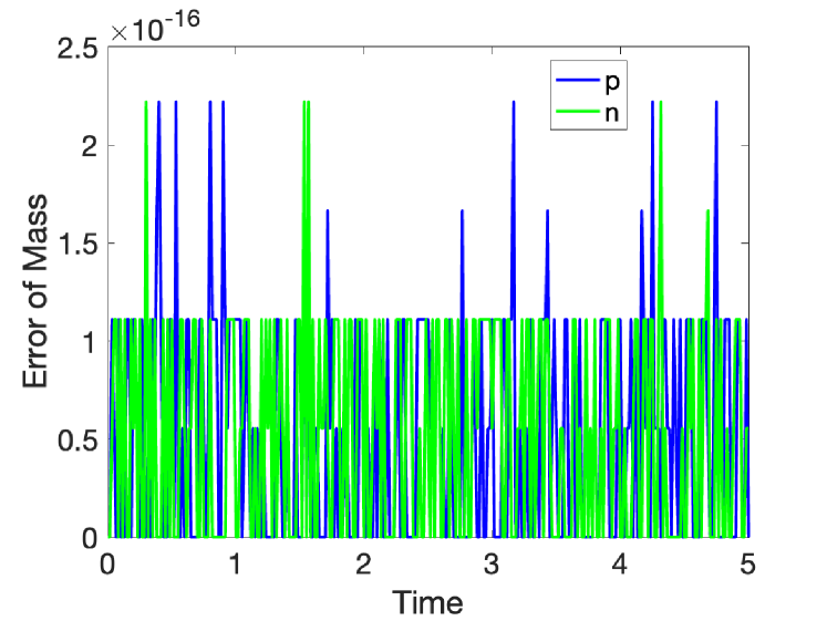
Figure 1: (Example 5.1 with CNFDP) Left: Lower bounds of $(n,p)$. Middle: Upper bounds of $(n,p)$. Right: Conservation of discrete masses for $p$ and $n$.

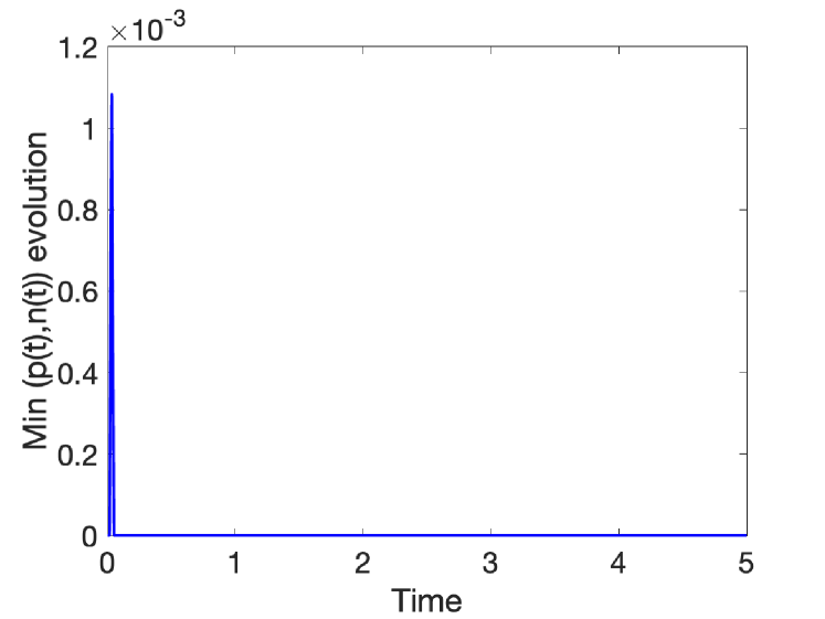
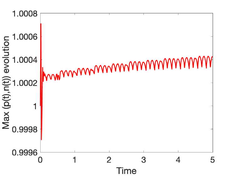
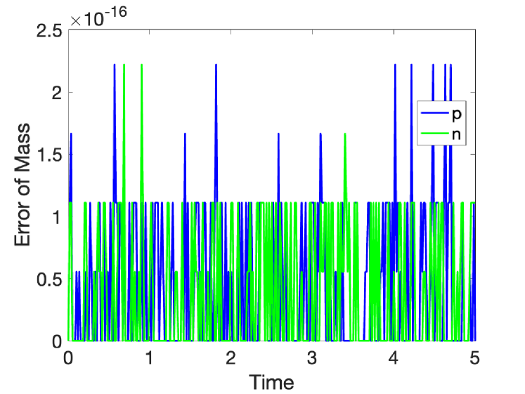
Figure 2: (Example 5.1 with CNFDP2) Left: Lower bounds of $(n,p)$. Middle: Upper bounds of $(n,p)$. Right: Conservation of discrete masses for $p$ and $n$.

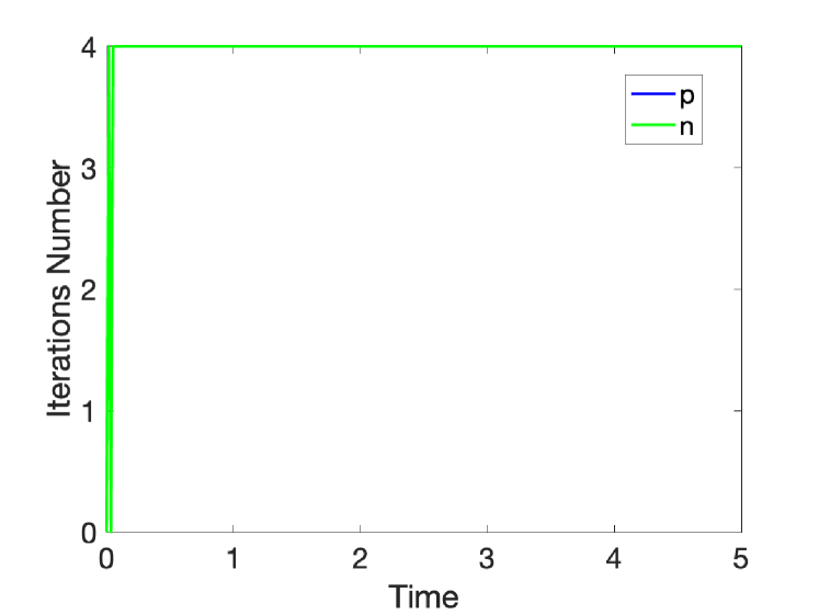
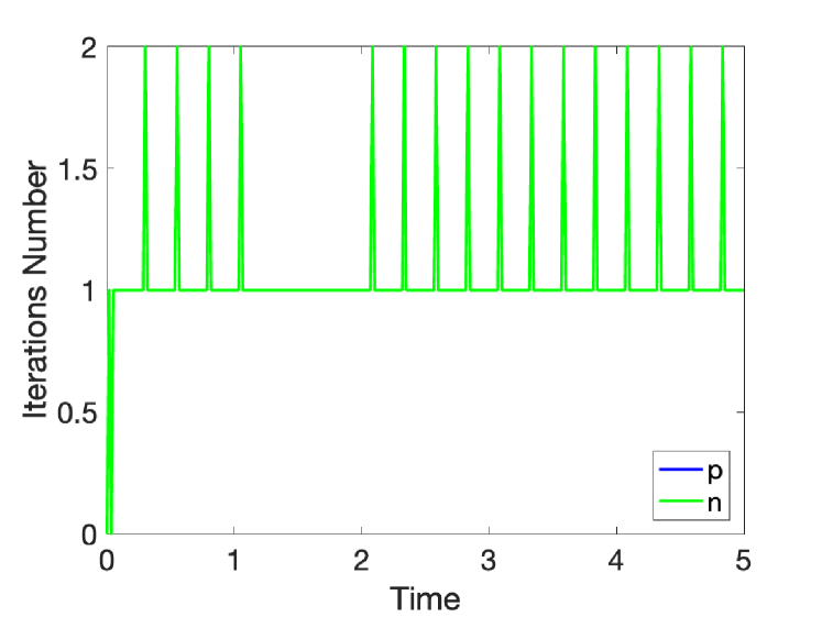
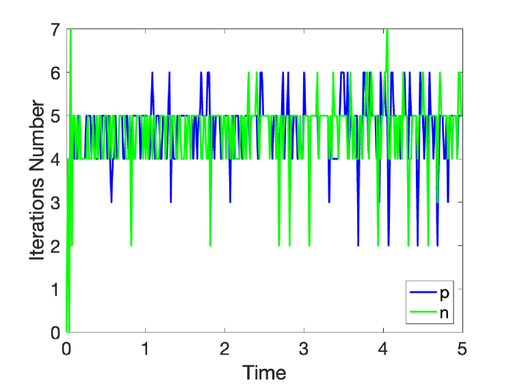
Figure 3: Number of iterations in the KKT condition solvers for Example 5.1. Left: the secant method with CNFDP. Middle: the semi smooth Newton method with CNFDP. Right: the semi smooth Newton method with CNFDP2.

5.2 Extension to homogeneous Neumann boundary conditions

Example 5.2.

We consider PNP (1) posed on $\Omega=[-2,2]^{2}$ with homogeneous Neumann boundary conditions and initial conditions

$$(p(x,y,0),n(x,y,0))=\left\{\begin{array}[]{ll}(1,0.5),&(x-0.5)^{2}+(y-0.5)^{2}\leq 0.25,\\ (0.5,1),&(x+0.5)^{2}+(y+0.5)^{2}\leq 0.25,\\ (0,0),&\text{ otherwise}.\end{array}\right.$$

Here, CNFDP is extended to investigate Example 5.2 with $\tau=4/200$ and $h=4/128$, where the finite difference treatment on the Neumann boundary conditions is done following [3, 15].

Figs. 4 and 5 depicts the evolution of $p$, $n$ and $\phi$ along with time, where positivity preserving and mass conservation for $p$ and $n$ are clearly observed. In addition, the total energy (6) and the electric energy (7) are decreasing in time.

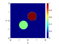
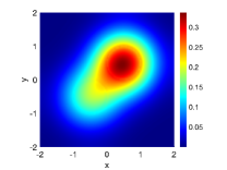
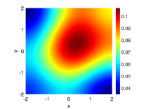
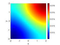
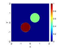
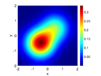
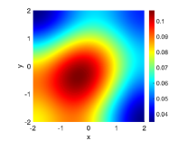
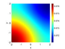
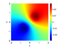
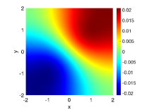
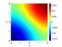
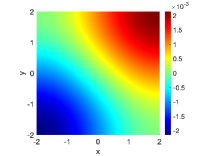
Figure 4: Example 5.2 with CNFDP. Snapshots of $p$, $n$ and $\phi$ (from top to bottom) at $t=0,0.04,0.2,1$ (from left to right), respectively.

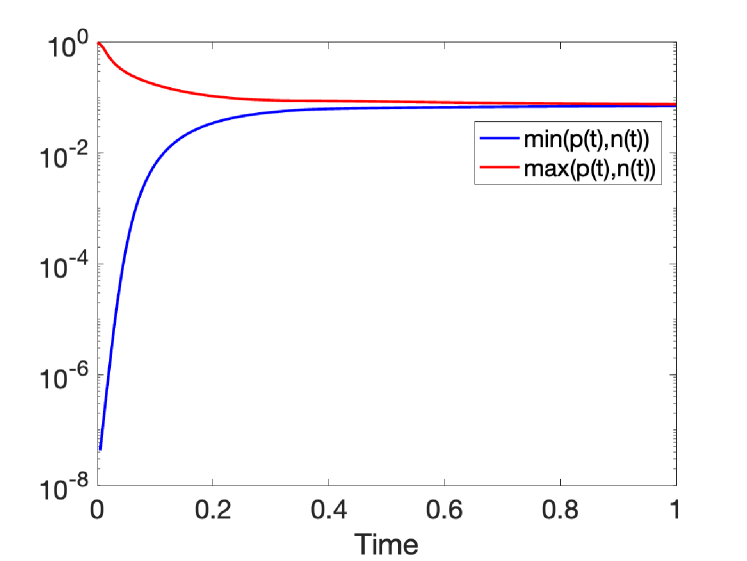
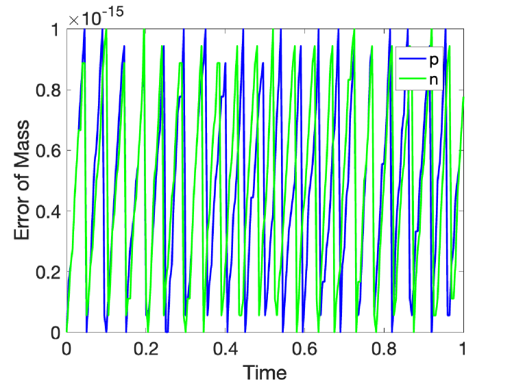
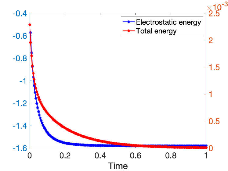
Figure 5: (Example 5.2 with CNFDP) Left: lower and upper bounds of $(n,p)$. Middle: error of discrete mass for $p$ and $n$. Right: evolution of total energy (6) and the electric potential energy (7).

5.3 3D case

Example 5.3.

The PNP system (1) with fixed charges on $\Omega=[-1,1]^{3}$ with periodic boundary conditions, i.e. the electric potential equation is replaced by

(50) $$-\Delta\phi=p-n+\rho,$$

where the external fixed charge distribution $\rho$ is given by

$$\rho(x,y,z) =200\sum\limits_{\varepsilon_{x},\varepsilon_{y},\varepsilon_{z}=\pm 1}\varepsilon_{x}\varepsilon_{y}\varepsilon_{z}e^{-100[(x+\varepsilon_{x}x_{i})^{2}+(y+\varepsilon_{y}y_{i})^{2}+(z+\varepsilon_{z}z_{i})^{2}]}.$$

The initial data is chosen as $p(x,y,z,0)=0.1$ and $n(x,y,z,0)=0.1$.

We simulate Example 5.3 using CNFDP with $\tau=2/100$ and $h=1/32$. The initial distribution of electrostatic potential $\phi$ (or the distribution of the fixed charges’ potential) is obtained by solving the Poisson equation with initial concentrations. Fig. 6 shows the snapshots of the concentrations $p$ and $n$ and electric potential $\phi$ at different times. As time evolves, the mobile ions are attracted by opposite fixed charges. Meanwhile, the electrostatic potential of the fixed charges is gradually screened by accumulated mobile ions of opposite signs. From Fig. 7, we can observe the point-wise bounds of $(n,p)$, the discrete mass, the total energy (6) and the electric potential energy (7), which confirms that CNFDP is positivity preserving and mass conserving. In addition, the energies (6) and (7) decrease monotonically in time.

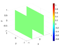
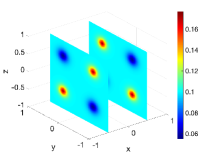
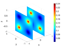
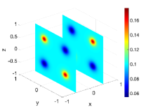
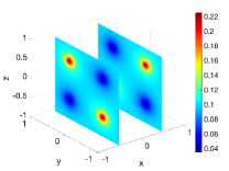
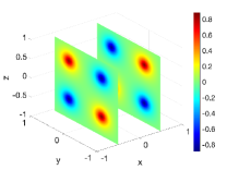
Figure 6: Example 5.3 with CNFDP. Snapshots of $p$, $n$ and $\phi$ (from top to bottom) at $t=0,0.01,0.05,2.0$ (from left to right), respectively.

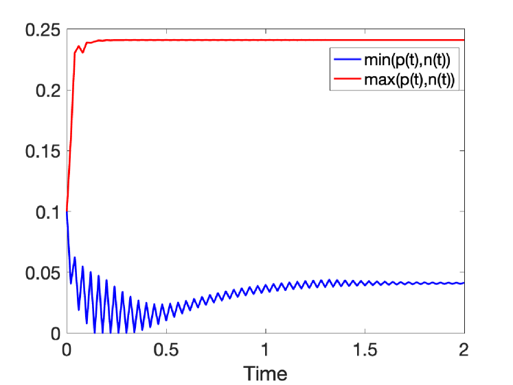
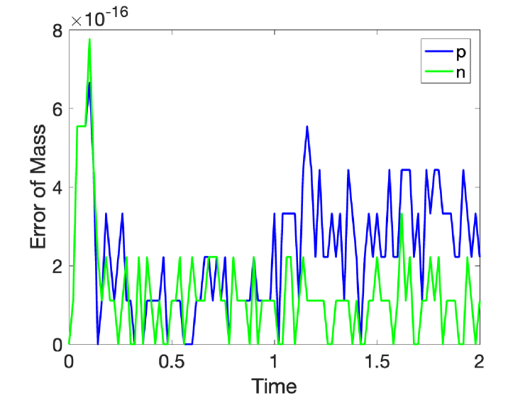
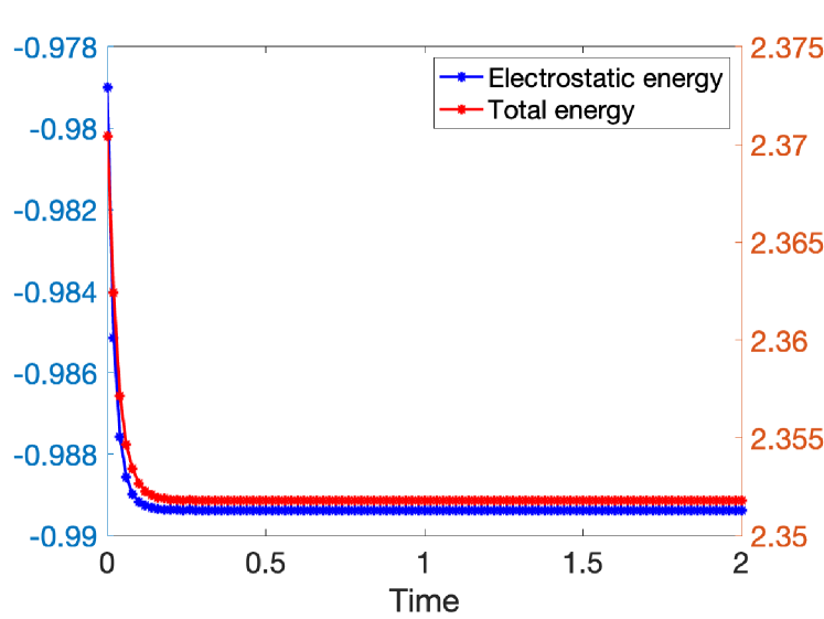
Figure 7: Example 5.3. Left: lower and upper bounds of (n,p). Middle: the error of discrete mass for $p$ and $n$. Right: the total energy (6) and the electric potential energy (7).

6 Conclusion

In this work, we developed efficient numerical schemes CNFDP and CNFDP2 to simulate the PNP equation (1), with positivity preserving and mass conservation at the discrete level. The key idea is to solve a minimization problem to project (correct) the intermediate solution to satisfy the desired physically constraints. By projection idea, either in $L^{2}$ norm (CNFDP) or $H^{1}$ norm (CNFDP2), the positivity and mass conservation of the numerical solutions can be guaranteed. For CNFDP, error estimates were shown to be at $O(\tau^{2}+h^{2})$ for the ion densities in $L^{2}$ norm and for the electric potential in $H^{1}$ norm. The proposed method with projection technique is a linearized scheme, which can be implemented very efficiently, with negligible computational cost in solving a nonlinear algebraic system. The method can be directly generalized to the case of multi-ions PNP system without any difficulty. Extension of the techniques and ideas to other more complex problems or higher order methods will be subject to future investigation.

Appendix

In this Appendix, we briefly describe the process about how to determine the Lagrange multipliers $\lambda^{k+1}_{h}(\mathbf{x}),\eta^{k+1}_{h}(\mathbf{x})\in X$ and $\xi^{k+1},\gamma^{k+1}\in\mathbb{R}$.

$L^{2}$ projection (15). From the complementary relaxation conditions (15), we can obtain numerical solutions $p_{h}^{k+1}$ and $n_{h}^{k+1}$ expressed as

(51) $$(p_{h}^{k+1},\lambda_{h}^{k+1})=\left\{\begin{array}[]{ll}\left[\tilde{p}_{h}^{k+1}-\xi^{k+1},0\right],&\text{ if }\tilde{p}_{h}^{k+1}-\xi^{k+1}>0,\\ \left[0,-(\tilde{p}_{h}^{k+1}-\xi^{k+1})\right],&\text{ otherwise},\end{array}\right.$$

and

(52) $$(n_{h}^{k+1},\eta_{h}^{k+1})=\left\{\begin{array}[]{ll}\left[\tilde{n}_{h}^{k+1}-\gamma^{k+1},0\right],&\text{ if }\tilde{n}_{h}^{k+1}-\gamma^{k+1}>0,\\ \left[0,-(\tilde{n}_{h}^{k+1}-\gamma^{k+1})\right],&\text{ otherwise,}\end{array}\right.$$

where the Lagrange multipliers $\xi^{k+1},\gamma^{k+1}\in\mathbb{R}$ are determined by the mass constraints, e.g. for $\xi^{k+1}$,

$$h^{2}\sum_{0<\tilde{p}_{h}^{k+1}(\mathbf{x})-\xi^{k+1}}\left(\tilde{p}_{h}^{k+1}(\mathbf{x})-\xi^{k+1}\right)=\langle{p}^{0}_{h},1\rangle.$$

Hence $\xi^{k+1}\in\mathbb{R}$ is the solution to the nonlinear algebraic equation

(53) $$F(\xi^{k+1})=h^{2}\sum_{i,j=1}^{N}\left(\tilde{p}_{h}^{k+1}(\mathbf{x}_{i,j})-\xi^{k+1}\right)^{+}-\langle{p}^{0}_{h},1\rangle=0,$$

where $f^{+}=\max\{f,0\}$ for $f\in\mathbb{R}$. Semi-smooth Newton methods [21, 10] can be employed to solve (53), i.e. for some initial guess $\xi_{0}\in\mathbb{R}$, find the root of $F(\xi)=0$ by updating

(54) $$\xi_{s+1}=\xi_{s}-V^{-1}(\xi_{s})F\left(\xi_{s}\right),\quad s=0,1,\cdots,$$

where $V(\xi_{s})$ is a generalized derivate in semi-smooth Newtown methods as

$$V(\xi_{s})=-h^{2}\sum_{i,j=1}^{N}\text{sgn}((\tilde{p}_{h}^{k+1}(\mathbf{x}_{i,j})-\xi_{s})^{+}),$$

and $\text{sgn}(\cdot)$ is the sign function with $\text{sgn}(s)=1$ ($s>0$), $\text{sgn}(0)=0$ and $\text{sgn}(s)=-1$ ($s<0$). Noticing $\xi^{k+1}$ is supposed to be of small magnitude [7] and $\xi^{k+1}\geq 0$ (Lemma 2.4), we can choose $\xi_{0}=0$ to start the semi-smooth Newton iterations. Once $\xi^{k+1}$ is known, we can update $\left(p_{h}^{k+1},\lambda_{h}^{k+1}\right)$ according to (51). $\gamma^{k+1}$ and $n_{h}^{k+1}$ can be computed in the same way. In all our numerical experiments, (54) converges in only one iteration so that the cost of solving (53) is negligible. The secant method can be also used to solve (53) [7].

$H^{1}$ projection (47)-(48). We present a semi-smooth Newton method to find the Lagrange multipliers $\lambda^{k+1}_{h}(\mathbf{x}),\eta^{k+1}_{h}(\mathbf{x})\in X$ and $\xi^{k+1},\gamma^{k+1}\in\mathbb{R}$ under $H^{1}$ projection. The KKT condition (47)-(48) for $\lambda^{k+1}$ and $\xi^{k+1}$ can be transformed to an equivalent system as follows

(55) $$F_{1}(U,\xi;\mathbf{x})=-\Delta_{h}{U}^{+}(\mathbf{x})+U(\mathbf{x})+\xi^{k+1}-(I-\Delta_{h})\tilde{p}^{k+1}_{h}(\mathbf{x})=0,\quad\mathbf{x}\in\Omega_{h},$$

$$F_{2}(U,\xi)=h^{2}\sum_{i,j=1}^{N}{U}^{+}(\mathbf{x}_{i,j})-M_{0}=0,$$

where $U(\mathbf{x})=U^{+}(\mathbf{x})-U^{-}(\mathbf{x})$ , $U^{+}=\max(U^{k+1}(\mathbf{x}),0)$, $U^{-}=\max(-U^{k+1}(\mathbf{x}),0)$, and $U^{+}(\mathbf{x})={p}^{k+1}_{h}(\mathbf{x})$, $U^{-}(\mathbf{x})=\lambda_{h}^{k+1}(\mathbf{x})$. $\eta^{k+1}$ and $\gamma^{k+1}$ can be solved in the same way.

The semi-smooth Newton method can be applied to solve (55). We start with the generalized Jacobian to be used in the semi-smooth Newton iterations. In a simplified form, at $(U(\mathbf{x}),\xi)\in X\times\mathbb{R}$, the generalized Jacobian $J$ (acting on a vector $(V(\mathbf{x}),\zeta)\in X\times\mathbb{R}$) can be written as

(56) $$J\begin{pmatrix}V(\mathbf{x})\\ \zeta\end{pmatrix}=\begin{pmatrix}I-\Delta_{h}\left(\text{sgn}(U^{+}(\mathbf{x}))V(\mathbf{x})\right)+\zeta\\ h^{2}\sum(\text{sgn}(U^{+}(\mathbf{x}))V(\mathbf{x})\end{pmatrix}.$$

By a careful computation based on (55)-(56), a semi-smooth Newton method for solving (55) with initial $\xi_{0}$ and $U_{0}(\mathbf{x})$ can be designed as follows:

$$\xi_{s+1}= \xi_{s}+\frac{F_{2}(U_{s},\xi_{s})+h^{2}\sum_{i,j=1}^{N}\text{sgn}(U_{s}^{+}(\mathbf{x}_{i,j}))V_{1}(\mathbf{x}_{i,j})}{h^{2}\sum\limits_{i,j=1}^{N}(\text{sgn}(U^{+}_{s}(\mathbf{x}_{i,j}))V_{2}(\mathbf{x}_{i,j})},$$

$$U_{s+1}= U_{s}+V_{s}-(\xi_{s+1}-\xi_{s})V_{2},$$

where $V_{1}(\mathbf{x})=(I-\Delta_{h}\text{sgn}(U_{s}^{+}))^{-1}(-F_{1}(U_{s},\xi_{s}))$ (by abuse of notation) and $V_{2}(\mathbf{x})=(I-\Delta_{h}\text{sgn}(U_{s}^{+}))^{-1}\mathbf{1}($ ($\mathbf{1}$ is the constant $1$ function on $\Omega_{h}$). For solving $V_{1}$ and $V_{2}$, we can use $(I-\Delta_{h})^{-1}$ as a pre-conditioner. When Newton iteration converges for some $s\geq 0$, we have $p^{k+1}(\mathbf{x})=U^{+}_{s+1}(\mathbf{x})$. To start the semi-smooth Newton iteration, we may set $\xi_{0}=0$ and $U_{0}(\mathbf{x})=\tilde{p}^{k+1}_{h}(\mathbf{x})$.

References

- [1] L. Ambrosio, N. Gigli, and G. Savaré, Gradient Flows:In Metric Spaces and in the Space of Probability Measures, Lectures in Mathematics. ETH Zürich, 2 ed., 2008.
- [2] P. Biler, W. Hebisch, and T. Nadzieja, The Debye system: existence and large time behavior of solutions, Nonlinear Analysis: Theory, Methods & Applications, 23 (1994), pp. 1189–1209.
- [3] Y. Cai, J. Chen, C. Wang, and C. Xie, A second-order numerical method for Landau-Lifshitz-Gilbert equation with large damping parameters, Journal of Computational Physics, 451 (2022), p. 110831.
- [4] Y. Cai and J. Shen, Error estimates for a fully discretized scheme to a Cahn-Hilliard phase-field model for two-phase incompressible flows, Mathematics of Computation, 87 (2018), pp. 2057–2090.
- [5] J. Cartailler, Z. Schuss, and D. Holcman, Analysis of the Poisson-Nernst-Planck equation in a ball for modeling the voltage-current relation in neurobiological microdomains, Physica D: Nonlinear Phenomena, 339 (2017), pp. 39–48.
- [6] Q. Cheng and J. Shen, Global constraints preserving scalar auxiliary variable schemes for gradient flows, SIAM Journal on Scientific Computing, 42 (2020), pp. A2489–A2513.
- [7] Q. Cheng and J. Shen, A new lagrange multiplier approach for constructing structure preserving schemes, I. Positivity preserving, Computer Methods in Applied Mechanics and Engineering, 391 (2022), p. 114585.
- [8] Q. Cheng and J. Shen, A new lagrange multiplier approach for constructing structure preserving schemes, II. Bound preserving, SIAM Journal on Numerical Analysis, 60 (2022), pp. 970–998.
- [9] J. Ding, Z. Wang, and S. Zhou, Positivity preserving finite difference methods for Poisson-Nernst-Planck equations with steric interactions: Application to slit-shaped nanopore conductance, Journal of Computational Physics, 397 (2019), p. 108864.
- [10] F. Facchinei and J.-S. Pang, Finite-dimensional variational inequalities and complementarity problems,Volume II, Springer New York, NY, 2003.
- [11] A. Flavell, M. Machen, B. Eisenberg, J. Kabre, C. Liu, and X. Li, A conservative finite difference scheme for Poisson-Nernst-Planck equations, Journal of Computational Electronics, 13 (2014), pp. 235–249.
- [12] G. Fu and Z. Xu, High-order space-time finite element methods for the Poisson-Nernst-Planck equations: Positivity and unconditional energy stability, Computer Methods in Applied Mechanics and Engineering, 395 (2022), p. 115031.
- [13] H. Gajewski and K. Gröger, On the basic equations for carrier transport in semiconductors, Journal of Mathematical Analysis and Applications, 113 (1986), pp. 12–35.
- [14] D. He and K. Pan, An energy preserving finite difference scheme for the Poisson-Nernst-Planck system, Applied Mathematics and Computation, 287-288 (2016), pp. 214–223.
- [15] D. He, K. Pan, and X. Yue, A positivity preserving and free energy dissipative difference scheme for the Poisson-Nernst-Planck system, Journal of Scientific Computing, 81 (2019), pp. 436–458.
- [16] J. G. Heywood and R. Rannacher, Finite-element approximation of the nonstationary Navier-Stokes problem. Part IV: Error analysis for second-order time discretization, SIAM Journal on Numerical Analysis, 27 (1990), pp. 353–384.
- [17] C.-Y. Hsieh and Y. Yu, Existence of solutions to the Poisson-Nernst-Planck system with singular permanent charges in , SIAM Journal on Mathematical Analysis, 54 (2022), pp. 1223–1240.
- [18] J. Jerome, Consistency of semiconductor modeling: An existence/stability analysis for the stationary van roosbroeck system, SIAM Journal on Applied Mathematics, 45 (1985), pp. 565–590.
- [19] M. Kilic, M. Z. Bazant, and A. Ajdari, Steric effects in the dynamics of electrolytes at large applied voltages. II. modified Poisson-Nernst-Planck equations, Physical review. E, Statistical, nonlinear, and soft matter physics, 75 (2007), p. 021503.
- [20] D. Kinderlehrer, L. Monsaingeon, and X. Xu, A wasserstein gradient flow approach to Poisson-Nernst-Planck equations, ESAIM: Control, Optimisation and Calculus of Variations, 23 (2015), pp. 137–164.
- [21] M. Kojima and S. Shindo, Extension of newton and quasi-newton methods to systems of equations, Journal of The Operations Research Society of Japan, 29 (1986), pp. 352–375.
- [22] B. Li, J. Yang, and Z. Zhou, Arbitrarily high-order exponential cut-off methods for preserving maximum principle of parabolic equations, SIAM Journal on Scientific Computing, 42 (2020), pp. A3957–A3978.
- [23] C. Liu, C. Wang, S. M. Wise, X. Yue, and S. Zhou, A positivity-preserving, energy stable and convergent numerical scheme for the poisson-nernst-planck system, Mathematics of Computation, 90 (2020), pp. 2071–2106.
- [24] H. Liu, Z. Wang, P. Yin, and H. Yu, Positivity-preserving third order DG schemes for Poisson-Nernst-Planck equations, Journal of Computational Physics, 452 (2022), p. 110777.
- [25] B. Lu, M. J. Holst, J. Andrew McCammon, and Y. Zhou, Poisson–Nernst–Planck equations for simulating biomolecular diffusion-reaction processes I: Finite element solutions, Journal of Computational Physics, 229 (2010), pp. 6979–6994.
- [26] C. Lu, W. Huang, and E. S. Van Vleck, The cutoff method for the numerical computation of nonnegative solutions of parabolic pdes with application to anisotropic diffusion and Lubrication-type equations, Journal of Computational Physics, 242 (2013), pp. 24–36.
- [27] J. Lyu, C.-C. Lee, and T.-C. Lin, Near- and far-field expansions for stationary solutions of Poisson‐Nernst‐Planck equations, Mathematical Methods in the Applied Sciences, 44 (2021), pp. 10837 – 10860.
- [28] P. A. Markowich, C. A. Ringhofer, and C. Schmeiser, Semiconductor equations, Springer Vienna, 1 ed., 1990.
- [29] M. S. Metti, J. Xu, and C. Liu, Energetically stable discretizations for charge transport and electrokinetic models, Journal of Computational Physics, 306 (2016), pp. 1–18.
- [30] M. S. Mock, On equations describing steady‐state carrier distributions in a semiconductor device, Communications on Pure and Applied Mathematics, 25 (1972), pp. 781–792.
- [31] W. Nernst, Die elektromotorische wirksamkeit der jonen, Zeitschrift für Physikalische Chemie, 4 (1889), pp. 129–181.
- [32] B. Piotr, H. Danielle, and N. Tadeusz, Existence and nonexistence of solutions for a model of gravitational interaction of particles, II, Colloquium Mathematicae, 67 (1994), pp. 297–308.
- [33] B. Piotr and N. Tadeusz, Existence and nonexistence of solutions for a model of gravitational interaction of particles, I, Colloquium Mathematicae, 66 (1993), pp. 319–334.
- [34] M. Planck, Ueber die erregung von electricität und wärme in electrolyten, Annalen der Physik, 275 (1890), pp. 161–186.
- [35] A. Prohl and M. Schmuck, Convergent discretizations for the Nernst-Planck-Poisson system, Numerische Mathematik, 111 (2009), pp. 591–630.
- [36] M. Schmuck, Analysis of the Navier-Stokes-Nernst-Planck-Poisson system, Mathematical Models and Methods in Applied Sciences, 19 (2009), pp. 993–1014.
- [37] J. Shen, On error estimates of projection methods for Navier-Stokes equations: First-order schemes, SIAM Journal on Numerical Analysis, 29 (1992), pp. 57–77.
- [38] J. Shen and J. Xu, Unconditionally positivity preserving and energy dissipative schemes for Poisson-Nernst-Planck equations, Numerische Mathematik, 148 (2021), pp. 671–697.
- [39] Z. Song, X. Cao, and H. Huang, Electroneutral models for dynamic Poisson-Nernst-Planck systems, Physical Review E, 97 (2018), p. 012411.
- [40] R. Temam, Une méthode d’approximation de la solution des équations de navier-stokes, Bulletin de la Société Mathématique de France, 96 (1968), pp. 115–152.
- [41] J. J. W. van der Vegt, Y. Xia, and Y. Xu, Positivity preserving limiters for time-implicit higher order accurate discontinuous galerkin discretizations, SIAM Journal on Scientific Computing, 41 (2019), pp. A2037–A2063.
- [42] Y. Wang, C. Liu, and Z. Tan, A generalized Poisson-Nernst-Planck-Navier-Stokes model on the fluid with the crowded charged particles: Derivation and its well-posedness, SIAM Journal on Mathematical Analysis, 48 (2016), pp. 3191–3235.
- [43] J. Yang, Z. Yuan, and Z. Zhou, Arbitrarily high-order maximum bound preserving schemes with cut-off postprocessing for Allen-Cahn equations, Journal of Scientific Computing, 90 (2022), pp. 1–36.
- [44] Q. Zhang, Q. Wang, L. Zhang, and B. Lu, A class of finite element methods with averaging techniques for solving the three-dimensional drift-diffusion model in semiconductor device simulations, Journal of Computational Physics, 458 (2022), p. 111086.
- [45] Y. Zhu, S. Xu, R. S. Eisenberg, and H. Huang, A tridomain model for potassium clearance in optic nerve of necturus, Biophysical Journal, 120 (2021), pp. 3008–3027.