Relative alignment between gas structures and magnetic field in Orion A at different scales using different molecular gas tracers

Abstract

Context. Magnetic fields can play crucial roles in high-mass star formation. Nonetheless, the significance of magnetic fields at various scales and their relationship with gas structures is largely overlooked.

Aims. Our goal is to examine the relationship between the magnetic field and molecular gas structures within the Orion A giant molecular cloud at different scales and density regimes.

Methods. We assess the gas intensity structures and column densities in Orion A by utilizing ¹²CO, ¹³CO, and C¹⁸O from Nobeyama observations. Through comparing Nobeyama observations with Planck polarization observations on large scales ($\sim 0.6$ pc) and JCMT polarization observations on small scales ($\sim 0.04$ pc), we investigate how the role of magnetic fields change with scale and density.

Results. We find a similar trend from parallel to perpendicular alignment with increasing column densities in Orion A at both large and small spatial scales. Besides, when changing from low-density to high-density tracers, the relative orientation preference changes from random to perpendicular. The self-similar results at different scales indicate that magnetic fields are dynamically important in both cloud formation and filament formation. However, magnetic fields properties at small scales are relative complicated, and the interplay between magnetic field and star-forming activities needs to be discussed case-by-case.

1 Introduction

The formation and evolution of molecular clouds are intricate processes driven by the interplay of several crucial factors, which include gravity, turbulence, magnetic fields, thermal instability, feedback, and cosmic-ray ionization. They play different roles in different activities such as filamentary structure formation and star formation process (e.g., Bergin & Tafalla 2007; McKee & Ostriker 2007; Wang 2015). The magnetic field is considered as one of the key components in slowing down the star formation rate, but it is difficult to measure the magnetic field because of observational limitations (Hennebelle & Falgarone 2012).

Till now, there are two primary methods for measuring magnetic field in molecular clouds. The observation of Zeeman effect is the only direct way to measure the strength of magnetic field in interstellar clouds. Some observations have succeeded in calculating the value of magnetic fields along the line of sight (e.g., Crutcher et al. 1996; Falgarone et al. 2008). However, because the Doppler broadening effect is always larger than Zeeman splitting effect, this method is limited by observational techniques and can not be widely used (Crutcher 2012).

An alternative way to infer the morphology of magnetic fields is through the observations of linear polarization induced by interstellar dust. One possible and longstanding method is to measure the polarization from the background starlight, which assumes aspherical dust grains align with their long axis perpendicular to the local magnetic field and produce polarization parallel to the field projected on the plane of sky (see Andersson et al. 2015 for a review). However, it is difficult to reproduce the projected magnetic field morphology fully inside molecular clouds. In recent years, a more general method to measure the orientation of magnetic fields within the molecular clouds is through the measurement of linearly polarized radiation emitted from dust, which can map the morphology of magnetic fields on the plane of sky on small scales around the star-forming regions (e.g., Matthews et al. 2009; Zhang et al. 2014) or on large scales across the whole sky (Planck Collaboration et al. 2020a), helping us to know more about magnetic fields.

The strength of the magnetic field projected on the plane of sky can be estimated using the Davis-Chandrasekhar-Fermi method (Davis 1951; Chandrasekhar & Fermi 1953), but the uncertainty and applicability of the DCF method are always discussed (e.g., Liu et al. 2021; Skalidis & Tassis 2021; Skalidis et al. 2021; Chen et al. 2022). Some studies seek to derive additional information about the role of magnetic field by comparing the relative orientation of magnetic field inferred from dust polarization with the orientation of molecular cloud structures, which find strong correlation between magnetic field morphology and the geometry of the molecular cloud structures (e.g., Tassis et al. 2009; Koch et al. 2013; Planck Collaboration et al. 2016a, b). Multiscale magnetic fields are also explored in different researches, suggesting that the role of the magnetic field may vary at different scales (e.g., Li et al. 2015; Chen et al. 2020; Liu et al. 2023).

In recent years, the histograms of relative orientation (HRO) technique is introduced to compare the relative orientation between column density structures and magnetic field (Soler et al. 2013). Applying this method to observations, the transition from parallel to perpendicular with increasing column density has been found, indicating that the magnetic field plays an important role for the gas dynamics at cloud scales (Planck Collaboration et al. 2016b; Soler et al. 2017).

A more detailed study attempts to connect the intensity structure of molecular lines from different gas tracers with the magnetic field in Vela C Giant Molecular Cloud (Fissel et al. 2019). When comparing the results with different tracers, the authors find a transition from parallel to perpendicular as the critical density of the tracers increases, indicating a correlation between gas intensity structures and magnetic fields, which is consistent with the result of recent Magnetohydrodynamics (MHD) simulations (Mazzei et al. 2023). However, it is just a case study, and the findings in this work need to be examined in a larger sample.

The Orion Giant Molecular Cloud is the nearest high-mass star forming region (d=414 pc, Menten et al. 2007), which is well known for its hierarchical filamentary structure and strong star-forming activities (Bally 2008). Magnetic field properties in Orion A are deeply investigated both on large scales (e.g., Houde et al. 2004; Clark & Johnson 1974) and small scales (e.g., Poidevin et al. 2010; Pattle et al. 2017; Soler 2019). In this work, we aim at examining the relationship between molecular gas structure and magnetic field at different scales. We make use of the spectral cube of three different molecular lines and then calculate different gas intensity structure maps to make a comparison with the magnetic field. Our goal is to find whether there is similar trend in relative orientation with the increasing column density within Orion A Giant Molecular Cloud, whether the correlation between gas structures and magnetic field change when comparing them at different scales, and whether there are clear differences in relative orientation when using different gas tracers.

We first introduce Nobeyama-, SCUPOL- and Planck- derived maps used in our analysis in Sect. 2. The methods of calculation and the results are described in Sect. 3. We show the main results in Sect. 4. In Sect. 5, we compare our results with the previous study and discuss the implications of our work. A brief summary of our results is given in Sect. 6.

2 Observations

2.1 Planck dust polarization data

For the analyses in this work, we calculate the magnetic field orientations from linearly polarized dust emission. Planck observations provide the linear polarization maps (Stokes Q and U) from 30 to 353 GHz in multiple frequency bands across the entire sky (Planck Collaboration et al. 2020a). These maps serve as valuable tools for studying polarized emission from interstellar dust. On large scales we adopt the publicly available PR3 data from the High-Frequency Instrument (HFI; Lamarre et al. 2010) at 353 GHz (Planck Collaboration et al. 2020b). The maps of Stokes Q and U are initially at 5^′ spatial resolution ($\sim 0.6$ pc) and the pixel size of 1.71^′. We calculate the polarization position angle projected on the plane of sky from the Stokes parameters as

$$\theta_{\mathrm{p}}^{\mathrm{g}}=\frac{1}{2}\arctan(U,Q)$$ (1)

The magnetic field position angle can be obtained by adding 90^∘ to the polarization angle: $\theta_{\mathrm{B}}^{\mathrm{g}}=\theta_{\mathrm{p}}^{\mathrm{g}}+\frac{\pi}{2}$. The downloaded Planck Q and U maps are in galactic coordinates and the polarization position angle in equatorial coordinates can be derived using $\theta_{\mathrm{p}}^{\mathrm{e}}=\theta^{\mathrm{g}}_{\mathrm{p}}-\Delta\theta_{\mathrm{p}}^{\mathrm{g}-\mathrm{e}}$, where

$$\Delta\theta^{\mathrm{g-e}}_{\mathrm{p}}=\arctan[\frac{\cos\left(l-32.9^{\circ}\right)}{\cos b\cot 62.9^{\circ}-\sin b\sin\left(l-32.9^{\circ}\right)}]$$ (2)

is the angle difference between galactic and equatorial coordinates (Corradi et al. 1998). The debiased polarization intensity $PI$ and the corresponding uncertainties $\sigma_{PI}$ can be derived using the modified asymptotic estimator (pMAS; Plaszczynski et al. 2014). The rms noise level of stokes Q and U map is similar, with a value of 0.26 $\mathrm{mK_{CMB}}$ (hereafter $\sigma_{QU})$. In our analysis we only use the polarization data with enough signal-to-noise ratio ($PI/\sigma_{PI}>3$). The uncertainties of polarization position angle can be calculated using $\sigma_{\theta}\sim\frac{\sigma_{QU}}{2}\sqrt{{1}/{(Q^{2}+U^{2})}}$.

2.2 JCMT dust polarization data

On small scales we use the data to measure relative orientation of magnetic field from the JCMT/SCUPOL catalog (Matthews et al. 2009). This catalog is a combination of calibrated and reduced data observed between 1997 to 2005 at 850 $\mu$m by the polarimeter for Submillimeter Common-User Bolometer Array (SCUBA) on the James Clerk Maxwell Telescope. There are two regions with high-resolution polarization data in Orion A region: OMC-1 and OMC-2/3. The individual observations were combined to create composite Stokes I, Q and U maps. The data are sampled on a 10^′′ per pixel grid in J2000 coordinates and the effective beam size of the map is 20^′′ ($\sim 0.04$ pc). We calculate the polarization position angle projected on the plane of sky from the Stokes parameters as

$$\theta_{\mathrm{p}}^{\mathrm{e}}=\frac{1}{2}\arctan(U,Q)$$ (3)

The derived position angle is in equatorial coordinates, and there is no need for transformation. We apply the same method mentioned in Sect. 2.1 to calculate the uncertainties and the rms noise of stokes Q and U maps is approximately 0.1 mJy/beam within OMC-1 and 0.03 mJy/beam within OMC-2/3.

2.3 Nobeyama molecular line data

To study the gas structures in Orion A, we select data from the NRO Star Formation Legacy Project, based on observations at the Nobeyama Radio Observatory (NRO). The observations covered ${}^{12}\mathrm{CO}$ ($J=1-0$), ${}^{13}\mathrm{CO}$ ($J=1-0$), $\mathrm{C}^{18}\mathrm{O}$ ($J=1-0$), $\mathrm{N}_{2}\mathrm{H}^{+}$ ($J=1-0$), CCS ($J_{N}=8_{7}-6_{7}$) lines toward some nearby star-forming regions (M17, Orion A and Aquila Rift). Detailed information of observations is summarized in Nakamura et al. (2019). In this paper, we use three different molecular lines with significant extended emission: ${}^{12}\mathrm{CO}$ (J=1-0), ${}^{13}\mathrm{CO}$ (J=1-0), $\mathrm{C}^{18}\mathrm{O}$ (J=1-0). The ${}^{12}\mathrm{CO}$, ${}^{13}\mathrm{CO}$, $\mathrm{C}^{18}\mathrm{O}$ data are convolved to 21.7^′′ beam size and reprojected to a common 7.5^′′$\times$7.5^′′ grid. The velocity resolution is $0.1\mathrm{\leavevmode\nobreak\ km}\mathrm{\leavevmode\nobreak\ s}^{-1}$ and the noise levels of ${}^{12}\mathrm{CO}$, ${}^{13}\mathrm{CO}$, $\mathrm{C}^{18}\mathrm{O}$ lines are at a range of $0.5-1.5$ K, $0.2-0.3$ K and $0.26-0.3$ K, respectively. For the sake of comparison with Planck observations, we use the maps smoothed to a angular resolution of 5^′, and we directly compare the map between SCUPOL and Nobeyama observations on small scales without smoothing because of similar angular resolution.

3 Methods

3.1 Detailed procedure of comparison

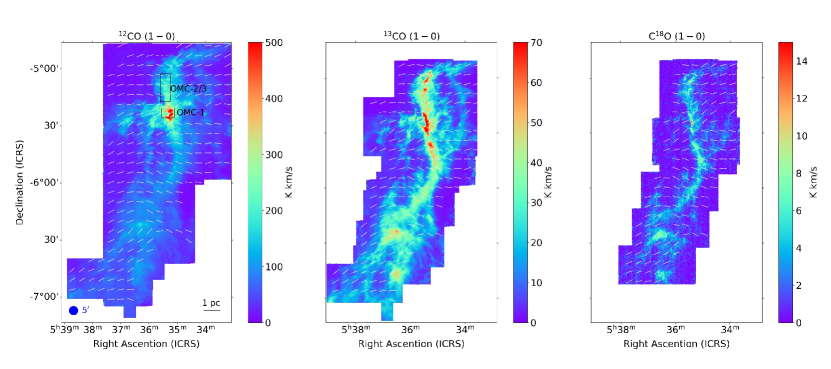
Figure 1: Nobeyama Moment-0 maps for ¹²CO, ¹³CO, C¹⁸O with the resolution of 21.7^′′. The white vectors represent the orientation of Planck magnetic fields. Only segments with enough signal-to-noise ratio are plotted (PI/$\sigma_{\mathrm{PI}}>$3). The blue circle in the bottom left marks the resolution of Planck magnetic fields. The black rectangles represent the specific regions with high-resolution polarization observations.

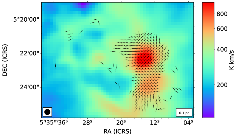
Figure 2: The magnetic field vectors overlaid on the ¹²CO moment-0 map of OMC-1. Only the segments with stokes I signal-to-noise ratio (S/N$>25$) and PI/$\sigma_{\mathrm{PI}}>$3 are plotted. The black circle in the bottom left marks the resolution of SCUPOL magnetic fields.

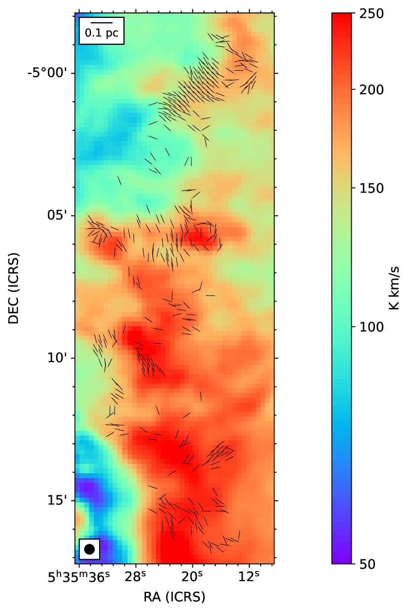
Figure 3: The magnetic field vectors overlaid on the ¹²CO moment-0 map of OMC-2/3. Only the segments with stokes I signal-to-noise ratio (S/N$>25$) and PI/$\sigma_{\mathrm{PI}}>$3 are plotted. The black circle in the bottom left marks the resolution of SCUPOL magnetic fields.

Here is the detailed procedure in our work. On large scales, we initially smoothed the spectral line data cube to match the angular resolution of Planck observations and then compared the relative orientation of gas intensity gradients with the polarization position angle (perpendicular to the magnetic field) at low angular resolution. In special regions with high-resolution SCUPOL polarization observations, we directly calculated the gradient vector field of each map and compared it with the orientation of polarization.

3.2 Column density maps

The 0th Moment map was created by integrating the emission between 0 and $18\mathrm{\leavevmode\nobreak\ km}\mathrm{\leavevmode\nobreak\ s}^{-1}$. To exclude the impacts of unreliable pixels, we selected pixels whose spectra exhibit at least five velocity channels with a brightness temperature greater than 8$\sigma$ for ${}^{12}\mathrm{CO}$, 5$\sigma$ for ${}^{13}\mathrm{CO}$, and 3$\sigma$ for $\mathrm{C}^{18}\mathrm{O}$. The derived moment-0 maps for Orion A region are shown in Fig. 1, and zoom-in ${}^{12}\mathrm{CO}$ moment-0 maps for OMC-1 and OMC-2/3 with overlaid JCMT-derived magnetic field vectors are shown in Figs. 2 and 3.

Previous studies show that the relative orientation between gas structures and magnetic field change from parallel to perpendicular with increasing column densities (e.g., Planck Collaboration et al. 2016b; Soler et al. 2017). In our study, we estimated the column density structures the using ${}^{12}\mathrm{CO}$ and ${}^{13}\mathrm{CO}$ lines (see detailed derivation from Mangum & Shirley 2015; Li et al. 2018, and references therein). Firstly, assuming LTE and ${}^{12}\mathrm{CO}$ line always optically thick, we calculated the excitation temperature of ${}^{12}\mathrm{CO}$ according to the following formula:

$$T_{\text{ex}}=5.532\left[\ln\left(1+\frac{5.532}{T_{\text{peak}}+0.819}\right)\right]^{-1}$$ (4)

where $T_{\text{peak}}$ is the maximum brightness temperature of the ${}^{12}\mathrm{CO}$ line. Then the optical depth of ${}^{13}\mathrm{CO}$ can be calculated as

$$\tau^{13}(v)=-\ln\left[1-\frac{T_{\mathrm{mb}}(^{13}\mathrm{CO})}{5.29}\left(\left[e^{5.29/T_{\mathrm{ex}}}-1\right]^{-1}-0.164\right)^{-1}\right]$$ (5)

where $T_{\mathrm{mb}}(^{13}\mathrm{CO})$ is the brightness temperature of the ${}^{13}\mathrm{CO}$ line. Assuming that the emission of ${}^{13}\mathrm{CO}$ is optically thin, we can use the approximate relation (Pineda et al. 2010):

$$T_{\mathrm{ex}}\int\tau dv\approx\frac{\tau_{0}}{1-e^{-\tau_{0}}}\int T_{\mathrm{mb}}dv$$ (6)

where $\tau_{0}$ is the peak optical depth of the ${}^{13}\mathrm{CO}$ emission line. Assuming $\mathrm{H_{2}}/{}^{13}\mathrm{CO}=7.1\times 10^{5}$ (Frerking et al. 1982), we can obtain the total column density of molecular hydrogen:

$$N(\mathrm{H}_{2})^{{}^{13}\mathrm{CO}}=1.72\times 10^{20}\frac{\tau_{0}}{1-e^{-\tau_{0}}}\\ \times\frac{1+0.88/T_{\mathrm{ex}}}{1-e^{-5.29/T_{\mathrm{ex}}}}\int T_{\mathrm{mb}}{(^{13}\mathrm{CO})}dv$$ (7)

One thing we must note is that the ${}^{13}\mathrm{CO}$ line might be optically thick in some dense regions within Orion A, but the derived column density maps were only used to examine the relation between the orientation and column density, which would not affect our results much.

3.3 Calculation of relative orientations

We determined the relative angle between the intensity structures and the magnetic field using similar methods described in Soler et al. (2013). The angle $\phi$, between the tangent to the local intensity structure contours and magnetic field, can be calculated using the following formula (Fissel et al. 2019):

$$\phi=\arctan\ (|\nabla I\times\theta_{\mathrm{p}}|,\nabla I\cdot\theta_{\mathrm{p}})$$ (8)

Here, $\theta_{\mathrm{p}}$ marks the polarization position angle, perpendicular to the orientation of magnetic fields. $\nabla I$ represents the orientation of the intensity gradient that is perpendicular to the contours of intensity. The relative orientation angle $\phi$ is within the range $[0^{\circ},90^{\circ}]$ and angle outside the range can be transformed to uniquely determined angle within the limit.

The gradient technique was employed to characterize the orientation of structures in a scalar field. Within nearby $3\times 3$ pixels, the gradient of gas intensity structures was derived using the similar method described in Sokolov et al. (2019). We utilized a first-degree bivariate polynomial function to describe the gradient field: $f(\alpha,\delta)=I_{0}+a\Delta\alpha+b\Delta\delta$, where $I_{0}$ represents the intensity of the central point, $\Delta\alpha$ and $\Delta\delta$ represent the pixel offsets. To ensure precision, only pixels with sufficient signal-to-noise ratio were included in the gradient analysis. In addition, we selected pixels with more than 7 good points in the nearby $3\times 3$ kernel size. A least-squares method was employed to derive the gradient field toward each pixel:

$$p({r})={\mathop{argmin}\limits_{a,b}{\sum_{\Delta\alpha,\Delta\delta\leq 1}{(I({r}^{\prime})-f({r}^{\prime},a,b))^{2}}}}$$ (9)

The orientation of gradient and its uncertainty can be given by $\nabla I=\arctan\ (b,a)$ and $\sigma_{\nabla I}=\frac{1}{a^{2}+b^{2}}\sqrt{a^{2}\sigma_{b}^{2}+b^{2}\sigma_{a}^{2}}$ (Planck Collaboration et al. 2016b).

We assessed the relative orientation of the magnetic field in relation to the gas structures using the HRO technique (Soler et al. 2013). The map was segmented into seven intensity bins, each containing an equal number of selected pixels based on their intensity values. We used 9 angle bins, each with a width of $10^{\circ}$. Besides, we replaced the intensity structures with column density to examine whether there is a transition from parallel to perpendicular alignment with increasing column density. Uncertainties in the HRO plot were estimated through a Monte Carlo method by adding the uncertainties of each parameter pixel by pixel. We repeated this method for 10000 times, and took the mean value and standard deviation as the results and uncertainties.

3.4 Statistical study of relative orientation

3.4.1 Histogram Shape Parameter $\xi$

We analyzed the changes in the HRO shape with column density, employing the histogram shape parameter (Planck Collaboration et al. 2016b):

$$\xi=\frac{A_{\mathrm{c}}-A_{\mathrm{e}}}{A_{\mathrm{c}}+A_{\mathrm{e}}}$$ (10)

Given the angle $\phi$ ranges from 0 to 90 degrees in our analysis, $A_{\mathrm{c}}$ represents the area concentrated around 0 degrees in the histogram ($0^{\circ}<\phi<20^{\circ}$) and $A_{\mathrm{e}}$ is the area concentrated around 90 degrees in the histogram ($70^{\circ}<\phi<90^{\circ}$). A positive $\xi$ ($>$ 0) indicates a parallel alignment between intensity structure contours and the magnetic field, while a negative $\xi$ ($<$ 0) suggests that the intensity structure is more likely to be perpendicular to $\theta_{\mathrm{B}}$. We use a linear function to investigate the correlation between $\xi$ and the total gas column density for each tracer:

$$\xi=C_{\mathrm{HRO}}[\ \log_{10}(N_{\mathrm{H}}/\mathrm{{cm}^{-2}})-X_{\mathrm{HRO}}]$$ (11)

where $C_{\mathrm{HRO}}$ is the slope of the linear relation, and $N_{\mathrm{H}}$ is the total gas column density. The molecular gas column density $N_{\mathrm{H_{2}}}$ can be transferred to the $N_{\mathrm{H}}$ through the relation $N_{\mathrm{H}}=N_{\mathrm{HI}}+2\times N_{\mathrm{H_{2}}}$. However, because we only focus on regions with high column density, the contribution of $N_{\mathrm{HI}}$ can be neglected (Sternberg et al. 2014). Thus, we derived the total gas column density using $N_{\mathrm{H}}=2\times N_{\mathrm{H_{2}}}$. The value of $X_{\mathrm{HRO}}$ for the $\log_{10}(N_{\mathrm{H}}/\mathrm{{cm}^{-2}})$ represents the transition point where the relative orientation changes from parallel to perpendicular. The Pearson Correlation Coefficient and p-value are computed to measure the significance of the linear correlation. The Histogram Shape Parameter is used to measure the preference of the angle groups for pure parallel and perpendicular alignments.

3.4.2 Alignment Measure Parameter

Jow et al. (2017) introduced the Projected Rayleigh Statistics (PRS) as a test for non-uniform relative orientation between two pseudo-vector fields, and it has been widely used (e.g., Soler 2019; Beuther et al. 2020). However, when comparing the results of different gas tracers, direct comparison of PRS values is not feasible since it is not a normalized parameter and can be influenced by the number of data points. Here we use the normalized Alignment Measure (AM) parameter, as described by González-Casanova & Lazarian (2017) and Lazarian & Yuen (2018):

$$\mathrm{AM}=2\left\langle\cos^{2}(\phi)\right\rangle-1$$ (12)

If the results of AM $\rightarrow 1$, it indicates a significant parallel alignment. If AM $\rightarrow-1$, it indicates a significant perpendicular alignment. In cases where there is no preference for angle distribution, the value of AM will be close to 0. We use the same method as in Eq. 11 to test the linear correlation between AM and column density. The physical meaning of the Alignment Measure parameter is similar to the physical meaning of the Histogram Shape Parameter. The difference lies in $\xi$ being employed to measure the preference of angle groups for purely parallel and perpendicular alignments, while AM is used to characterize global orientation distributions. If we find similar trends in both $\xi$ and AM, the alignment preference will be more reliable.

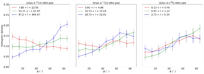
(a)

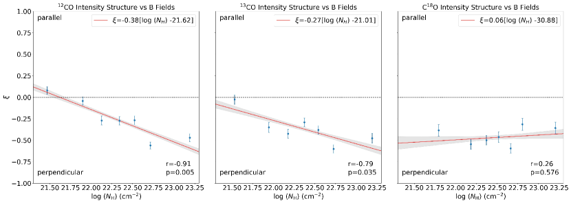
(b)

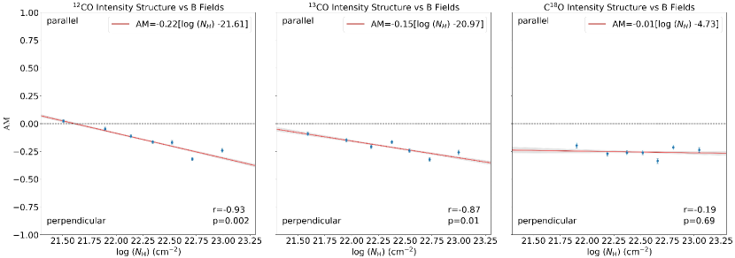
(c)

Figure 4: (a): Histogram of relative orientations between intensity structures for different tracers and magnetic field in the whole Orion A region. The red, green, blue solid lines represent the angle distribution in the lowest, medium, highest intensity bins. (b): Histogram Shape Parameter calculated in different column density bins in the whole Orion A region. The red solid line is the optimal linear fitting results between $\xi$ and column density. The gray area represents the 1$\sigma$ confidence interval of the fitted line. (c): The same as (b), but for the relation between AM and column density.

4 Results

4.1 Results on large scales

We examine the relative orientation between gas intensity structures and the magnetic field across the entire Orion A region at a low resolution ($\sim$ 0.6 pc). The HROs in different intensity bins are presented in Fig. 4(a). The figure illustrates a clear difference in angle distribution among various intensity bins for ¹²CO, ranging from a preference for parallel alignment to a weak preference for perpendicular alignment. This difference becomes less clear with decreasing optical depth of gas tracers. Both $\xi$ and AM exhibits a clear anti-correlation with column densities for ¹²CO and ¹³CO. Regarding C¹⁸O, the orientation between intensity structures and magnetic field prefers to be perpendicular across all column density bins, and there is no correlation between $\xi$/AM and column density. The transition from parallel to perpendicular is consistent with some previous works (Planck Collaboration et al. 2016b; Soler 2019) and MHD simulations (Soler et al. 2013; Chen et al. 2016), indicating a trans-to-sub-Alfvénic state (see Liu et al. 2022 for a review). The variation in results from different gas tracers can be explained by the fact that different gas molecules trace different density regions. In high-density regions, the orientation between intensity structures and the magnetic field is more likely to be perpendicular. The result is consistent with the deduction described in Fissel et al. (2019).

4.2 Results on small scales

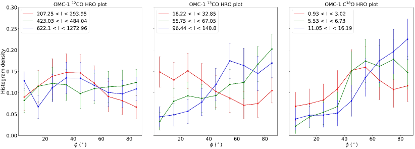
(a)

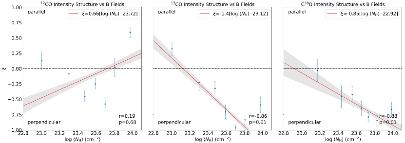
(b)

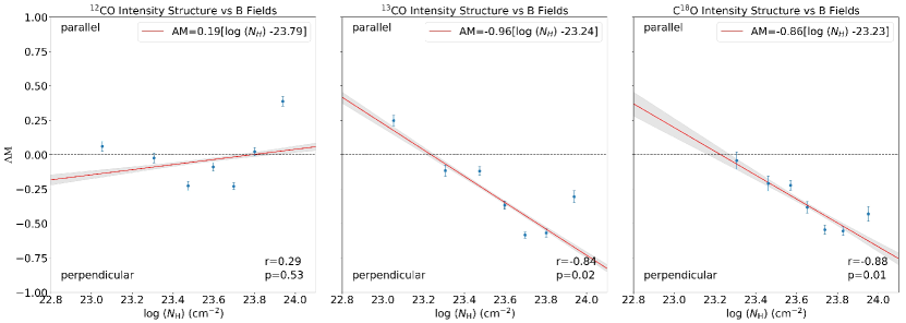
(c)

Figure 5: Same as Fig. 4, but for the relative orientation in OMC-1.

We compare the relative orientation between gas intensity structures and magnetic field in two specific areas (OMC-1, OMC-2/3) within the Orion A region, where high-resolution polarization observations are available ($\sim$ 0.04 pc). There are significantly higher column densities traced in these areas. In this section we present the respective results for each region.

4.2.1 Results in OMC-1

Figure 5(a) illustrates the HRO plots within various intensity bins, while Figs. 5(b) and 5(c) display the correlation between the relative orientation and column densities. In contrast to the findings on large scales, the results in the OMC-1 region differ. We find that the relative orientation between gas intensity structures and magnetic field shows no correlation with column density in the ${}^{12}\mathrm{CO}$ line, but exhibits a clear transition from parallel to perpendicular alignment with increasing column density in the ${}^{13}\mathrm{CO}$ and $\mathrm{C}^{18}\mathrm{O}$ lines. Despite slightly increased uncertainties in calculations due to the limited number of selected pixels, the linear relationship maintains statistical significance after performing Monte Carlo simulations as outlined in Sect. 3.3 ($|r|>0.7,p<0.05$, the $1\sigma$ confidence interval of the best-fit line does not spread much). This phenomenon can be interpreted by the fact that the ${}^{12}\mathrm{CO}$ line is a low-density gas tracer. In the OMC-1 region, ${}^{12}\mathrm{CO}$ is optically thick, and its intensity structure cannot effectively trace the density structure but only the surface of the cloud. On the other hand, the denser gas tracers, ${}^{13}\mathrm{CO}$ and $\mathrm{C}^{18}\mathrm{O}$, prove to be more suitable to trace the density structures.

4.2.2 Results in OMC-2/3

Figure 6(a) presents the HRO plots within various intensity bins, while Figs. 6(b) and 6(c) show the correlation between the relative orientation and column densities now for the OMC-2/3 regions. From the figure, it is evident that there is no statistically significant trend in orientation distribution with increasing column density (all p-values are greater than 0.05). Both $\xi$ and AM are close to 0 across all column density bins, indicating that the relative orientation between intensity structures and the magnetic field is more likely to be randomly distributed in all tracers. We conclude that there is no systematic trend in angle distribution with increasing column densities in the OMC-2/3 region.

A possible explanation for this result is that there are numerous star-forming regions along the long filaments (Chini et al. 1997) and they are at different evolutionary stages (Castets & Langer 1995). The relative alignment between gas structures and the magnetic field is complex in star-forming regions at small scales. The impact of feedback from star-forming activities can lead to the realignment of structures, such as reversing the orientation to parallel via gas flows (Pillai et al. 2020), or inducing a orientation through gravity-dragged rotation (Beuther et al. 2020; Sanhueza et al. 2021). The relative alignment between gas structures and magnetic field in high-mass star-forming regions should be investigated case by case, depending on scales, tracers and evolutionary stages. The results in OMC-2/3 will be discussed further in Sect. 5.1.

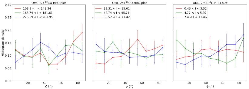
(a)

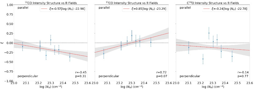
(b)

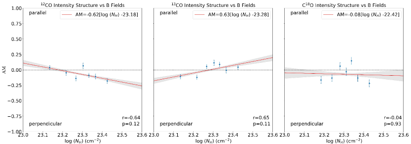
(c)

Figure 6: Same as Fig. 4, but for the relative orientation in OMC-2/3.

5 Discussion

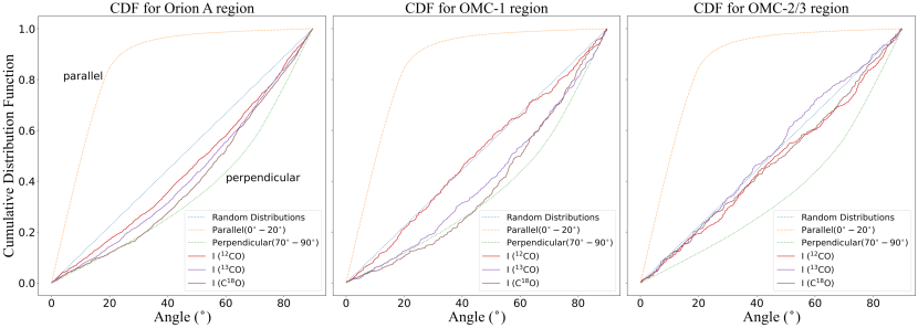
Figure 7: The cumulative distribution functions of relative orientation between intensity structures and magnetic field vectors and the projected $\theta_{3D}$ for Orion A, OMC-1 and OMC-2/3.

5.1 Projection effects

We have measured the relative orientation between intensity structures and magnetic field on the plane of sky. Due to the projection effects, the angle distribution in two dimensions (2D) is not the same with the angle distribution in three-dimensional (3D) space. To examine the projection effects on the measured angle distribution, we carried out a Monte Carol simulation method used in previous study (see Stephens et al. 2017). Here we briefly introduce the method. Firstly we created $10^{6}$ pairs of two random unit vectors within a unit sphere and calculated the angle between the two vectors in 3D space. The angle is within the limit $[0^{\circ},90^{\circ}]$. Then we projected the angle from 3D to 2D space and plot the cumulative distribution functions (CDF) in 2D in three angle bins: (1) purely parallel: angle range from $0^{\circ}$ to $20^{\circ}$ in 3D space, (2) random distribution: angle range from $0^{\circ}$ to $90^{\circ}$ in 3D space and (3) purely perpendicular: angle range from $70^{\circ}$ to $90^{\circ}$ in 3D space. Finally we plot the CDF for our data and compare it with the projected 3D angle.

We present the CDF of $\phi$ and the projected $\theta_{\mathrm{3D}}$ in Fig. 7. In the OMC-2/3 region, a random angle distribution is observed for all tracers. However, in Orion A at a low resolution and the OMC-1 region at a high resolution, a clear transition from random to perpendicular orientation is evident when changing from low-density tracers to high-density tracers, indicating that magnetic fields are dynamically important at both scales. Although the results are influenced by the integration effect along the line of sight, the close-to-perpendicular alignment of the two projected vectors in 2D must also indicate perpendicular alignment in 3D, following the conclusion of previous studies (Planck Collaboration et al. 2016a, b).

The perpendicular alignment can be explained by the contraction scenario of a magnetized, self-gravitating, static collapsing cloud (Mouschovias 1976a, b). On small scales, given that the spatial resolution of polarization observations is comparable to the typical width of filaments (Arzoumanian et al. 2019; André et al. 2022), the filament formation process may affect the magnetic field structures. Earlier studies discussed the relationship between magnetic field orientations and filaments, but no consistent alignment preference was found (Arzoumanian et al. 2021; Baug et al. 2021). In our work, perpendicular alignment is only observed in the OMC-1 region. One possible interpretation is that the magnetic field orientation is almost perpendicular to the major axis of the filament but no similar alignment in the OMC-2/3 region. The gravitational interaction inside the filaments and the BN/KL outflow helps shaping the magnetic field geometry in OMC-1, suggesting feedback from star-forming activities may play an important role on the evolution of magnetic field (Pattle et al. 2017). Another possible explanation is that OMC-1 is at a later evolutionary stage (Castets & Langer 1995). After the long-term evolution, gravitational collapse would be restricted to occur along field lines, and the perpendicular alignment implies that the magnetic field can not efficiently resist gravity (Koch et al. 2018). Compared with OMC-2/3, gravity plays a more important role in OMC-1. The results suggest that perpendicular alignment may only exist in well-evolved, gravity-dominated regions, but observational evidence is still lacking. Further research with larger samples is needed in the future.

5.2 Comparison of HROs with previous studies

We find a similar slope at different scales using HRO analysis. The transition column density, representing the shift from parallel to perpendicular alignment, varies from $10^{21}-4\times 10^{21}\ \mathrm{cm^{-2}}$ on large scales and $8\times 10^{22}-2\times 10^{23}\ \mathrm{cm^{-2}}$ on small scales, depending on the tracers employed. The role pf magnetic field is complex around star-forming regions, with a turning point in $\xi$ and AM (Planck Collaboration et al. 2016b; Ching et al. 2022). After removing the data point of highest column density, the derived transition column density is approximately $4\times 10^{21}\ \mathrm{cm^{-2}}$ at large scales and $1\times 10^{23}\ \mathrm{cm^{-2}}$ at small scales.

Table 1: Summary of HRO analysis

Source	Distance	Resolution	Scale	$X_{\mathrm{HRO}}$	Reference
	(pc)	(′′)	(pc)
Taurus	140	600	0.42	21.84	Planck Collaboration et al. 2016b
Ophiuchus	140	600	0.42	22.70	Planck Collaboration et al. 2016b
Lupus	140	600	0.42	21.72	Planck Collaboration et al. 2016b
Chamaeleon-Musca	160	600	0.48	21.67	Planck Collaboration et al. 2016b
Corona Australia (CrA)	170	600	0.51	24.14	Planck Collaboration et al. 2016b
Aquila Rift	260	600	0.78	22.23	Planck Collaboration et al. 2016b
Perseus	300	600	0.90	21.76	Planck Collaboration et al. 2016b
IC5146	400	600	1.20	21.79	Planck Collaboration et al. 2016b
Cepheus	440	600	1.32	21.90	Planck Collaboration et al. 2016b
Orion	450	600	1.35	21.88	Planck Collaboration et al. 2016b
Vela C-South-Nest	933	180	0.84	22.23	Soler et al. 2017
Vela C-South-Ridge	933	180	0.84	22.40	Soler et al. 2017
Vela C-Centre-Nest	933	180	0.84	22.62	Soler et al. 2017
Vela C-Centre-Ridge	933	180	0.84	20.69	Soler et al. 2017
DR21	1400	14	0.10	21.20	Ching et al. 2022
Serpens Main	415	14	0.03	—–	Kwon et al. 2022
OrionA	414	300	0.62	20.97-21.62	this work
OMC-1	414	20	0.04	22.92-23.24	this work
OMC-2/3	414	20	0.04	—–	this work

Planck Collaboration et al. (2016b) investigated the HROs in ten nearby clouds (d $<$ 450 pc) with a resolution of $10^{\prime}$. They find a common transition from parallel to perpendicular with increasing column densities, and the typical transition column density is approximately $5\times 10^{21}\ \mathrm{cm^{-2}}$. Soler et al. (2017) adopted the HRO analysis in Vela C region (d $\sim$ 933 pc) with a resolution of $3^{\prime}$ using BLASTPol balloon-borne telescope. The similar trend is found and the transition column density ranges from $5\times 10^{21}$ to $2\times 10^{23}\ \mathrm{cm^{-2}}$.

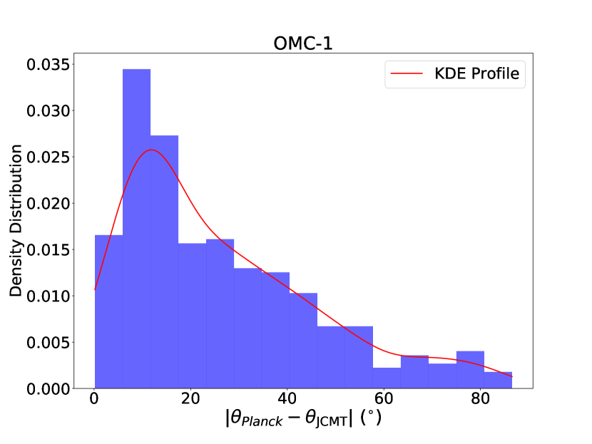
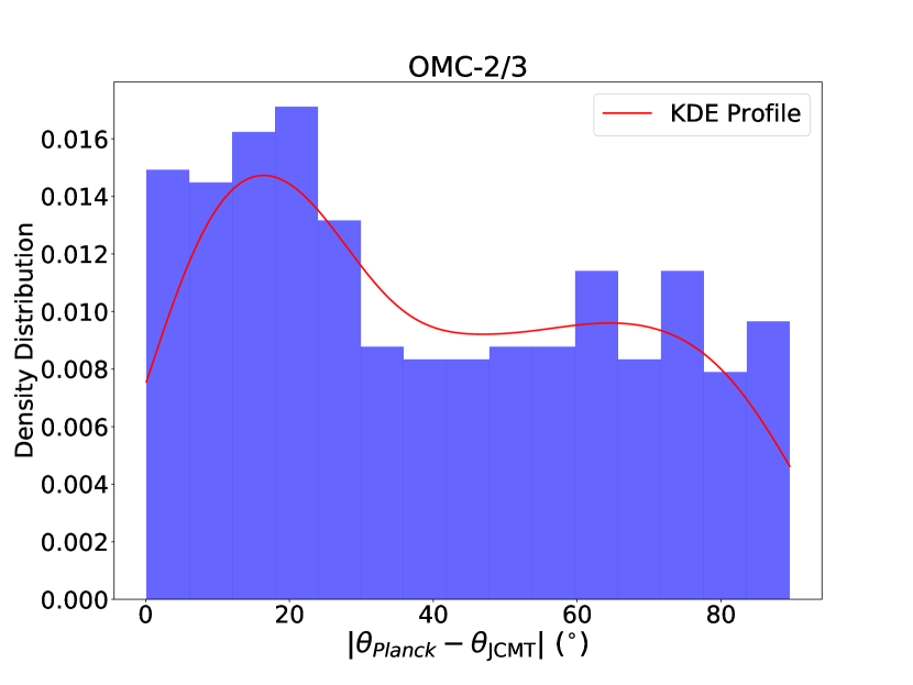
Figure 8: The histogram of relative orientation between Planck and JCMT derived magnetic field in OMC-1 and OMC-2/3. The red line represents the Gaussian kernel density estimate of the angle difference.

On small scales, Ching et al. (2022) applied the HRO analysis toward the DR21 filament (d $\sim$ 1.4 kpc) using JCMT with a resolution of $14^{\prime\prime}$ and the resulting transition column density is $1.6\times 10^{21}\ \mathrm{cm^{-2}}$. Kwon et al. (2022) investigated the HRO of the Serpens Main region (d $\sim$ 415 pc) using JCMT with a resolution of $14^{\prime\prime}$. They find a complex relationship between $\xi$ and column density, featuring several turning points and no clear transition column density. The detailed information of all the HRO analysis is summerized in Table 1.

Considering all the findings, a consistent trend from parallel to perpendicular alignment with increasing column densities is observed in most regions. However, the transition column density is scale-, tracer-, and environment-dependent. We do not find a uniform transition column density, suggesting that the HRO analysis should be applied case-by-case. We note that it is a comparison between single region studies (this work, Soler et al. 2017, Ching et al. 2022, Kwon et al. 2022) and statistical studies (Planck Collaboration et al. 2016b). The conclusion from case studies can not be directly utilized in other star-forming regions.

The variation in relative orientation among different gas tracers is also interesting. Fissel et al. (2019) report no changes in relative orientation with increasing column densities across all tracers. However, they observe a transition from parallel to perpendicular alignment when changing from low-density tracers to high-density tracers. Using a three-dimensional, turbulent collapsing-cloud MHD simulation, Mazzei et al. (2023) compared relative alignment between magnetic fields and molecular gas structure across different tracers. They find good agreement between their simulations and the results obtained in Fissel et al. (2019). However, They suggest ¹²CO would remain in parallel alignment across the whole observer space, which is in contrast with our results. In our analysis, we have not only observed the variation of relative orientation with different gas tracers but also identified its changes with column density at different scales. This implies that the physical processes in the Orion A molecular cloud are hierarchical and highly complicated, making them challenging to be explained by the simulations.

5.3 The relative orientation between Planck- and JCMT- derived magnetic field

Another interesting question to explore is the relative orientation between magnetic fields at different scales. Zhang et al. (2014) first investigated this question, comparing SMA and parsec-scale magnetic fields and discovering a bimodal orientation distribution. They suggested that the magnetic field at the core scale could align either parallel or perpendicular to that of the clump scale. Li et al. (2015) revealed that the magnetic field directions do not change much from cloud to clump and core scales in NGC 6334. In our study, we interpolate the Planck data and calculate the magnetic field orientation at large scales using the transformation in Sect. 2.1, and then compute the angular difference in specific regions.

Figure 8 illustrates the distribution of angle differences between large-scale and small-scale magnetic fields. We use the Gaussian kernel density estimate (KDE) to represent the probability density function of the angle difference. In the OMC-1 region, small-scale magnetic fields align well with Planck data, with 79$\%$ of them having an angle difference within 40 degrees of the large-scale magnetic fields. Regarding the OMC-2/3 region, the angle difference shows a broader distribution. This region exhibits a bimodal orientation distribution, similar to findings reported by Zhang et al. (2014), with 59$\%$ of them displaying an angle difference within 40 degrees. The discrepancy in alignment between large-scale and small-scale magnetic fields could be attributed to the impact of foreground dust emission from Planck observations, as suggested by Gu & Li (2019). A more important factor is the geometry of small-scale magnetic fields. As discussed in Zhang et al. (2014), a random orientation of fields would lead to a uniform distribution of angle differences. As the magnetic field properties vary rapidly in different sub-regions of OMC-2/3 (Poidevin et al. 2010), the orientation distribution is much flatter than that in OMC-1. Whether star-forming activities affect the alignment of magnetic fields at different scales needs further discussion in a larger sample with well-ordered magnetic field geometry in the future.

6 Summary

We compare the gas intensity structures of three gas tracers (¹²CO, ¹³CO and C¹⁸O) with magnetic fields at different scales. We apply the HRO technique in our analysis to examine the relation between the relative orientation of gas structures with respect to magnetic fields and column densities. Our main findings are as follows:

1. We find a similar trend in relative orientation between magnetic field and molecular gas intensity structures with respect to column densities at different scales in Orion A. Through a comparison with previous studies, we find the trend is common in molecular clouds at pc scales but not uniform at $<$ 0.1 pc scales. The relation between gas structures and magnetic field should be discussed case by case in individual star-forming regions at small scales.

2. When the orientation is not randomly distributed, we see a significant change in the relative orientation distribution between gas intensity structures and magnetic fields for three different molecular gas tracers. The perpendicular alignment is more clear when changing from low-density tracers to high-density tracers. The correlation between gas intensity structures and magnetic field is better traced by low-density gas tracers on large scales and high-density tracers on small scales, indicating the different roles of magnetic field in cloud formation and filament formation. The results found in this work only applies to Orion A region and can not be directly extrapolated for other star-forming regions.