Cooper pairing, flat-band superconductivity and quantum geometry
in the pyrochlore-Hubbard model
Abstract
We investigate the impacts of the quantum geometry of Bloch states, specifically through the band-resolved quantum-metric tensor, on Cooper pairing and flat-band superconductivity in a three-dimensional pyrochlore-Hubbard model. First we analyze the low-lying two-body spectrum exactly, and show that the pairing order parameter is uniform in this four-band lattice. This allowed us to establish direct relations between the superfluid weight of a multiband superconductor and () the effective mass of the lowest-lying two-body branch at zero temperature, () the kinetic coefficient of the Ginzburg-Landau theory in proximity to the critical temperature, and () the velocity of the low-energy Goldstone modes at zero temperature. Furthermore, we perform a comprehensive numerical analysis of the superfluid weight and Goldstone modes, exploring both their conventional and geometric components at zero temperature.
I Introduction
The complex quantum geometric tensor serves as a central and defining concept in modern solid-state and condensed-matter physics [1, 2, 3]. Its imaginary component is in the form of an anti-symmetric tensor known as the Berry curvature, and the associated Chern number has proven instrumental in the classification of topological insulators and superconductors [4, 5, 6, 7]. Its real part is in the form of a symmetric tensor known as the quantum metric, and it quantifies the quantum distance between adjacent Bloch states. Despite a long history of interdisciplinary interest in various physical phenomena governed by the Berry curvature, nature has been less forthcoming regarding the effects of the quantum metric. Only in the past decade or so have researchers increasingly recognized the significance of the quantum metric in various contexts. Notably, following the pioneering work by Peotta and Törmä in 2015 on the origins of superfluidity in topologically-nontrivial flat bands [8], a deeper connection between the transport properties of a multiband superconductor and the quantum geometry of its Bloch states has emerged as a surprising revelation in recent years [9, 10, 11, 12, 13, 14].
Theoretical interest in flat-band superconductivity dates back a long time, as materials hosting quasi-flat Bloch bands were envisioned as a potential pathway to achieve room-temperature superconductivity [15, 16]. This anticipation was grounded in the naive BCS theory, which was suggested by the relatively elevated single-particle density of states within narrower Bloch bands. However, it is crucial to emphasize that the microscopic mechanism underpinning the emergence of flat-band superconductivity was completely absent in these earlier studies. It remained unclear whether superconductivity could thrive within an isolated flat band, given that the infinite effective band mass hampers the potential for localized particles on the lattice to attain superconductivity, thus acting as an inhibiting factor. As a result, it was believed that superconductivity was strictly prohibited when the permissible Bloch states originated solely from a single flat band [17].
Recent studies illuminated these two perplexing arguments and unveiled a physical mechanism that theoretically permits the existence of flat-band superconductors [9, 10, 11]. It has been demonstrated that multiband lattices (such as in Moiré materials) contribute differently to the superfluid weight. The real intraband processes were associated with the conventional contribution, while the virtual interband processes were linked to the geometric aspect. Unlike the conventional contribution [18, 19], which is solely determined by the derivatives of the Bloch bands, the geometric contribution is also influenced by the derivatives of the associated Bloch states. Consequently, unless the geometric contribution is nullified, superconductivity can manifest within a flat band, thanks to the involvement of other flat or dispersive bands through interband processes.
These findings highlight the necessity of considering not only the dispersion of the Bloch bands but also the geometry of the Bloch states in the pursuit of high-critical-temperature superconductivity. It is only by incorporating both factors that we can fully exploit their potential. A non-trivial quantum geometry is indispensable, as the mere presence of a flat band does not guarantee superconductivity if its geometry is trivial. Thus, the emerging field of quantum geometry within multiband superconductors holds substantial potential for advancing our understanding of flat-band superconductors, assuming Hubbard-type tight-binding Hamiltonians mimic their underlying low-energy physics. Despite the significant progress made with one-dimensional and two-dimensional lattices that feature flat bands [20, 21, 22, 23, 24, 9, 10, 25, 26, 27, 28, 29, 30, 31], there has been limited exploration of more realistic three-dimensional lattices due to the technical complexities and challenges associated with their analysis. Our aim is to fill this gap by investigating quantum-geometric effects in a pyrochlore-Hubbard model, where the pyrochlore lattice consists of a three-dimensional arrangement of tetrahedra sharing corners, possesses cubic symmetry, and is commonly encountered in transition-metal and rare-earth oxide materials, especially in oxide compounds [32]. Given the recent demonstrations of three-dimensional flat bands and superconductivity in a pyrochlore metal CaNi2 [33] and pyrochlore superconductor CeRu2 [34], these structures present a compelling lattice platform for exploring the interplay between quantum geometry and strong correlations.
The rest of the paper is organized as follows. In Sec. II we introduce the pyrochlore lattice, and discuss its one-body spectrum. In Sec. III we calculate the low-lying two-body spectrum for the pyrochlore-Hubbard model, and derive the effective mass tensor of the lowest-lying branch. In Sec. IV we analyze the superfluid weight at zero and finite temperatures, relate it to the velocity of the low-energy Goldstone modes at zero temperature, and present their thorough numerical exploration in Sec. V. The paper ends with a summary and an outlook in Sec. VI, and the Gaussian fluctuations are discussed in Appendix A.
II One-body problem
The pyrochlore lattice is one of the simplest three-dimensional tight-binding models that feature a flat band in the Bloch spectrum [35, 36]. It has an underlying face-centered-cubic Bravais lattice that can be defined by the primitive unit vectors , and , where is the side-length of the conventional simple-cubic cell. Its basis consists of sublattice sites that are located at , , and . The corresponding first Brillouin Zone (BZ) has the shape of a truncated octahedron with a side-length . The associated reciprocal space is such that where is the crystal momentum in units of and is the number of unit cells in the system. That is the total volume of the system is , where is the volume of the BZ in reciprocal space, is the volume of the primitive cell in real space, and is the total number of lattice sites in the system.
Having a spin- system in mind with labeling the spin projections, the Bloch Hamiltonian for such a lattice can be written as where annihilates a spin- particle on the sublattice with momentum . The elements of the Hamiltonian matrix are real such that and where is the hopping parameter between the nearest-neighbor sites. Thus respects time-reversal symmetry. The resultant eigenvalue problem, i.e.,
| (1) |
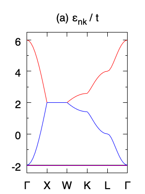
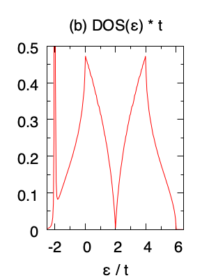
leads to four Bloch bands in the one-body spectrum, where and are the dispersive bands with and are the flat bands. These bands are sketched in Fig. 1(a) along the high-symmetry points. In this paper, since we prefer the flat bands to appear at the bottom of the spectrum, we set and choose as the unit of energy.
In Fig. 1(b), we also show the single-particle density of states per unit cell per spin where the Dirac-delta function is represented via a Lorentzian distribution with . This is the origin of the energy broadening around . The van Hove singularities are clearly visible at , and the density of states vanishes linearly at with logarithmic corrections in its vicinity. The total bandwidth is .
III Two-body problem
In this paper we consider the simplest Hubbard model with an onsite attractive interaction between an and a particle,
| (2) |
where . The two-body problem can be solved exactly through a variational approach [37], leading to a number of bound states for a given center-of-mass momentum . It turns out the low-lying two-body spectrum can be determined by where is a Hermitian matrix with the following elements
| (3) |
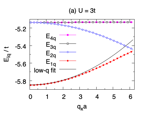
Here we assumed time-reversal symmetry and where is the sublattice projection of the periodic part of the Bloch state that is associated with through Eq. (1). This yields a self-consistency relation for a given , and its solutions can be found by setting the eigenvalues of to one at a time. The corresponding eigenvectors can be used to characterize some physical properties of the bound states, where is the transpose. Thus, for a given , there are 4 bound states below the threshold of the lowest two-body continuum, and we label them with starting with the lowest branch. These solutions are illustrated in Fig. 2(a) for , where the degenerate branches appear almost flat in the shown scale since their bandwidths are roughly . The overall structure of the two-body spectrum is reminiscent of the underlying Bloch spectrum but with the opposite sign of energy. Compare with the - portion in Fig. 1(a). This can be best understood in the , where the effective nearest-neighbor hopping parameter for a strongly-bound pair of and particles has the opposite sign compared to of its unpaired constituents. This is because when a bound state breaks up at a cost of binding energy in the denominator and its constituent hops to a neighboring site, the partner follows it and hops to the same site, leading to in the numerator. The prefactor accounts for the possibility of change in the order of spins. Such a virtual dissociation is the only physical mechanism for a strongly-bound pair of particles to move in the Hubbard model with nearest-neighbor hoppings.
Our numerical calculations also reveal that the so-called uniform-pairing condition [37], i.e., is satisfied at all for the lowest-lying branch in the limit. This finding suggests that the sublattice sites of a pyrochlore lattice in a unit cell must be equivalent by symmetry and make equal contribution to pairing. Thus, similar to the well-known two-dimensional toy models such as Mielke-checkerboard and kagome lattices that exhibit uniform pairing, the pyrochlore lattice offers an ideal playground for theoretical studies on flat-band superconductivity in three dimensions. For instance, when the uniform-pairing condition is met together with the underlying time-reversal symmetry, the energy of the corresponding small- bound states can be extracted simply from . In particular, it is possible to show that [37]
| (4) |
where the energy offset is determined by the self-consistency relation [37]
| (5) |
Furthermore, we split the elements of the inverse effective-mass tensor as depending on whether the intraband or interband processes are involved, leading to [37]
| (6) | ||||
| (7) |
Here the intraband contribution depends only on the derivatives of the Bloch spectrum but the interband contribution depends also on the derivatives of the associated Bloch states through the elements of the so-called band-resolved quantum-metric tensor
| (8) |
where denotes the real part and As the naming suggests, the elements of the quantum-metric tensor of the th Bloch band [3] can be written as Their origin can be traced back to the power-series expansion of in powers of .
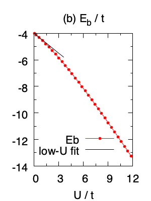
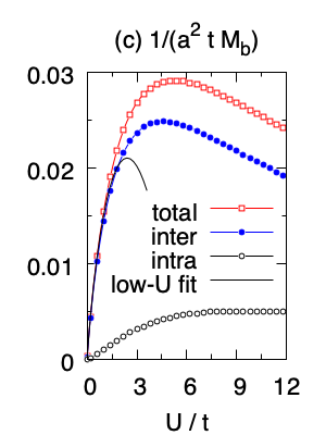
In Figs. 2(b) and 2(c), we present the self-consistent solutions of Eqs. (5), (6) and (7) for the pyrochlore lattice, where the effective mass is isotropic in space. As an illustration, we show in Fig. 2(a) that the resultant and provide a perfect fit when . Furthermore, in the limit when , one can make analytical arguments that are based on some controlled approximations that to the leading order, where and are numerical factors and . Our numerical fit for shows that , and . This fit is shown in Fig. 2(c), and it works quite well up to . Similarly, in the limit when , one can show that where is the effective hopping parameter for a strongly-bound pair as discussed above. For instance when . We also note that this finding is consistent with the effective-mass tensor of the highest Bloch band where
IV Many-body Problem
Given that the uniform-pairing condition is satisfied for the lowest-lying two-body bound states when , the analogous Cooper pairing and its many-body BCS mean-field extension (i.e., assuming stationary Cooper pairs with zero center-of-mass momentum) are also described by a uniform order parameter in a unit cell.
IV.1 BCS-BEC crossover
For this reason, we take as the uniform order parameter for superconductivity in all four sublattices, and set it to a real positive number. Following the standard prescription, we obtain the mean-field self-consistency relations [22]
| (9) | ||||
| (10) |
where is a thermal factor with the Boltzmann constant and the temperature, is the shifted dispersion with the chemical potential, is the intraband quasiparticle spectrum, and the particle filling corresponds to the total number of particles per site. Note that there is no interband pairing since the underlying time-reversal symmetry guarantees the presence of a particle in Bloch state for every particle in , as the energetically most favorable BCS scenario for the stationary pairs. Self-consistent solutions of Eqs. (9) and (10) for and is the starting point of the BCS-BEC crossover theories, and they are known to produce qualitatively correct results at sufficiently low including the limit. In addition the mean-field expression for the filling of condensed particles [22, 38]
| (11) |
plays an important role in our discussion below, and it also produces qualitatively correct results at all as long as is sufficiently low.
IV.2 Superfluid weight
When the uniform-pairing condition is met together with the time-reversal symmetry, the superfluid phase-stifness tensor or often called the superfluid weight can be written as depending on whether the intraband or interband processes are involved. Using a linear-response theory and Kubo formalism or simply by imposing a phase-twist in the order parameter [21, 22, 39], it can be shown that
| (12) | ||||
| (13) |
where is another thermal factor. Thus, similar to the inverse effective-mass tensor of the lowest-lying two-body branch, the intraband contribution depends only on the derivatives of the Bloch spectrum but the interband contribution depends also on the band-resolved quantum-metric tensor. For this reason the former (latter) is also referred to as the conventional (geometric) contribution, where Eq. (12) can also be put in the more familiar form, i.e., after some integration by parts and algebra, from the well-known single-band case [22, 19]. Next we show that the geometric origin of the superfluid weight can be traced all the way back to the effective mass of the superfluid carriers.
IV.2.1 limit
Lets first analyze Eqs. (12) and (13) at . Assuming , we may set and leading to
| (14) |
where is the derivative of the Hamiltonian matrix. Here we concentrate on two physically transparent limits. The first one is the limit, where and such that For this reason, we may set in Eq. (14), and calculate leading eventually to where and is a Kronecker delta. This result can be understood as follows. In the case of a continuum model with a single parabolic dispersion and an attractive -wave contact interaction between particles, it can be shown that , where is the superfluid density. When these particles form strongly-bound weakly-interacting pairs in the BEC limit, we may set as the superfluid density of pairs and as their mass, leading to in terms of the pair properties [22, 23]. Furthermore, given that all of the particles participate in the superfluid flow at for any interaction strength in a continuum model, i.e., where is the filling of superfluid particles in the corresponding lattice model, we expect where is the filling of superfluid pairs. Moreover, substituting as in the limit, we identify as the effective mass of the superfluid pairs in a pyrochlore lattice. It is pleasing to see that this analysis is in full agreement with of the effective band-mass of the lowest-lying two-body branch.
The second limit is the extremely-low particle-filling case and its extremely-high particle-filling counterpart (which is equivalently to the extremely-low hole-filling), where and in the former, and and in the latter with for any . For this reason we may set and obtain
| (15) | ||||
| (16) |
where we used integration by parts in Eq. (15), and and in the evaluation of Eq. (16). In addition, using the density of superfluid pairs along with we eventually find
| (17) |
for the limit, where is precisely the inverse effective mass tensor of the lowest-lying two-particle bound states given by Eqs. (6) and (7) after setting and Note that limit is similar but with the appearance of inverse effective mass tensor of the highest-lying two-hole branch.
IV.2.2 limit
Lets also analyze Eqs. (12) and (13) in the vicinity of the critical superconducting transition temperature . Since in the limit from below, we may set and obtain
| (18) | ||||
| (19) |
where and Here we used integration by parts that is followed by another integration by parts in Eq. (18), and and in the evaluation of Eq. (19). Note that Eqs. (18) and (19) reproduce, respectively, Eqs. (15) and (16) in the limit when , e.g., in the where . It is pleasing to see that
| (20) |
where is precisely the kinetic coefficient that appears in the Ginzburg-Landau theory near [40], determining not only the superfluid density and effective mass of the superfluid carriers but also the coherence length, magnetic penetration depth, upper critical magnetic field, etc. Notably, certain among these quantities have already been measured to characterize geometric effects in twisted bilayer graphene [41].
IV.3 Low-lying Goldstone modes at
Similar to the superfluid weight, next we show that the low-energy collective modes also have a quantum-geometric origin [42]. As discussed in the Appendix A, the dispersion for the collective Goldstone modes is determined by the poles of the fluctuation propagator , i.e., by setting , after an analytic continuation to the real axis. At , the matrix elements of reduce to
| (21) | ||||
| (22) | ||||
| (23) |
where we denote by , by , by and by . To determine the lowest-energy Goldstone modes, it is sufficient to retain terms up to quadratic order in their small and expansions, leading to and In the expansion of , the zeroth-order term vanishes due to the saddle-point condition given in Eq. (9). The non-kinetic expansion coefficients and are simply given by a sum of their single-band counterparts. When , it is clearly seen that the phase and amplitude modes are decoupled, and this is known to be the case only in the strict BCS limit [43].
Similar to the superfluid weight, the kinetic coefficients can be written as and depending on whether the intraband or interband processes are involved, leading to
| (24) | ||||
| (25) | ||||
| (26) | ||||
| (27) |
Using some integration by parts and algebra, the intraband coefficients can also be put in the more familiar forms, and from the well-known single-band case [42, 43] 111 In the case of two-band lattices, our expansion coefficients recover all of the previous results except for the first line of Eq. (27), which is missing there [42]. . By setting , we obtain
| (28) |
which is the dispersion for the low-momentum and low-frequency Goldstone modes. Thus, at , we are pleased to verify that the low-energy collective excitations have a linear dispersion whose finite velocity is characterized by the superfluid weight, i.e.,
| (29) |
which is in accordance with the Landau’s criterion for superfluidity.
V Numerical Results
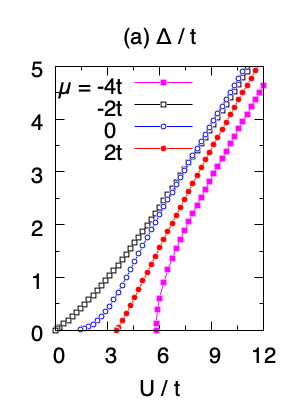
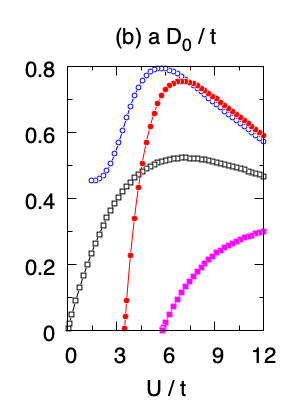
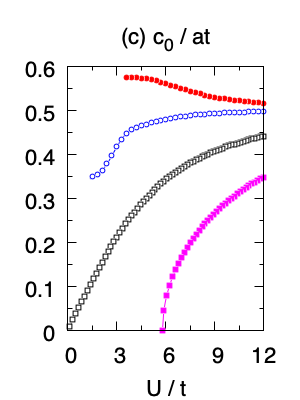
In this section we exclusively set , and determine and self-consistently from Eqs. (9) and (10), and then plug them into Eqs. (12) and (13) as a function of . Typical solutions are shown in Fig. 3. When particle filling lies within the flat bands, i.e., when or equivalently at , it can be shown that [45] and in the limit. Note that these expressions are quite similar to those of the limit’s results, because, given that with being the bandwidth of a flat band, even an arbitrarily small but finite corresponds effectively to a strong-coupling limit. Accordingly, when coincides perfectly with a flat band at (or equivalently corresponds to , i.e., to a half-filled flat bands), grows linearly with as shown in Fig. 3(a). In this case our numerical fit for shows that , and , and this fit works very well up to . This finding is in sharp contrast with the recent results on two-dimensional lattices, where a band touching with a flat band causes logarithmic corrections to the linear in term that is expected for an energetically-isolated flat band in any dimension [23, 24]. It is pleasing to see that this fit is quite similar in structure to of the two-body problem, where . The ratios and are not expected to be similar unless .
It can also be shown that, while the BCS order parameter grows exponentially slow when and lies within any of the dispersive Bloch bands, it grows linearly fast from the critical semi-metal point with when or equivalently , and with a square root from the particle and hole vacuums when or . For instance when . These are illustrated in Fig. 3(a). The corresponding are shown in Fig. 3(b), where it saturates at sufficiently small when lies within any of the dispersive Bloch bands, and vanishes otherwise.
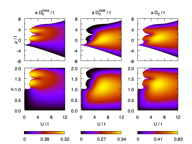
In Fig. 4 we present maps of the superfluid weight together with its and contributions as a function of , and . Due to technical difficulties, i.e., the accuracy of the numerical integration becomes unreliable when the exponential growth of is not accurately captured by the non-linear solver due to the convergence problems, we choose to present the data in the parameter regime where . This is why Fig. 4 has white regions, e.g., in the lower panels, even though corresponds to a partially-filled dispersive Bloch band in the limit where is known to saturate. This drawback offers the advantage that the single-particle density of states shown in Fig. 1(b) appears on the periphery of the white regions, including the flat bands at , van Hove singularities at or equivalently at , and the critical semi-metal point at or equivalently at . On the other hand, the peripheries of the particle and hole vacuums and the critical semi-metal point are determined quite accurately in the upper panels, since vanishes very rapidly in their vicinity when , e.g., see Fig. 3(a). This is also indicated by the nearly invisible white regions at the edges of the lower panels when or .
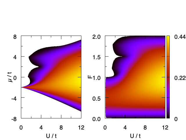
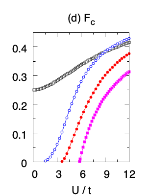
In the small regime, Fig. 4 clearly shows that while is the dominant contributor in the flat-band superconductivity, i.e., when , dominates the usual superconductivity in general when lies within a dispersive band. However, both contributions are equally important in the large regime including the limit (not shown). In fact even at . We checked that the total superfluid weight approaches in the limit, which is in perfect agreement with the analysis given in Sec. IV.2.1. Since the filling of condensed particles plays a critical role in connecting to the effective mass of the superfluid carriers, we also present its map in Fig. 5 as a function of , and . This figure verifies that (derived above) saturates when in the limit as soon as , and that all of the particles are entirely condensed in a dilute flat-band superconductor, i.e., when in Fig. 5. Such a perfect condensation may occur only if the repulsive interaction between small Cooper pairs is negligible, which may be the underlying reason behind our finding in Sec. IV.2.1 that is determined entirely by the effective mass of the lowest-lying two-body branch when . This is in sharp contrast with the usual superconductors where corresponds to a negligible fraction of particles in the small regime, which can also be seen in the region in Fig. 5. We again checked that in the limit, which is in perfect agreement with the analysis given in Sec. IV.2.1.
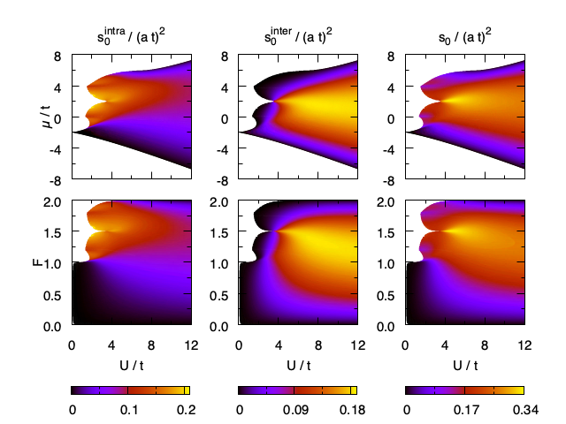
In Fig. 6 we present maps of the square of the isotropic sound speed together with its and contributions as a function of , and . First of all, both and saturate in the limit when lies within a dispersive band and is small and negligible. These are expected from the well-known single-band results [46]. In addition, for a fixed in the small regime, both and exhibit faint but visible dips around the van Hove singularities, which are also consistent with the well-known single-band results [46]. On the other hand, when coincides perfectly with a flat band at , both and grow from with a power-law (approximately quadratically) in but remain small and negligible. Thus, vanishes linearly with in a flat-band superconductor in the limit, which is in sharp contrast with the usual dispersive case where it saturates. In order to characterize and understand this particular limit, we set for the flat bands and take only their contributions into account, leading to , and , where . Furthermore, using the relation we find , which is in perfect agreement with the numerics. In addition, at the semi-metal critical point when and , both and exhibit comparable jumps from . Because of this, the resultant exhibits a much larger jump right at the tip of the critical region, since is typically small and negligible in its vicinity. Lastly we consider the limit, and set for all bands, leading to , , and . The resultant depends only on as in the case of single-band case [46], and it is in perfect agreement with the numerics. It can be written in a form that is identical to the flat-band expression above. We also find it instructive to reinterpret the sound speeed in terms of the filling and effective mass of the pairs. Then, by making a comparison with the Bogoliubov expression that is valid for a weakly-interacting Bose gas on a tight-binding lattice [47], we identify as the parameter that characterizes the interaction between pairs in the limit. Such a strong and repulsive onsite interaction between pairs of fermions can be attributed to the underlying Pauli exclusion principle [46]. On a similar footing, using the results of Sec. IV.2.1 where for a dilute () flat-band superconductor when , we also reach the conclusion that . This suggests that the interaction between pairs tends to zero in a flat-band superconductor.
VI Conclusion
To summarize, we studied the impact of the quantum geometry of Bloch states, specifically through the band-resolved quantum-metric tensor, on Cooper pairing and flat-band superconductivity within a three-dimensional pyrochlore-Hubbard model. For this purpose, first we showed that the pairing order parameter is uniform in this four-band lattice through an exact calculation of the low-lying two-body spectrum. This simplification enabled us to reveal direct relations between the superfluid weight of a multiband superconductor and () the effective mass of the lowest-lying two-body branch at through () the kinetic coefficient of the Ginzburg-Landau theory near through and () the velocity of the low-energy Goldstone modes at through The underlying physics behind these relations is that a bound state with a finite center-of-mass momentum is a collective mode of the superfluid ground state. Then we presented a thorough numerical analysis of the superfluid weight and Goldstone modes together with their intraband (conventional) and interband (geometric) contributions at zero temperature. For instance, one of our important observations is that, in sharp contrast with the recent results on two-dimensional lattices where a band touching with a flat band causes logarithmic corrections to the superfluid weight in the limit, the analogous correction is a power law in three dimensions which may be approximated by Another one is the relation between the sound speed and the superfluid weight in a flat-band superconductor when which further suggests that the the interaction between pairs tends to zero.
Much like the well-explored two-dimensional toy models such as Mielke-checkerboard and kagome lattices, which display uniform pairing, we believe the pyrochlore lattice presents an excellent setting for conducting theoretical research on three-dimensional flat-band superconductivity. As an outlook we are planning to develop a Ginzburg-Landau theory for the pyrochlore-Hubbard model, and explore how quantum geometry effects not only the superfluid density and effective mass of the superfluid carriers but also the coherence length, magnetic penetration depth, upper critical magnetic field, etc in the BCS-BEC crossover [40].
Acknowledgements.
The author acknowledges funding from US Air Force Office of Scientific Research (AFOSR) Grant No. FA8655-24-1-7391.Appendix A Gaussian Fluctuations
In order to go beyond the saddle-point (mean-field) approximation, we use imaginary-time functional path-integral formalism [42, 43] and derive a quadratic effective action in the fluctuations of the order parameter for a multiband Hubbard model with onsite attraction. It turns out this formalism is drastically simpler and transparent when the system manifests both time-reversal symmetry and uniform-pairing condition as in pyrochlore lattice of interest. In this case the bosonic Hubbard-Stratavonich field (which plays the role of the order parameter) can be split as
| (30) |
for all sublattice sites in a unit cell, where the complex field corresponds to the fluctuations around the stationary saddle-point parameter (which is taken as real here and in the main text), and is a collective index with the bosonic Matsubara frequency. Given our interest in the low-energy in-phase (i.e., Goldstone) collective modes only, we also set to be uniform together with , making higher-energy out-of-phase (i.e., Leggett) collective modes inaccessible. The latter can be studied through an -dependent , which is beyond the scope of this paper.
First we express the mean-field Hamiltonian in the Bloch-band representation, whose Hamiltonian matrix can be expressed as
| (31) |
where and are Pauli matrices describing the particle-hole degrees of freedoms. Then the saddle-point propagator can be written as where is a combined index with the fermionic Matsubara frequency. Here defines the quasiparticle-quasihole spectra with , where the associated eigenvectors are for the quasiparticles and for the quasiholes. The coherence factors and coincide with the usual intraband expressions due to the absence of interband pairing.
Following the standard procedure, the quadratic effective action can be written as where denotes a trace over the band and particle-hole sectors, and is controlled purely by the fluctuation fields. Here is the number of sublattices in a unit cell (which is 4 for the pyrochlore lattice), and is an unit matrix in the band space. Upon evaluation of the trace and sum over the fermionic frequencies, we eventually obtain
| (36) |
where the fluctuation matrix plays the role of inverse-propagator of amplitude and phase fluctuations. In order to express its matrix elements in a compact form, we denote by , by , by , by , and denote their functions as , , , , and , leading to
| (37) | ||||
| (38) |
Note that while is even both under and , is even only under . In the presence of a single band, these expressions recover the usual results [42, 43].
Next we introduce a unitary transformation and associate and with the amplitude and phase degrees of freedom, respectively. Assuming these are real functions in real space and time, we set and , and express the effective action in the form
| (43) |
where is an even function of and is an odd one. In particular when , since the off-diagonal terms necessarily vanish, we observe that the amplitude and phase modes are always decoupled in the low-momentum and low-frequency limit. Furthermore the fact that vanish, due to the saddle-point condition, (i.e., the order parameter Eq. (9)), suggests that the low-frequency phase mode is always gapless, and we identify it as the Goldstone mode. Similarly, when , the fact that vanish, due again to the saddle-point condition, suggests that the amplitude mode is gapped with , and we identify it as the Higgs mode. Note that, since does not vanish in general, the latter statement is strictly valid only in the BCS limit where is small and negligible.
Given that the terms with the prefactor have the usual Landau singularity for limit and causes the collective modes to decay, a small expansion is well-defined only in two cases: () just below as discussed in Ref. [40], and () at which is discussed in the main text.
References
- Provost and Vallee [1980] J. P. Provost and G. Vallee, Riemannian structure on manifolds of quantum states, Commun. Math. Phys. 76, 289 (1980).
- Berry [1984] M. V. Berry, Quantal phase factors accompanying adiabatic changes, Proceedings of the Royal Society of London. A. Mathematical and Physical Sciences 392, 45 (1984).
- Resta [2011] R. Resta, The insulating state of matter: a geometrical theory, The European Physical Journal B 79, 121 (2011).
- Xiao et al. [2010] D. Xiao, M.-C. Chang, and Q. Niu, Berry phase effects on electronic properties, Rev. Mod. Phys. 82, 1959 (2010).
- Qi and Zhang [2011] X.-L. Qi and S.-C. Zhang, Topological insulators and superconductors, Rev. Mod. Phys. 83, 1057 (2011).
- Chiu et al. [2016] C.-K. Chiu, J. C. Y. Teo, A. P. Schnyder, and S. Ryu, Classification of topological quantum matter with symmetries, Rev. Mod. Phys. 88, 035005 (2016).
- Bansil et al. [2016] A. Bansil, H. Lin, and T. Das, Colloquium: Topological band theory, Rev. Mod. Phys. 88, 021004 (2016).
- Peotta and Törmä [2015] S. Peotta and P. Törmä, Superfluidity in topologically nontrivial flat bands, Nature communications 6, 1 (2015).
- Törmä et al. [2022] P. Törmä, S. Peotta, and B. A. Bernevig, Superconductivity, superfluidity and quantum geometry in twisted multilayer systems, Nature Reviews Physics 4, 528 (2022).
- Huhtinen et al. [2022] K.-E. Huhtinen, J. Herzog-Arbeitman, A. Chew, B. A. Bernevig, and P. Törmä, Revisiting flat band superconductivity: Dependence on minimal quantum metric and band touchings, Phys. Rev. B 106, 014518 (2022).
- Törmä [2023] P. Törmä, Essay: Where can quantum geometry lead us?, Phys. Rev. Lett. 131, 240001 (2023).
- Hu et al. [2019] X. Hu, T. Hyart, D. I. Pikulin, and E. Rossi, Geometric and conventional contribution to the superfluid weight in twisted bilayer graphene, Phys. Rev. Lett. 123, 237002 (2019).
- Herzog-Arbeitman et al. [2022] J. Herzog-Arbeitman, V. Peri, F. Schindler, S. D. Huber, and B. A. Bernevig, Superfluid weight bounds from symmetry and quantum geometry in flat bands, Phys. Rev. Lett. 128, 087002 (2022).
- Hofmann et al. [2023] J. S. Hofmann, E. Berg, and D. Chowdhury, Superconductivity, charge density wave, and supersolidity in flat bands with a tunable quantum metric, Phys. Rev. Lett. 130, 226001 (2023).
- Khodel and Shaginyan [1990] V. Khodel and V. Shaginyan, Superfluidity in system with fermion condensate, Jetp Lett 51, 553 (1990).
- Kopnin et al. [2011] N. B. Kopnin, T. T. Heikkilä, and G. E. Volovik, High-temperature surface superconductivity in topological flat-band systems, Phys. Rev. B 83, 220503 (2011).
- Classen [2020] L. Classen, Geometry rescues superconductivity in twisted graphene, Physics 13, 23 (2020).
- Scalapino et al. [1992] D. J. Scalapino, S. R. White, and S. C. Zhang, Superfluid density and the Drude weight of the Hubbard model, Phys. Rev. Lett. 68, 2830 (1992).
- Denteneer et al. [1993] P. J. H. Denteneer, G. An, and J. M. J. van Leeuwen, Helicity modulus in the two-dimensional Hubbard model, Phys. Rev. B 47, 6256 (1993).
- Julku et al. [2016] A. Julku, S. Peotta, T. I. Vanhala, D.-H. Kim, and P. Törmä, Geometric origin of superfluidity in the Lieb-lattice flat band, Phys. Rev. Lett. 117, 045303 (2016).
- Liang et al. [2017] L. Liang, T. I. Vanhala, S. Peotta, T. Siro, A. Harju, and P. Törmä, Band geometry, Berry curvature, and superfluid weight, Phys. Rev. B 95, 024515 (2017).
- Iskin [2018] M. Iskin, Berezinskii-Kosterlitz-Thouless transition in the time-reversal-symmetric Hofstadter-Hubbard model, Phys. Rev. A 97, 013618 (2018).
- Iskin [2019] M. Iskin, Origin of flat-band superfluidity on the Mielke checkerboard lattice, Phys. Rev. A 99, 053608 (2019).
- Wu et al. [2021] Y.-R. Wu, X.-F. Zhang, C.-F. Liu, W.-M. Liu, and Y.-C. Zhang, Superfluid density and collective modes of fermion superfluid in dice lattice, Scientific Reports 11, 13572 (2021).
- Chan et al. [2022a] S. M. Chan, B. Grémaud, and G. G. Batrouni, Pairing and superconductivity in quasi-one-dimensional flat-band systems: Creutz and sawtooth lattices, Phys. Rev. B 105, 024502 (2022a).
- Chan et al. [2022b] S. M. Chan, B. Grémaud, and G. G. Batrouni, Designer flat bands: Topology and enhancement of superconductivity, Phys. Rev. B 106, 104514 (2022b).
- Kitamura et al. [2022] T. Kitamura, T. Yamashita, J. Ishizuka, A. Daido, and Y. Yanase, Superconductivity in monolayer FeSe enhanced by quantum geometry, Phys. Rev. Res. 4, 023232 (2022).
- Porlles and Chen [2023] D. Porlles and W. Chen, Quantum geometry of singlet superconductors, Phys. Rev. B 108, 094508 (2023).
- Chen and Law [2024] S. A. Chen and K. T. Law, Ginzburg-Landau theory of flat-band superconductors with quantum metric, Phys. Rev. Lett. 132, 026002 (2024).
- Jiang and Barlas [2023] G. Jiang and Y. Barlas, Pair density waves from local band geometry, Phys. Rev. Lett. 131, 016002 (2023).
- Hu et al. [2023] J.-X. Hu, S. A. Chen, and K. Law, Anomalous coherence length in superconductors with quantum metric, (2023), arXiv:2308.05686 .
- Gardner et al. [2010] J. S. Gardner, M. J. P. Gingras, and J. E. Greedan, Magnetic pyrochlore oxides, Rev. Mod. Phys. 82, 53 (2010).
- Wakefield et al. [2023] J. P. Wakefield, M. Kang, P. M. Neves, D. Oh, S. Fang, R. McTigue, S. Frank Zhao, T. N. Lamichhane, A. Chen, S. Lee, et al., Three-dimensional flat bands in pyrochlore metal CaNi2, Nature 623, 301 (2023).
- Huang et al. [2023] J. Huang, C. Setty, L. Deng, J.-Y. You, H. Liu, S. Shao, J. S. Oh, Y. Guo, Y. Zhang, Z. Yue, et al., Observation of flat bands and Dirac cones in a pyrochlore lattice superconductor, (2023), arXiv:2304.09066 .
- Guo and Franz [2009] H.-M. Guo and M. Franz, Three-dimensional topological insulators on the pyrochlore lattice, Phys. Rev. Lett. 103, 206805 (2009).
- Mizoguchi and Udagawa [2019] T. Mizoguchi and M. Udagawa, Flat-band engineering in tight-binding models: Beyond the nearest-neighbor hopping, Phys. Rev. B 99, 235118 (2019).
- Iskin [2022] M. Iskin, Effective-mass tensor of the two-body bound states and the quantum-metric tensor of the underlying Bloch states in multiband lattices, Phys. Rev. A 105, 023312 (2022).
- Leggett [2008] A. Leggett, Quantum Liquids: Bose condensation and Cooper pairing in condensed-matter systems (Oxford University Press, United Kingdom, 2008) publisher Copyright: © Oxford University Press, 2014.
- Daido et al. [2023] A. Daido, T. Kitamura, and Y. Yanase, Quantum geometry encoded to pair potentials, (2023), arXiv:2310.15558 .
- Iskin [2023] M. Iskin, Extracting quantum-geometric effects from Ginzburg-Landau theory in a multiband Hubbard model, Phys. Rev. B 107, 224505 (2023).
- Tian et al. [2023] H. Tian, X. Gao, Y. Zhang, S. Che, T. Xu, P. Cheung, K. Watanabe, T. Taniguchi, M. Randeria, F. Zhang, et al., Evidence for Dirac flat band superconductivity enabled by quantum geometry, Nature 614, 440 (2023).
- Iskin [2020] M. Iskin, Collective excitations of a BCS superfluid in the presence of two sublattices, Phys. Rev. A 101, 053631 (2020).
- Engelbrecht et al. [1997] J. R. Engelbrecht, M. Randeria, and C. A. R. Sáde Melo, BCS to Bose crossover: Broken-symmetry state, Phys. Rev. B 55, 15153 (1997).
- Note [1] In the case of two-band lattices, our expansion coefficients recover all of the previous results except for the first line of Eq. (27), which is missing there [42].
- Iskin [2017] M. Iskin, Hofstadter-Hubbard model with opposite magnetic fields: Bardeen-Cooper-Schrieffer pairing and superfluidity in the nearly flat butterfly bands, Phys. Rev. A 96, 043628 (2017).
- Iskin and Sá de Melo [2008] M. Iskin and C. A. R. Sá de Melo, Quantum phases of Fermi-Fermi mixtures in optical lattices, Phys. Rev. A 78, 013607 (2008).
- Rey et al. [2003] A. M. Rey, K. Burnett, R. Roth, M. Edwards, C. J. Williams, and C. W. Clark, Bogoliubov approach to superfluidity of atoms in an optical lattice, Journal of Physics B: Atomic, Molecular and Optical Physics 36, 825 (2003).