Asymptotic Theory for Linear Functionals of Kernel Ridge Regression

Abstract

An asymptotic theory is established for linear functionals of the predictive function given by kernel ridge regression, when the reproducing kernel Hilbert space is equivalent to a Sobolev space. The theory covers a wide variety of linear functionals, including point evaluations, evaluation of derivatives, $L_{2}$ inner products, etc. We establish the upper and lower bounds of the estimates and their asymptotic normality. It is shown that $\lambda\sim n^{-1}$ is the universal optimal order of magnitude for the smoothing parameter to balance the variance and the worst-case bias. The theory also implies that the optimal $L_{\infty}$ error of kernel ridge regression can be attained under the optimal smoothing parameter $\lambda\sim n^{-1}\log n$. These optimal rates for the smoothing parameter differ from the known optimal rate $\lambda\sim n^{-\frac{2m}{2m+d}}$ that minimizes the $L_{2}$ error of the kernel ridge regression.

Keywords: Non-parametric regression; Smoothing parameters; Sobolev spaces; Global regression errors.

1 Introduction

Consider a non-parametric regression model

$$y_{i}=f(x_{i})+e_{i}$$ (1)

with $e_{i}$’s being independent and identically distributed random errors with mean zero and a finite variance $\sigma^{2}$. Here $x_{i}$’s can be deterministic or random inputs independent of $e_{i}$’s. Nonparametric regression aims to estimate $f$ from data $(x_{i},y_{i}),i=1,\ldots,n$.

Kernel ridge regression (KRR) is defined as

$$\hat{f}:=\operatorname*{argmin}_{v\in\mathcal{H}}\frac{1}{n}\sum_{i=1}^{n}(y_{i}-v(x_{i}))^{2}+\lambda\|v\|^{2}_{\mathcal{H}},$$ (2)

given data $(x_{i},y_{i})_{i=1}^{n}$, where $\mathcal{H}$ is the reproducing kernel Hilbert space generated by a kernel function $K$, and $\lambda>0$ is called the smoothing parameter. We use the notation $\|\cdot\|_{\mathcal{H}}$ and $\langle\cdot,\cdot\rangle_{\mathcal{H}}$ to denote the norm and the inner product of $\mathcal{H}$, respectively. It is well known that $\hat{f}$ is a good estimator for $f$ under mild conditions. In this article, we focus on the asymptotic properties of linear functionals of $\hat{f}$.

1.1 Problem of Interest and Overview of Our Results

As we shall study theoretical properties as $n\rightarrow\infty$, the input and output data, the minimizer $\hat{f}$, and the tuning parameter $\lambda$ should all naturally be dependent on $n$. While keeping this fact in mind, we shall omit the subscript $n$ for the sake of notational convenience throughout this article.

In this work, we consider the asymptotic properties of a linear functional of $\hat{f}-f$ defined as general as

$$l(\hat{f}-f):=\langle\hat{f}-f,g\rangle_{\mathcal{H}},$$ (3)

for some $g\in\mathcal{H}$. This includes many examples of practical interest, e.g.,

$$\int_{\Omega}(\hat{f}-f)(x)h(x)dx = \left\langle\hat{f}-f,\int_{\Omega}K(\cdot,x)h(x)dx\right\rangle_{\mathcal{H}},$$

$$(\hat{f}-f)(x) = \left\langle\hat{f}-f,K(\cdot,x)\right\rangle_{\mathcal{H}},$$

$$\frac{\partial}{\partial x_{i}}(\hat{f}-f)(x) = \left\langle\hat{f}-f,\frac{\partial}{\partial x_{i}}K(\cdot,x)\right\rangle_{\mathcal{H}}.$$

Below is a summary of our major contributions.

1. We develop a new method to investigate the asymptotic properties of a single linear functional of the form $\langle\hat{f},g\rangle_{\mathcal{H}}$ to answer the following questions: 1) How large is the bias and variance of $\langle\hat{f},g\rangle_{\mathcal{H}}$ as an estimator of $\langle f,g\rangle_{\mathcal{H}}$; 2) What is an appropriate rate of $\lambda$ to facilitate the estimation of $\langle f,g\rangle_{\mathcal{H}}$; and 3) Is $\langle\hat{f},g\rangle_{\mathcal{H}}$ asymptotically normal?

   While our theory depicts a more general picture, we give Table 1 to highlight a few cases of particular practical interests. It can be seen that our theory gives the exact rate of convergence and the central limit theorem for these statistics under a wide range of $\lambda$. It also shows that $\lambda\sim n^{-1}$ is the universal optimal smoothing parameter to balance the variance and the worst-case bias.

   Functional	Upper & lower rates		Range of $\lambda$	Central limit theorem
   	Variance	Worst-case bias
   Point evaluation	$n^{-1}\lambda^{-\frac{d}{2m}}$	$\lambda^{\frac{1}{2}-\frac{d}{4m}}$	$\lambda=O(1)$ $\lambda^{-1}=O(n^{\frac{2m}{d}})$	Valid if $\lambda=o(1)$ and $\lambda^{-1}=o(n^{\frac{2m}{d}})$
   Derivative evaluation	$n^{-1}\lambda^{-\frac{d+2|\alpha|}{2m}}$	$\lambda^{\frac{1}{2}-\frac{d+2|\alpha|}{4m}}$
   $L_{2}$ inner product	$n^{-1}$	No more than $\lambda^{\frac{1}{2}}$

   Table 1: Summary of asymptotic properties of linear functionals of practical interest, where $d=$ input dimension, $m=$ smoothness, $|\alpha|=$ total order of derivatives. Exact upper and lower rates of convergence are given, except for the worst-case bias for the $L_{2}$ inner product. Discussions regarding this matter will be made in Section 6.

2. Our asymptotic theory for linear functionals can be employed to find upper and lower bounds for uniform errors as well. In this work, we examine the global error of the KKR regression as well as the derivatives, in terms of $\sup_{x\in\Omega}|D^{\alpha}\hat{f}(x)-D^{\alpha}f(x)|$. An exact rate of convergence is given when the noise is normally distributed. We show that the optimal choice of the smoothing parameter is $\lambda\sim n^{-1}\log n$, and the resulting optimal rate of convergence is $(n^{-1}\log n)^{\frac{1}{2}-\frac{d+2|\alpha|}{4m}}$. This result implies that the optimal $\lambda$ minimizes the $L_{\infty}$ error differs from that minimizes the $L_{2}$ error.

3. We show that our theory can also cover some non-linear functionals that can be linearilized asymptotically, such as $\max_{x\in\Omega}f(x)$.

The remainder of this article is organized as follows. We review the related work in Section 1.2. In Section 2, we introduce a major auxiliary problem which plays a central role in our theory. The main results of our theory is presented in Section 3, in terms of the general theory of the upper and lower bounds and asymptotic normality. In Section 4, we employ our theory to obtain some uniform error bounds for KRR. A nonlinear problem is investigated in Section 5 to further demonstrate the applicability of our theory. In Section 6, we discuss the error lower bound for the $L_{2}$ inner product and its relation with the semi-parametric theory. Supplementary Materials contain some details about the function spaces, discussion about a key assumption, and all technical proofs.

1.2 Related Work

KRR was initially introduced in the context of spline models [62] and support vector machines [6], due to its innate capacity to accommodate complex patterns and nonlinear relationships. It is a prevailing technique in machine learning and statistical modeling, demonstrating extensive utility across diverse areas, including predictive modeling [15, 43], classification [16, 73], generative modeling [20, 28], and statistical inference. In statistical inference areas, KRR finds specific applications in tasks such as two-sample testing, independence testing [2, 24, 23], and causal inference [49, 51].

Error bounds for KRR. The minimax convergence rates for KRR in $L_{2}$ are well established in the existing literature; see, e.g., [10, 41, 52, 53], among many others. In addition, [65, 69] provided error bounds for Gaussian process regression, which is conceptually related to KRR, under the $L_{\infty}$ norm for kernels with polynomially decaying eigenvalues. More recently, [21] extended these rates to Sobolev norms without requiring the regression function to be contained in the hypothesis space. For more recent work on the convergence rate for KRR, we refer to [17, 40, 57, 71]. In recent years, there has been significant interest in characterizing the learning curve for KRR, which captures the magnitude of the generalization error as it fluctuates in response to regularization parameters. Several works (e.g., [5, 17]) depicted the learning curve of KRR under the Gaussian design assumption. Subsequently, these results were extended to a more general random design; see [31, 37, 68]. It has been discovered in practice and reported in the literature [3, 22] that incorporating extra smoothness and refining the qualifications of the algorithm could yield a higher convergence rate for KRR. Recent research, including works by [19, 30, 32, 33, 59], further explores strategies for achieving this improved convergence rate.

Although there has been rich literature on the theoretical guarantees of KRR estimators, theory on functionals of KRR estimators such as derivatives is scarce. The work closely related to this paper is [36], which provides a non-asymptotic analysis to study the behavior of the plug-in KRR estimator that encompasses the regression function and its partial mixed derivatives of arbitrary order under both $L_{2}$ and $L_{\infty}$ norms. Our paper develops a general theory on rates of convergence and statistical inference across a diverse set of linear functional forms incorporating KRR derivatives considered in [36]. Another series of work related to this paper delves into linear functional data regression [9, 29, 38, 56, 70]. Nevertheless, the literature dealing with linear functional data regression models often imposes rigorous constraints on the model, such as integration form and univariate slope regression, which are not well-suited for our context. Some linear functionals in terms of the $L_{2}$ inner product fall into the semi-parametric regime, which are well-understood in the literature [27, 61]. Our theory also extends these results by weakening the requirements for the smoothness of the function in the $L_{2}$ inner product.

Statistical inference for KRR. Another direction of analysis utilizes KRR for statistical inference, usually involving the investigation of Gaussian approximation for KRR and its variants. Starting from the celebrated work [26] which established pointwise asymptotic normality for the polynomial B-spline estimator under heterogeneous noise scenario, several works have studied construct uniform confidence band based on the assumption that the objective function lies in some RKHS. For instance, [47] established finite-sample Gaussian approximation theory for the smoothing splines estimator where the input data $X$ uniform [0,1], which were further extended to multidimensional cases in [14], [72] for semiparametric models. The uniform asymptotic inference results presented in [14], [72] utilize techniques called the Bahadur representation developed in [46], and rely on expressing the KRR estimator through an orthonormal basis. Our result yields pointwise asymptotic normality for KRR under weaker conditions compared to [47, 72]. Furthermore, we demonstrate that certain type linear functional form of KRR also exhibits pointwise asymptotic normality under both fixed and random designs, including the regression function and its partial derivative with arbitrary order. More recently, [50] proposed a uniform confidence band for KRR, which also provided the pointwise asymptotic normality for KRR as a byproduct of their theorem. The existing literature on statistical inference for KRR has mainly concentrated on the underlying regression functions rather than its linear functional form. There is limited research on linear functional estimators using KRR. To the best of our knowledge, pertinent work in this direction is [35], which introduced a plug-in KRR estimator to estimate the derivatives of a smoothing spline ANOVA model under random design, and provided $L_{2}$ and $L_{\infty}$ convergence rates for the proposed estimator under random design. Additionally, inference procedures for hypothesis testing were developed based on the pointwise asymptotic normality property of the proposed estimator. The estimation and inference theorem in [35] primarily rely on the tensor structure for reproducing spaces, employing the equivalent kernel technique; see [42], [48]. However, the technique used in [35] cannot be directly applied to scenarios lacking a tensor product structure such as the Matérn kernel. Nevertheless, we refrain from assuming that the kernel possesses a tensor product structure and instead allow for derivatives of more general order. Within the realm of econometric literature, the exploration of the linear functional form encompasses other nonparametric regression estimators, such as those based on B-spline and wavelet models. [11] demonstrated uniform convergence rates and provided the uniform Bahadur representation for linear functionals of local polynomial partitioning estimators. These results are contingent upon hölder conditions for both the underlying function and its derivatives. In a related context, [4] offered similar theoretical results for least squares series estimators under more general conditions. Furthermore, [13] established the asymptotic normality of spline and wavelet series regression estimators for weakly dependent regressors.

2 Bias and Variance

For simplicity, we introduce the following notation. For any $A=(a_{1},\ldots,a_{m})^{T}$ and $B=(b_{1},\ldots,b_{l})^{T}$, denote $K(A,B)=(K(a_{i},b_{j}))_{ij}$. Denote $X=(x_{1},\ldots,x_{n})^{T}$ and $Y=(y_{1},\ldots,y_{n})^{T}$. Then the representer’s theorem [45, 63] provides an explicit expression of $\hat{f}$ in (2) as

$$\hat{f}(x)=K(x,X)(K(X,X)+\lambda nI)^{-1}Y.$$

Thus, we have

$$\langle\hat{f},g\rangle_{\mathcal{H}}=g^{T}(X)(K(X,X)+\lambda nI)^{-1}Y,$$

where $g^{T}(X)=(g(x_{1}),\ldots,g(x_{n}))$. Now split $Y=F+E=:(f(x_{1}),\ldots,f(x_{n}))^{T}+(e_{1},\ldots,e_{n})^{T}$. Then

$$\langle\hat{f},g\rangle_{\mathcal{H}}=g^{T}(X)(K(X,X)+\lambda nI)^{-1}F+g^{T}(X)(K(X,X)+\lambda nI)^{-1}E.$$

Let $\mathbb{E}_{E}$ and $\operatorname{Var}_{E}$ be the expectation and variance operators with respect to $E$, respectively. Note that $X$ is independent of $E$, if $X$ is random at all. Taking expectation or variance with respect to $E$ will leave $X$ as is. Therefore,

$$\mathbb{E}_{E}\langle\hat{f}-f,g\rangle_{\mathcal{H}}=g^{T}(X)(K(X,X)+\lambda nI)^{-1}F-\langle f,g\rangle_{\mathcal{H}},$$

which is called the bias, denoted as $\operatorname{BIAS}$. And we call

$$\langle\hat{f}-\mathbb{E}_{E}\hat{f},g\rangle_{\mathcal{H}}=g^{T}(X)(K(X,X)+\lambda nI)^{-1}E$$

the variance term. The term

$$\operatorname{Var}_{E}\langle\hat{f}-f,g\rangle_{\mathcal{H}}=\sigma^{2}g^{T}(X)(K(X,X)+\lambda nI)^{-2}g(X)$$

is called the variance, denoted as $\operatorname{VAR}$.

The first goal of this work is to quantify the bias and variance. It turns out that these quantities are intimately related to an auxiliary problem, called the noiseless kernel ridge regression.

Definition 1.

Given KRR problem (2) and function $g\in\mathcal{H}$, the associated noiseless KRR problem is defined as

$$\hat{g}=\operatorname*{argmin}_{v\in\mathcal{H}}\frac{1}{n}\sum_{i=1}^{n}(g(x_{i})-v(x_{i}))^{2}+\lambda\|v\|^{2}_{\mathcal{H}},$$ (4)

where $\lambda$ takes the same value as in (2).

Note that the target function of the noiseless KRR is $g$, not $f$. The following lemma establishes the relationship between the bias and variance, and the noiseless KRR. For notational simplicity, we will denote $\|v\|^{2}_{n}=\frac{1}{n}\sum_{i=1}^{n}v^{2}(x_{i})$ for any $v$.

Lemma 1.

The following formulas are true:

$$|\operatorname{BIAS}| = |\langle\hat{g}-g,f\rangle_{\mathcal{H}}|\leq\|\hat{g}-g\|_{\mathcal{H}}\|f\|_{\mathcal{H}},$$ (5)

$$\operatorname{VAR} = \sigma^{2}n^{-1}\lambda^{-2}\|\hat{g}-g\|^{2}_{n}.$$

It is worth noting that Lemma 1 does not postulate any assumptions on the input points $X$. These points can be arbitrary: either deterministic or random.

To make Lemma 1 useful, it is critical to establish the rates of convergence of $\|\hat{g}-g\|_{n}$ and $\|\hat{g}-g\|_{\mathcal{H}}$. Under a standard theory (in the sense of a minimax rate of convergence), we can only have $\|\hat{g}-g\|_{\mathcal{H}}=O(1)$, which is helpless. The key here is: if $g$ is “smoother” than the baseline smoothness of $\mathcal{H}$, $\|\hat{g}-g\|_{n}$ and $\|\hat{g}-g\|_{\mathcal{H}}$ may decay faster than their minimax rates. Such a result is called an improved rate of convergence. Improved rates are widely available for methodologies with a variational or optimization-based formulation, such as finite element methods [7] and radial basis function approximation [66]. In statistics, it was also discovered long ago that extra smoothness and boundary conditions could yield a higher convergence rate for smoothing splines [64]. Such extra conditions are referred to as the source conditions in the machine learning literature [3, 30, 44]. Recent advances have demonstrated the general ideas to pursue an improved convergence rate for KRR [19, 21, 25, 34, 59]. In this work, we will provide the improved rates for noiseless KRR in Section 3.2.

We also highlight that the Cauchy-Schwarz inequality used in (5) is sharp: the equality holds if $f$ is a multiple of $\hat{g}-g$. This implies that $\|\hat{g}-g\|_{\mathcal{H}}$ is the worst-case bias over the unit ball of $\mathcal{H}$. To be more precise, when referring to the worst-case bias, we imagine the application of KRR to a family of models having the form of equation (1), but with different $f$. Nevertheless, the same $g$ and parameter $\lambda$ are used for each model. For each $f$, denote the corresponding bias by $\operatorname{BIAS}_{f}$, and then we immediately have Corollary 1.

Corollary 1.

$\sup_{\|f\|_{\mathcal{H}}\leq 1}|\operatorname{BIAS}_{f}|=\|\hat{g}-g\|_{\mathcal{H}}.$

Note that the variance is independent of $f$. We shall further investigate the worst-case bias in Section 3.3.

3 Main Results

In this section, we will present three types of major theoretical results: the upper bounds in Section 3.2, the lower bounds in Section 3.3, and the asymptotic normality results in Section 3.5.

We will adopt the approach of [59] to derive the improved rates, which leads to results in terms of both the $\|\cdot\|_{n}$ and $\|\cdot\|_{\mathcal{H}}$ norms. First, we introduce a set of assumptions in Section 3.1.

3.1 Assumptions

While the proposed techniques can be applied in other settings, in this work, we only consider the situations when $\mathcal{H}$ is equivalent to a (fractional) Sobolev space (see Section A.1 of the Supplementary Materials), leading to Assumption 1.

Assumption 1.

The input domain $\Omega$ is a convex and compact subset of $\mathbb{R}^{d}$ with a non-empty interior. In addition, $\mathcal{H}$ is equal to a (fractional) Sobolev space with order $m$ (satisfying $m>d/2$), denoted by $H^{m}$, with equivalent norms.

The condition $m>d/2$ is to ensure that $H^{m}$ is embedded into the space of continuous functions, according to the Sobolev embedding theorem. This embedding is necessary because otherwise, the point evaluation $f(x)$ is mathematically not well-defined. The spaces $\mathcal{H}$ and $H^{m}$ are equivalent if $K$ is an isotropic Matérn kernel with smoothness $\nu=m-d/2$, under the regularity conditions for $\Omega$ in Assumption 1; see [66]. The conditions for $\Omega$ are more than enough for the use of all required tools in this work.

Now we formally introduce the smoothness requirement of $g$. The intuition is to require that the linear functional $l(v)=\langle g,v\rangle_{\mathcal{H}}$ can be continuously extended to an intermediate space between $L_{2}$ and $\mathcal{H}$, which leads to Assumption 2.

Assumption 2.

There exist constants $C_{g}>0$ and $\delta\in(0,1]$, such that for each $v\in\mathcal{H}$,

$$|\langle g,v\rangle_{\mathcal{H}}|\leq C_{g}\|v\|^{\delta}_{L_{2}}\|v\|^{1-\delta}_{\mathcal{H}}.$$ (6)

Note that (6) is always true if $\delta=0$, by plugging in $C_{g}=\|g\|_{\mathcal{H}}$, which imposes no extra conditions and brings in no improved rate of convergence. This is why we need $\delta>0$. As $\|\cdot\|_{\mathcal{H}}$ is stronger than $\|\cdot\|_{L_{2}}$, a larger $\delta$ fulfilling Assumption 2 can imply that Assumption 2 is also true for a smaller $\delta$. As we will see later, the larger $\delta$ is, we can expect the more improvements in the rates of convergence. In Section 3.6, we will give the corresponding $\delta$ value for each of the aforementioned linear functionals.

We also need regularity conditions for the input sites. In this work, the design points can be either random or fixed, provided that Assumption 3 holds.

Assumption 3.

If $X$ is random, $X$ is independent of $E$. Besides, there exists $C_{1}>0$, and for each $\epsilon>0$, there exist a constant $C_{\epsilon}>0$ and an event $\Xi_{\epsilon}$, all independent of $n$ and $X$, such that $\mathbb{P}(\Xi_{\epsilon})\geq 1-\epsilon$ and on $\Xi_{\epsilon}$ we have

$$\|v\|_{L_{2}}\leq\max\left\{C_{1}\|v\|_{n},C_{\epsilon}n^{-m/d}\|v\|_{\mathcal{H}}\right\},$$ (7)

$$\|v\|_{n}\leq\max\left\{C_{1}\|v\|_{L_{2}},C_{\epsilon}n^{-m/d}\|v\|_{\mathcal{H}}\right\}.$$ (8)

for all $v\in\mathcal{H}$.

In Section A.3 of the Supplementary Materials, we will give sufficient conditions under which Assumption 3 holds. Specifically, Assumption 3 holds for 1) random designs whose points are independent and identically distributed samples from a probability density bounded away from zero and infinity, and 2) fixed designs that are quasi-uniform.

It is worth noting that in Assumption 3, the probability is taken with regard to the randomness of $X$, and in case $X$ is deterministic, the norm inequalities (7) and (8) should hold unconditionally. To obtain the improved rates and the upper bounds, condition (7) alone suffices. The lower bounds and the asymptotic normality will also need condition (8).

Connecting the $\|\cdot\|_{n}$ and the $\|\cdot\|_{L_{2}}$ norms is crucial in the theory of a variety of non-parametric regression methods; see [26, 61] for example. In Assumption 3, the event $\Xi_{\epsilon}$ serves as a set of high probability such that $\|\cdot\|_{n}$ and $\|\cdot\|_{L_{2}}$ are comparable. Lemma 2 shows a simple but important consequence of Assumption 3.

Lemma 2.

With Assumption 3 and the conditions $\sigma^{2}\neq 0$ and $g\neq 0$, we have $\operatorname{VAR}\neq 0$ with probability tending to one, as $n\rightarrow\infty$.

3.2 Upper Bounds

Now we state our main results on the improved rates for the noiseless KRR.

Theorem 1.

Under Assumptions 1-3, on the event $\Xi_{\epsilon}$ introduced in Assumption 3, we have

$$\begin{cases}\|\hat{g}-g\|_{n}\leq 2C_{g}C_{1}^{\delta}\lambda^{\frac{1+\delta}{2}}\\ \|\hat{g}-g\|_{\mathcal{H}}\leq 2C_{g}C_{1}^{\delta}\lambda^{\frac{\delta}{2}}\end{cases}, \text{if }C_{1}\lambda^{\frac{1}{2}}\geq C_{\epsilon}n^{-\frac{m}{d}} \text{ ({smoothing regime})},$$

$$\begin{cases}\|\hat{g}-g\|_{n}\leq 2C_{g}C_{\epsilon}^{\delta}\lambda^{\frac{1}{2}}n^{-\frac{\delta m}{d}}\\ \|\hat{g}-g\|_{\mathcal{H}}\leq 2C_{g}C_{\epsilon}^{\delta}n^{-\frac{\delta m}{d}}\end{cases}, \text{if }C_{1}\lambda^{\frac{1}{2}}<C_{\epsilon}n^{-\frac{m}{d}} \text{ ({interpolation regime})}.$$

Theorem 1 shows that, depending on the choice of $\lambda$, there are two types of upper bounds. Given $\epsilon$, we say that $\lambda$ lies in the interpolation regime if $\lambda<(C_{\epsilon}/C_{1})^{2}n^{-2m/d}$; and otherwise, say that $\lambda$ lies in the smoothing regime. In the interpolation regime, $\hat{g}$ behaves similarly as the kernel interpolant, i.e., the KRR estimator with $\lambda=0$. Specifically, we have seen that as $\lambda$ decreases, $\|\hat{g}-g\|_{\mathcal{H}}$ also decreases as $O_{\mathbb{P}}(\lambda^{\delta/2})$ until $\lambda$ enters the interpolation regime, and thereafter $\|\hat{g}-g\|_{\mathcal{H}}$ stays as $O_{\mathbb{P}}(n^{-\delta m/d})$. This is not surprising, as $O_{\mathbb{P}}(n^{-\delta m/d})$ is the limit of this estimation: it is the rate of convergence of the kernel interpolants under the same conditions; see [58, 66].

It is important to note that the event $\Xi_{\epsilon}$, introduced in Assumption 3, is independent of the target function $g$. In other words, the inequalities in Theorem 1 hold simultaneously for all $g$ satisfying Assumption 2. This property enables us to quantify the uniform errors in terms of $\sup_{g\in\mathcal{G}}|\langle\hat{f}-f,g\rangle_{\mathcal{H}}|$. Further details will be given in Section 4.

It is also worth noting that, Theorem 1 concerns noiseless KRR, which has only the bias but no variance. So there is no downside to using a small $\lambda$. In the presence of random noise, however, it is of no practical interest to choose $\lambda$ inside the interpolation regime (say, $\lambda=o(n^{-2m/d})$), because doing so will result in way too large variances! Therefore, hereafter we only consider results in the smoothing regime in an asymptotic sense, i.e., $\lambda^{-1}=O(n^{2m/d})$, for simplicity.

Corollary 2 is an immediate consequence of Lemma 1 and Theorem 1. We shall use the following notation for asymptotic orders. For (possibly random) sequences $a_{n},b_{n}>0$, we denote $a_{n}\lesssim b_{n}$ if $a_{n}/b_{n}$ is bounded in probability; denote $a_{n}\gtrsim b_{n}$ if $b_{n}\lesssim a_{n}$; and $a_{n}\asymp b_{n}$ if $a_{n}\lesssim b_{n}$ and $a_{n}\gtrsim b_{n}$.

Corollary 2.

Suppose $\lambda\gtrsim n^{-{2m}/d}$. Under Assumptions 1-3, we have

$$|\operatorname{BIAS}| = O_{\mathbb{P}}(\lambda^{\frac{\delta}{2}}\|f\|_{\mathcal{H}}),$$ (9)

$$\operatorname{VAR} = O_{\mathbb{P}}(\sigma^{2}n^{-1}\lambda^{\delta-1}).$$ (10)

By pretending (9) and (10) as sharp bounds, we can choose $\lambda$ to balance the bias and variance, say, setting $\operatorname{BIAS}^{2}\approx\operatorname{VAR}$. Regard $\sigma^{2}$ and $\|f\|_{\mathcal{H}}$ as constants. The optimal order in view of Corollary 2 is $\lambda\asymp n^{-1}$. We will see later that this is usually the best thing we can do, unless further smoothness information of $f$ is available. For $\delta=1$, the variance becomes $O(n^{-1})$, the parametric rate, regardless of the choice of $\lambda$. From Corollary 2, a suitable choice of $\lambda$ would be $\lambda=O_{\mathbb{P}}(n^{-1})$. More discussion will be made after other related results are presented.

3.3 Lower Bounds

It is not surprising that $\operatorname{VAR}$ should have a lower bound, in view of the classic statistical theory such as the Cramér-Rao lower bound. Here we would like to pursue a lower bound as close as possible to the upper bound in Theorem 1. Such a bound is not only of interest in its own right but also vital in the pursuit of the asymptotic normality in Section 3.5.

Note that the upper bounds of the rate of convergence depend on the best $\delta$ value that ensures Assumption 2. Intuitively, a lower bound should rely on a $\delta$ value that disallows for (6) in Assumption 2. To elaborate on the condition to be introduced, we first present an equivalent statement of Assumption 2. For notational simplicity, we use the convention $\frac{0}{0}=0$ throughout this article.

Proposition 1.

Under Assumption 1, given $g\in\mathcal{H}$ and $\delta\in(0,1]$, $\sup_{v\in\mathcal{H}}\frac{|\langle g,v\rangle_{\mathcal{H}}|}{\|v\|_{L_{2}}^{\delta}\|v\|^{1-\delta}_{\mathcal{H}}}$ is finite if and only if for each $R>0$,

$$\sup_{\|v\|_{\mathcal{H}}\leq R\|v\|_{L_{2}}}\frac{|\langle g,v\rangle_{\mathcal{H}}|}{\|v\|_{L_{2}}}\leq CR^{1-\delta},$$ (11)

for some constant $C>0$ independent of $R$.

Our lower bounds rely on the reversed direction of the inequality (11), showing in Assumption 4.

Assumption 4.

For some $\tau\in(0,1]$, there exist constants $C_{0}>0$ and $R_{0}>0$ such that

$$\sup_{\|v\|_{\mathcal{H}}\leq R\|v\|_{L_{2}}}\frac{\langle g,v\rangle_{\mathcal{H}}}{\|v\|_{L_{2}}}>C_{0}R^{1-\tau},$$

for each $R\geq R_{0}$.

It is worth noting that Assumption 4 implies that $g\neq 0$. In view of Proposition 1, if Assumptions 2 and 4 are both true, we clearly have $\delta\leq\tau$. As opposed to Assumption 2, a smaller $\tau$ fulfilling Assumption 4 can imply that Assumption 4 is also true for a larger $\tau$. The case $\tau=1$ is trivially true provided that $g\neq 0$, for $R_{0}=\|g\|_{\mathcal{H}}/\|g\|_{L_{2}}$ and $C_{0}=\|g\|^{2}_{\mathcal{H}}/\|g\|_{L_{2}}$. It is not hard to imagine that $\tau$ plays an important role in characterizing our lower bound of the rate of convergence in Theorem 2

Theorem 2.

Suppose Assumptions 1-4 hold. Then for each $\epsilon>0$, there exist constants $A_{1},A_{2},A_{3}>0$ depending only on $C_{0},C_{1},C_{g},C_{\epsilon},R_{0},\delta$, and $\tau$, such that, on the event $\Xi_{\epsilon}$ introduced in Assumption 3, for any $n$ and $\lambda$ satisfying $A_{1}n^{-2m/d}\leq\lambda\leq A_{2}$, we have

$$\operatorname{VAR}\geq A_{3}\sigma^{2}n^{-1}\lambda^{\frac{\delta(\tau-1)}{\tau}}.$$

The trivial case $\tau=1$ leads to a “parametric-rate” lower bound $\operatorname{VAR}\gtrsim\sigma^{2}n^{-1}$, which is not surprising. Besides, it is particularly interesting when $\delta=\tau$, as the lower rate in Theorem 2 coincides with the upper rate in Corollary 2. This leads to Corollary 3. We will show in Section 3.6 that $\delta=\tau$ is indeed true for many examples of practical interest.

Corollary 3.

Suppose $g\in\mathcal{H}$ satisfies Assumptions 2 and 4 with $\delta=\tau$. Besides, Assumptions 1 and 3 hold. Then for each $\epsilon>0$, there exist constants $A_{1},A_{2},A_{3},A_{4}>0$ depending only on $C_{0},C_{1},C_{g},C_{\epsilon},R_{0},\delta$, and $\tau$, such that, on the event $\Xi_{\epsilon}$ introduced in Assumption 3, for any $n$ and $\lambda$ satisfying $A_{1}n^{-2m/d}\leq\lambda\leq A_{2}$, we have

$$A_{3}\sigma^{2}n^{-1}\lambda^{\delta-1}\leq\operatorname{VAR}\leq A_{4}\sigma^{2}n^{-1}\lambda^{\delta-1}.$$

In view of Lemma 1, we have analogous lower bounds for the noiseless KRR.

Theorem 3.

Suppose Assumptions 1-4 hold. Then for each $\epsilon>0$, there exist constants $A_{1},A_{2},A_{3}>0$ depending only on $C_{0},C_{1},C_{g},C_{\epsilon},R_{0},\delta$, and $\tau$, such that, on the event $\Xi_{\epsilon}$ introduced in Assumption 3, for any $n$ and $\lambda$ satisfying $A_{1}n^{-2m/d}\leq\lambda\leq A_{2}$, we have

$$\|\hat{g}-g\|_{n} \geq A_{3}\lambda^{\frac{\delta\tau-\delta+2\tau}{2\tau}},$$ (12)

$$\|\hat{g}-g\|_{\mathcal{H}} \geq \begin{cases}A_{3}\lambda^{\frac{2\tau-2\delta+\delta^{2}-\delta^{2}\tau}{2\tau(1-\delta)}}&\text{ if }\delta<1\\ A_{3}\lambda&\text{ if }\delta=1\end{cases}.$$ (13)

In particular, if $\delta=\tau$, we have

$$\|\hat{g}-g\|_{n} \geq A_{3}\lambda^{\frac{1+\delta}{2}},$$

$$\|\hat{g}-g\|_{\mathcal{H}} \geq \begin{cases}A_{3}\lambda^{\frac{\delta}{2}}&\text{ if }\delta<1\\ A_{3}\lambda&\text{ if }\delta=1\end{cases}.$$ (14)

When $\delta=\tau<1$, the noiseless KRR’s convergence rate is completely known. Combining Theorems 1, 3 and Corollary 1, we obtain a lower bound for the worst-case bias over the unit ball of $\mathcal{H}$, given by Corollary 4.

Corollary 4.

Under conditions and notation of Theorem 3,

$$\sup_{\|f\|_{\mathcal{H}}\leq 1}|\operatorname{BIAS}_{f}|\geq\begin{cases}A_{3}\lambda^{\frac{2\tau-2\delta+\delta^{2}-\delta^{2}\tau}{2\tau(1-\delta)}}&\text{ if }\delta<1\\ A_{3}\lambda&\text{ if }\delta=1\end{cases};$$

and in particular, if $\delta=\tau<1$,

$$A_{3}\lambda^{\frac{\delta}{2}}\leq\sup_{\|f\|_{\mathcal{H}}\leq 1}|\operatorname{BIAS}_{f}|\leq A_{4}\lambda^{\frac{\delta}{2}},$$ (15)

for some $A_{4}$ depending only on $C_{0},C_{1},C_{g},C_{\epsilon},R_{0}$, and $\delta$.

There is a sharp transition in the lower bounds (14) between the case $\delta<1$ and $\delta=1$, showing completely different rates of convergence. Despite the weird appearance, this gap in the rate of convergence is genuine! When $\delta=1$, there exists a semi-parametric effect that may significantly boost the rate of convergence of the bias so that $\sup_{\|f\|_{\mathcal{H}}\leq 1}|\operatorname{BIAS}_{f}|$ can become much smaller than the lower bound suggested in (15). It is implied in the literature concerning the semi-parametric properties of KRR (e.g., [39, 60, 61]) that there exist cases with $\delta=1$, such that $\operatorname{BIAS}=o(n^{-1/2})$ whenever $n^{-1}\lesssim\lambda=o(n^{-1/2})$, which definitely violates (15). The semi-parametric effect improves the bias rate of convergence through a mechanism different from what we have discussed. Further investigations in Section 6 also show that the lower bound (14) for $\delta=1$ cannot be improved in general.

Corollaries 3 and 4 justify the choice $\lambda\asymp n^{-1}$ to balance the bias and the variance, as we mentioned before, when $\delta=\tau<1$, at least under a robust sense. Because we do not know $f$, to prepare for the worst, we consider the worst-case mean squared error (denoted as $\operatorname{MSE}_{f}$ given $f$) over the family $\{f\in\mathcal{H}:\|f\|_{\mathcal{H}}\leq R\}$ for some $R>0$. Then we have

$$\sup_{\|f\|_{\mathcal{H}}\leq R}\operatorname{MSE}_{f}=\sup_{\|f\|_{\mathcal{H}}\leq R}\operatorname{BIAS}_{f}^{2}+\operatorname{VAR}\asymp\lambda^{\delta}R^{2}+\sigma^{2}n^{-1}\lambda^{\delta-1}.$$ (16)

Regarding $R$ and $\sigma$ as constants, then we should use $\lambda\asymp n^{-1}$ to minimize the order of magnitude of (16). Note that this differs from $\lambda\asymp n^{-\frac{2m}{2m+d}}$, the optimal order of magnitude of $\lambda$ for $\|\hat{f}-f\|_{L_{2}}$ to reach the minimax rate of converge [54].

Of course, we would also expect that the actual $|\operatorname{BIAS}_{f}|$ for a specific $f$ can be much smaller than the worst-case bias in light of the improved rate of convergence we have discussed. This is indeed true; see Section 3.4. Consequently, when $\lambda\asymp n^{-1}$ is used, it is most likely that the bias will become negligible compared with the variance term. This, however, may not be disadvantageous when the statistical inference is of interest. We will show in Section 3.5 that the variance term is asymptotically normal. In this case, an asymptotically negligible bias enables us to construct an asymptotically unbiased confidence interval.

3.4 Further Improvements in Bias

In case $f$ also possesses an extra smoothness, the bias upper bound in Corollary 2 can be further improved. Assumption 5 is analogous to Assumption 2.

Assumption 5.

There exist constants $C_{f}>0$ and $\gamma\in(0,1]$, such that for each $v\in\mathcal{H}$,

$$|\langle f,v\rangle_{\mathcal{H}}|\leq C_{f}\|v\|^{\gamma}_{L_{2}}\|v\|^{1-\gamma}_{\mathcal{H}}.$$ (17)

To obtain an improved bias upper bound, we can use (17) instead of the Cauchy-Schwarz inequality in (5), which, together with Theorem 1, leads to Corollary 5.

Corollary 5.

Under the conditions and notation of Corollary 2 in addition to Assumption 5, we have $|\operatorname{BIAS}|=O_{\mathbb{P}}(C_{f}\lambda^{\frac{\gamma+\delta}{2}}).$

In view of Corollary 5, in the presence of Assumption 5, the best order of magnitude of $\lambda$ to balance the bias and the variance is $\lambda\asymp n^{-\frac{1}{\gamma+1}}$. In particular, if $\gamma=1$, one can choose $\lambda\asymp n^{-\frac{1}{2}}$. However, as $\gamma$ is unknown in practice, it is difficult to take advantage of this improved rate in statistical inference.

3.5 Asymptotic Normality

In this section, we provide sufficient conditions under which the statistic $\langle\hat{f},g\rangle_{\mathcal{H}}$ is asymptotically normal. Because the bias is nonrandom given $X$, we only consider the asymptotic distribution of the variance term $g^{T}(X)(K(X,X)+\lambda nI)^{-1}E$.

Lemma 3 is a consequence of the Lindeberg central limit theorem. We use the notion “$\xrightarrow{\mathscr{L}}$” to denote the convergence in distribution.

Lemma 3.

Suppose $\sigma^{2}\in(0,\infty)$ is independent of $n$, and $g\neq 0$. The design points $X$ are either deterministic, or random but independent of the random error $E$. If

$$n^{-1/2}\frac{\|\hat{g}-g\|_{L_{\infty}}}{\|\hat{g}-g\|_{n}}\xrightarrow{p}0,\text{as }n\rightarrow\infty,$$ (18)

then we have the central limit theorem

$$\frac{1}{\sqrt{\operatorname{VAR}}}g^{T}(X)(K(X,X)+\lambda nI)^{-1}E\xrightarrow{\mathscr{L}}N(0,1),\text{ as }n\rightarrow\infty.$$ (19)

We can verify (18) provided that we have an upper bound of $\|\hat{g}-g\|_{L_{\infty}}$ and a lower bound of $\|\hat{g}-g\|_{n}$. The final result is given in Theorem 4.

Theorem 4.

Under Assumptions 1-4 and the conditions of Lemma 3, the central limit theorem (19) holds provided that $\lambda=o(1)$ and

$$\lambda^{-1}=o\left(n^{\frac{2m}{d+2m(1-\delta/\tau)}}\right).$$ (20)

In particular, if $\delta=\tau$, (20) becomes $\lambda^{-1}=o(n^{\frac{2m}{d}})$.

Theorem 4 conveys two important messages. First, $\lambda\asymp n^{-\frac{2m}{2m+d}}$, the optimal order of magnitude of $\lambda$ to reach the minimax rate of $\|\hat{f}-f\|_{L_{2}}$, always entails the asymptotic normality of the variance term. Second, if $\delta=\tau$, the variance term enjoys asymptotic normality for almost all choices of $\lambda$ in the smoothing regime.

The asymptotic normality (19) can be used to construct an asymptotic confidence interval for the “biased true value” $\mathbb{E}_{E}\langle\hat{f},g\rangle_{\mathcal{H}}$. In practice, more interest lies in building confidence intervals for the true value $\langle{f},g\rangle_{\mathcal{H}}$. This can be done if the bias is asymptotically negligible compared with the variance term. In view of the further improvements in the bias discussed in Section 3.4, it is reasonable to believe that, when $\delta=\tau$, $\operatorname{BIAS}^{2}/{\operatorname{VAR}}\xrightarrow{p}0$ as $n\rightarrow n$, under the choice $\lambda\asymp n^{-1}$. Suppose $\hat{\sigma}^{2}$ is a consistent estimate of $\sigma^{2}$, such as

$$\hat{\sigma}^{2}=\frac{1}{n}\sum_{i=1}^{n}(y_{i}-\hat{f}(x_{i}))^{2}.$$

Then we can estimate $\operatorname{VAR}$ with

$$\widehat{\operatorname{VAR}}=\hat{\sigma}^{2}g^{T}(X)(K(X,X)+\lambda nI)^{-2}g(X).$$

So the suggested $1-\alpha$ confidence interval for $\langle f,g\rangle_{\mathcal{H}}$ is

$$\left[\langle\hat{f},g\rangle_{\mathcal{H}}-z_{\alpha/2}\sqrt{\widehat{\operatorname{VAR}}},\langle\hat{f},g\rangle_{\mathcal{H}}+z_{\alpha/2}\sqrt{\widehat{\operatorname{VAR}}},\right]$$

where $z_{\alpha/2}$ denotes the $\alpha/2$ upper quantile of the standard normal distribution.

3.6 Examples

A few examples are presented to show the breadth of the proposed framework as well as special cases of practical interest.

3.6.1 Point Evaluations

Consider the point evaluation $l(f)=f(x_{0})$ for some $x_{0}\in\Omega$. We have

$$\operatorname{VAR}=K(x_{0},X)(K(X,X)+\lambda nI)^{-2}K(X,x_{0}).$$ (21)

We use the interpolation inequality (Theorem 3.8 of [1]; also see [8] for non-integer $m$)

$$\|v\|_{L_{\infty}}\leq A\|v\|^{1-\frac{d}{2m}}_{L_{2}}\|v\|^{\frac{d}{2m}}_{H^{m}},$$ (22)

which holds for all $v\in H^{m}$ and some constant $A>0$, provided that $m>d/2$. Because $f(x_{0})\leq\|f\|_{L_{\infty}}$, the interpolation inequality implies that Assumption 2 is true with $\delta=1-\frac{d}{2m}$. On the other hand, it can also be shown that $\tau=1-\frac{d}{2m}$ if $x_{0}$ is an interior point of $\Omega$. Hence, we have the following result.

Theorem 5.

Suppose Assumptions 1 and 3 are true. Suppose $\lambda=o(1)$ and $\lambda^{-1}=o(n^{\frac{2m}{d}})$. Let $x_{0}$ be an interior point of $\Omega$ and $\operatorname{VAR}$ be as in (21). Then, we have

1. $\operatorname{VAR}\asymp\sigma^{2}n^{-1}\lambda^{-\frac{d}{2m}}$.

2. $\sup_{\|f\|_{\mathcal{H}}\leq 1}\left|\mathbb{E}_{E}\hat{f}(x_{0})-f(x_{0})\right|\asymp\lambda^{\frac{1}{2}-\frac{d}{4m}}$.

3. Regarding $\sigma^{2}$ as a positive constant, under the optimal order $\lambda\asymp n^{-1}$,

   $$\sup_{\|f\|_{\mathcal{H}}\leq 1}|\hat{f}(x_{0})-f(x_{0})|\asymp n^{-\frac{1}{2}+\frac{d}{4m}}.$$

4. In addition, if $\sigma^{2}>0$ and $\lambda=o(n^{-1})$, $(\operatorname{VAR})^{-\frac{1}{2}}(\hat{f}(x_{0})-f(x_{0}))\xrightarrow{\mathscr{L}}N(0,1)$.

Remark 1.

For point evaluations of KRR, [47, 72] obtained the rate of convergence and the asymptotic normality of the variance term, using a device called the functional Bahadur representation [46].

The results presented in this work are under broader situations and weaker conditions: both random and deterministic designs are allowed, with wider ranges for $\lambda$ and $m$, and there is no uniform boundedness requirement for the eigenfunctions of the kernel. Besides, we give the order of magnitude of the worst-case bias together with the best order of magnitude of $\lambda$.

3.6.2 Derivatives

Let $\alpha=(\alpha_{1},\ldots,\alpha_{d})^{T}\in\mathbb{N}^{d}$ be a multi-index and $|\alpha|=\alpha_{1}+\cdots+\alpha_{d}$. Denote $D^{\alpha}f=\frac{\partial^{|\alpha|}}{\partial\chi_{1}^{\alpha_{1}}\cdots\partial\chi_{d}^{\alpha_{d}}}f$ with $x=:(\chi_{1},\ldots,\chi_{d})^{T}$. Note that the zeroth order derivative stands for the identity mapping. (Thus, the point evaluation is a special case here.) The goal is to study the asymptotic properties of $D^{\alpha}\hat{f}(x_{0})$ for $x_{0}\in\Omega$, as an estimator of $D^{\alpha}f(x_{0})$. First, we have

$$\operatorname{VAR}=D^{\alpha}K(x_{0},X)(K(X,X)+\lambda nI)^{-2}D^{\alpha}K(X,x_{0}),$$ (23)

where $D^{\alpha}K$ stands for the $\alpha$-th derivative of $K$ with respect to the first argument (or the second argument, as $K$ is symmetric.) The Sobolev embedding theorem asserts that the linear operator $l(f)=D^{\alpha}f(x_{0})$ is bounded provided that $m>d/2+|\alpha|$. A different version of the interpolation inequality says that

$$\|D^{\alpha}v\|_{L_{\infty}}\leq A\|v\|^{1-\frac{d+2|\alpha|}{2m}}_{L_{2}}\|v\|^{\frac{d+2|\alpha|}{2m}}_{H^{m}},$$ (24)

some constant $A>0$, provided that $m>d/2+|\alpha|$. This shows $\delta=1-\frac{d+2|\alpha|}{2m}$. Similarly, we have $\tau=1-\frac{d+2|\alpha|}{2m}$ for each interior point $x_{0}\in\Omega$, giving the following result.

Theorem 6.

Suppose Assumptions 1 and 3 are true, and $m>d/2+|\alpha|$. Suppose $\lambda=o(1)$ and $\lambda^{-1}=o(n^{\frac{2m}{d}})$. Let $x_{0}$ be an interior point of $\Omega$ and $\operatorname{VAR}$ be as in (23). Then, we have

1. $\operatorname{VAR}\asymp\sigma^{2}n^{-1}\lambda^{-\frac{d+2|\alpha|}{2m}}$.

2. $\sup_{\|f\|_{\mathcal{H}}\leq 1}\left|\mathbb{E}_{E}D^{\alpha}\hat{f}(x_{0})-D^{\alpha}f(x_{0})\right|\asymp\lambda^{\frac{1}{2}-\frac{d+2|\alpha|}{4m}}$.

3. Regarding $\sigma^{2}$ as a positive constant, under the optimal order $\lambda\asymp n^{-1}$,

   $$\sup_{\|f\|_{\mathcal{H}}\leq 1}|D^{\alpha}\hat{f}(x_{0})-D^{\alpha}f(x_{0})|\asymp n^{-\frac{1}{2}+\frac{d+2|\alpha|}{4m}}.$$

4. In addition, if $\sigma^{2}>0$ and $\lambda=o(n^{-1})$, $(\operatorname{VAR})^{-\frac{1}{2}}(D^{\alpha}\hat{f}(x_{0})-D^{\alpha}f(x_{0}))\xrightarrow{\mathscr{L}}N(0,1)$.

Often time it is of interest to establish a multivariate central limit theorem for the variance term with respect to different locations or partial derivatives. For example, the joint asymptotic normality of the gradient is needed in the example introduced in Section 5.

Specifically, given locations $z_{1},\ldots,z_{d_{0}}\in\Omega$ and multi-indices $\alpha_{1},\ldots,\alpha_{d_{0}}\in\mathbb{N}^{d}$ for some $d_{0}\in\mathbb{N}_{+}$. Then the variance term of $D^{\alpha}_{i}\hat{f}(z_{i})$ is

$$D^{\alpha_{i}}K(z_{i},X)(K+\lambda nI)^{-1}E.$$

Thus the $d_{0}\times d_{0}$ covariance matrix of the vector of the variance terms is

$$\operatorname{COV}:=\left(\sigma^{2}D^{\alpha_{i}}K(z_{i},X)(K+\lambda nI)^{-2}D^{\alpha_{j}}(X,z_{j})\right)_{i,j}.$$ (25)

Theorem 7 shows a multivariate central limit theorem for the variance term when $\alpha_{i}$’s are homogeneous, in the sense that $|\alpha_{1}|=\cdots=|\alpha_{d_{0}}|$.

Theorem 7.

Suppose Assumption 1 is true. The covariance matrix $\operatorname{COV}$ defined in (25) is invertible with probability tending to one, provided that the pairs $(\alpha_{1},z_{1}),\ldots,(\alpha_{d_{0}},z_{d_{0}})$ are distinct and $\sigma^{2}>0$. In addition, if Assumption 3 is true, $|\alpha_{1}|=\cdots=|\alpha_{d_{0}}|=k$, $m>k+d/2$, and $z_{i}$’s are interior points of $\Omega$, then

$$\operatorname{COV}^{-\frac{1}{2}}\begin{pmatrix}D^{\alpha_{1}}K(z_{1},X)\\ \vdots\\ D^{\alpha_{d_{0}}}K(z_{d_{0}},X)\end{pmatrix}(K+\lambda nI)^{-1}E\xrightarrow{\mathscr{L}}N(0,I),$$

provided that $\lambda=o(1)$ and $\lambda^{-1}=o(n^{\frac{2m}{d}})$.

3.6.3 $L_{2}$ Inner Products

As shown in Proposition 2, if $\delta=1$, the linear functional $\langle g,\cdot,\rangle_{\mathcal{H}}$ must be an $L_{2}$ inner product.

Proposition 2.

Suppose Assumption 1 holds. If $g\in\mathcal{H}$ satisfies Assumption 2 with $\delta=1$, under Assumption 1, there exists a unique $h\in L_{2}$, such that $\langle g,v\rangle_{\mathcal{H}}=\langle h,v\rangle_{L_{2}}$ for each $v\in\mathcal{H}$.

Let $l(f)=\int_{\Omega}f(x)h(x)dx$. We have

$$\operatorname{VAR}=\int_{\Omega}\int_{\Omega}h(s)K(s,X)(K(X,X)+\lambda nI)^{-2}K(X,t)h(t)dsdt,$$ (26)

Set $\delta=\tau=1$. Corollary 6 follows immediately.

Corollary 6.

Suppose Assumptions 1 and 3 are true. Suppose $\lambda=o(1)$ and $\lambda^{-1}=o(n^{\frac{2m}{d}})$. Let $\operatorname{VAR}$ be as in (26). Then, we have

1. $\operatorname{VAR}\asymp\sigma^{2}n^{-1}$.

2. $|\int_{\Omega}(\hat{f}-f)(x)h(x)dx|=O_{\mathbb{P}}(\lambda^{\frac{1}{2}}\|f\|_{\mathcal{H}}+\sigma n^{-\frac{1}{2}})$.

3. In addition, if $\sigma^{2}>0$ and $\lambda=o(n^{-1})$, $(\operatorname{VAR})^{-\frac{1}{2}}\int_{\Omega}(\hat{f}-f)(x)h(x)dx\xrightarrow{\mathscr{L}}N(0,1)$.

Remark 2.

Tuo and Wu [60] considered the $L_{2}$ inner product and demonstrated its impact on the calibration of computer models. The techniques adopted in [60] were available in much earlier literature to study the parametric part of smoothing splines and partial linear models. All these results show a root-$n$ rate of convergence and the asymptotic normality. The existing approach cannot deal with general $h\in L_{2}$, but under extra smoothness conditions of $h$, the theory given the rate of convergence $O_{\mathbb{P}}(\lambda\|f\|_{\mathcal{H}}+\sigma n^{-1/2})$; see Section 6 for further discussions.

3.6.4 Expressions in terms of the Eigensystem

A more abstract, but potentially general statement starts with an equivalent representation of $\mathcal{H}$ [66]. Suppose Assumption 1 is true. Let $\rho_{1}\geq\rho_{2}\geq\cdots$ and $\eta_{1},\eta_{2},\ldots$ be the eigenvalues and $L_{2}$-normalized eigenfunctions of the integral operator $L(v)=\int_{\Omega}K(\cdot,x)v(x)dx$. In this case, we have the representation

$$\left\|\sum_{i=1}^{\infty}c_{i}\eta_{i}\right\|^{2}_{\mathcal{H}}=\sum_{i=1}^{\infty}\frac{c_{i}^{2}}{\rho_{i}},$$ (27)

for any $c_{i}\in\mathbb{R}$ such that the right side of (27) is convergent. On the other hand, $\mathcal{H}$ is equal to all functions in the form of (27) with a finite norm. Proposition 3 links the series presentation of functions with Assumption 2.

Proposition 3.

Under Assumption 1, suppose $w=\sum_{i=1}^{n}c_{i}\eta_{i}\in\mathcal{H}$ satisfies

$$\|w\|_{\mathcal{H},\kappa}^{2}:=\sum_{i=1}^{\infty}\frac{c_{i}^{2}}{\rho^{1+\kappa}}<\infty,$$ (28)

for some $\kappa\in(0,1]$. Then for any $v\in\mathcal{H}$,

$$|\langle w,v\rangle_{\mathcal{H}}|\leq\|w\|_{\mathcal{H},\kappa}\|v\|^{\kappa}_{L_{2}}\|v\|^{1-\kappa}_{\mathcal{H}}.$$

Remark 3.

A condition equivalent to (28) was considered in [19] to pursue an improved rate. When $\kappa=1$, $\langle w,\cdot\rangle_{\mathcal{H}}$ is equal to an $L_{2}$ inner product; see Proposition 2 and [59, 66].

Corollary 7 is an immediate consequence of Proposition 3 and Corollary 2.

Corollary 7.

Under the conditions of Corollary 2 and Proposition 3, we have

$$|\operatorname{BIAS}| = O_{\mathbb{P}}(\lambda^{\frac{\kappa}{2}}\|f\|_{\mathcal{H}}),$$

$$\operatorname{VAR} = O_{\mathbb{P}}(\sigma^{2}n^{-1}\lambda^{\kappa-1}).$$

In addition, if $\kappa>\frac{d}{2m}$, $\sigma^{2}>0$, and $\lambda=o(n^{-1})$, then

$$(\operatorname{VAR})^{-\frac{1}{2}}\langle\hat{f}-f,g\rangle_{\mathcal{H}}\xrightarrow{\mathscr{L}}N(0,1).$$ (29)

Because $\kappa$ can be arbitrarily small, (28) is a relatively weak condition given that $w\in\mathcal{H}$. Thus we can say that improved rates are generally available for “most” functions in $\mathcal{H}$. A relevant conclusion is that the further improved rate for the bias term in Section 3.4 are also commonly available. Specifically, by Corollary 5, if $\|f\|_{\mathcal{H},\kappa}<\infty$, we have $\operatorname{BIAS}=O_{\mathbb{P}}(\lambda^{\frac{\delta+\kappa}{2}})$.

The asymptotic normality (29) requires $\kappa>\frac{d}{2m}$, because we use $\tau=1$ in Assumption 4. We conjecture that this cannot be improved in general, when the magnitude of the coefficients $c_{i}$’s of $g$ in (27) fluctuates wildly.

4 Uniform Bounds

The methodology introduced in Section 3 can be extended to study the uniform errors in terms of $\sup_{g\in\mathscr{G}}|\langle\hat{f}-f,g\rangle_{\mathcal{H}}|$. We are particularly interested in uniform error of the partial derivatives, i.e.,

$$\sup_{x\in\Omega}\left|D^{\alpha}\hat{f}(x)-D^{\alpha}f(x)\right|,$$ (30)

for some $\alpha\in\mathbb{N}^{d}$. Note that (30) includes the $L_{\infty}$ error by setting $\alpha=0$. Following the idea in Section 2, we break (30) into two terms.

$$\sup_{x\in\Omega}\left|D^{\alpha}\hat{f}(x)-D^{\alpha}f(x)\right|$$ (31)

$$\leq \sup_{x\in\Omega}\left|\mathbb{E}_{E}D^{\alpha}\hat{f}(x)-D^{\alpha}f(x)\right|+\sup_{x\in\Omega}\left|D^{\alpha}\hat{f}(x)-\mathbb{E}_{E}D^{\alpha}\hat{f}(x)\right|.$$

With somewhat abuse of terminology, we call the first term in (31) as the uniform bias and the second term the uniform variance term.

As we remarked in Section 3.2, the event $\Xi_{\epsilon}$ is independent of $g$. Therefore, the uniform bias is simply the largest bias on $\Xi_{\epsilon}$, which, together with the interpolation inequality (24), leads to Corollary 8.

Corollary 8.

Suppose Assumptions 1 and 3 are true. In addition, $m>d/2+|\alpha|$ and $\lambda\gtrsim n^{-2m/d}$. Then we have

$$\sup_{x\in\Omega}\left|\mathbb{E}_{E}D^{\alpha}\hat{f}(x)-D^{\alpha}f(x)\right|=O_{\mathbb{P}}(\lambda^{\frac{1}{2}-\frac{d+2|\alpha|}{4m}}\|f\|_{\mathcal{H}}).$$ (32)

The uniform variance term is a supremum of a stochastic process, which seemingly depends on the random noise’s tail property. Theorem 8 shows that, if the random noise has a sub-Gaussian tail, the uniform variance term has almost the same order of magnitude as the pointwise variance term, except for a logarithmic factor.

Theorem 8.

Suppose Assumptions 1 and 3 are true, $m>d/2+|\alpha|$ and $n^{-2m/d}\lesssim\lambda\leq 1$. In addition, if the random error satisfies $\mathbb{E}\exp\{\vartheta e_{1}\}\leq\exp\{\vartheta^{2}\varsigma^{2}/2\}$ for all $\vartheta\in\mathbb{R}$ and some $\varsigma^{2}>0$, we have

$$\sup_{x\in\Omega}\left|D^{\alpha}\hat{f}(x)-\mathbb{E}_{E}D^{\alpha}\hat{f}(x)\right|=O_{\mathbb{P}}\left(\varsigma n^{-\frac{1}{2}}\lambda^{-\frac{d+2|\alpha|}{4m}}\sqrt{\log\left(\frac{C}{\lambda}\right)}\right),$$ (33)

for some $C>1$ independent of $\varsigma^{2},\lambda$, and $n$.

Comparing Theorem 8 with the pointwise bound given by Theorem 6, it can be seen that the uniform bound is inflated only by a logarithmic factor $\sqrt{\log(C/\lambda)}$. This factor cannot be improved in general, as shown in the lower bound in Theorem 9 under the assumption that the noise follows a normal distribution.

Theorem 9.

Suppose Assumptions 1 and 3 are true, $m>d/2+|\alpha|$ and $n^{-2m/d}\lesssim\lambda\leq 1$. In addition, if the random error follows a normal distribution, i.e., $e_{i}\sim N(0,\sigma^{2})$ with $\sigma^{2}>0$, we have

$$\mathbb{P}\left(\sup_{x\in\Omega}\left|D^{\alpha}\hat{f}(x)-\mathbb{E}_{E}D^{\alpha}\hat{f}(x)\right|\geq C_{1}\sigma n^{-\frac{1}{2}}\lambda^{-\frac{d+2|\alpha|}{4m}}\sqrt{\log\left(\frac{C_{2}}{\lambda}\right)}\right)\geq\frac{1}{2},$$ (34)

for some constants $C_{1}>0,C_{2}>1$ independent of $\sigma^{2}$, $\lambda$ and $n$.

The bias and variance terms in (32) and (33) can be balanced by choosing

$$\lambda\sim n^{-1}\log n,$$ (35)

and the resulting rate of convergence is

$$\sup_{x\in\Omega}\left|D^{\alpha}\hat{f}(x)-D^{\alpha}f(x)\right|=O_{\mathbb{P}}\left((n^{-1}\log n)^{\frac{1}{2}-\frac{d+2|\alpha|}{4m}}\right).$$ (36)

Again, the optimal order of magnitude of $\lambda$ in (35) is independent of $m,d$, and $\alpha$.

Remark 4.

The rate of convergence shown in (36) is comparable with the classic $L_{\infty}$ minimax rate. The theory of [55] shows that the minimax $L_{\infty}$ rate of convergence of a nonparametric regression problem in a unit ball of a Hölder space of smoothness $p$ (see, e.g., [12] for definition) is $(n/\log n)^{-\frac{p}{2p+d}}$. Although $H^{m}$ and the Hölder space (denoted as $\Lambda^{p}$) are not identical, we have the Sobolev embedding theorem $H^{m}\hookrightarrow\Lambda^{m-d/2}$ (see, e.g., Theorem 4.57 of [18]). If we regard $p=m-d/2$, the rate of convergence in (36) agrees with the minimax rate of convergence. The same rate of convergence has also been shown as attainable for spline and wavelet series regression [13] and penalized splines [67]. However, to achieve this rate, KRR seems to need sub-Gaussian errors, while in [13, 67], only a finite moment of the error is required.

5 A Nonlinear Problem

Although this work primarily focuses on linear functionals of $f$. The results can help study certain nonlinear functionals if they can be linearized. In this section, we consider the nonlinear functionals

$$\min_{x\in\Omega}f(x)\text{ and }\operatorname*{argmin}_{x\in\Omega}f(x).$$

By plugging in the KRR estimator $\hat{f}$, we obtain intuitive estimators of $\min_{x\in\Omega}f(x)$ and $\operatorname*{argmin}_{x\in\Omega}f(x)$ as

$$\hat{f}_{\min}:=\min_{x\in\Omega}\hat{f}(x)\text{ and }\hat{x}_{\min}:=\operatorname*{argmin}_{x\in\Omega}\hat{f}(x),$$

respectively. The goal is to study the asymptotic properties of these estimators.

In order to linearize the problem, we make some regularity assumptions.

Assumption 6.

The function $f$ has a unique minimizer $x_{\min}$, i.e.,

$$f_{\min}:=f(x_{\min})<f(x)\text{ for all }x\in\Omega\setminus\{x_{\min}\}.$$

Besides, $x_{\min}$ is an interior point of $\Omega$, and $f$ is twice differentiable at $x_{0}$ with a positive definite Hessian matrix $H:=\frac{\partial^{2}f}{\partial x\partial x^{T}}(x_{\min})$.

To linearize $\hat{x}_{\min}-x_{\min}$, intuitively, we use a Taylor expansion argument

$$0=\frac{\partial\hat{f}}{\partial x}(\hat{x}_{\min})\approx\frac{\partial\hat{f}}{\partial x}(x_{\min})+\frac{\partial^{2}\hat{f}}{\partial x\partial x^{T}}(x_{\min})(\hat{x}_{\min}-x_{\min}),$$

which implies

$$\hat{x}_{\min}-x_{\min}\approx-H^{-1}\frac{\partial\hat{f}}{\partial x}(x_{\min}).$$

This inspires us to consider the linear functional $l(\hat{f}-f)=\frac{\partial(\hat{f}-f)}{\partial x}(x_{\min})$. The covariance matrix of the variance term is

$$\operatorname{COV}=\sigma^{2}\frac{\partial K}{\partial x}(x_{\min},X)(K(X,X)+\lambda nI)^{-2}\frac{\partial K}{\partial x^{T}}(X,x_{\min}).$$ (37)

Because both $H$ and $\operatorname{COV}$ contain unknown parameters, we consider estimators

$$\hat{H} := \frac{\partial^{2}\hat{f}}{\partial x\partial x^{T}}(\hat{x}_{\min}),$$ (38)

$$\widehat{\operatorname{COV}} := \hat{\sigma}^{2}\frac{\partial K}{\partial x}(\hat{x}_{\min},X)(K(X,X)+\lambda nI)^{-2}\frac{\partial K}{\partial x^{T}}(X,\hat{x}_{\min}),$$ (39)

where $\hat{\sigma}^{2}$ is a consistent estimator of ${\sigma}^{2}$.

For simplicity, we only show the result under the optimal choice of the tuning parameter $\lambda\asymp n^{-1}$, which yields the best rate of convergence. The results are given in Theorem 10.

Theorem 10.

Suppose Assumptions 1, 3, and 6 are true, $\sigma^{2}>0$, and $m>2+d/2$. The covariance matrix $\operatorname{COV}$ and its estimate $\widehat{\operatorname{COV}}$ are defined by (37) and (39), respectively. Then under the optimal choice of the tuning parameter $\lambda\asymp n^{-1}$, we have

1. $\|\hat{x}_{\min}-x_{\min}\|=O_{\mathbb{P}}(n^{-\frac{1}{2}+\frac{d+2}{4m}}),f(\hat{x}_{\min})-f(x_{\min})=O_{\mathbb{P}}(n^{-1+\frac{d+2}{2m}})$;

2. $\widehat{\operatorname{COV}}^{-\frac{1}{2}}\hat{H}(\hat{x}_{\min}-x_{\min})\xrightarrow{\mathscr{L}}N(0,I)$.

5.1 Numerical Studies

We conduct numerical studies to examine the pointwise asymptotic confidence interval (CI) for the estimated optimal point $\hat{x}_{min}$ in the objective function. Three test regression functions are considered:

1. $f_{1}(x)=1.8[\beta_{10,5}(x)+\beta_{7,7}(x)+\beta_{5,10}(x)]$,

2. $f_{2}(x)=2.4\beta_{30,17}(x)+2.8\beta_{4,11}(x)$,

3. $f_{3}(x)=\frac{7}{5}\beta_{15,30}(x)+8\sin(32\pi x-\frac{4\pi}{3})-6\cos(16\pi x)-\frac{1}{5}\cos(64\pi x)$,

where $\beta_{a,b}(x)$ stands for then density function of a Beta($a,b$) distribution. In all cases, we generate independent and identically input data $X$ from the uniform distribution over $[0,1]$. The response $y$ is given by model (1) after adding an independent and identically distributed noise. Two types of noise distributions are used: the normal distribution with variance of 3 and the student’s $t$-distribution with degrees of freedom $\nu=3$. Each distribution type is used under the mean zero and two different variance ($\sigma^{2}$) levels.

In all simulation experiments, we choose the Matérn kernel with $\nu=3$ and estimate its hyperparameters through cross-validation. We then construct a CIs for each $\hat{x}_{min}$ with a $95\%$ nominal level by applying Theorem 10 with $\lambda=n^{-1}$. The coverage probability (CP) is estimated as the proportion of the CIs that cover the true value in a total of 700 replications. In addition, we present the Q-Q plots of the test statistics $\hat{x}_{min}$ to visualize their empirical distributions versus the normal distributions. The test functions are plotted in Figure 7 in black solid curves. As shown in the plots, all three test functions are smooth, but having an increasing number of local optimal points.

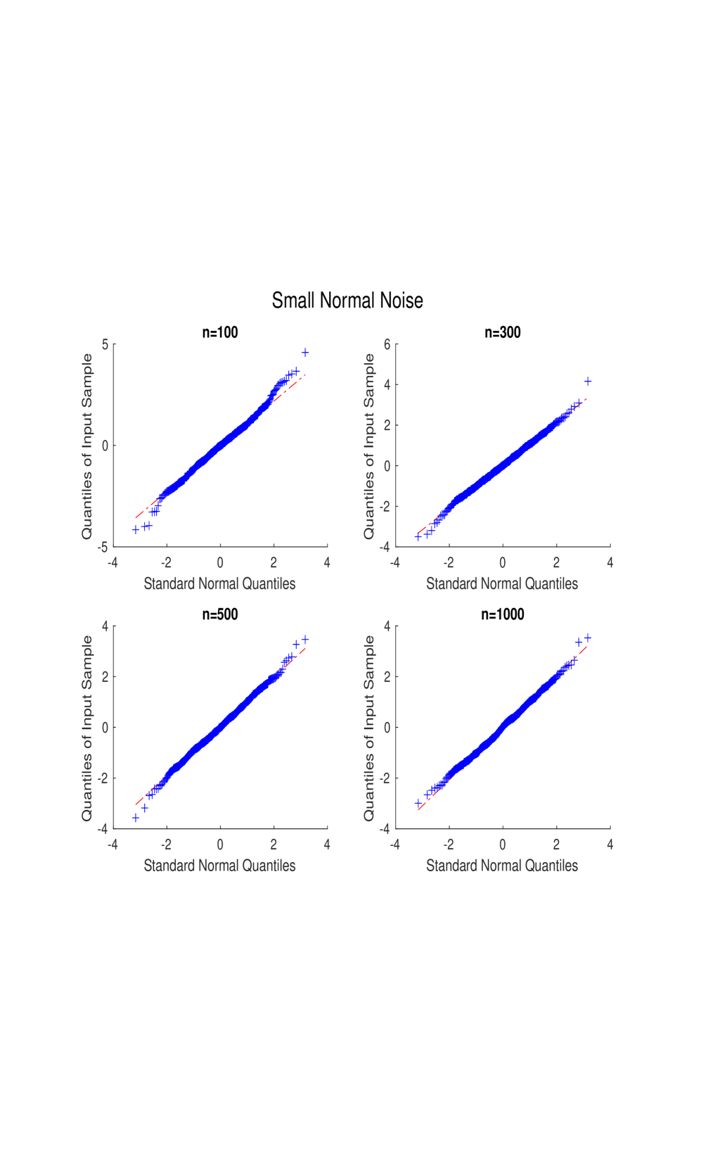
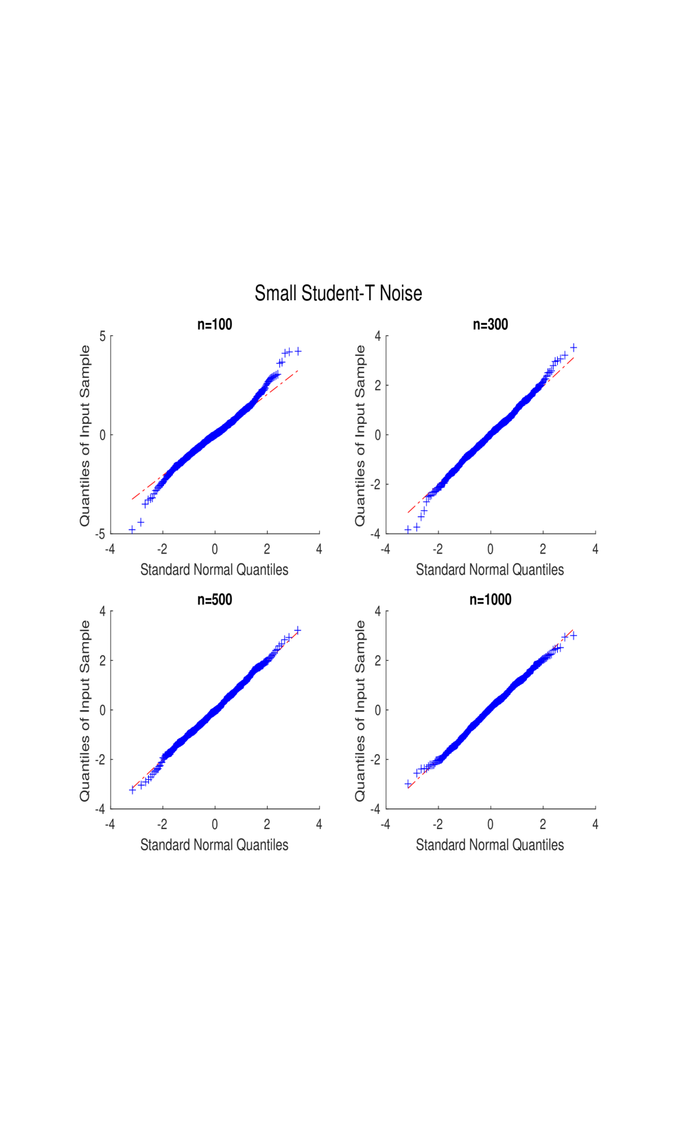
Figure 1: Results for Test Function $f_{1}$ with low-level noise $\sigma=0.5$

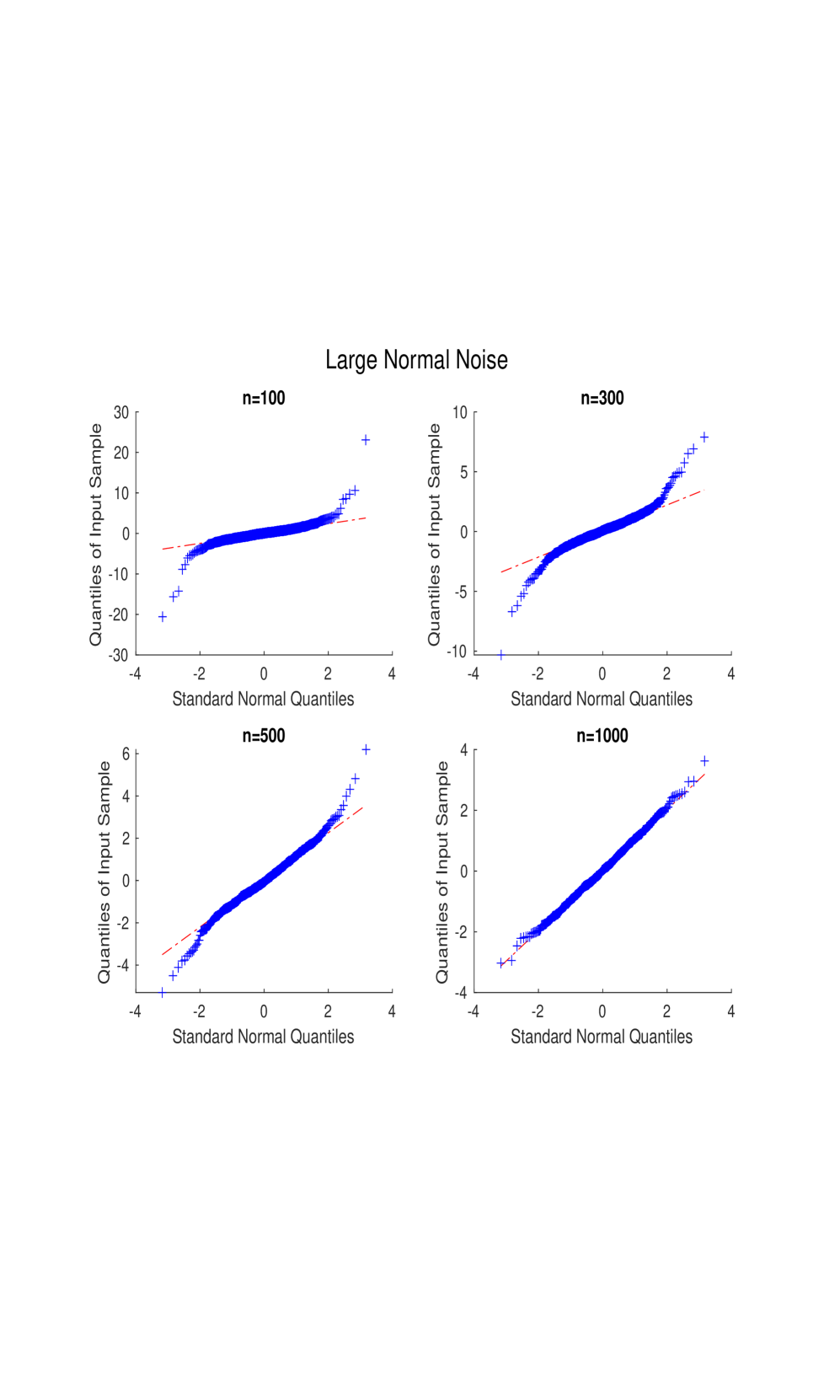
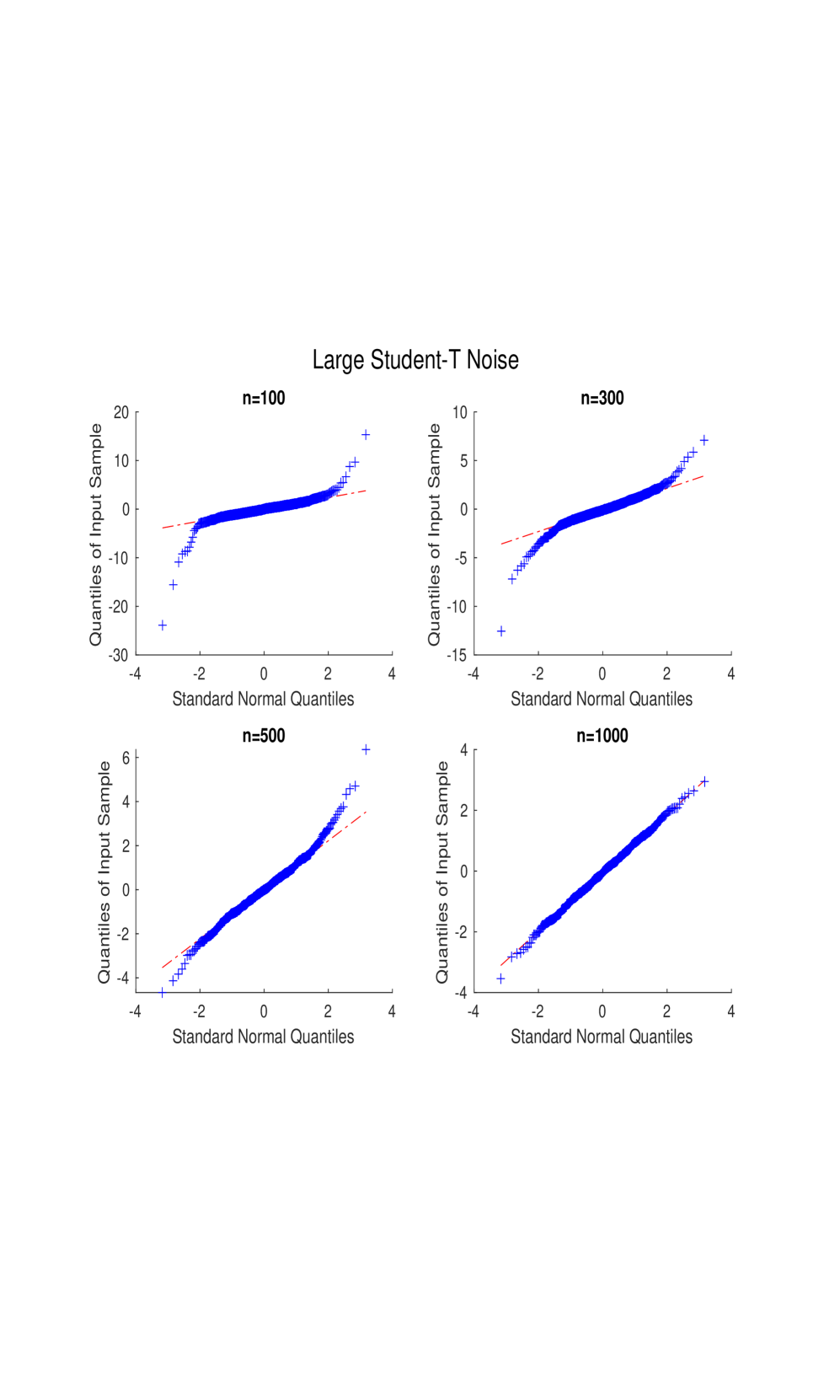
Figure 2: Results for Test Function $f_{1}$ with high-level noise $\sigma=5$

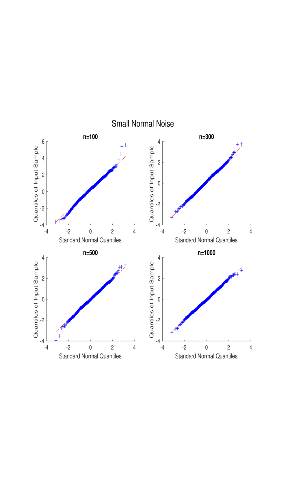
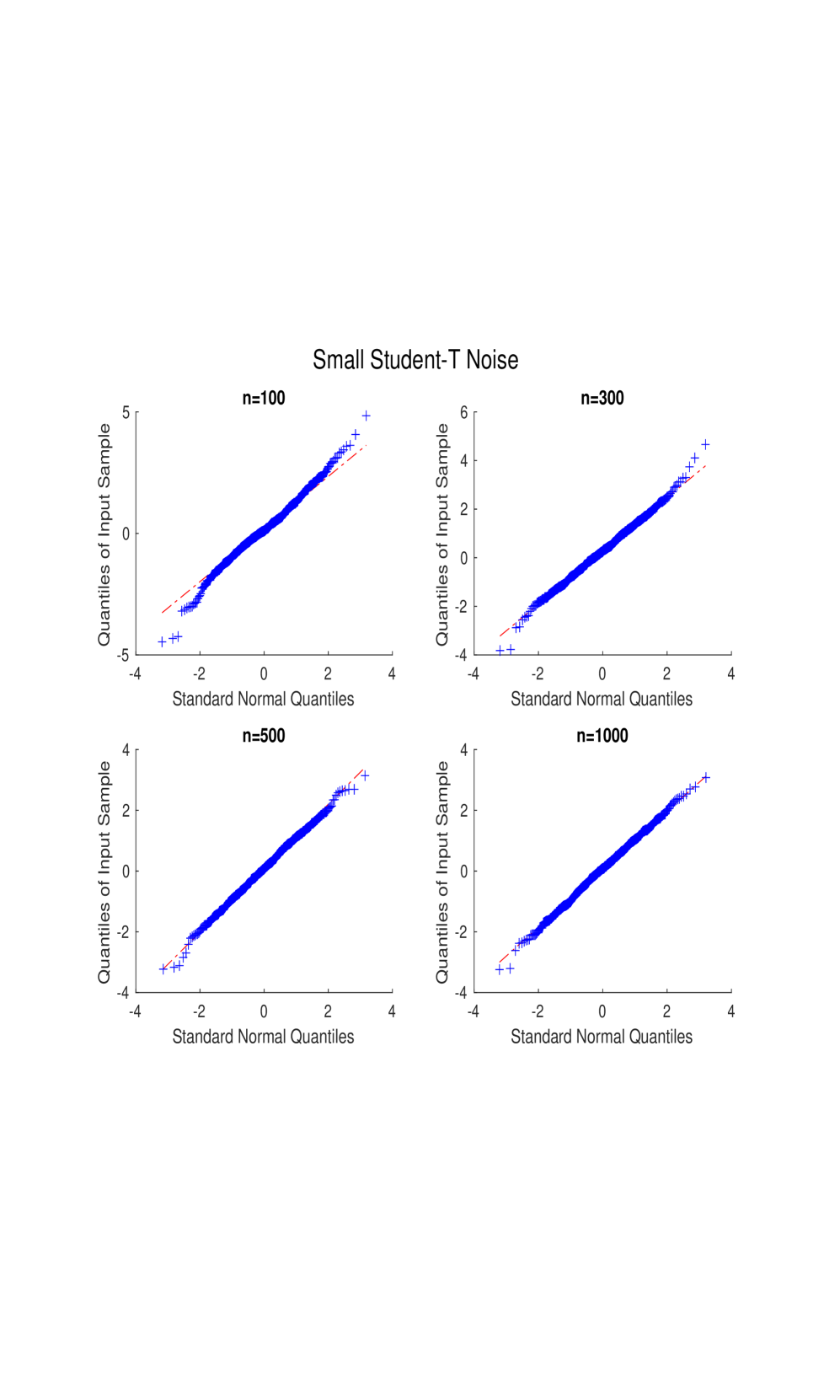
Figure 3: Results for Test Function $f_{2}$ with low-level noise $\sigma=0.5$

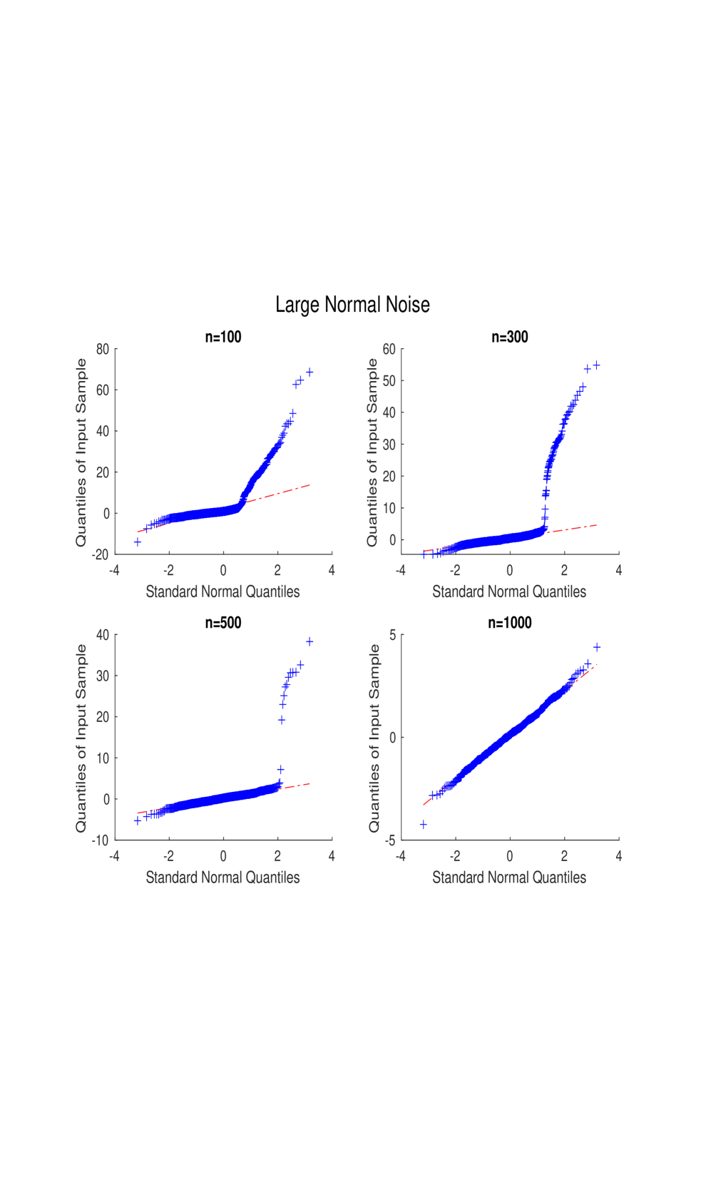
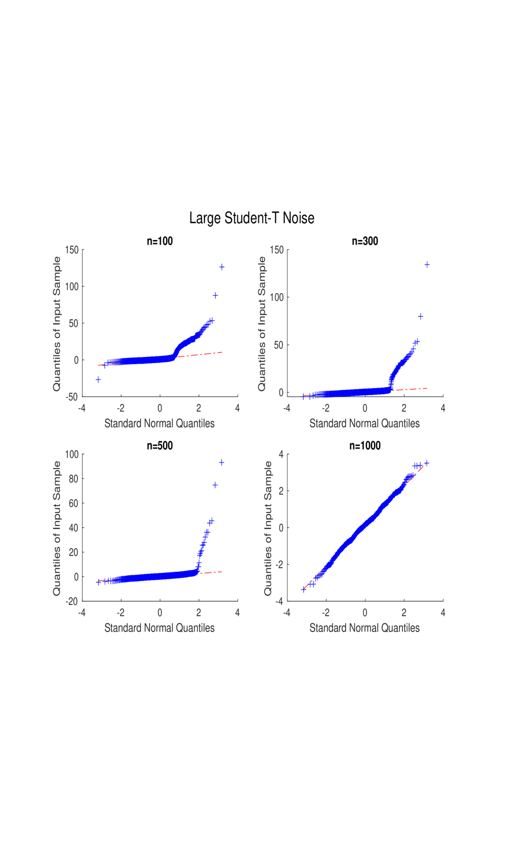
Figure 4: Results for Test Function $f_{2}$ with high-level noise $\sigma=5$

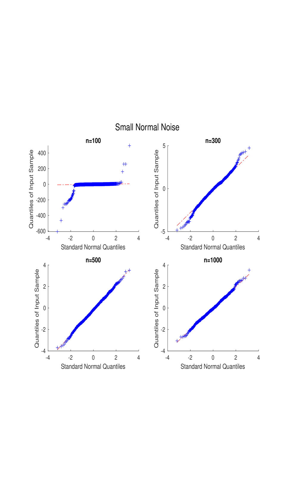
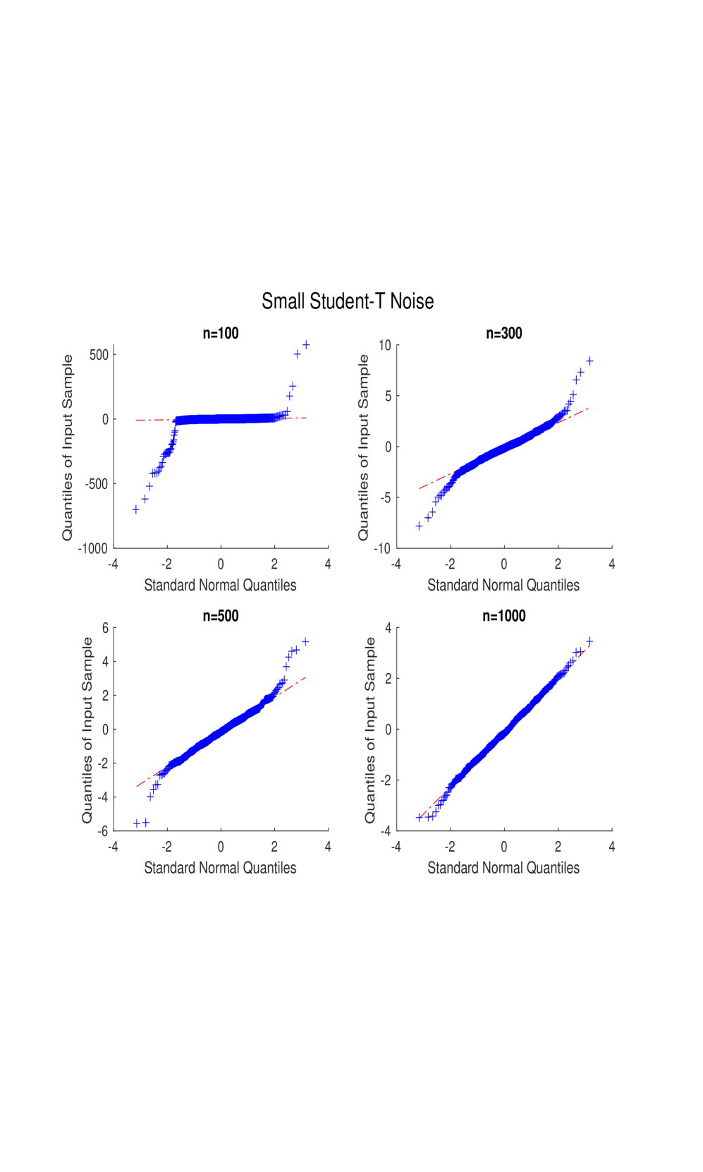
Figure 5: Results for Test Function $f_{3}$ with low-level noise $\sigma=0.5$

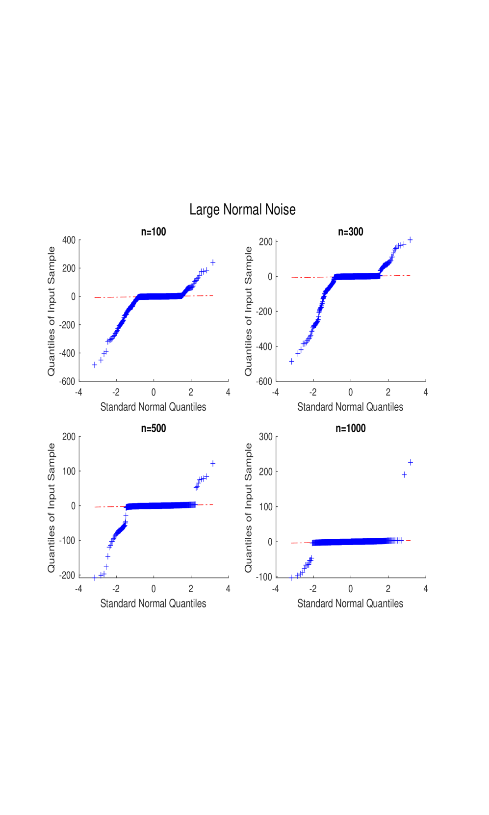
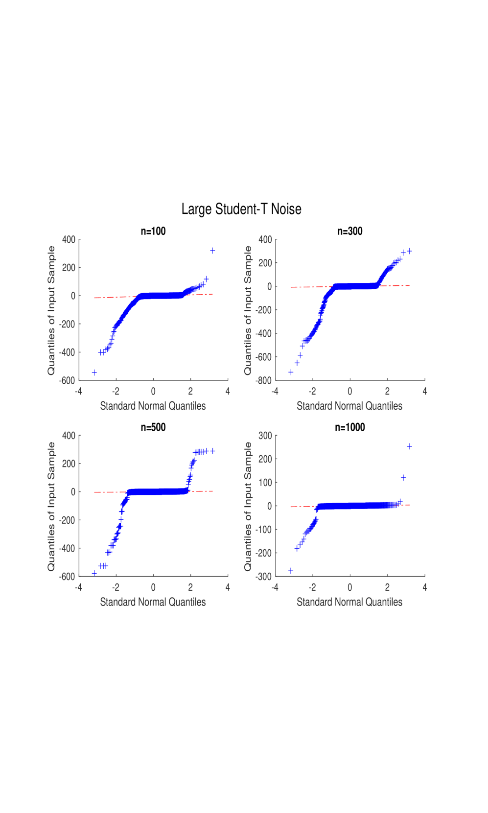
Figure 6: Results for Test Function $f_{3}$ with low-level noise $\sigma=5$

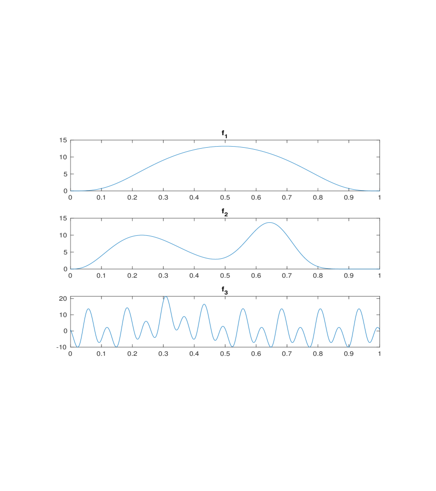
Figure 7: Plots of Three Test Functions $f_{1},f_{2},f_{3}$

Tables 2 and 3 summarize the CP of our asymptotic CI in Theorem 10 over 800 replications. Tables 2 and 3 imply that in the first two cases, the proposed asymptotic confidence intervals provide decent coverage rates (i.e., close to the nominal level $95\%$) for both functions, regardless of the type of the error distribution. For Case 3, we suffer from the under-coverage problem in high noise scenarios, KRR cannot accurately reconstruct the function and thus pinpoint the global minimum point. But such a problem is mitigated when the sample size is sufficiently large: when $n=1500$, the proposed asymptotic CI has a CP close to 0.95.

Figures 1-6 present the Q-Q plots of the aforementioned statistics over the replications. As shown in Figures 1 and 3, when the error variance is small, the distribution of statistical quantities corresponding to two different error distributions is close to the normal distribution even under small sample sizes. However, in Case 3 with small noise, the statistical values associated with the normal distribution error closely align with the normal distribution, in contrast to those associated with the $t$-distribution error. Nevertheless, as sample size increases, the statistics corresponding to both error distributions progressively approach the normal distribution. When the error variance is relatively large, as observed in Figures 2, 4, and 6, the Q-Q plots for both types of error distribution exhibit an S-shape, indicating that the statistics’ distribution has heavier tails than the normal distribution, especially with a sample of less than 500. In particular, as demonstrated in Figure 6, the statistics with both the $t$-distributed errors and normal distributed errors severally deviate from a normal distribution even under a sample size of 1000. As said before, this deviation is mainly due to the large uniform estimation errors, so we cannot correctly pinpoint which local optimal is the global optimal. Nevertheless, as exhibited in Table 2 and Table 3, the coverage rates of the test statistics associated with a normal distribution are slightly better than those with $t$-distributed errors across all sample sizes.

In view of the different simulation results led by the noise distribution, these results support our hypothesis in Remark 4 that the uniform rate of convergence of KRR depends on the tail property of the random noise.

In summary, the simulation results show that the asymptotic confidence interval for the optimal point generally aligns with our asymptotic analysis. The CP uniformly approaches the desired confidence level as the sample size grows, showing the validity of the intervals. In addition, the resulting confidence intervals are not sensitive to the error distribution.

	Coverage Probability under Normal Noise with $\alpha=0.05$
	$f_{1}$		$f_{2}$		$f_{3}$
$n$	$\sigma=0.5$	$\sigma=5$	$\sigma=0.5$	$\sigma=5$	$\sigma=0.5$	$\sigma=5$
100	0.9031	0.8010	0.8452	0.5872	0.5968	0.5978
300	0.9317	0.8304	0.9178	0.7665	0.8386	0.6223
500	0.9533	0.8821	0.9398	0.8415	0.9118	0.8344
1000	0.9543	0.9412	0.9577	0.9205	0.9441	0.8898
1500	0.9573	0.9532	0.9470	0.9389	0.9407	0.9382

Table 2: Estimated Coverage Probability for Normal Distributed Noise.

	Coverage Probability under $t_{3}$ Noise with $\alpha=0.05$
	$f_{1}$		$f_{2}$		$f_{3}$
$n$	$\sigma=0.5$	$\sigma=5$	$\sigma=0.5$	$\sigma=5$	$\sigma=0.5$	$\sigma=5$
100	0.9005	0.8101	0.8801	0.6006	0.5114	0.5578
300	0.9329	0.8412	0.9217	0.7912	0.8359	0.5976
500	0.9532	0.8897	0.9470	0.8584	0.9295	0.7716
1000	0.9402	0.9509	0.9501	0.9142	0.9310	0.8475
1500	0.9472	0.9417	0.9629	0.9401	0.9389	0.9293

Table 3: Estimated Coverage Probability for Student’s-t Distributed Noise.

6 Discussion on the Semi-parametric Effect

As shown in Proposition 2, when $\delta=1$, there exists $h$ such that $\langle g,v\rangle_{\mathcal{H}}=\langle h,v\rangle_{L_{2}}$ for each $v\in\mathcal{H}$. In this section, we will discuss the known results from the standard semi-parametric statistical theory through the lens of the proposed approach.

In the literature, it is often assumed that the input points $x_{i}$’s are independent and identically random samples. Denote the probability density function of $x_{1}$ by $p_{X}$. The semi-parametric theory gives rise to an asymptotic result

$$\sqrt{n}\int_{\Omega}(\hat{f}-f)(x)h(x)dx\xrightarrow{\mathscr{L}}N(0,\sigma^{2}\|h/p_{X}\|^{2}_{L_{2}}),$$ (40)

under $\lambda=o_{p}(n^{-1/2})$ in addition to some other conditions. Among these conditions, the most important one to our attention is

$$h/p_{X}\in\mathcal{H}.$$ (41)

The objective of this part is to further understand (40) together with the condition (41). Clearly, (40) implies that $\operatorname{BIAS}=o_{\mathbb{P}}(n^{-1/2})$, which cannot be obtained by simply applying Corollary 2 under the condition $\lambda=o(n^{-1/2})$. This implies that further improvement in the rate of convergence emerges. Also, this improvement cannot be explained using the results in Section 3.4, because here we do not make any more assumptions other than $f\in\mathcal{H}$.

To explain the actual reason, we should take a perspective of numerical integration. Define

$$\mathscr{E}:=\int_{\Omega}(\mathbb{E}_{E}\hat{f}-f)(x)h(x)dx-\frac{1}{n}\sum_{i=1}^{n}(\mathbb{E}_{E}\hat{f}-f)(x_{i})\frac{h(x_{i})}{p_{X}(x_{i})},$$ (42)

the error of approximating the integral $\int_{\Omega}(\hat{f}-f)(x)h(x)dx$ with the summation $n^{-1}\sum_{i=1}^{n}(\hat{f}-f)(x_{i})h(x_{i})/p_{X}(x_{i})$. Under our setting, $x_{i}$’s are not necessarily random, and $p_{X}$ can be any function of our choice with the goal of making $|\mathscr{E}|$ small.

We will first show that the second term in (42) is small if $h/p_{X}\in\mathcal{H}$.

Theorem 11.

If $h/p_{X}\in\mathcal{H}$,

$$\frac{1}{n}\sum_{i=1}^{n}(\mathbb{E}_{E}\hat{f}-f)(x_{i})\frac{h(x_{i})}{p_{X}(x_{i})}\leq\lambda\|f\|_{\mathcal{H}}\|h/p_{X}\|_{\mathcal{H}}.$$

Thus, regarding $\|f\|_{\mathcal{H}}$ and $\|h/p_{X}\|_{\mathcal{H}}$ as constants,

$$|\operatorname{BIAS}| = \left|\int_{\Omega}(\mathbb{E}_{E}\hat{f}-f)(x)h(x)dx\right|\leq|\mathscr{E}|+\left|\frac{1}{n}\sum_{i=1}^{n}(\mathbb{E}_{E}\hat{f}-f)(x_{i})\frac{h(x_{i})}{p_{X}(x_{i})}\right|$$

$$= |\mathscr{E}|+O(\lambda).$$

In case $x_{i}$’s are indeed independent copies with the density $p_{X}$, the standard empirical process theory [61] can show that $|\mathscr{E}|=o_{\mathbb{P}}(n^{-1/2})$, provided that $\int_{\Omega}(\mathbb{E}_{E}\hat{f}-f)^{2}(x)p_{X}(x)dx=o_{\mathbb{P}}(1)$. Hence we have recovered the results from the semi-parametric statistical literature. If the input points $X$ are carefully chosen, the integration error can be much smaller than that from a Monte Carlo sampling. For example, when $\Omega=[0,1]$ and $X$ are evenly distributed, choosing $p_{X}=1$, then $|\mathscr{E}|$ can be as small as $O(n^{-2})$. In this situation, $|\mathscr{E}|$ can be smaller than $O(\lambda)$ when $\lambda$ is not too small, which implies that the lower bound in Corollary 4 can be reached.

References

- Adams and Fournier, [2003] Adams, R. A. and Fournier, J. J. (2003). Sobolev Spaces, volume 140. Academic Press.
- Bach and Jordan, [2002] Bach, F. R. and Jordan, M. I. (2002). Kernel independent component analysis. Journal of machine learning research, 3(Jul):1–48.
- Bauer et al., [2007] Bauer, F., Pereverzev, S., and Rosasco, L. (2007). On regularization algorithms in learning theory. Journal of complexity, 23(1):52–72.
- Belloni et al., [2015] Belloni, A., Chernozhukov, V., Chetverikov, D., and Kato, K. (2015). Some new asymptotic theory for least squares series: Pointwise and uniform results. Journal of Econometrics, 186(2):345–366.
- Bordelon et al., [2020] Bordelon, B., Canatar, A., and Pehlevan, C. (2020). Spectrum dependent learning curves in kernel regression and wide neural networks. In International Conference on Machine Learning, pages 1024–1034. PMLR.
- Boser et al., [1992] Boser, B. E., Guyon, I. M., and Vapnik, V. N. (1992). A training algorithm for optimal margin classifiers. In Proceedings of the fifth annual workshop on Computational learning theory, pages 144–152.
- Brenner and Scott, [2008] Brenner, S. C. and Scott, L. R. (2008). The Mathematical Theory of Finite Element Methods, volume 3. Springer.
- Brezis and Mironescu, [2019] Brezis, H. and Mironescu, P. (2019). Where sobolev interacts with gagliardo–nirenberg. Journal of Functional Analysis, 277(8):2839–2864.
- Cai and Yuan, [2012] Cai, T. T. and Yuan, M. (2012). Minimax and adaptive prediction for functional linear regression. Journal of the American Statistical Association, 107(499):1201–1216.
- Caponnetto and De Vito, [2007] Caponnetto, A. and De Vito, E. (2007). Optimal rates for the regularized least-squares algorithm. Foundations of Computational Mathematics, 7:331–368.
- Cattaneo and Farrell, [2013] Cattaneo, M. D. and Farrell, M. H. (2013). Optimal convergence rates, bahadur representation, and asymptotic normality of partitioning estimators. Journal of Econometrics, 174(2):127–143.
- Chen, [2007] Chen, X. (2007). Large sample sieve estimation of semi-nonparametric models. Handbook of econometrics, 6:5549–5632.
- Chen and Christensen, [2015] Chen, X. and Christensen, T. M. (2015). Optimal uniform convergence rates and asymptotic normality for series estimators under weak dependence and weak conditions. Journal of Econometrics, 188(2):447–465.
- Cheng and Shang, [2013] Cheng, G. and Shang, Z. (2013). Joint asymptotics for semi-nonparametric models under penalization. arXiv preprint arXiv:1311.2628.
- Ciliberto et al., [2020] Ciliberto, C., Rosasco, L., and Rudi, A. (2020). A general framework for consistent structured prediction with implicit loss embeddings. The Journal of Machine Learning Research, 21(1):3852–3918.
- Cortes et al., [2012] Cortes, C., Mohri, M., and Rostamizadeh, A. (2012). Algorithms for learning kernels based on centered alignment. Journal of Machine Learning Research, 13(Mar):795–828.
- Cui et al., [2021] Cui, H., Loureiro, B., Krzakala, F., and Zdeborová, L. (2021). Generalization error rates in kernel regression: The crossover from the noiseless to noisy regime. Advances in Neural Information Processing Systems, 34:10131–10143.
- Demengel, [2012] Demengel, F. (2012). Functional Spaces for the Theory of Elliptic Partial Differential Equations. Springer.
- Dicker et al., [2017] Dicker, L. H., Foster, D. P., and Hsu, D. (2017). Kernel ridge vs. principal component regression: Minimax bounds and the qualification of regularization operators. Electronic Journal of Statistics, 11:1022–1047.
- Dziugaite et al., [2015] Dziugaite, G. K., Roy, D. M., and Ghahramani, Z. (2015). Training generative neural networks via maximum mean discrepancy optimization. In Proceedings of the Thirty-First Conference on Uncertainty in Artificial Intelligence, pages 258–267.
- Fischer and Steinwart, [2020] Fischer, S. and Steinwart, I. (2020). Sobolev norm learning rates for regularized least-squares algorithms. The Journal of Machine Learning Research, 21(1):8464–8501.
- Gerfo et al., [2008] Gerfo, L. L., Rosasco, L., Odone, F., Vito, E. D., and Verri, A. (2008). Spectral algorithms for supervised learning. Neural Computation, 20(7):1873–1897.
- Gretton et al., [2012] Gretton, A., Borgwardt, K. M., Rasch, M. J., Schölkopf, B., and Smola, A. (2012). A kernel two-sample test. Journal of Machine Learning Research, 13(Mar):723–773.
- Gretton et al., [2005] Gretton, A., Bousquet, O., Smola, A., and Schölkopf, B. (2005). Measuring statistical dependence with hilbert-schmidt norms. In International conference on algorithmic learning theory, pages 63–77. Springer.
- Guo et al., [2017] Guo, Z.-C., Lin, S.-B., and Zhou, D.-X. (2017). Learning theory of distributed spectral algorithms. Inverse Problems, 33(7):074009.
- Huang, [2003] Huang, J. Z. (2003). Local asymptotics for polynomial spline regression. The Annals of Statistics, 31(5):1600–1635.
- Kosorok, [2008] Kosorok, M. R. (2008). Introduction to Empirical Processes and Semiparametric Inference. Springer.
- Li et al., [2019] Li, C.-L., Chang, W.-C., Mroueh, Y., Yang, Y., and Poczos, B. (2019). Implicit kernel learning. In The 22nd International Conference on Artificial Intelligence and Statistics, pages 2007–2016. PMLR.
- Li and Zhu, [2020] Li, T. and Zhu, Z. (2020). Inference for generalized partial functional linear regression. Statistica Sinica, 30(3):1379–1397.
- Li et al., [2022] Li, Y., Zhang, H., and Lin, Q. (2022). On the saturation effect of kernel ridge regression. In The Eleventh International Conference on Learning Representations.
- Li et al., [2023] Li, Y., Zhang, H., and Lin, Q. (2023). On the asymptotic learning curves of kernel ridge regression under power-law decay. arXiv preprint arXiv:2309.13337.
- Lian et al., [2021] Lian, H., Liu, J., and Fan, Z. (2021). Distributed learning for sketched kernel regression. Neural Networks, 143:368–376.
- Lin et al., [2020] Lin, J., Rudi, A., Rosasco, L., and Cevher, V. (2020). Optimal rates for spectral algorithms with least-squares regression over hilbert spaces. Applied and Computational Harmonic Analysis, 48(3):868–890.
- Lin et al., [2017] Lin, S.-B., Guo, X., and Zhou, D.-X. (2017). Distributed learning with regularized least squares. The Journal of Machine Learning Research, 18(1):3202–3232.
- Liu et al., [2023] Liu, R., Li, K., and Li, M. (2023). Estimation and hypothesis testing of derivatives in smoothing spline anova models. arXiv preprint arXiv:2308.13905.
- Liu and Li, [2020] Liu, Z. and Li, M. (2020). On the estimation of derivatives using plug-in KRR estimators. arXiv preprint arXiv:2006.01350.
- Loureiro et al., [2021] Loureiro, B., Gerbelot, C., Cui, H., Goldt, S., Krzakala, F., Mezard, M., and Zdeborová, L. (2021). Learning curves of generic features maps for realistic datasets with a teacher-student model. Advances in Neural Information Processing Systems, 34:18137–18151.
- Lv et al., [2023] Lv, S., He, X., and Wang, J. (2023). Kernel-based estimation for partially functional linear model: Minimax rates and randomized sketches. Journal of Machine Learning Research, 24(55):1–38.
- Mammen and van de Geer, [1997] Mammen, E. and van de Geer, S. (1997). Penalized quasi-likelihood estimation in partial linear models. The Annals of Statistics, 25(3):1014–1035.
- Marteau-Ferey et al., [2019] Marteau-Ferey, U., Ostrovskii, D., Bach, F., and Rudi, A. (2019). Beyond least-squares: Fast rates for regularized empirical risk minimization through self-concordance. In Conference on learning theory, pages 2294–2340. PMLR.
- Mendelson and Neeman, [2010] Mendelson, S. and Neeman, J. (2010). Regularization in kernel learning. Ann. Statist., 38(1):526–565.
- Messer and Goldstein, [1993] Messer, K. and Goldstein, L. (1993). A new class of kernels for nonparametric curve estimation. The Annals of Statistics, pages 179–195.
- Pourkamali-Anaraki et al., [2020] Pourkamali-Anaraki, F., Hariri-Ardebili, M. A., and Morawiec, L. (2020). Kernel ridge regression using importance sampling with application to seismic response prediction. In 2020 19th IEEE International Conference on Machine Learning and Applications (ICMLA), pages 511–518. IEEE.
- Rastogi and Sampath, [2017] Rastogi, A. and Sampath, S. (2017). Optimal rates for the regularized learning algorithms under general source condition. Frontiers in Applied Mathematics and Statistics, 3:3.
- Schölkopf et al., [2001] Schölkopf, B., Herbrich, R., and Smola, A. J. (2001). A generalized representer theorem. In International Conference on Computational Learning Theory, pages 416–426. Springer.
- Shang, [2010] Shang, Z. (2010). Convergence rate and bahadur type representation of general smoothing spline m-estimates. Electronic Journal of Statistics, 4:1411–1442.
- Shang and Cheng, [2013] Shang, Z. and Cheng, G. (2013). Local and global asymptotic inference in smoothing spline models. The Annals of Statistics, 41(5):2608–2638.
- Silverman, [1984] Silverman, B. W. (1984). Spline smoothing: the equivalent variable kernel method. The annals of Statistics, pages 898–916.
- Singh et al., [2019] Singh, R., Sahani, M., and Gretton, A. (2019). Kernel instrumental variable regression. Advances in Neural Information Processing Systems, 32.
- [50] Singh, R. and Vijaykumar, S. Kernel ridge regression inference with applications to preference data.
- Singh et al., [2020] Singh, R., Xu, L., and Gretton, A. (2020). Kernel methods for causal functions: Dose, heterogeneous, and incremental response curves. arXiv preprint arXiv:2010.04855.
- Smale and Zhou, [2007] Smale, S. and Zhou, D.-X. (2007). Learning theory estimates via integral operators and their approximations. Constructive approximation, 26(2):153–172.
- Steinwart et al., [2009] Steinwart, I., Hush, D. R., Scovel, C., et al. (2009). Optimal rates for regularized least squares regression. In COLT, pages 79–93.
- Stone, [1980] Stone, C. J. (1980). Optimal rates of convergence for nonparametric estimators. The Annals of Statistics, 8(6):1348–1360.
- Stone, [1982] Stone, C. J. (1982). Optimal global rates of convergence for nonparametric regression. The Annals of Statistics, pages 1040–1053.
- Sun et al., [2018] Sun, X., Du, P., Wang, X., and Ma, P. (2018). Optimal penalized function-on-function regression under a reproducing kernel hilbert space framework. Journal of the American Statistical Association, 113(524):1601–1611.
- Talwai et al., [2022] Talwai, P., Shameli, A., and Simchi-Levi, D. (2022). Sobolev norm learning rates for conditional mean embeddings. In International conference on artificial intelligence and statistics, pages 10422–10447. PMLR.
- Tuo and Bhattacharya, [2023] Tuo, R. and Bhattacharya, R. (2023). Privacy-aware Gaussian process regression. arXiv preprint arXiv:2305.16541.
- Tuo et al., [2020] Tuo, R., Wang, Y., and Jeff Wu, C. (2020). On the improved rates of convergence for Matérn-type kernel ridge regression with application to calibration of computer models. SIAM/ASA Journal on Uncertainty Quantification, 8(4):1522–1547.
- Tuo and Wu, [2015] Tuo, R. and Wu, C. F. J. (2015). Efficient calibration for imperfect computer models. The Annals of Statistics, 43(6):2331–2352.
- van de Geer, [2000] van de Geer, S. A. (2000). Empirical Processes in M-Estimation, volume 6. Cambridge University Press.
- Wahba, [1978] Wahba, G. (1978). Improper priors, spline smoothing and the problem of guarding against model errors in regression. Journal of the Royal Statistical Society Series B: Statistical Methodology, 40(3):364–372.
- Wahba, [1990] Wahba, G. (1990). Spline Models for Observational Data, volume 59. SIAM.
- Wahba and Wold, [1975] Wahba, G. and Wold, S. (1975). Periodic splines for spectral density estimation: The use of cross validation for determining the degree of smoothing. Communications in Statistics – Theory and Methods, 4(2):125–141.
- Wang, [2021] Wang, W. (2021). On the inference of applying gaussian process modeling to a deterministic function. Electronic Journal of Statistics, 15(2):5014–5066.
- Wendland, [2004] Wendland, H. (2004). Scattered Data Approximation, volume 17. Cambridge University Press.
- Xiao, [2019] Xiao, L. (2019). Asymptotic theory of penalized splines. Electronic Journal of Statistics, 13(1).
- Xiao and Pennington, [2022] Xiao, L. and Pennington, J. (2022). Precise learning curves and higher-order scaling limits for dot product kernel regression. arXiv preprint arXiv:2205.14846.
- Yang et al., [2017] Yang, Y., Bhattacharya, A., and Pati, D. (2017). Frequentist coverage and sup-norm convergence rate in gaussian process regression. arXiv preprint arXiv:1708.04753.
- Yuan and Cai, [2010] Yuan, M. and Cai, T. T. (2010). A reproducing kernel hilbert space approach to functional linear regression.
- Zhang et al., [2023] Zhang, H., Li, Y., Lu, W., and Lin, Q. (2023). On the optimality of misspecified kernel ridge regression. arXiv preprint arXiv:2305.07241.
- Zhao et al., [2021] Zhao, S., Liu, R., and Shang, Z. (2021). Statistical inference on panel data models: A kernel ridge regression method. Journal of Business & Economic Statistics, 39(1):325–337.
- Zien and Ong, [2007] Zien, A. and Ong, C. S. (2007). Multiclass multiple kernel learning. In Proceedings of the 24th international conference on Machine learning, pages 1191–1198.