Parent Berry curvature and the ideal anomalous Hall crystal

Abstract

We study a model of electrons moving in a parent band of uniform Berry curvature. At sufficiently high parent Berry curvature, we show that strong repulsive interactions generically leads to the formation of an anomalous Hall crystal: a topological state with spontaneously broken continuous translation symmetry. Our results are established via a mapping to a problem of Wigner crystallization in a regular 2D electron gas. We further show that the resulting quasiparticle bands are “ideal” for realizing fractionalized topological states. Our theory provides a unified perspective for understanding several aspects of the recently observed integer and fractional quantum anomalous Hall effects in rhombohedral pentalayer graphene.

I Introduction

Electron interactions and topology can cooperate to create fascinating states of matter. This has been made abundantly clear in the field of 2D materials, where much exciting progress has been made in the study of topological flat band systems [1, 2]. In materials like twisted bilayer graphene (TBG) [3, 4, 5] or twisted transition metal dichalcogenides  [6, 7], a moiré superlattice leads to the formation of topological flat minibands which, when partially occupied, provides an ideal setting for interactions and topology to dominate. This has led to the recent experimental realization of exotic correlated topological states such as fractional Chern insulators  [8, 9, 10, 11, 12, 13, 14] at zero magnetic field  [15, 16, 17, 18, 19]. Very recent observations of the fractional quantum spin Hall effect  [20] is further evidence that novel states of matter, never seen before, are now becoming reality in topological flat band systems.

There is another setting, without flat bands (at the single-particle level), in which electronic topology and interactions can be at the forefront. Consider a system of electrons at a semiconductor band edge, which we will refer to as the “parent” band. Here, the density of electrons is low enough that the atomic Brillouin zone is irrelevant. When the parent band is topologically trivial, the system is a usual 2D electron gas (2DEG). In the presence of strong repulsive interactions, the 2DEG can spontaneously crystallize to form a Wigner crystal state  [21]. However, as will be made clear, topology becomes unavoidable when the parent band carries a high concentration of Berry curvature near its band edge, as illustrated in Fig 1. In the presence of strong repulsive interactions, it is possible that electrons in this topological parent band may spontaneously crystallize to form an exotic “anomalous Hall crystal” (AHC), a topological version of the Wigner crystal with an integer Chern number  [22, 23, 24, 25] at zero magnetic field, arising from a synergistic interplay of electronic interaction and parent band topology (which can also be viewed as a supersolid [26, 27, 28]).

One class of materials with highly concentrated Berry curvature is rhombohedral multilayer graphene [29, 30, 31, 32, 33, 34, 35, 36, 37, 38, 39, 40]. We are motivated by the recent experimental observation of the integer and fractional quantum anomalous Hall (QAH) effects in rhombohedral pentalayer graphene (R5G) aligned with hBN [19], and theoretical works following [41, 42, 43, 44, 45] (see  [46, 47] for a summary). Unlike TBG or twisted MoTe₂, the single-particle miniband structure of R5G/hBN does not possess an isolated flat band [48, 49, 50, 51]. In fact, robust correlated topological states are only observed when the electrons are localized on the layer furthest from the BN-induced moiré, implying that a strong moiré potential might actually be deleterious. Intriguingly, Hartree-Fock (HF) finds the integer QAH state even without the moiré [42, 43, 45], implying that the state may be adiabatically connected to an AHC. This suggests that the parent band perspective, without moiré, is the natural starting point. Not only this, numerical diagonalization shows that partially filling the HF bands lead to fractional Chern insulators, suggesting that its quantum geometry [52] is sufficiently “ideal” for the realization of such states [9, 53, 54, 55, 56, 57, 58, 59, 60]. However, the complexity of the microscopic model and subtleties in the treatment of electronic interactions [45] pose a serious obstacle to developing a general theoretical understanding of the origin of this state. Like the chiral limit  [61] or the heavy fermion picture  [62] of TBG, there is a need for simple, controlled, and analytically tractable models that can capture the essence of this system and reveal the universal physics beneath.

Our theory fulfills this role. We explain all these puzzling observations as natural consequences of strong electronic interactions in the presence of high parent Berry curvature.

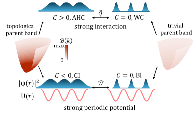
Figure 1: Summary of results and methodology. A topological parent band with a high concentration of Berry curvature $\mathcal{B}>0$ is driven into a $C>0$ anomalous Hall crystal (AHC) by strong interactions, or a $C<0$ Chern insulator (CI) by a periodic potential. These results are obtained by utilizing a unitary mapping to a model with a trivial parent band. The trivial parent band is driven to a Wigner crystal (WC) by interactions or a band insulator (BI) by a periodic potential. The AHC is mapped to the WC by a unitary transformation $\hat{Q}$, while the CI is mapped to the BI by a different unitary $\hat{W}$.

We first introduce and study a model of an idealized parent band with a uniform, continuously tunable, parent Berry curvature. This model allows us to isolate the effect of parent Berry curvature from all other extraneous details. In this model, a strong repulsive interactions and/or periodic scalar potential leads to gapped states with interesting properties and enough structure that exact statements can be made about their topology in certain limits.

We show that in the presence of a high parent Berry curvature $\mathcal{B}$, both strong interactions or a periodic potential generically drive the system into a topological state with non-zero Chern number. Consider a system of spinless electrons with uniform parent Berry curvature $\mathcal{B}\approx 2\pi N/\Omega_{\mathrm{BZ}}$, where $N$ is a positive integer and $\Omega_{\mathrm{BZ}}=4\pi^{2}n$ is the area of a Brillouin zone (chosen such that the electron density $n$ corresponds to unit filling). We demonstrate that repulsive interactions will drive the system into an AHC with Chern number $C=N$, while a commensurate periodic potential will instead lead to a Chern insulator with $C=-N$. Thus, there is very different behavior depending on whether the gap is interaction or potential-induced! Our results reveal that the two effects, repulsive interactions and a periodic potential, generically compete and drive the system to two fixed points with different topology.

These statements are established by utilizing a unitary mapping of the second-quantized Hamiltonian of a topological parent band model with $\mathcal{B}=2\pi N/\Omega_{\mathrm{BZ}}$ to a representative model with a trivial parent band $\mathcal{B}=0$. The general methodology is illustrated in Fig 1. The mapping makes use of the $2\pi$ flux periodicity of an effective momentum space Hofstadter model. Since the $\mathcal{B}=0$ state forms a trivial Wigner crystal state in the strongly interacting limit, or a trivial band insulator in a periodic potential, the properties of the $\mathcal{B}=2\pi N/\Omega_{\mathrm{BZ}}$ can be deduced. The mapping transforms the Chern number in a simple way, giving rise to the $C=\pm N$ states.

Surprisingly, our results imply a direct relation between a Wigner crystal, which is adiabatically connected to a classical state of point-like electrons, and the AHC, which is a quantum strongly interacting topological state. We exploit this mapping to write down an explicit wavefunction ansatz for the AHC state that is accurate in the limit of strong repulsive interactions. Using our wavefunction, we demonstrate that the quantum geometry of the quasiparticle bands of the AHC becomes perfectly ideal in this limit.

Finally, although we study an idealized model, we expect that our results should hold quite generally. If the parent band feature a concentrated Berry curvature near the band edge, our analysis will apply as long as the relevant low-energy states involved are within the region of high Berry curvature. We expect that our model, and the methodology developed in this work, will be useful for future studies into the role of Berry curvature in many-body physics.

II Model

II.1 General Hamiltonian

We consider general Hamiltonian describing electrons projected to a single parent band, potentially in the presence of a periodic electrostatic potential $U(\bm{r})$ and density-density interactions $V(\bm{r})$,

$$\hat{\mathcal{H}}=\hat{\mathcal{H}_{0}}+\hat{\mathcal{H}}_{\mathrm{pot}}+\hat{\mathcal{H}}_{\mathrm{int}}$$ (1)

In second quantized notation, the kinetic term is

$$\hat{\mathcal{H}_{0}}=\sum_{\bm{k}}{c}_{\bm{k}}^{\dagger}\mathcal{E}(\bm{k}){c}_{\bm{k}}$$ (2)

where $c_{\bm{k}}^{\dagger}$ creates an electron at momentum $\bm{k}$ in the parent band, and $\mathcal{E}(\bm{k})$ is the parent band dispersion. The effect of a periodic potential $U(\bm{r})=\sum_{\bm{g}}U_{\bm{g}}e^{i\bm{g}\cdot\bm{r}}$ gives rise to the term

$$\hat{\mathcal{H}}_{\mathrm{pot}}=\sum_{\bm{k},\bm{k}^{\prime}}{c}_{\bm{k}^{\prime}}^{\dagger}U_{\bm{k}^{\prime}-\bm{k}}\mathcal{F}(\bm{k}^{\prime},\bm{k}){c}_{\bm{k}}$$ (3)

where $\mathcal{F}(\bm{k^{\prime}},\bm{k})=\innerproduct{u_{\bm{k}^{\prime}}}{u_{\bm{k}}}$ is the form factor, and $\ket{u_{\bm{k}}}$ are the periodic parts of the parent band Bloch wavefunctions. We consider a density-density interaction

$$\hat{\mathcal{H}}_{\mathrm{int}}=\frac{1}{2A}\sum_{\bm{k}_{1}\bm{k}_{2}\bm{k}_{3}\bm{k}_{4}}\tilde{V}_{\bm{k}_{1}\bm{k}_{2}\bm{k}_{3}\bm{k}_{4}}{c}_{\bm{k}_{1}}^{\dagger}{c}_{\bm{k}_{2}}^{\dagger}{c}_{\bm{k}_{3}}c_{\bm{k}_{4}}$$ (4)

where $A$ is the total area of the system, and

$$\begin{split}\tilde{V}_{\bm{k}_{1}\bm{k}_{2}\bm{k}_{3}\bm{k}_{4}}=&V(\bm{k}_{1}-\bm{k}_{4})\mathcal{F}(\bm{k}_{1},\bm{k}_{4})\mathcal{F}(\bm{k}_{2},\bm{k}_{3})\\ &\times\delta_{\bm{k}_{1}+\bm{k}_{2}-\bm{k}_{3}-\bm{k}_{4}}\end{split}$$ (5)

where $V(\bm{q})=\int V(\bm{r})e^{-i\bm{q}\cdot\bm{r}}d\bm{r}$ is the Fourier transform of the real-space density-density interaction. This model thus far is entirely general. The Berry curvature and quantum geometry of the parent band are encoded in the form factors $\mathcal{F}$. The remainder of this section will discuss a particular microscopic model giving rise to the parent band.

II.2 Multifold band inversion model

We are interested in a special family of form factors $\mathcal{F}$. We introduce the “multifold band inversion” model,

$$\hat{\mathcal{H}}^{\mathrm{MBI}}=\sum_{\bm{k}}{a}^{\dagger}_{\bm{k}\sigma^{\prime}}H^{\mathrm{MBI}}_{\sigma^{\prime}\sigma}(\bm{k}){a}_{\bm{k}\sigma}$$ (6)

where $a^{\dagger}_{\bm{k}\sigma}$ creates an electron at momentum $k$ with an internal degree of freedom $\sigma=-S,\dots,S$ (thus describing an effective spin-$S$ fermion, although the microscopic origin is unimportant). The Bloch Hamiltonian is

$$H^{\mathrm{MBI}}_{\sigma^{\prime}\sigma}(\bm{k})=h_{0}(\bm{k})\delta_{\sigma^{\prime}\sigma}+[\bm{h}(\bm{k})\cdot\bm{S}]_{\sigma^{\prime}\sigma}$$ (7)

where

$$\bm{h}(\bm{k})=\left(vk_{x},vk_{y},\frac{|\bm{k}|^{2}}{m}+\delta\right)$$ (8)

and $h_{0}(\bm{k})=(\frac{1}{2}-S)|\bm{h}(\bm{k})|$. Here, $\bm{S}=(S^{x},S^{y},S^{z})$ are the standard spin-$S$ matrices satisfying $[S^{x},S^{y}]=iS^{z}$ and cyclic permutations thereof, and $\bm{S}^{2}=S(S+1)$. For $S=\frac{1}{2}$, $H^{\mathrm{MBI}}(\bm{k})$ is the two-band low-energy model for a topological band inversion  [63].

At each momentum $\bm{k}$, $H^{\mathrm{MBI}}(\bm{k})$ simply acts as a spin Zeeman field $\bm{h}(\bm{k})$, thus the eigenvalues are given by

$$E^{\mathrm{MBI}}_{n}(\bm{k})=h_{0}(\bm{k})+(S-n)|\bm{h}(\bm{k})|=\left(\frac{1}{2}-n\right)|\bm{h}(\bm{k})|.$$ (9)

where $n=0,\dots,2S$ is the band index. We shall focus on the highest energy band as our parent band, $E^{\mathrm{MBI}}_{0}(\bm{k})$. The purpose of the $h_{0}(\bm{k})$ term is to ensure that all other bands have negative energy, and can be assumed to be fully filled and inert. The $n=0$ band is topologically trivial for $\delta>0$, and becomes topological for $\delta<0$ with a Chern number of $C=2S$. The point $\delta=0$ describes a multifold fermion critical point in which all $2S$ bands touch at $\bm{k}=0$.

II.3 Ideal point and large $S$ limit

We now consider a special “ideal” point by setting $\delta=\delta^{*}\equiv-{mv^{2}/4}$. At this point, $H^{\mathrm{MBI}}$ has several desirable properties. The energy of the highest band becomes parabolic, $E_{0}(\bm{k})=\frac{k^{2}}{2m}+\frac{mv^{2}}{8}$. The corresponding eigenvector of $H^{\mathrm{MBI}}(\bm{k})$ in the eigenbasis of $S^{z}$ is

$$v_{\sigma}(\bm{k})=\sqrt{\frac{(2S)!}{(S-\sigma)!(S+\sigma)!}}\frac{(k_{x}-ik_{y})^{S+\sigma}M^{S-\sigma}}{(|\bm{k}|^{2}+M^{2})^{S}}$$ (10)

where $M=mv/2$. The eigenstates $\ket{u_{\bm{k}}}=\sum_{\sigma=-S}^{S}v_{\sigma}(\bm{k})\ket{\sigma}$ give rise to the form factors

$$\mathcal{F}(\bm{k}^{\prime},\bm{k})=\frac{(M^{2}+\bm{k}^{\prime}\cdot\bm{k}-i\bm{k^{\prime}}\crossproduct\bm{k})^{2S}}{(M^{2}+|\bm{k}^{\prime}|^{2})^{S}(M^{2}+|\bm{k}|^{2})^{S}}$$ (11)

where $\bm{k}\crossproduct\bm{q}\equiv k_{x}q_{y}-k_{y}q_{x}$, and the Berry curvature distribution

$$\mathcal{B}(\bm{k})=-\imaginary\sum_{\mu,\nu}[\epsilon_{\mu\nu}\innerproduct{\partial_{k_{\mu}}u_{\bm{k}}}{\partial_{k_{\nu}}u_{\bm{k}}}]=\frac{4SM^{2}}{(|\bm{k}|^{2}+M^{2})^{2}}$$ (12)

which integrates to a total Chern number of $C=\frac{1}{2\pi}\int\mathcal{B}(\bm{k})d\bm{k}=2S$ as advertised, where $\mu,\nu\in\{x,y\}$ and $\epsilon_{xy}=-\epsilon_{yx}=1$. Furthermore, the Fubini-Study metric

$$\begin{split}g^{\mathrm{FS}}_{\mu\nu}(\bm{k})&=\real\left[\innerproduct{\partial_{k_{\mu}}u_{\bm{k}}}{\partial_{k_{\nu}}u_{\bm{k}}}-\innerproduct{\partial_{k_{\mu}}u_{\bm{k}}}{u_{\bm{k}}}\innerproduct{u_{\bm{k}}}{\partial_{k_{\nu}}u_{\bm{k}}}\right]\\ &=\frac{2SM^{2}}{(|\bm{k}|^{2}+M^{2})^{2}}\delta_{\mu\nu}=\frac{1}{2}\mathcal{B}(\bm{k})\delta_{\mu\nu}\end{split}$$ (13)

exactly saturates both fundamental bounds: the trace $\Tr[g^{\mathrm{FS}}_{\mu\nu}(\bm{k})]\geq|\mathcal{B}(\bm{k})|$ and determinant $\det[g^{\mathrm{FS}}_{\mu\nu}(\bm{k})]\geq\frac{1}{4}|\mathcal{B}(\bm{k})|^{2}$ conditions, at all $\bm{k}$. In this sense, the quantum metric is the “minimal” given the Berry curvature distribution $\mathcal{B}(\bm{k})$. This model therefore allows for the systematic study of the effect of parent band Berry curvature, with minimal contributions from other quantum geometric effects. The total magnitude of $\mathcal{B}(\bm{k})$ can be tuned by $S$, and the distribution can be tuned by $M$.

The utility of this model is that it allows for an arbitrarily high total Berry curvature, which can be made arbitrarily uniform or concentrated. This should be contrasted with, say, a massive Dirac fermion in which the total Berry flux is limited to $\pi$. More generally, in the effective low-energy two-band model of rhombohedral $N$-layer graphene in a displacement field [64], $H(k)=\Delta\sigma^{z}+t(\hbar v/t)^{N}\left[(k_{x}-ik_{y})^{N}\sigma^{+}+h.c.\right]$, the total Berry flux is $N\pi$. While the total Berry flux can be made arbitrarily high, the distribution becomes highly non-uniform (it takes a ring-like shape) and the quantum metric is not minimal. Hence, $H^{\mathrm{MBI}}$ at the ideal point provides a controlled model for studying the effect of Berry curvature while minimizing other details.

In this work, we consider the case of a uniform positive Berry curvature distribution $\mathcal{B}(\bm{k})=\mathcal{B}>0$. This can be achieved by setting $M=\sqrt{4S/\mathcal{B}}$ and then taking the limit $S\rightarrow\infty$ (keeping $m$ fixed). In this limit, the form factors are given by

$$\mathcal{F}_{\mathcal{B}}(\bm{k}^{\prime},\bm{k})=\exp{-\frac{\mathcal{B}}{4}(|\bm{k}^{\prime}-\bm{k}|^{2}+2i\bm{k}^{\prime}\crossproduct\bm{k})}$$ (14)

which consists of a geometric factor $e^{-\frac{\mathcal{B}}{4}|\bm{k}^{\prime}-\bm{k}|^{2}}$ arising due to the “quantum distance” between the two states, and a phase factor which can be interpreted as a momentum space Aharonov-Bohm factor $\arg\mathcal{F}_{\mathcal{B}}(\bm{k}^{\prime},\bm{k})=\int_{\bm{k}}^{\bm{k}^{\prime}}\bm{A}(\bm{q})\cdot d\bm{q}$ with the Berry connection $\bm{A}(\bm{k})=\frac{\mathcal{B}}{2}(-k_{y},k_{x})$ playing the role of the vector potential in the symmetric gauge. We remark that Eq 14 is identical to that obtained for the lowest Landau level with magnetic length $\ell_{B}^{2}=\mathcal{B}$, but describes an unbounded spectrum of parabolically dispersing electrons.

We will utilize this limit as the parent band in the Hamiltonian Eq 1. The single-particle dispersion in $\mathcal{H}_{0}$ is given by $\mathcal{E}(\bm{k})=\frac{|\bm{k}|^{2}}{2m}$ (a constant offset has been neglected), and the form factors in $\hat{\mathcal{H}}_{\mathrm{pot,int}}$ are given by Eq 14. We define the operators $c_{\bm{k}}^{\dagger[\mathcal{B}]}$ to create a fermion in the microscopic state $e^{i\bm{k}\cdot\bm{r}}\ket{u_{\bm{k}}^{\mathcal{B}}}$ in the ideal parent band, which satisfy $\innerproduct{u_{\bm{k}^{\prime}}^{\mathcal{B}}}{u_{\bm{k}}^{\mathcal{B}}}=\mathcal{F}_{\mathcal{B}}(\bm{k}^{\prime},\bm{k})$. We will typically neglect the $\mathcal{B}$ superscript on $c^{\dagger}_{\bm{k}}$ when it is unimportant.

III Periodic potential

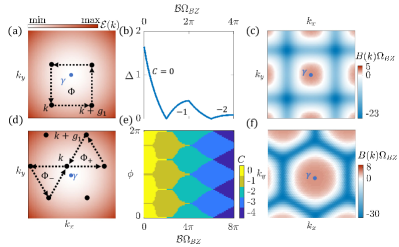
Figure 2: The ideal parent band in a periodic scalar potential. For the $C_{4}$ symmetric potential, (a) illustrates the effective momentum space square lattice Hofstadter model at each $\bm{k}$, (b) shows the gap between the first and second minibands, and the Chern number as a function of $\mathcal{B}$, and (c) shows the Berry curvature distribution. For the $C_{3}$ symmetric potential, (d) shows the effective triangular lattice Hofstadter model, (e) shows the Chern number as a function of $\mathcal{B}$ and potential shape parameter $\phi$, and (f) shows the Berry curvature. Parameters used for (b,e) are $m=\frac{1}{2}$, $g=1$, and $U_{0}=1$ ($U_{0}=5$) and (c,f) $\mathcal{B}\Omega_{\mathrm{BZ}}=2\pi$, $U_{0}=1$ ($U_{0}=0.5$,$\phi=\pi$), for the $C_{4}$ ($C_{3}$) symmetric potential.

We now consider the effect of the periodic potential $\hat{\mathcal{H}}_{\mathrm{pot}}$. Let us focus first on the $C_{4}$ symmetric potential with period $a$,

$$\begin{split}U(\bm{r})=&-2U_{0}\left(\cos(\frac{2\pi x}{a})+\cos(\frac{2\pi y}{a})\right)\\ =&-U_{0}\sum_{j=1}^{4}e^{i\bm{b}_{j}\cdot\bm{r}}\end{split}$$ (15)

where $\bm{b}_{j}=g(\cos(\frac{\pi(j-1)}{2}),\sin(\frac{\pi(j-1)}{2}))$ are reciprocal lattice vectors, and $g=\frac{2\pi}{a}$.

The Hamiltonian takes the form $\hat{\mathcal{H}}=\hat{\mathcal{H}}_{0}+\hat{\mathcal{H}}_{\mathrm{pot}}$, with

$$\begin{split}\hat{\mathcal{H}}_{0}=&\sum_{\bm{k},\bm{g}}\mathcal{E}(\bm{k}+\bm{g})c^{\dagger}_{\bm{k},\bm{g}}c_{\bm{k},\bm{g}}\\ \hat{\mathcal{H}}_{\mathrm{pot}}=&-U_{0}e^{-\frac{\mathcal{B}}{4}g^{2}}\sum_{\bm{k},\bm{g},j}c^{\dagger}_{\bm{k},\bm{g}+\bm{b}_{j}}e^{i\frac{\mathcal{B}}{2}(\bm{k}+\bm{g})\crossproduct\bm{b}_{j}}c_{\bm{k},\bm{g}}\end{split}$$ (16)

where $c_{\bm{k},\bm{g}}=c_{\bm{k}+\bm{g}}$ and, from this point onwards, $\bm{k}$ are momenta within the first Brillouin zone (which remains a good quantum number), and $\bm{g}$ are reciprocal lattice vectors. The periodic potential causes the original dispersion $\mathcal{E}(\bm{k})$ to split into multiple minibands. The prospect of engineering topological minibands from parent bands with non-trivial topology has been recently explored [65, 66, 67, 68, 69, 70]. In general, the miniband structure and topology depend crucially on the quantum geometry of the original band .

For each $\bm{k}$, $\hat{\mathcal{H}}=\hat{\mathcal{H}}_{0}+\hat{\mathcal{H}}_{\mathrm{pot}}$ can be mapped exactly to a momentum space version of the Hofstadter tight binding model  [72] on the square lattice of sites $\bm{g}_{n_{1}n_{2}}=n_{1}\bm{b}_{1}+n_{2}\bm{b}_{2}$, ($n_{1},n_{2}\in\mathbb{Z}$), with hopping amplitude $-U_{0}e^{-\frac{\mathcal{B}}{4}g^{2}}$, in the presence of a uniform a magnetic field $\mathcal{B}$ and a parabolic confining potential $\mathcal{E}(\bm{k}+\bm{g}_{n_{1}n_{2}})$, as illustrated in Fig 2a. This Hofstadter model has an effective magnetic flux of $\Phi=\mathcal{B}\Omega_{\mathrm{BZ}}$ through each plaquette, where $\Omega_{\mathrm{BZ}}=g^{2}$. Crucially, the properties of the Hofstadter model depends only on the magnetic flux modulo $2\pi$. This implies a relation between the Hamiltonian with $\mathcal{B}$ to that with $\mathcal{B}+2\pi/\Omega_{\mathrm{BZ}}$. We now establish this periodicity, and use it to make exact statements about the the resulting minibands.

Consider the unitary transformation

$$\hat{W}c_{\bm{k},\bm{g}}^{\dagger[\mathcal{B}]}\hat{W}^{\dagger}=W_{\bm{g}}(\bm{k})c_{\bm{k},\bm{g}}^{\dagger[\mathcal{B}+2\pi/\Omega_{\mathrm{BZ}}]}$$ (17)

which shifts $\mathcal{B}$ in the creation/annihilation operators, but more importantly applies a phase factor

$$W_{\bm{g}}(\bm{k})=\exp{i\pi\left(\frac{\bm{k}\crossproduct\bm{g}}{\Omega_{\mathrm{BZ}}}+\omega(\bm{g})\right)}$$ (18)

where $\omega(\bm{g})=g_{x}g_{y}/g^{2}=n_{1}n_{2}$. This transformation leaves the kinetic term $\hat{\mathcal{H}}_{0}$ invariant (it affects the microscopic wavefunctions created by $c^{\dagger}_{\bm{k}}$, but the form of the second quantized Hamiltonian is unchanged)

The reason for the phase factors is so that $\hat{W}$ will transform $\hat{\mathcal{H}}_{\mathrm{pot}}$, when viewed as a function of $\mathcal{B}$ and $U_{0}$, according to

$$\hat{\mathcal{H}}_{\mathrm{pot}}[\mathcal{B}+2\pi/\Omega_{\mathrm{BZ}},U_{0}]=\hat{W}\hat{\mathcal{H}}_{\mathrm{pot}}[\mathcal{B},U_{0}e^{-\frac{\pi}{2}}]\hat{W}^{\dagger}$$ (19)

Thus implying that the total spectrum of $\hat{\mathcal{H}}$ is periodic under a shift of $\mathcal{B}$ by $2\pi/\Omega_{\mathrm{BZ}}$, provided we also rescale the potential strength $U_{0}$. The phase factors $W_{\bm{g}}(\bm{k})$ can be interpreted as the “gauge transformation” which adds $2\pi$ flux to the momentum space Hofstadter model, and the rescaling of $U_{0}$ corrects for the quantum distance factor in $\mathcal{F}$.

Despite the spectrum being periodic, we now demonstrate that topology is not. Specifically,

$$C[\mathcal{B}+2\pi/\Omega_{\mathrm{BZ}},U_{0}]=C[\mathcal{B},U_{0}e^{-\frac{\pi}{2}}]-1$$ (20)

where $C$ is the Chern number of (any) isolated miniband. Thus, counter-intuitively, an increase of the parent band Berry curvature by $2\pi/\Omega_{\mathrm{BZ}}$ results in a decrease of the miniband Chern number by $1$.

To prove Eq 20, we consider the first quantized wavefunction of $\hat{\mathcal{H}}[\mathcal{B}_{0},U_{0}e^{-\frac{\pi}{2}}]$ in a single isolated band, $|\psi_{\bm{k}}^{(0)}\rangle=\sum_{\bm{g}}\psi_{\bm{g}}^{(0)}(\bm{k})e^{i(\bm{k}+\bm{g})\cdot\bm{r}}|u^{\mathcal{B}_{0}}_{\bm{k}+\bm{g}}\rangle$. As a result of Eq 19, the wavefunction

$$|\psi^{(1)}_{\bm{k}}\rangle=\sum_{\bm{g}}W_{\bm{g}}(\bm{k})\psi^{(0)}_{\bm{g}}(\bm{k})e^{i(\bm{k}+\bm{g})\cdot\bm{r}}|u_{\bm{k}+\bm{g}}^{\mathcal{B}_{1}}\rangle$$ (21)

is the corresponding eigenstate of $\mathcal{H}[\mathcal{B}_{1},U_{0}]$, where $\mathcal{B}_{1}=\mathcal{B}_{0}+2\pi/\Omega_{\mathrm{BZ}}$. We use the superscripts $(0)$ to denote things relating to the $\mathcal{B}_{0}$ model, and $(1)$ to denote those relating to $\mathcal{B}_{1}$. The Berry curvature is calculated from the cell-periodic part of the wavefunction, $e^{-i\bm{k}\cdot\bm{r}}|\psi_{\bm{k}}^{(1)}\rangle$, which gives rise to

$$B^{(1)}(\bm{k})=B^{\prime}(\bm{k})+\frac{\pi}{\Omega_{\mathrm{BZ}}}\sum_{\bm{g},\mu}g_{\mu}\partial_{k_{\mu}}|\psi^{(0)}_{\bm{g}}(\bm{k})|^{2}$$ (22)

where $B^{\prime}$ is the Berry curvature computed from $\sum_{\bm{g}}\psi_{\bm{g}}^{(0)}(\bm{k})e^{i\bm{g}\cdot\bm{r}}|u_{\bm{k}+\bm{g}}^{\mathcal{B}_{1}}\rangle$. It can be shown that $\int_{\mathrm{BZ}}B^{\prime}(\bm{k})d\bm{k}=\int_{\mathrm{BZ}}B^{(0)}(\bm{k})d\bm{k}=2\pi C^{(0)}$ gives the original Chern number. The final Chern number is therefore

$$C^{(1)}=\frac{1}{2\pi}\int_{\mathrm{BZ}}B^{(1)}(\bm{k})d\bm{k}=C^{(0)}-1$$ (23)

where the $-1$ is due to second term in Eq 22, which comes from the $W_{\bm{g}}(\bm{k})$ factor in $|\psi^{(1)}\rangle$. This result follows by integrating, using $|\psi^{(0)}_{\bm{g}}(\bm{k}+\bm{g}^{\prime})|=|\psi^{(0)}_{\bm{g}+\bm{g}^{\prime}}(\bm{k})|$, and performing the $\bm{g}$ summation by parts, thus proving Eq 20.

Fig 2b shows the gap and Chern number of the first band, calculated numerically, as a function of the flux, confirming this result. Fig 2c shows the Berry curvature of the first miniband, demonstrating this counter-intuitive feature. Near the $\gamma$ point of the BZ, $B(\bm{k})$ is positive (inherited from the positive parent Berry curvature), but due to superlattice effects, a gap is opened up near the zone boundaries that give rise to negative $B(\bm{k})$, precisely overcancelling the parent Berry curvature to give a negative Chern number.

We can also consider a $C_{3}$ symmetric potential,

$$U(\bm{r})=-\sum_{j=1,3,5}U_{0}e^{i\phi}e^{i\bm{b}_{j}\cdot\bm{r}}+c.c.$$ (24)

where $\bm{b}_{j}=g(\cos(\frac{\pi(j-1)}{3}),\sin(\frac{\pi(j-1)}{3}))$ and $\phi$ is a parameter that controls the shape of the potential. There are a few minor differences from the $C_{4}$ symmetric potential. First, the Hamiltonian maps to a momentum space Hofstadter model on the triangular lattice $\bm{g}_{n_{1}n_{2}}=n_{1}\bm{b}_{1}+n_{2}\bm{b}_{2}$, instead of the square lattice, with the same confining parabolic potential (Fig 2d). The hopping amplitudes are $-U_{0}e^{-\frac{\mathcal{B}}{4}g^{2}\pm i\phi}$ which, in addition to the uniform $\mathcal{B}$, give rise to an effective (staggered) magnetic flux of $\Phi_{\pm}=\frac{1}{2}\mathcal{B}\Omega_{\mathrm{BZ}}\pm 3\phi$ on each plaquette, where $\Omega_{\mathrm{BZ}}=\sqrt{3}g^{2}/2$ (each triangular plaquette has an area of $\Omega_{\mathrm{BZ}}/2$). The triangular lattice Hofstadter model comes back to itself with the addition of $\pi$ flux per plaquette, but with an opposite sign of hopping amplitudes. This manifests as the periodicity relation

$$\hat{\mathcal{H}}_{\mathrm{pot}}[\mathcal{B}_{0}+2\pi/\Omega_{\mathrm{BZ}},U_{0}]=\hat{W}\hat{\mathcal{H}}_{\mathrm{pot}}[\mathcal{B}_{0},-U_{0}e^{-\frac{\pi}{\sqrt{3}}}]\hat{W}^{\dagger}$$ (25)

with $W$ given as in Eq 18, except with $\omega(\bm{g})=(n_{1}-1)(n_{2}-1)$. Provided that the spectrum is gapped so Chern number is well defined,

$$C[\mathcal{B}_{0}+2\pi/\Omega_{\mathrm{BZ}},U_{0}]=C[\mathcal{B}_{0},-U_{0}e^{-\frac{\pi}{\sqrt{3}}}]-1$$ (26)

obeys a similar periodicity relation. Fig 2(e,f) shows the phase diagrams and Berry curvature for the $C_{3}$ symmetric potential.

A consequence of these results is that, for $\mathcal{B}=2\pi N/\Omega_{BZ}$, where $N\in\mathbb{Z}$, each isolated miniband must carry Chern number $C=-N$. This follows from both Eq 20 or Eq 26 and the fact that the Chern number must be zero for $\mathcal{B}=0$ where there is no source of time-reversal symmetry breaking. This Chern number is equal in magnitude, but opposite in sign, to the integrated parent Berry curvature over the BZ. This is true even in the limit of an infinitely strong potential.

IV Strong interactions

We now consider the effect of interactions $\hat{\mathcal{H}}_{\mathrm{int}}$, in the absence of a periodic potential so continuous translation symmetry is present. In a topologically trivial parent band ($\mathcal{B}=0$), strong interactions can lead to spontaneous breaking of continuous translation symmetry in the form of a Wigner crystal. As we shall demonstrate, strong interactions will also lead to spontaneously broken continuous translation symmetry in the presence of strong parent Berry curvature, but with non-zero Chern number, thus realizing an AHC.

In general, the periodicity in $\mathcal{B}$ is no longer an exact feature of the interacting problem. This is because the interactions involve quartic terms from different momenta $\bm{k}$, effectively coupling the momentum space Hofstadter models from different $\bm{k}$. Nevertheless, we show that there still remains a remnant of this periodicity, and that it results in topological states with the same Chern number as the parent Berry curvature $\mathcal{B}$ (opposite to our conclusions for periodic potential).

We consider the Hamiltonian $\hat{\mathcal{H}}_{0}+\hat{\mathcal{H}}_{\mathrm{int}}$, where $\hat{\mathcal{H}}_{\mathrm{int}}$ is given in Eq 4. We allow for continuous translation symmetry breaking down to a discrete unit cell with reciprocal lattice vectors $\bm{g}$ with $C_{3}$ symmetry. We assume the period is determined by the density of electrons such that there is one electron per unit cell, $\Omega_{\mathrm{BZ}}=4\pi^{2}n$ where $n$ is the electron density, as expected for a Wigner crystal. We consider decomposing the interaction into two terms, the Hartree term in which $\bm{k}_{1}=\bm{k}_{4}$, $\bm{k}_{2}=\bm{k}_{3}$, and the Fock term in which $\bm{k}_{1}=\bm{k}_{3}$, $\bm{k}_{2}=\bm{k}_{4}$ (within the BZ). That is, $\hat{\mathcal{H}}_{\mathrm{int}}\approx\hat{\mathcal{H}}_{\mathrm{H}}+\hat{\mathcal{H}}_{\mathrm{F}}$,

$$\begin{split}\hat{\mathcal{H}}_{\mathrm{H}}=\frac{1}{2A}\sum_{\begin{subarray}{c}\bm{k}_{1}\bm{k}_{2}\\ \bm{g}_{1}\bm{g}_{2}\bm{g}_{3}\bm{g}_{4}\end{subarray}}\tilde{V}^{\bm{k}_{1}\bm{k}_{2}\bm{k}_{2}\bm{k}_{1}}_{\bm{g}_{1}\bm{g}_{2}\bm{g}_{3}\bm{g}_{4}}({c}_{\bm{k}_{1}\bm{g}_{1}}^{\dagger}c_{\bm{k}_{1}\bm{g}_{4}})({c}_{\bm{k}_{2}\bm{g}_{2}}^{\dagger}{c}_{\bm{k}_{2}\bm{g}_{3}})\\ \hat{\mathcal{H}}_{\mathrm{F}}=-\frac{1}{2A}\sum_{\begin{subarray}{c}\bm{k}_{1}\bm{k}_{2}\\ \bm{g}_{1}\bm{g}_{2}\bm{g}_{3}\bm{g}_{4}\end{subarray}}\tilde{V}^{\bm{k}_{1}\bm{k}_{2}\bm{k}_{1}\bm{k}_{2}}_{\bm{g}_{1}\bm{g}_{2}\bm{g}_{3}\bm{g}_{4}}({c}_{\bm{k}_{1}\bm{g}_{1}}^{\dagger}c_{\bm{k}_{1}\bm{g}_{3}})({c}_{\bm{k}_{2}\bm{g}_{2}}^{\dagger}{c}_{\bm{k}_{2}\bm{g}_{4}})\end{split}$$ (27)

where

$$\begin{split}\tilde{V}^{\bm{k}_{1}\bm{k}_{2}\bm{k}_{3}\bm{k}_{4}}_{\bm{g}_{1}\bm{g}_{2}\bm{g}_{3}\bm{g}_{4}}=&V(\bm{k}_{1}+\bm{g}_{1}-\bm{k}_{4}-\bm{g}_{4})\mathcal{F}(\bm{k}_{1}+\bm{g}_{1},\bm{k}_{4}+\bm{g}_{4})\\ &\times\mathcal{F}(\bm{k}_{2}+\bm{g}_{2},\bm{k}_{3}+\bm{g}_{3})\times\delta(\dots)\end{split}$$ (28)

and the $\delta(\dots)$ ensures total momentum conservation. Both $\hat{\mathcal{H}}_{\mathrm{H}}$ and $\hat{\mathcal{H}}_{\mathrm{F}}$ are, at this point, still fully interacting. The HF approximation follows from a mean-field treatment of the interactions, $(c^{\dagger}c)(c^{\dagger}c)\approx\langle c^{\dagger}c\rangle c^{\dagger}c+c^{\dagger}c\langle c^{\dagger}c\rangle-\langle c^{\dagger}c\rangle\langle c^{\dagger}c\rangle$, in which $\hat{\mathcal{H}}_{\mathrm{H,F}}$ give rise to the Hartree and Fock terms respectively, and then solving the set of equations self-consistently.

Let us again consider the unitary transformation $\hat{W}$ from Eq 25. Indeed, somewhat remarkably, $\hat{\mathcal{H}}_{\mathrm{H}}$, viewed as a functional of $\mathcal{B}$ and the Fourier transform of the density-density interaction $V(q)$, satisfies the exact periodicity

$$\hat{\mathcal{H}}_{\mathrm{H}}[\mathcal{B}+2\pi/\Omega_{BZ},V(q)]=\hat{W}\hat{\mathcal{H}}_{\mathrm{H}}[\mathcal{B},V(q)e^{-\frac{\pi q^{2}}{\Omega_{BZ}}}]\hat{W}^{\dagger}$$ (29)

However, the same does not apply to the $\mathcal{H}_{\mathrm{F}}$. Instead,

$$\hat{\mathcal{H}}_{\mathrm{F}}[\mathcal{B}+2\pi/\Omega_{BZ},V(q)]=\hat{Q}\hat{\mathcal{H}}_{\mathrm{F}}[\mathcal{B},V(q)e^{-\frac{\pi q^{2}}{\Omega_{\mathrm{BZ}}}}]\hat{Q}^{\dagger}$$ (30)

where $\hat{Q}$ is defined

$$\hat{Q}c_{\bm{k},\bm{g}}^{\dagger[\mathcal{B}]}\hat{Q}^{\dagger}=W_{\bm{g}}^{*}(\bm{k})c_{\bm{k},\bm{g}}^{\dagger[\mathcal{B}+2\pi/\Omega_{\mathrm{BZ}}]}$$ (31)

Thus, there is not a single unitary transformation that accomplishes the mapping for both terms simultaneously.

The presence of this exact mapping of the quartic Hamiltonians $\hat{\mathcal{H}}_{\mathrm{H}}$ and $\hat{\mathcal{H}}_{\mathrm{F}}$ individually is quite remarkable. It is especially interesting considering that, in the periodic potential case, the momentum space Hofstadter model fails to exhibit the exact $2\pi$ flux-per-plaquette periodicity when generic longer-range hoppings are included (that is, the $\hat{\mathcal{H}}_{\mathrm{pot}}$ we consider only satisfies the exact $2\pi/\Omega_{\mathrm{BZ}}$ periodicity because the potential $U(\bm{r})$ is taken to consist of first harmonic terms $\bm{b}_{j}$). Nevertheless, both $\hat{\mathcal{H}}_{\mathrm{H}}$ and $\hat{\mathcal{H}}_{\mathrm{F}}$, which in principle contains correlated hopping terms of all ranges, enjoys this exact mapping without restriction.

We now argue that the Fock term will dominate when $\mathcal{B}$ is significant. Suppose $\mathcal{B}=2\pi N/\Omega_{\mathrm{BZ}}$. By repeated applications of $\hat{Q}^{\dagger}$, $\hat{\mathcal{H}}_{\mathrm{H}}+\hat{\mathcal{H}}_{\mathrm{F}}$ can be related to a zero-$\mathcal{B}$ Hamiltonian

$$\begin{split}\hat{Q}^{\dagger N}(\hat{\mathcal{H}}_{\mathrm{H}}&[\mathcal{B},V(q)]+\hat{\mathcal{H}}_{\mathrm{F}}[\mathcal{B},V(q)])\hat{Q}^{N}=\\ &\hat{Q}^{\dagger N}\hat{\mathcal{H}}_{\mathrm{H}}[0,\tilde{V}(q)]\hat{Q}^{N}+\hat{\mathcal{H}}_{\mathrm{F}}[0,\tilde{V}(q)]\end{split}$$ (32)

where $\tilde{V}(q)=V(q)e^{-\frac{\pi N}{\Omega_{\mathrm{BZ}}}q^{2}}$ is an effective interaction that is suppressed at large $q$ by a Gaussian factor. This corresponds to a real space interaction $\tilde{V}(r)\sim e^{-\frac{\Omega_{\mathrm{BZ}}r^{2}}{8\pi N}}I_{0}(\frac{\Omega_{\mathrm{BZ}}r^{2}}{8\pi N})$ that is smoothed off at short distances. This Hamiltonian differs from a true trivial parent band model only in the presence of various phase factors in $\hat{\mathcal{H}}_{\mathrm{H}}$ introduced by the $\hat{Q}$. However, since $\hat{\mathcal{H}}_{\mathrm{H}}$ only involves momentum transfer $q$ with a minimum of $q=g$ (the $\tilde{V}(q=0)$ term is just the total charging energy), its magnitude is more strongly suppressed by the Gaussian factor than $\hat{\mathcal{H}}_{\mathrm{F}}$, which also involves $\tilde{V}(q)$ with $0<q<g$. As a result, $\hat{\mathcal{H}}_{\mathrm{H}}$ can be neglected for large enough $\mathcal{B}$. Neglecting $\hat{\mathcal{H}}_{\mathrm{H}}$, the mapping in Eq 30 applies to the fully interacting Hamiltonian $\hat{\mathcal{H}}_{0}+\mathcal{H}_{\mathrm{F}}$ exactly.

Now, suppose we have a self-consistent solution to the HF mean field Hamiltonian at $\mathcal{B}=2\pi N/\Omega_{\mathrm{BZ}}$, with sufficiently strong interactions to create a charge gap, where the first quasiparticle band is filled. In the Fock dominated regime, the Hamiltonian is unitarily related to a zero-$\mathcal{B}$ problem with an effective interaction $\tilde{V}(q)$. The corresponding zero-$\mathcal{B}$ state describes a Wigner crystal with a filled quasiparticle band of trivial topology. By the same argument for the change in topology in Eq 20, except with the phase factors ${W}_{\bm{g}}^{*}(\bm{k})$, we conclude that the filled band of the $\mathcal{B}=2\pi N/\Omega_{\mathrm{BZ}}$ model must have a Chern number of $C=+N$, i.e. it describes an AHC.

Note that the Chern number is positive, which contrasts to the negative Chern band in the presence of a strong periodic potential. This indicates that the two limits, strong potential versus strong interactions, are distinct and, when both present, will generically compete with one another. This result is unexpected, as the two effects are typically complementary in a topologically trivial band.

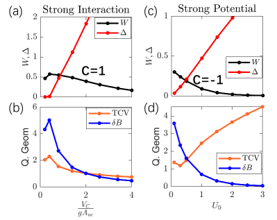
Figure 3: Energetic and quantum geometric properties of the model. (a) The charge gap $\Delta$ and bandwidth $W$ of the filled band obtained from solving the mean-field HF Hamiltonian self-consistently, as a function of Coulomb interaction strength $V_{C}$. (b) The Berry curvature fluctuation ($\delta B$) and trace condition violation (TCV) of the filled band are shown. (c,d) show corresponding quantities for a non-interacting model with a periodic potential $U_{0}$ instead. All energies are measured in units of $\frac{g^{2}}{2m}$.

To verify our analysis, we numerically solve the full self-consistent HF equations in Fig 3. We take the Coulomb interaction $V(q)=V_{C}/q$, with no periodic potential, and focus on $\mathcal{B}=2\pi/\Omega_{\mathrm{BZ}}$. The HF mean-field Hamiltonian is solved self-consistently at filling $\nu=1$ electron per unit cell. The calculation is performed in the $\ket{u_{\bm{k}+\bm{g}}}$ basis by keeping states up to a cutoff $|\bm{g}|<\Lambda$. Fig 3a shows the bandwidth of the filled quasiparticle band $W$, and charge gap $\Delta$, as a function of interaction strength $V_{C}$. Above a critical $V_{C}$, $\Delta$ becomes non-zero signaling a transition into a crystalline state with spontaneously broken continuous translation symmetry, while the bandwidth $W$ becomes small. Numerical integration of the Berry curvature, properly taking into account the wavefunction overlaps of the parent band, reveals a Chern number $C=1$, in agreement with the above analysis in the Fock-dominated regime.

To contrast, we show in Fig 3c the analogous results for a non-interacting Hamiltonian ($V_{C}=0$), in the $C_{3}$ symmetric potential $U(\bm{r})$ with $\phi=\pi$, at the same $\mathcal{B}=2\pi/\Omega_{\mathrm{BZ}}$. For any $U_{0}>0$, the gap $\Delta>0$ and bandwidth $W$ becomes very small with increasing $U_{0}$. Integration of the Berry curvature reveals that the first band is topological with $C=-1$, as expected.

We now turn to the quantum geometric properties of the resulting bands. We consider two quantum geometric indicators that have been proposed to probe the suitability of a band to realizing fractionalized phases at partial filling. We consider the Berry curvature fluctuation

$$(\delta B)^{2}=\frac{\Omega_{\mathrm{BZ}}}{4\pi^{2}}\int_{\mathrm{BZ}}(B(\bm{k})-\bar{B})^{2}d\bm{k}$$ (33)

where $\bar{B}=\Omega_{\mathrm{BZ}}^{-1}\int_{\mathrm{BZ}}B(\bm{k})d\bm{k}$, and the average trace condition violation

$$\mathrm{TCV}=\frac{1}{2\pi}\int_{\mathrm{BZ}}\left(\Tr[g^{FS}_{\mu\nu}(\bm{k})]-|B(\bm{k})|\right)d\bm{k}$$ (34)

which measures the amount by which the trace inequality, $\Tr[g^{\mathrm{FS}}_{\mu\nu}(\bm{k})]\geq|B(\bm{k})|$, is exceeded. A band with $\mathrm{TCV}=0$ is said to be “ideal” for the realization of fractional Chern insulators  [9, 53, 54, 55, 56, 57, 58, 59, 60].

We show $\delta B$ and TCV for the self-consistent HF band of the interacting model in Fig 3b, and the corresponding plot for the case of the periodic potential without interaction in Fig 3d. The Berry curvature distribution for both cases becomes increasingly uniform with $V_{C}$ or $U_{0}$. However, they differ strikingly in terms of their TCV. While the interacting $C=1$ AHC becomes increasingly ideal with strong interactions, the non-interacting $C=-1$ CI with a periodic potential is the opposite. This striking difference will be explained in the next section, based on an analytic ansatz for the wavefunctions of these two states.

V Wavefunction ansatz

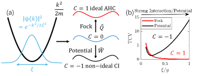
Figure 4: Wavefunction ansatz and ideal AHC. (a) Illustration of the wavefunction for the trivial $C=0$ state in the $\mathcal{B}=0$ parent band, where $\xi$ is a tuning parameter; $\xi\rightarrow\infty$ describes the limit of strong interaction or potential. By utilizing the transformation $\hat{Q}$ ($\hat{W}$), we arrive at a $C=1$ AHC ($C=-1$ CI) state for the $\mathcal{B}=2\pi/\Omega_{\mathrm{BZ}}$ model in the Fock (potential) dominated regime, respectively. (b) The trace condition violation (TCV) is shown as a function of $\xi$, demonstrating that the AHC becomes ideal as $\xi\rightarrow\infty$.

The mappings established in Sec III and IV are incredibly powerful. They manage to relate the ground states of topological quantum systems, the $C=N$ AHC or the $C=-N$ Chern insulator, to those of a topologically trivial Wigner crystal or band insulator, which can essentially be described classically. In this section, we leverage this relation to write down analytic wavefunctions based on a simple Gaussian ansatz for the trivial band insulator. Remarkably, this analytic expression fully captures and explains the emergence of the ideal HF band of the strongly interacting AHC.

First, let us consider the ground state wavefunction of the zero-$\mathcal{B}$ Hamiltonian in an infinitely strong periodic potential (with a single potential minimum per unit cell). This limit is equivalent to an array of harmonic oscillators localized at each potential minimum $\bm{R}$, each of which are described by the Gaussian wavefunction $\psi_{\bm{R}}(\bm{r})\sim\exp{-\alpha(\bm{r}-\bm{R})^{2}}$. The equivalent momentum space picture is a single isolated flat band, with the wavefunctions described by $\psi_{\bm{g}}^{(0)}(\bm{k})=\mathcal{N}_{\bm{k}}e^{-\frac{(\bm{k}+\bm{g})^{2}}{4\xi^{2}}}$ where $\xi$ is a momentum space localization length, and $\mathcal{N}_{\bm{k}}$ is a normalization constant, as illustrated in Fig 4a. Although we have considered a strong periodic potential, the ground state in the presence of an infinitely strong repulsive interaction is a classical Wigner crystal, which can also be well described by a Slater determinant of such states. We take this wavefunction as an ansatz and treat $\xi$, the momentum space localization length, as an effective parameter reflecting the overall strength of the interaction or periodic potential. This ansatz becomes exact in the strong interaction or potential limit in which $\xi\rightarrow\infty$.

Based on this, we can write down the corresponding wavefunctions for the $\mathcal{B}=2\pi/\Omega_{BZ}$ Hamiltonian. These follow from applications of either $\hat{W}$ or $\hat{Q}$. The wavefunctions are

$$|\psi_{\bm{k}}^{\pm}\rangle=\mathcal{N}_{\bm{k}}\sum_{\bm{g}}e^{-\frac{(\bm{k}+\bm{g})^{2}}{4\xi^{2}}\pm i\pi\left[\frac{\bm{k}\crossproduct\bm{g}}{\Omega_{\mathrm{BZ}}}+\omega(\bm{g})\right]}e^{i(\bm{k}+\bm{g})\cdot\bm{r}}|u_{\bm{k}+\bm{g}}^{2\pi/\Omega_{\mathrm{BZ}}}\rangle$$ (35)

where the $+$ ($-$) corresponds to the case of strong potential (interaction). The full many-body state will be a Slater determinant of $|\psi_{\bm{k}}^{\pm}\rangle$.

We directly compute the TCV of the bands described by $|\psi_{\bm{k}}^{\pm}\rangle$ in Fig 4b, as a function of $\xi$. The behavior is similar to that observed numerically from HF in Fig 3(b,d). Namely, in the strong potential limit $|\psi_{\bm{k}}^{+}\rangle$, TCV increases with increasing $\xi$, while in the strong interacting limit $|\psi_{\bm{k}}^{-}\rangle$, TCV decreases with increasing $\xi$ becoming more ideal. For large $\xi$, the trace of the Fubini-Study metric (and the Berry curvature) is $\bm{k}$-independent, and an analytic expression can be computed directly from $|\psi^{\pm}_{\bm{k}}\rangle$,

$$\Tr[g_{\mu\nu}^{\mathrm{FS}(\pm)}]=\frac{2\pi}{\Omega_{\mathrm{BZ}}}+(1\pm 1)\frac{4\pi^{2}\xi^{2}}{\Omega_{\mathrm{BZ}}^{2}}+\frac{1}{2\xi^{2}}+\mathcal{O}(e^{-\frac{2\pi^{2}\xi^{2}}{\Omega_{BZ}}})$$ (36)

thus, in the Fock-dominated AHC, the $\xi^{2}$ term is zero and $\Tr[g]-|B|\rightarrow 0$ becomes perfectly ideal at large $\xi$, in good agreement with Fig 4b. Thus, interactions separate out an ideal AHC Chern band from the parent band (reminiscent of how ideal higher Chern bands can be decomposed into ideal Chern 1 bands [73]).

VI Discussion

VI.1 Rhombohedral graphene

We first discuss our findings in the context of recent experimental and theoretical studies of rhombohedral pentalayer graphene on hBN [19, 41, 42, 43, 44, 45]. The system is described by the parent band structure of R5G, which features an electron band with a high concentration of Berry curvature at the band edge. Although the microscopic model features many detail-dependent terms, the origin of the Berry curvature can be understood from the effective low-energy two-band model describing states on the top/bottom-most layers  [64],

$$H_{\mathrm{RLG}}(\bm{k})=\begin{pmatrix}\Delta&-t(\frac{\hbar v}{t})^{L}(k_{x}-ik_{y})^{L}\\ -t(\frac{\hbar v}{t})^{L}(k_{x}+ik_{y})^{L}&-\Delta\\ \end{pmatrix}$$ (37)

where $L=5$ is the number of layers, and $\Delta$ is the effective potential difference between the top/bottom layers which can be tuned by an external displacement field, and $(v,t)\approx(0.9\times 10^{6}\mathrm{m/s},0.3\mathrm{eV})$. $H_{\mathrm{RLG}}$ describes one of a pair of spin-degenerate electron states near the $K$ valley, which also exists with their time reversed partner at the $K^{\prime}$ valley. We propose that our theory captures the essence of a single spin-valley component of the full model.

Experimentally, the integer and fractional QAH states are only observed for one sign of displacement field  [19]. Theoretical studies  [41, 42, 43, 44, 45] find that the integer and fractional QAH states appear only when the relevant parent band is localized, by the displacement field, to be on the layer located furthest from the interface with the moiré superlattice. In this regime, self-consistent HF at filling factor $\nu=1$ electron per moiré unit cell robustly find a spontaneously spin-valley-polarized state with an extremely flat and nearly ideal quasiparticle band. Exact diagonalization at fractional fillings of this HF band reveals fractional Chern insulators, in agreement with the experiment. The ideal HF band persists even in the absence of the moiré superlattice with hBN  [43, 42, 45]. It should be remarked that these theoretical studies use models for R5G that differ in various minor details, yet all arrive at the robust conclusion of the ideal HF band.

Our theory naturally explains the emergence of this ideal HF band. Namely, it is adiabatically connected to the ideal AHC in our model at $\mathcal{B}=2\pi/\Omega_{\mathrm{BZ}}$ with strong interactions. Let us first verify that the experimentally relevant Berry flux per BZ is indeed close to $2\pi$. To estimate this, we note that the Berry curvature distribution from $H_{\mathrm{RLG}}$ is concentrated at the band edge and contains a total of $5\pi$ Berry flux. This Berry flux is localized within an effective momentum space region of radius $\bar{k}\approx t/(\hbar v)$, beyond which the kinetic energy sharply increases as $E\sim(k/\bar{k})^{5}$ making those states irrelevant for the low-energy physics. This gives an effective average Berry curvature seen by the low-energy electrons of $\bar{\mathcal{B}}\approx 5/\bar{k}^{2}$. Meanwhile, the relevant density at which QAH is observed is set by the moiré superlattice at the hBN/graphene interface, with a period $a\approx 11.5$nm. Thus, using $\Omega_{\mathrm{BZ}}=8\pi^{2}/(\sqrt{3}a^{2})$, the average Berry flux per BZ is $\bar{\mathcal{B}}\Omega_{\mathrm{BZ}}\approx 1.2\times 2\pi$, which is indeed close to $2\pi$.

At $\mathcal{B}\Omega_{\mathrm{BZ}}\approx 2\pi$, our model predicts at least two competing phases, a $C=1$ ideal AHC that is favored by strong interactions, and a $C=-1$ non-ideal CI that is favored by a strong periodic potential. The HF integer QAH state in R5G is spin-valley polarized and: has same Chern sign as the parent Berry curvature , is very ideal, and appears even when the moiré superlattice is absent. These are all in agreement with our expectations based on the ideal AHC in the Fock-dominated regime of our theory. Furthermore, its absence for the opposite sign of displacement field, i.e. when the electrons are localized on the graphene layer proximate to the moiré, can be explained by the fact that the moiré essentially acts as a periodic potential, which we have shown competes with interactions. Thus, while it is likely that a weak periodic potential may help to stabilize and pin a commensurate AHC, a strong periodic potential would eventually lead to a weakening of the state and eventually a topological phase transition out of it.

VI.2 Future directions

The exact $\mathcal{B}\rightarrow\mathcal{B}+2\pi/\Omega_{\mathrm{BZ}}$ periodicity of the many-body interacting Hamiltonian $\hat{\mathcal{H}}=\hat{\mathcal{H}}_{0}+\hat{\mathcal{H}}_{\mathrm{F}}$ implies that all properties of the AHC in this model can be obtained from the corresponding properties of the corresponding WC. This includes the properties of all excited states as well. It would be interesting to analyze the resulting dynamics  [75] of the AHC through the lens of this mapping. To this end, it is therefore important to determine the effects of the interaction terms that were neglected in making the Fock-dominated $\hat{\mathcal{H}}_{\mathrm{int}}\approx\mathcal{H}_{\mathrm{F}}$ approximation. While our numerical HF analysis of the ground state with Coulomb potential is in good agreement with the physics being Fock-dominated, the neglected terms are likely to be important for other physics, such as those of excitations above the ground state.

There are many interesting direction for further study of our model, as well as possible extensions. Although we have focused in this paper on the case where either the potential or interactions dominate, there may be intermediate phases between the two that would not have an analog in the trivial parent band model. Another interesting question is the role of Berry curvature distribution: while we have focused only on the uniform case, it would be interesting to explore finite-$S$ models and the effect of the Berry curvature distribution by tuning $M$ in Eq 12. It would also be interesting to consider a “valley-ful” extension of our model, in which we allow for a time reversed partner of the parent band, which may allow for interesting valley-coherent states or excitations.

Finally, we may ask what the implications of an “ideal” AHC is, in the absence of a periodic potential. While the HF bands may be ideal for fractionalized states, the concept of fractional filling becomes somewhat dubious since the unit cell is itself defined by the electron density. However, an interesting observation is that the Berry curvature density $\mathcal{B}$ also sets a natural unit cell, $\Omega_{\mathrm{BZ}}=2\pi/\mathcal{B}$, in which there is $2\pi$ Berry flux per BZ. Fractional filling $p/q<1$ of this unit cell is equivalent to full filling of a system with a smaller Brillouin zone (enlarged unit cell) $\Omega_{\mathrm{BZ}}^{\prime}=(p/q)\Omega_{\mathrm{BZ}}$, and an effective Berry flux of $\mathcal{B}\Omega_{\mathrm{BZ}}^{\prime}=(p/q)2\pi$ per BZ. Depending on the details of the energetics, we speculate that the system may prefer fractionally filling the $\Omega_{\mathrm{BZ}}$ unit cell, rather than full filling of the $\Omega_{\mathrm{BZ}}^{\prime}$ unit cell. In this scenario, the ideal AHC band may lead to the exotic possibility of a “fractional anomalous Hall crystal” that spontaneously breaks continuous translation symmetry to form a fractional Chern insulator.

Note added — While finalizing our manuscript, a preprint appeared [76] also studying the formation of the AHC; while there is little direct overlap, our findings are all consistent.

Appendix A analytical results on the trace condition violation of ansatz wave functions

We showed numerically in the main text Fig.4 that with the gauge transformation, $\hat{Q}$ (Fock) and $\hat{W}$ (Potential), the TCV of the $C=\pm 1$ band decrease/increase as a function of $\xi$ at large $\xi$. We now give a proof for this behaviour.

Notice first that at large $\chi$ limit, the berry curvature $B(k)$ becomes uniform for both $\hat{Q}$ and $\hat{W}$ ansatz wave functions. We will not prove this statement, but satisfy ourselves to say that this is the behaviour that can be easily observed numerically. Thus the term $\int|B(\bm{k})|d\bm{k}$ in TCV is just $2\pi$ for both $\hat{Q}$ and $\hat{W}$ ansatz wave functions. We study the behaviour $\int Tr[g_{\mu\nu}^{FS}(\bm{k})]d\bm{k}$ for two ansatz wave functions at large $\xi$ limit. We will focus on the square lattice case to avoid cluttered notation, and the proof can be easily generalized to triangular lattice.

For $\hat{Q}$ ansatz (Assume that $\mathcal{B}=\frac{2\pi}{\Omega_{BZ}}=\frac{2\pi}{g^{2}}$).

$$\begin{split}&\ket{\psi^{-}(\bm{k})}\\ &=\sum_{\bm{g}}\mathcal{N}(\bm{k})e^{-\frac{(\bm{k}+\bm{g})^{2}}{4\xi^{2}}}e^{-i\frac{\pi}{g^{2}}[g_{x}g_{y}+k_{x}g_{y}-k_{y}g_{x}]}\ket{u_{\bm{k}+\bm{g}}}e^{i\bm{g}\cdot\bm{r}}\end{split}$$ (38)

If we replace the summation by an integral (we will discuss this approximation afterwards)

$$\begin{split}&\ket{\psi^{-}(\bm{k})}\\ &=\int d\bm{g}\frac{1}{\sqrt{2\pi\xi^{2}}}e^{-\frac{(\bm{k}+\bm{g})^{2}}{4\xi^{2}}}e^{-i\frac{\pi}{g^{2}}[g_{x}g_{y}+k_{x}g_{y}-k_{y}g_{x}]}\ket{u_{\bm{k}+\bm{g}}}e^{i\bm{g}\cdot\bm{r}}\end{split}$$ (39)

The $\mathcal{N}(\bm{k})\approx\frac{1}{\sqrt{2\pi\xi^{2}}}$ is obtained by requiring $\ket{\psi^{-}}$ to be normalized under this approximation. Notice that $|\innerproduct{\psi^{-}(\bm{k})}{\psi^{-}(\bm{k}+d\bm{k})}|^{2}=1-g_{\mu\nu}dk_{\mu}dk_{\nu}$. We then obtain the following

$$\begin{split}&|\innerproduct{\psi^{-}(\bm{k})}{\psi^{-}(\bm{k}+dk_{x})}|^{2}\\ &=|\int d\bm{g}\frac{1}{2\pi\xi^{2}}e^{-\frac{(\bm{k}+\bm{g})^{2}}{2\xi^{2}}}e^{\frac{{-dk_{x}^{2}}}{4\xi^{2}}}e^{-\frac{(k_{x}+g_{x})dk_{x}}{2\xi^{2}}}e^{-i\frac{\pi}{g^{2}}dk_{x}g_{y}}e^{\frac{-\pi dk_{x}^{2}}{2g^{2}}}\\ &e^{\frac{i\pi(k_{y}+g_{y})dk_{x}}{2g^{2}}}|^{2}\\ &=e^{\frac{-\pi^{2}(dk^{2}_{x})}{g^{2}}}e^{-\frac{dk^{2}_{x}}{2\xi^{2}}}|\int d\bm{g}\frac{1}{2\pi\xi^{2}}e^{-\frac{(\bm{k}+\bm{g})^{2}}{2\xi^{2}}}e^{-\frac{(k_{x}+g_{x})dk_{x}}{2\xi^{2}}}|^{2}\end{split}$$ (40)

By symmetry, it is obvious that the term inside $|..|$ is of order $1+L_{1}dk^{2}_{x}$. Thus we have an expression of $g_{xx}$ and similarly $g_{yy}$

$$\begin{split}g_{xx}=\frac{\pi}{g^{2}}+\frac{1}{2\xi^{2}}-2L_{1}\\ g_{yy}=\frac{\pi}{g^{2}}+\frac{1}{2\xi^{2}}-2L_{2}\end{split}$$ (41)

Where we have

$$L_{1}+L_{2}=\int d\bm{g}\frac{1}{2\pi\xi^{2}}e^{-\frac{(\bm{k}+\bm{g})^{2}}{2\xi^{2}}}\frac{(\bm{k}+\bm{g})^{2}}{8\xi^{4}}=\frac{1}{4\xi^{2}}$$ (42)

Thus at large $\xi$, we have

$$Tr[g_{\mu\nu}^{FS}(\hat{Q})]=\frac{2\pi}{g^{2}}+\frac{1}{2\xi^{2}}$$ (43)

We now turn to the $\hat{W}$ ansatz wave function. The analysis is exactly the same, except there will be a sign change in the gauge transformation

$$\begin{split}&|\innerproduct{\psi^{+}(\bm{k})}{\psi^{+}(\bm{k}+dk_{x})}|^{2}\\ &=|\int d\bm{g}\frac{1}{2\pi\xi^{2}}e^{-\frac{(\bm{k}+\bm{g})^{2}}{2\xi^{2}}}e^{\frac{{-dk_{x}^{2}}}{4\xi^{2}}}e^{-\frac{(k_{x}+g_{x})dk_{x}}{2\xi^{2}}}e^{i\frac{\pi}{g^{2}}dk_{x}g_{y}}e^{\frac{-\pi dk_{x}^{2}}{2g^{2}}}\\ &e^{\frac{i\pi(k_{y}+g_{y})dk_{x}}{2g^{2}}}|^{2}\\ &=e^{\frac{-\pi^{2}(dk^{2}_{x})}{g^{2}}}e^{-\frac{dk^{2}_{x}}{2\xi^{2}}}|\int d\bm{g}\frac{1}{2\pi\xi^{2}}e^{-\frac{(\bm{k}+\bm{g})^{2}}{2\xi^{2}}}e^{-\frac{(k_{x}+g_{x})dk_{x}}{2\xi^{2}}}e^{i\frac{2\pi}{g^{2}}dk_{x}g_{y}}|^{2}\end{split}$$ (44)

In that case, we will have

$$\begin{split}&|\int d\bm{g}\frac{1}{2\pi\xi^{2}}e^{-\frac{(\bm{k}+\bm{g})^{2}}{2\xi^{2}}}e^{-\frac{(k_{x}+g_{x})dk_{x}}{2\xi^{2}}}e^{i\frac{2\pi}{g^{2}}dk_{x}g_{y}}|^{2}\\ &=|\int d\bm{\eta}\frac{1}{2\pi\xi^{2}}e^{-\frac{\bm{\eta}^{2}}{2\xi^{2}}}e^{-\frac{\eta_{x}dk_{x}}{2\xi^{2}}}e^{i\frac{2\pi}{g^{2}}dk_{x}\eta_{y}}|^{2}\\ &\approx|1+\int d\bm{\eta}\frac{e^{-\frac{\bm{\eta}}{2\xi^{2}}}}{2\pi\xi^{2}}\frac{dk^{2}_{x}}{2}(\frac{2i\pi}{g^{2}}{\eta_{y}}-\frac{\eta_{x}}{2\xi^{2}})^{2}|^{2}\end{split}$$ (45)

Thus, we will have

$$\begin{split}&L_{1}+L_{2}\\ &=\int d\bm{g}\frac{1}{2\pi\xi^{2}}e^{-\frac{(\bm{k}+\bm{g})^{2}}{2\xi^{2}}}(\bm{k}+\bm{g})^{2}(\frac{1}{8\xi^{4}}-\frac{2\pi^{2}}{g^{4}})\\ &=\frac{1}{4\xi^{2}}-\frac{4\pi^{2}\xi^{2}}{g^{4}}\end{split}$$ (46)

Then at large $\xi$

$$Tr[g_{\mu\nu}^{FS}(\hat{W})]=\frac{2\pi}{g^{2}}+\frac{1}{2\xi^{2}}+\frac{8\pi^{2}\xi^{2}}{g^{4}}$$ (47)

Now, we notice that when we replaced the $\sum_{\bm{g}}$ by $\int d\bm{g}$, we are effectively ignoring the $\bm{k}$ dependence of the trace. We could have been more careful with the momentum dependence. But it turns out that those terms are not super important in understanding the physics. Let me now show this point: The properly normalized $\hat{Q}$ ansatz wavefunction $\ket{\psi^{-}(\bm{k})}$ is

$$\begin{split}&\ket{\psi^{-}(\bm{k})}\\ &=\sum_{\bm{g}}\mathcal{N}(\bm{k})e^{-\frac{(\bm{k}+\bm{g})^{2}}{4\xi^{2}}}e^{-i\frac{\pi}{g^{2}}[g_{x}g_{y}+k_{x}g_{y}-k_{y}g_{x}]}\ket{u_{\bm{k}+\bm{g}}}e^{i\bm{g}\cdot\bm{r}}\end{split}$$ (48)

Where the normalization constant is the following, with $z_{x/y}=\frac{k_{x/y}\pi}{g}$, $q=\exp(-\frac{2\pi^{2}\xi^{2}}{g^{2}})$, and $\theta$ is the Jacobi theta function $\theta(z,q)=\sum_{n=-\infty}^{\infty}q^{n^{2}}\exp(2inz)$

$$\mathcal{N}(\bm{k})=\frac{g}{\sqrt{2\pi}\xi}[\mathcal{\theta}(z_{x},q)\mathcal{\theta}(z_{y},q)]^{-\frac{1}{2}}$$ (49)

In that case, we find that

$$\begin{split}&Tr[g^{FS}_{\mu\nu}(\hat{Q})]=\frac{2\pi}{g^{2}}+\frac{1}{2\xi^{2}}\\ &-\frac{2\pi^{2}q}{g^{2}}cos(\frac{2k_{x}\pi}{g})-\frac{2\pi^{2}q}{g^{2}}cos(\frac{2k_{y}\pi}{g})+O(q^{2})\end{split}$$ (50)

So we see that at large $\xi$, all the momentum dependence are suppressed by $q=\exp(-\frac{2\pi^{2}\xi^{2}}{g^{2}})$, which is negligible when compared with $\frac{1}{\xi^{2}}$

For the $\hat{W}$ ansatz, we can do similar things, and arrive at the results of

$$\begin{split}&Tr[g^{FS}_{\mu\nu}(\hat{W})]=\frac{2\pi}{g^{2}}+\frac{1}{2\xi^{2}}+\frac{8\pi^{2}\xi^{2}}{g^{4}}\\ &-\frac{2\pi^{2}q}{g^{2}}cos(\frac{2k_{x}\pi}{g})-\frac{2\pi^{2}q}{g^{2}}cos(\frac{2k_{y}\pi}{g})\\ &-\frac{32\pi^{4}\xi^{4}q}{g^{6}}cos(\frac{2k_{x}\pi}{g})-\frac{32\pi^{4}\xi^{4}q}{g^{6}}cos(\frac{2k_{y}\pi}{g})+O(q^{2})\end{split}$$ (51)

Again, we realized that all the momentum dependence is suppressed by powers of $q$.

Appendix B more on Chern number mapping

In the main text, we sketched how the transformation $\hat{W}$ and $\hat{Q}$ will change the Chern number. In this appendix section, we work out that in more details. We will focus on the strong-potential, square lattice case, though it is obvious how the calculation can be translated to other cases.

The Hamiltonian at $\mathcal{B}_{0}$ with potential strength $U_{0}$ takes the form, $\hat{\mathcal{H}}=\hat{\mathcal{H}}_{0}+\hat{\mathcal{H}}_{\mathrm{pot0}}$.

$$\begin{split}\hat{\mathcal{H}}_{0}=&\sum_{\bm{k},\bm{g}}\mathcal{E}(\bm{k}+\bm{g})c^{\dagger[\mathcal{B}_{0}]}_{\bm{k},\bm{g}}c^{[\mathcal{B}_{0}]}_{\bm{k},\bm{g}}\\ \hat{\mathcal{H}}_{\mathrm{pot0}}=&-U_{0}e^{-\frac{\mathcal{B}_{0}}{4}g^{2}}\sum_{\bm{k},\bm{g},j}c^{\dagger[\mathcal{B}_{0}]}_{\bm{k},\bm{g}+\bm{b}_{j}}e^{i\frac{\mathcal{B}_{0}}{2}(\bm{k}+\bm{g})\crossproduct\bm{b}_{j}}c^{[\mathcal{B}_{0}]}_{\bm{k},\bm{g}}\end{split}$$ (52)

The Hamiltonian at $\mathcal{B}_{1}=\mathcal{B}_{0}+\frac{2\pi}{g^{2}}$ with potential strength $U_{0}\exp(\frac{\pi}{2})$ takes the form, $\hat{\mathcal{H}_{1}}=\hat{\mathcal{H}}_{01}+\hat{\mathcal{H}}_{\mathrm{pot1}}$, with

$$\begin{split}\hat{\mathcal{H}}_{01}=&\sum_{\bm{k},\bm{g}}\mathcal{E}(\bm{k}+\bm{g})c^{\dagger[\mathcal{B}_{1}]}_{\bm{k},\bm{g}}c^{[\mathcal{B}_{1}]}_{\bm{k},\bm{g}}\\ \hat{\mathcal{H}}_{\mathrm{pot1}}=&-U_{0}e^{-\frac{\mathcal{B}_{0}}{4}g^{2}}\sum_{\bm{k},\bm{g},j}c^{\dagger[\mathcal{B}_{1}]}_{\bm{k},\bm{g}+\bm{b}_{j}}e^{i\frac{\mathcal{B}_{1}}{2}(\bm{k}+\bm{g})\crossproduct\bm{b}_{j}}c^{[\mathcal{B}_{1}]}_{\bm{k},\bm{g}}\end{split}$$ (53)

Where again we should stress that $c^{\dagger[\mathcal{B}]}_{\bm{k},\bm{g}}$ creates $e^{i\bm{k}\cdot\bm{r}}\ket{u^{\mathcal{B}}_{\bm{k+g}}}$. If we define

$$d^{[\mathcal{B}_{1}]}_{\bm{k},\bm{g}}\equiv c^{[\mathcal{B}_{1}]}_{\bm{k},\bm{g}}W_{\bm{g}}(\bm{k})$$ (54)

Then $\hat{\mathcal{H}_{1}}$, written in terms of operators $d^{\dagger}$/$d$ operators, is formally identical to $\hat{\mathcal{H}}$, written in terms of operators $c^{\dagger[\mathcal{B}]}$/$c^{[\mathcal{B}]}$. By formally equivalent, we mean that the matrix we need to diagonalize when solving this non-interacting Hamiltonian is exactly the same in these two cases, and hence the numerical eigenvalues and numerical eigenvectors are identical in $\mathcal{B}_{0}$ and $\mathcal{B}_{1}$ case. To see this point, just consider one example term

$$\begin{split}c^{\dagger[\mathcal{B}_{1}]}_{\bm{k},\bm{g}+\bm{b}_{j}}e^{i\frac{\mathcal{B}_{1}}{2}(\bm{k}+\bm{g})\crossproduct\bm{b}_{2}}c^{[\mathcal{B}_{1}]}_{\bm{k},\bm{g}}\\ =d^{\dagger[\mathcal{B}_{1}]}_{\bm{k},\bm{g}+\bm{b}_{j}}e^{i\frac{\mathcal{B}_{0}}{2}(\bm{k}+\bm{g})\crossproduct\bm{b}_{2}}d^{[\mathcal{B}_{1}]}_{\bm{k},\bm{g}}\end{split}$$ (55)

Notice,crucially, this equality depends on the fact that we take only the the first harmonics in the periodic potential.

The numerical eigenvalues being identical means that the physical spectrum is the same. However, the numerical eigenvectors in these cases are written in two different basis, hence leading to different Chern number. Assume that the Bloch wavefunctions at $\mathcal{B}_{0}$ for a single isolated band is

$$|\psi_{\bm{k}}^{(0)}\rangle=\sum_{\bm{g}}\psi_{\bm{g}}^{(0)}(\bm{k})e^{i(\bm{k}+\bm{g})\cdot\bm{r}}|u^{\mathcal{B}_{0}}_{\bm{k}+\bm{g}}\rangle$$ (56)

Where again, we stress that the $\psi^{(0)}_{\bm{g}}(\bm{k})$ is the numerical eigenvectors we obtained when diagonalizing the matrix, while the physical wavefunction is written in the basis of $\ket{u_{\bm{k+g}}^{\mathcal{B}_{0}}}$. If we were doing ordinary continuum model for moiré system, $\ket{u}$ is simply 1. But here, the internal structure of $\ket{u}$ is absolutely important when calculating quantum geometric quantities involving inner produces of $\ket{\psi_{\bm{k}}}$ at different $\bm{k}$. By the mapping we discussed above, the corresponding wavefunction at $\mathcal{B}_{1}$ is

$$|\psi_{\bm{k}}^{(1)}\rangle=\sum_{\bm{g}}\psi_{\bm{g}}^{(0)}(\bm{k})e^{i(\bm{k}+\bm{g})\cdot\bm{r}}W_{\bm{g}}(\bm{k})|u^{\mathcal{B}_{1}}_{\bm{k}+\bm{g}}\rangle$$ (57)

The definition of pahse $W_{\bm{g}}(\bm{k})$ is given in the main text. Then the Berry curvature of $|\psi_{\bm{k}}^{(0)}\rangle$ is ($\mu=x,y$, or more formally $\mu=k_{x},k_{y}$)

$$\begin{split}B^{(0)}(\bm{k})&=i\epsilon_{\mu\nu}[\partial_{\mu}(e^{i\bm{k}\cdot\bm{r}}\bra{\psi^{(0)}_{\bm{k}}})][\partial_{\nu}(e^{-i\bm{k}\cdot\bm{r}}\ket{\psi^{(0)}_{\bm{k}}})]\\ &=b_{01}(\bm{k})+b_{02}(\bm{k})+b_{03}(\bm{k})\end{split}$$ (58)

The following definitions are introduced

$$\begin{split}&b_{01}(\bm{k})=i\epsilon_{\mu\nu}[\partial_{\mu}\psi^{(0)*}_{\bm{g}}(\bm{k})][\partial_{\nu}\psi^{(0)}_{g}(\bm{k})]\\ &b_{02}(\bm{k})=\sum_{\bm{g}}\epsilon_{\mu\nu}[\partial_{\mu}|\psi^{(0)}_{\bm{g}}(\bm{k})|^{2}]A_{\nu}(\bm{k}+\bm{g})\\ &b_{03}(\bm{k})=\sum_{\bm{g}}|\psi^{(0)}_{\bm{g}}(\bm{k})|^{2}F(\bm{k}+\bm{g})\\ \end{split}$$ (59)

Where we have also defined the following two parent band quantities (since it’s parent band quantity, then $\bm{k}$ is not restricted to BZ.)

$$\begin{split}&A_{\mu}(\bm{k})=i\innerproduct{u^{\mathcal{B}_{0}}_{\bm{k}}}{\partial_{\mu}u^{\mathcal{B}_{0}}_{\bm{k}}}\\ &F(\bm{k})=\epsilon_{\mu\nu}\partial_{\mu}A_{\nu}(\bm{k})\end{split}$$ (60)

Notice that these three sets of equations are completely general, even if the parent band spinor $\ket{u^{\mathcal{B}_{0}}_{k+g}}$ are replaced by some other spinors different from what is given in the main text. But $b_{02}$ and $b_{03}$ will not contribute to the total Chern number, as their sum is a total derivative of a periodic function (using $|\psi^{(0)}_{\bm{g}+\bm{g_{i}}}(\bm{k})|^{2}=|\psi^{(0)}_{\bm{g}}(\bm{k}+\bm{g_{i}})|^{2}$)

$$b_{02}(\bm{k})+b_{03}(\bm{k})=\sum_{\bm{g}}\epsilon_{\mu\nu}\partial_{\mu}[|\psi^{(0)}_{\bm{g}}(\bm{k})|^{2}A_{\nu}(\bm{k}+\bm{g})]\\$$ (61)

Thus, we have the following conclusion

$$2\pi C^{(0)}=\int_{BZ}B^{(0)}(\bm{k})d\bm{k}=\int_{BZ}b_{01}(\bm{k})d\bm{k}$$ (62)

And correspondingly for $\ket{\psi^{(1)}_{\bm{k}}}$

$$\begin{split}&2\pi C^{(1)}\\ &=\int_{BZ}\sum_{\bm{g}}i\epsilon_{\mu\nu}[\partial_{\mu}(W^{*}_{\bm{g}}(\bm{k})\psi^{(0)*}_{\bm{g}}(\bm{k}))][\partial_{\nu}(W_{\bm{g}}(\bm{k})\psi^{(0)}_{g}(\bm{k}))]d\bm{k}\\ &=\int_{BZ}\sum_{\bm{g}}i\epsilon_{\mu\nu}\partial_{\mu}\Biggl{\{}W^{*}_{\bm{g}}(\bm{k})\psi^{(0)*}_{\bm{g}}(\bm{k})[\partial_{\nu}(W_{\bm{g}}(\bm{k})\psi^{(0)}_{g}(\bm{k}))]\Biggl{\}}d\bm{k}\\ &=\int_{BZ}\sum_{\bm{g}}i\epsilon_{\mu\nu}\partial_{\mu}(\psi^{(0)*}_{\bm{g}}(\bm{k})\partial_{\nu}\psi^{(0)}_{\bm{g}}(\bm{k}))d\bm{k}\\ &+\sum_{\bm{g}}i\epsilon_{\mu\nu}\partial_{\mu}[|\psi^{(0)}_{\bm{g}}(\bm{k})|^{2}(W^{*}_{\bm{g}}(\bm{k})\partial_{\nu}W_{\bm{g}}(\bm{k}))]d\bm{k}\\ &=2\pi C^{(0)}+\sum_{\bm{g}}i\epsilon_{\mu\nu}\partial_{\mu}[|\psi^{(0)}_{\bm{g}}(\bm{k})|^{2}(W^{*}_{\bm{g}}(\bm{k})\partial_{\nu}W_{\bm{g}}(\bm{k}))]d\bm{k}\end{split}$$ (63)

We will now focus on the second term on the last line. We give the following definition

$$\alpha_{\nu}(\bm{k})\equiv\sum_{\bm{g}}|\psi^{(0)}_{\bm{g}}(\bm{k})|^{2}(W^{*}_{\bm{g}}(\bm{k})\partial_{\nu}W_{\bm{g}}(\bm{k}))$$ (64)

It is easy to verify that with of form of $W_{\bm{g}}(\bm{k})$ given in the main text, $\alpha_{\mu}(\bm{k})$ has the following behaviour under the translation of reciprocal lattice vectors

$$\begin{split}\alpha_{x}(\bm{k}+g(0,1))=\alpha_{x}(\bm{k})-i\frac{\pi}{g}\\ \alpha_{y}(\bm{k}+g(1,0))=\alpha_{y}(\bm{k})+i\frac{\pi}{g}\end{split}$$ (65)

Which proves that $C^{(1)}=C^{(0)}-1$. Finally, we note that all these calculations (square lattice and triangular lattice), can all be done in a gauge-independent manner.

Appendix C Hartree-Fock Calculation

We will describe the operational perspective of the Hartree-Fock calculation presented in the main text. Hartree-Fock approximation boils down to replacing the interaction $\hat{\mathcal{H}}_{int}\approx\hat{\mathcal{H}}_{H}+\hat{\mathcal{H}}_{F}$. Where the definitions of these three Hamiltonian is given in the main text. After doing the mean-field approximation in $\hat{\mathcal{H}}_{H}$ and $\hat{\mathcal{H}}_{F}$, we obtain the following

$$\begin{split}\hat{\mathcal{H}}_{\mathrm{H}}=\frac{1}{A}\sum_{\begin{subarray}{c}\bm{k}_{1}\bm{k}_{2}\\ \bm{g}_{1}\bm{g}_{2}\bm{g}_{3}\bm{g}_{4}\end{subarray}}\tilde{V}^{\bm{k}_{1}\bm{k}_{2}\bm{k}_{2}\bm{k}_{1}}_{\bm{g}_{1}\bm{g}_{2}\bm{g}_{3}\bm{g}_{4}}\rho_{\bm{g_{4}},\bm{g_{1}}}(\bm{k_{1}})({c}_{\bm{k}_{2}\bm{g}_{2}}^{\dagger}{c}_{\bm{k}_{2}\bm{g}_{3}})\\ \hat{\mathcal{H}}_{\mathrm{F}}=-\frac{1}{A}\sum_{\begin{subarray}{c}\bm{k}_{1}\bm{k}_{2}\\ \bm{g}_{1}\bm{g}_{2}\bm{g}_{3}\bm{g}_{4}\end{subarray}}\tilde{V}^{\bm{k}_{1}\bm{k}_{2}\bm{k}_{1}\bm{k}_{2}}_{\bm{g}_{1}\bm{g}_{2}\bm{g}_{3}\bm{g}_{4}}\rho_{\bm{g_{3}},\bm{g_{1}}}(\bm{k_{1}})({c}_{\bm{k}_{2}\bm{g}_{2}}^{\dagger}{c}_{\bm{k}_{2}\bm{g}_{4}})\end{split}$$ (66)

The total Hamiltonian will then be the sum of $\hat{\mathcal{H}}_{HF}=\hat{\mathcal{H}}_{0}+\hat{\mathcal{H}}_{pot}+\hat{\mathcal{H}}_{H}+\hat{\mathcal{H}}_{F}$. We have also defined the density matrix $\rho$ as the following

$$\begin{split}&\rho_{\bm{g}_{4},\bm{g}_{1}}(\bm{k}_{1})=\langle c^{\dagger}_{\bm{k_{1}g_{1}}}c_{\bm{k_{1}g_{4}}}\rangle\\ &=\sum_{n\in occ}\psi^{n}_{\bm{g_{4}}}(\bm{k}_{1})\psi^{*n}_{\bm{g_{1}}}(\bm{k}_{1})\mathcal{F}(\bm{k_{1}}+\bm{g_{1}},\bm{k_{1}}+\bm{g_{4}})\end{split}$$ (67)

Where $\psi^{n}_{g}(\bm{k})$ is the numerical eigenvectors obtained by diagonalizing $\hat{\mathcal{H}}_{HF}$.$n$ is the band index, $\bm{g}$ is the component index, $\bm{k}$ labels the momentum in the BZ. The braket means averaging over the Slater determinant ground state. The equations is solved until convergence (of the density matrix/Hartree-Fock spectrum).

Our system is solved on a $9\times 9$ sites lattice. That is, the allowed $\bm{k}$ are of the form ($N_{1},N_{3}=0,1...8$)

$$\bm{k}=\frac{N_{1}}{9}\bm{b}_{1}+\frac{N_{3}}{9}\bm{b}_{3}$$ (68)