Metric-aware LLM inference
for regression and scoring

Abstract

Large language models (LLMs) have demonstrated strong results on a range of NLP tasks. Typically, outputs are obtained via autoregressive sampling from the LLM’s underlying distribution. Building on prior work on Minimum Bayes Risk decoding, we show that this inference strategy can be suboptimal for a range of regression and scoring tasks, and associated evaluation metrics. As a remedy, we propose metric aware LLM inference: a decision theoretic approach optimizing for custom regression and scoring metrics at inference time. We report improvements over baselines on academic benchmarks and publicly available models.

1 Introduction

Large language models (LLMs) are currently the most capable models across many NLP tasks (OpenAI et al., 2023; Google and et al., 2023; Touvron et al., 2023; Gemini Team and et al., 2023). Owing to their remarkable few- and zero-shot abilities (Wei et al., 2022; Kojima et al., 2023), many tasks can be addressed without conducting any additional model training on in-domain datasets: instead, users can obtain useful results by querying a pretrained LLM with a suitably crafted input prompt. More recently, generative models have been successfuly applied to regression and scoring. For example, Gruver et al. (2023) considered a zero-shot learning setup for time series prediction, Liu and Low (2023); Yang et al. (2023) considered the autoregressive finetuning over numerical targets applied to arithmetic tasks, and Qin et al. (2023) applied LLMs for ranking.

Different NLP tasks employ different evaluation metrics to assess the quality of an LLM. One popular metric is the exact match (EM), which penalises any response not exactly equal to that provided in the dataset annotation. This is an analogue of the conventional classification accuracy.

While the EM is an intuitive metric, there are many cases where it is not suitable. For example, metrics such as squared error, mean absolute error or correlation scores are often preferred on tasks where outputs are numerical, or where categories are ordered. Such tasks occur in prominent NLP challenges such as relevance scoring (Cer et al., 2017) and sentiment analysis (Fathony et al., 2017). Further, BLEU (Papineni et al., 2002) and ROUGE (Ganesan, 2018) scores are popular for natural language tasks such as summarization and machine translation, while $F_{1}$ score is used to evaluate reading comprehension (Joshi et al., 2017) and text segmentation (Lukasik et al., 2020). Moreover, as noted in Schaeffer et al. (2023), the EM score may not properly reflect improvements in model performance due to its discontinuity.

Despite the wide variety of evaluation metrics, LLM inference is typically performed in the same manner for every task: namely, one performs auto-regressive sampling from the LLM’s underlying distribution (see §2). While intuitive, such inference notably does not explicitly consider the downstream evaluation metric of interest. This raises a natural question: is there value in adapting the inference procedure to the evaluation metric at hand for regression and scoring tasks?

A recent line of work takes a decision-theoretic approach to the above problem. Dubbed as Minimum Bayes Risk (MBR) decoding, this approach seeks to optimize at inference time the metric of choice under the model’s distribution (Kumar and Byrne, 2004; Eikema and Aziz, 2022; Bertsch et al., 2023). Much of the work on MBR is focused on evaluation metrics for machine translation and text generation tasks, such as the BLEU score. Of particular interest in this literature are self-consistency based decoding strategies that take a (weighted) majority vote of sampled responses (Wang et al., 2023a), and which have shown to provide quality gains in arithmetic and reasoning problems.

In this paper, we build on the existing literature on MBR to design metric-aware inference strategies for general regression and scoring tasks. We make a key observation that choosing the most likely target for the output corresponds to inherently optimizing for the exact match evaluation metric; consequently, this inference strategy is not optimal when the EM is not the metric of interest. As a remedy to this, we propose metric aware LLM inference (MALI), which seeks to mimic the Bayes-optimal prediction for a metric under the distribution from the LLM. For many common regression and ranking metrics, our procedure admits a closed-form solution, and only requires estimating a simple statistic from the sampled responses. We demonstrate across datasets and models how our approach can bring large gains over choosing the most likely target, and over self-consistency based approaches.

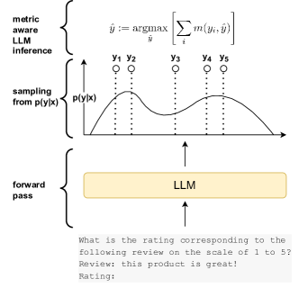
Figure 1: An illustration of the metric aware LLM inference (MBR decoding applied to regression and scoring tasks). First, an input example is passed to an LLM (forward pass). We next obtain samples from the distribution over targets conditioned on the input $x$ (sampling from $p(y\mid x)$). Finally, the obtained samples are used for finding the target optimizing a metric ${m}$ (metric aware LLM inference); see Table 1 for specific solutions corresponding to example metrics.

2 When (Naïve) LLM Inference Fails on scoring tasks

We begin by describing the problem setting. Fix a finite vocabulary $V$ of tokens (e.g., words in English). Let $D$ denote a distribution over inputs $x\in X\subseteq{V}^{*}$ comprising of strings of tokens and targets sequences $y\in Y$. Let $p(y\mid x)$ denote the conditional distribution over targets given an input.

A special case of this setting is when $Y\subset\mathbb{R}$ corresponds to numeric targets. Here, we assume that each $y\in Y$ has a unique string representation ${\tt str}(y)\in V^{*}$; for example, the integer $1$ has the string encoding "1". In a slight abuse of notation, we use $p(y\mid x)\stackrel{{\scriptstyle\cdot}}{{=}}p({\tt str}(y)\mid x)$ to denote the conditional probability of output $y$ given input $x$.

A language model (LM) takes a string $x$ as input and predicts an output $\hat{y}\in Y$. Typically, the LM first produces a distribution $\hat{p}(\cdot\mid x)$ over targets, from which a prediction is derived via a suitable inference (or decoding) procedure. Perhaps the most common inference strategy is to choose the mode of $\hat{p}(y\mid x)$:

$$\hat{y}(x):=\operatorname*{argmax}_{y\in Y}\hat{p}(y\mid x).$$ (1)

In practice, one may approximate the mode by employing greedy decoding or beam search, or sampling multiple candidates with a temperature and picking the among them the one with the highest likelihood score (Naseh et al., 2023).

The quality of an LM’s prediction is measured by some evaluation metric $m(y,\hat{y})$, where we assume that higher values are better. While the exact match (EM), given by $m(y,\hat{y})=\mathds{1}({y=\hat{y}})$, is a commonly used evaluation metric, there are a range of other metrics popularly used to evaluate LMs. These include the (negative) squared error $m(y,\hat{y})=-(y-\hat{y})^{2}$ or absolute error $m(y,\hat{y})=-|y-\hat{y}|$ in the case of numerical targets, or text-based metrics such as $F_{1}$ or BLEU.

A natural goal is to then choose the inference strategy $\hat{y}(x)$ to maximize the metric $m$ of interest, i.e., to maximize the following expected utility:

$$\mathbb{E}_{(x,y)\sim D}\left[m(y,\hat{y}(x))\right].$$ (2)

As we shall see below, for many choices of metric $m(y,\hat{y}(x))$, picking the mode of the predicted distribution (1) can be sub-optimal for (2).

Example 1.

Consider the task of predicting the star rating (on the scale $1$–$5$) associated with a review text. Suppose $m(y,\hat{y})$ is the negative absolute error between true and predicted star ratings. Given the review text ‘‘This keybord is suitable for fast typers’’, suppose the responses and the associated probabilities from an LM are {‘‘1’’: 0.3,  ‘‘2’’: 0.0,  ‘‘3’’: 0.3,  ‘‘4’’: 0.0,  ‘‘5’’: 0.4}. The mode of the predicted probabilities is ‘‘5’’. In contrast, the maximizer of (2) is the median rating ‘‘3’’. We provide real examples for Amazon reviews of learn probability distributions and the label in Figure 2 (Appendix).

Example 2.

Consider a reading comprehension task, where we use the $F_{1}$ score as the evaluation metric $m(y,\hat{y})$, defined by the harmonic mean of $\text{recall}(y,\hat{y})=\frac{|y\cap\hat{y}|}{|y|}$ and $\text{precision}(y,\hat{y})=\frac{|y\cap\hat{y}|}{|\hat{y}|}$. Suppose for the question ‘‘What is the hottest month in the year’’, the responses and associated probability from an LM are {‘‘July’’: 0.25,  ‘‘July 2023’’: 0.23,  ‘‘Month of July’’: 0.24,  ‘‘May’’: 0.28}. The mode of this distribution is ‘‘May’’; whereas the maximizer of (2) is ‘‘July’’.

3 Metric-aware LLM inference

We seek to design decoding strategies that maximize the expected utility in (2).

3.1 Minimum Bayes risk decoding

In an idealized setting, where we have access to the true conditional probabilities $p(\cdot\mid x)$, it is straight-forward to show that the maximizer of (2) is:

$$\hat{y}^{*}(x)\in\operatorname*{argmax}_{y^{\prime}\in Y}\,\mathbb{E}_{y\sim p(\cdot\mid x)}\left[m(y,y^{\prime})\right].$$ (3)

When $m$ is the EM metric, the optimal inference strategy is $\hat{y}^{*}(x)\in\operatorname*{argmax}_{y\in Y}\,p(y\mid x),$ which is what common approaches such as greedy decoding seek to approximate.

In general, however, the optimal decoding strategy can have a very different form, and a mode has been shown to be suboptimal on generation tasks (Eikema and Aziz, 2020). For example, for evaluation metrics over numerical targets such as the squared error or the absolute error, the optimal inference strategy is to simply take the mean or median of $p(\cdot|x)$ (Bishop, 2006). Table 1 summarizes these optimal rules for different metrics.

3.2 Approximating the optimal solution

In practice, we mimic the Bayes-optimal solution in (3) with two approximations. First, we replace the true conditional distribution ${p}(\cdot\mid x)$ with the LM’s predicted distribution $\hat{p}(\cdot\mid x)$. This is a reasonable approximation when the LM is pre-trained with next-token prediction task and softmax cross-entropy loss: the latter is a strictly proper loss, whose minimizer under an unrestricted hypothesis class is the true conditional distribution $p(y\mid x)$ (Gneiting and Raftery, 2007).

Second, we estimate the expectation in (3) by sampling $K$ outputs from $\hat{p}(\cdot\mid x)$ with a sampling temperature $T$, and then computing:

$$\hat{y}(x)\in\operatorname*{argmax}_{y^{\prime}\in Y}\,\sum_{i=1}^{K}m(y_{i},y^{\prime}).$$ (4)

As noted in Table 1, the above maximization can be computed in closed-form for some common metrics. In applications where we neither have a closed-form solution, nor can enumerate $S$ feasibly, we may solve (4) approximately by maximizing over a fixed subset $C\subset Y$ of candidate outputs:

$$\hat{y}(x)\in\operatorname*{argmax}_{y^{\prime}\in C}\,\sum_{i=1}^{K}m(y_{i},y^{\prime}).$$ (5)

The choice of $C$ would depend on the task and metric at hand. For example, one simple choice is for $C$ to be the $K$ sampled outputs, i.e., $C=\{y_{1},\ldots,y_{K}\}$. In Appendix A.1, we described how we choose $C$ for text generation tasks.

The quality of our inference strategy depends on the sampling temperature $T$, the number of samples $K$, and the choice of $C$. Note that sampling can be done efficiently by caching the Transformer activations for the input prefix when generating different targets; the Transformer computation needs to be repeated only for the different sampled targets.

3.3 Post-hoc temperature scaling

As mentioned, when sampling from $\hat{p}(\cdot\mid x)$, it often helps to apply a temperature scaling to the LM logits to control the diversity of the sampled outputs. This is particularly important in our procedure where we wish to approximate expectations over $\hat{p}(\cdot|x)$ using a few samples.

In practice, one may sample from $\hat{p}(\cdot\mid x)$ with temperature $T=1$, and apply temperature scaling in a post-hoc manner by employing a weighted version of the objective in (4):

$$\hat{y}(x)\in\operatorname*{argmax}_{y^{\prime}\in Y}\,\sum_{i=1}^{K}\left(\hat{p}(y_{i}\mid x)\right)^{\alpha}\cdot m(y_{i},y^{\prime}),$$ (6)

where $\alpha$ can be seen as the temperature scaling parameter. The above summation is a (scaled) estimate of $\mathbb{E}_{y\sim\hat{p}(\cdot\mid x)}\left[\hat{p}(y\mid x)^{\alpha}\cdot m(y,y^{\prime})\right]$. For probabilities $\hat{p}(y_{i}\mid x)\propto\exp(f(x,y_{i}))$ defined by logits $f(x,y_{i})$, this is equivalent to computing the expectation under the temperature-scaled distribution $\hat{p}_{\alpha}(y\mid x)\propto\exp((1+\alpha)\cdot f(x,y))$, albeit a normalization factor. We consider an analogous weighting scheme for the plug-in estimators of the closed-form solutions reported in Table 1.

Problem	Label space $Y$	Metric	Optimal decision rule
Classification	$1,\ldots,K$	$\mathds{1}({y=\hat{y}})$	$\hat{y}(x):=\operatorname*{argmax}_{y}[p(y\mid x)]$
Regression	$\mathbb{R}$	$-(y-\hat{y})^{2}$	$\hat{y}(x):=\mathbb{E}_{y\sim p(\cdot\mid x)}[y]$
Ordinal regression	$1,\ldots,K$	$-|y-\hat{y}|$	$\hat{y}(x):=\text{median}[p(\cdot\mid x)]$
Bi-partite ranking	$\pm 1$	AUC	$\hat{y}(x):=p(y=+1|x)$
Multi-partite ranking	$1,\ldots,K$	$\text{AUC}^{\text{multi}}$  with costs $c_{y,y^{\prime}}=|y-y^{\prime}|$	$\hat{y}(x):=\mathbb{E}_{y\sim p(\cdot\mid x)}[y]$
Question answering	$V^{*}$	$F_{1}(y,\hat{y})$	$\hat{y}(x):=\operatorname*{argmax}_{y^{\prime}}\,\mathbb{E}_{y\sim p(\cdot\mid x)}\left[F_{1}(y,y^{\prime})\right]$

Table 1: Optimal decision rule for different evaluation metrics. Except $F_{1}$, all metrics admit a closed-form solution. For $F_{1}$, we approximate the optimal solution by optimizing over a subset of candidates $C\subset Y$ (§3.2). See §3.5 for definitions of AUC. For the ranking problems, the LLM predicts a real-valued score, which is then used to rank the samples; for all others, the LLM predicts an output in label space $Y$.

	model size	greedy decode		MALI9in
			argmax	mean
STSB	XXS	1.078	1.448	1.028
	S	0.685	1.019	0.649
	L	0.628	0.989	0.610
			argmax	median
Amazon reviews	XXS	0.495	0.826	0.474
	S	0.301	0.444	0.285
	L	0.294	0.541	0.291
			argmax	$F_{1}$
Trivia-QA	XXS	0.314	0.178	0.302
	S	0.620	0.636	0.678
	L	0.886	0.887	0.886

Table 2: Root mean squared error (RMSE) on STSB dataset (lower is better), Mean absolute error (MAE) on Amazon reviews dataset (lower is better), and $F_{1}$ metrics on Trivia-QA dataset (higher is better) from PaLM-2 models of varying size. We sample $16$ targets for the argmax and MALI methods. All methods rely on $T=1$ temperature for sampling, and the weighted approaches correspond to an effective temperature $T=\frac{1}{4}$. See Tables 6, 7, 8 in the Appendix for results over more temperatures and evaluation metrics (cost weighted multi-class AUC and Pearson correlation).

3.4 Efficiency

Note that sampling can be done efficiently by caching the Transformer activations for the input prefix when generating different targets. The Transformer computation needs to be repeatedly done only for the different sampled targets.

In practice, when the prefix is long compared to the generated targets (e.g. for scoring tasks, where the target score can be just a few tokens length, whereas the prefix can be long as it contains the input text), a forward pass for the prefix tends to take most of the compute time.

Moreover, we generate multiple samples simultaneously, and so, we do not incur a higher cost from generating multiple targets.

3.5 Ranking metrics

Apart from the settings where evaluation metrics are decomposable, i.e., evaluation metrics are a result of aggregation of per-example results from evaluation, there are also metrics which are non-decomposable. An example for such a metric are ranking metrics, where the goal is to correctly order examples, as opposed to predict correct scores or classes. Ranking metrics are appropriate for many important tasks, including ads click-through rate prediction or recommender systems. Below we review different types of ranking metrics and the corresponding optimal decision rules.

Bi-partite ranking

In bi-partite ranking, the goal is to order examples from two classes (and so the label set $Y={\pm 1}$) in such a way that examples from the positive class are above the examples from the negative class. In this case The LLM predicts real valued scores, and so the target space need not be the same as the label space. One common metric used for evaluating bi-partite ranking is the area under the ROC curve (AUC), which is proportional to the number of wrongly ordered pairs of examples in the ranking (Cortes and Mohri, 2003):

$$\text{AUC}(\hat{y})\,=\,1-\mathbb{E}\Big{[}\mathds{1}(\hat{y}(x)<\hat{y}(x^{\prime}))\,+\,\frac{1}{2}\cdot\mathds{1}(\hat{y}(x)=\hat{y}(x^{\prime})\,\Big{|}\,y=+1,y^{\prime}=-1\Big{]}$$

It can be shown that the optimal decision rule for AUC takes the form of (any strictly monotone transformation of) $\hat{y}^{*}(x)=p(y=+1|x)$ (Clémençon et al., 2008; Uematsu and Lee, 2015).

Multi-partite ranking

Multi-partite ranking is an extension to the bi-partite ranking, where the ranking is over examples from multiple categories. Several multi-category extensions of binary AUC have been considered, for example by counting wrongly ordered pairs of examples in the ranking according to the category indices and weighing them according to predetermined costs (Uematsu and Lee, 2015):

$$\text{AUC}^{\text{multi}}(\hat{y})\,=\,1-\mathbb{E}\Big{[}c_{y,y^{\prime}}\cdot\Big{(}\mathds{1}(\hat{y}(x)<\hat{y}(x^{\prime}))\,+\,\frac{1}{2}\cdot\mathds{1}(\hat{y}(x)=\hat{y}(x^{\prime})\Big{)}\,\Big{|}\,y>y^{\prime}\Big{]}$$

Uematsu and Lee show that when the costs are equal to the difference between category indices, i.e., $c_{y,y^{\prime}}=|y-y^{\prime}|$, an optimal solution is to use mean distribution over scores: $\hat{y}^{*}(x)=\mathbb{E}_{y\sim p(\cdot|x)}\left[y\right]$. We report results on the cost weighted multi-class AUC in Table 7 in Appendix.

4 Experiments and discussion

We compare our metric-aware inference approach against standard inference strategies on NLP tasks with different evaluation metrics. 

Datasets. We summarize the datasets below, and list the prompts used in Table 5 (Appendix). 

1. STSB: The Semantic Textual Similarity Benchmark (Cer et al., 2017) comprises of sentence pairs human-annotated with a similarity score from 0 to 5. As it is a regression task, we consider evaluation with root mean squared error.

2. US Amazon reviews: We evaluate on a sample of $1500$ examples from the US Amazon reviews dataset. From the review text we aim to predict the 5-star rating corresponding to a product review (Ni et al., 2019). Since the task is in the form of ordinal regression, we use mean absolute error as the metric (Fathony et al., 2017).

3. TriviaQA is a reading comprehension dataset comprising (question, answer, reference text) triplets, where a question is answered against a refence text (Joshi et al., 2017). The evaluation is the $F_{1}$ score (see Example 2).

We use a sample of $1500$ examples for evaluation. 

Models. We consider two instruction-tuned model families: FLAN-T5 (Chung et al., 2022) and PaLM-2 (Google and et al., 2023). We report results across different model sizes and temperatures. Unless otherwise stated, we fix the number of samples to $K=16$, and the top-$k$ parameter in decoding to $40$ (Fan et al., 2018). 

Methods. We evaluate the following methods (i) greedy decoding, (ii) a baseline inspired from the self-consistency decoding of sampling $K$ candidates and picking the one with the maximum likelihood (argmax) (Wang et al., 2023a), (iii) the proposed MALI approach on the same $K$ samples, and (iv) the temperature scaled variant of MALI in §3.3 (denoted by a ‘*’). For (iv), we choose $\alpha$ so that the effective temperature is $\frac{1}{4}$. For the tasks involving the squared and absolute error metrics, we use the closed-form decision rules in Table 1. For the $F_{1}$ metric, we solve (5) over a candidate set $C$, which we choose to contain the $K$ samples and additional targets derived from them (details in Appendix A.2).  

Metric-aware inference helps. In Table 2, we report results across datasets and model sizes. We notice that MALI improves over baselines across all model sizes on STSB and Amazon reviews (for model size S, we see that median performs very similarly to the most likely generated sample). On Trivia QA, we find that on XXS and S, optimizing for $F_{1}$ helps, and for L, simply using the most likely generated sample works most effectively.

We see diminishing improvements with larger models for Trivia QA and Amazon datasets. This coincides with a lowering entropy in predictions with increasing model size for Trivia QA and Amazon datasets, whereas STSB does not exhibit this phenomenon as strongly: see Table 9 (Appendix) for empirical entropy estimates.

We also evaluate MALI with varying number of samples $K$. As seen in Table 10 (Appendix), on STSB with temperature $\frac{1}{4}$, even with as few as two samples, MALI starts to show improvements over greedy decoding. 

Sampling versus scoring. So far, when estimating the prediction maximizing the (2), we have used sampling from the LM distribution (see §3.2). Alternatively, if the targets are from a narrow interval (e.g., on the STSB dataset, the values are in the interval $[0,5]$), one can find the probabilities for targets at fixed intervals (e.g. $0,0.5,1.0,\ldots,5.0$), and thus find the solutions from Table 1 and more generally from (3).

In Table 3, we report results from FLAN-T5 on the STSB dataset for both scoring and sampling based estimates for MALI, where the scoring based estimator is based on $11$ equally spaced targets. We find that both sampling and scoring lead to MALI improving over choosing the most likely prediction. Further, we note that sampling is a more effective strategy than scoring the equally spaced targets.

model	greedy	scoring	sampling
FLAN-T5 S	4.419	2.407	2.275
FLAN-T5 L	0.455	0.410	0.373
FLAN-T5 XL	0.508	0.549	0.457

Table 3: Squared error (SE) on STSB from FLAN-T5 models of varying size. Temperature $0.5$ was used for generating targets for the sampling approach.

5 Further related work

Minimum Bayes risk decoding.

As noted in the introduction, prior work on MBR have considered optimizing for common metrics in the machine translation and text generation literature. The closest to our paper is the work of Wang et al. (2023a), who considered sampling from the model distribution when applied with chain of thought prompting, and showed how majority vote improves over the baseline under different arithmetic and reasoning tasks. Other works explored different aspects of MBR, including: the role of the sampling algorithms (Freitag et al., 2023; Cheng and Vlachos, 2023), how label smoothing interacts with MBR (Yan et al., 2022), and how it generalizes other techniques (Suzgun et al., 2022; Bertsch et al., 2023).

Finetuning approaches for target tasks alignment.

Previous works considered approaches for aligning the models for target datasets. For example, soft prompts were finetuning on target datasets without loosing generalization to other tasks (Wang et al., 2023b), and general finetuning was conducted on carefully tailored datasets for improved model robustness (Li et al., 2023). In our work, we focus on zero-shot setting where no fine-tuning is conducted.

Finetuning approaches for numerical tasks.

Autoregressive finetuning of LLMs on numerical tasks with CoT has been found effective (Liu and Low, 2023). One line of work for modeling predictive tasks with pre-trained Transformer based models is to add a regression head on top of the transformed/pooled encoded input tokens and finetune the resulting model on numerical targets using a regression loss. This is an approach which has been for encoder based models (e.g. Bert), and has also been applied to encoder-decoder (e.g. T5) models (Liu et al., 2022), and these approaches could be extended to decoder models too. In this work, we focus on the zero shot approaches, and so we leave training approaches for future work.

6 Conclusions

In this work we show how adopting MBR to regression and scoring tasks, and thus utilizing the output distribution modeled by LLMs in the form of our MALI methods can bring improvements. Our work also points at importance of further understanding and improving of the quality of model output distribution and calibration, which we found crucial for the MALI methods to work well.

7 Limitations

There are multiple limitations of our work. First, we evaluate our proposed methods on multiple text datasets with numerical and text targets, however, many more types of outputs can be considered, including time series targets, long text targets etc. Next, it would be interesting to more systematically analyze how to solve the objective from (6) over many samples for text outputs for metrics like $F_{1}$ or BLEU, e.g. by means of dynamic programming. We also note that the datasets considered in this work are restricted to English. It would be interesting to expand the explorations to datasets in other languages.

8 Ethics Statement

All datasets used in this work are publicly available. No additional user data was collected or released as part of this work. All models used are publicly available and already pretrained, and no finetuning was conducted for any experiments. Instead, all experiments relied on running inference experiments with the models over several thousands of examples. Thus, the CO-2 footprint of this paper is minimal. We do not foresee any significant risks associated with this paper other than improving performance on tasks which are harmful.

9 Acknowledgements

We are thankful to Ziwei Ji for the helpful feedback.

Appendix A Appendix

A.1 Candidate set construction

One simple choice for the candidate set $C$ could be take the $K$ sampled outputs, i.e., $C=\{y_{1},\ldots,y_{K}\}$. One may additionally include in this set transformations on each $y_{i}$ $y_{i}$ or new candidates formed from combining two or more of the samples.

For example, in applications such as reading comprehension or question-answering, where the output is list of keywords that constitute an answer to a question, one often uses a metric such as F1 that balances between precision and recall. In such cases, after sampling, one may additionally include samples formed by concatenating pairs of sampled outputs, i.e., ${\tt concat}(y_{i},{\tt delim},y_{j}),\forall i\neq j$. These concatenated answers have the effect of increasing recall, at the cost of lower precision. We follow that procedure for the Trivia-QA experiments in §4.

To analyze the effectiveness of the candidate set augmentation, in Table 4 we compare the performance of MALI (specifically the temperature scaled variant) with and without the inclusion of concatenated pairs in the candidate set. For both the XXS and S models, the inclusion of concatenated pairs is seen to yield a significant improvement in F1-score.

model	w/ pairs	w/o pairs
PaLM-2 XXS	$0.302$	$0.295$
PaLM-2 XS	$0.678$	$0.670$
PaLM-2 L	$0.886$	$0.887$

Table 4: Performance of MALI (as evaluated by $F_{1}$) on TriviaQA with and without the inclusion of concatenated pairs in the candidate set.

A.2 Additional details

In Table 5 we report the prompts we used in our experiments for zero-shot inference.

For all datasets, we use validation splits, and where not available, we use the first $1500$ examples from the train split.

The datasets are publicly available, for example from the tensorflow.org platform:

• https://www.tensorflow.org/datasets/catalog/glue#gluestsb,

• https://www.tensorflow.org/datasets/catalog/amazon_us_reviews,

• https://www.tensorflow.org/datasets/catalog/trivia_qa.

Dataset	Prompt
STSB	What is the sentence similarity between the following two sentences measured on a scale of 0 to 5: {Sentence #1}, {Sentence #2}. The similarity measured on a scale of 0 to 5 with 0 being unrelated and 5 being related is equal to
Amazon reviews	What is the rating corresponding to the following review in the scale of 1 to 5, where 1 means negative, and 5 means positive? Only give a number from 1 to 5 with no text. Review: {Review} Rating:
Trivia-QA	Answer the following question without any additional text. Question: {Question}. Answer:

Table 5: Prompts used for different datasets. Curly braces denote inputs specific to an input example.

A.3 Additional experiments

In Table 9 we report empirical entropy estimates as measured based on the $16$ samples generated from the model. We find that entropy decreases as model size increases. We observe a particularly sharp decrease in entropy for the Amazon reviews and Trivia-QA datasets, where for larger model sizes we don’t find improvements from MALI approaches.

In Table 6 we report RMSE on STSB dataset, MAE on Amazon reviews dataset, and $F_{1}$ metrics on Trivia-QA dataset from PaLM-2 models of varying size across multiple temperature values. We find improvements over baselines on STSB and Amazon reviews datasets for most temperatures. For Trivia-QA, we find improvements for XXS and S models for some temperatures, and for L, we don’t find a difference from our methods due to low entropy in the responses (see Table 9). In Table 8 we additionally report Pearson correlation metrics on STSB, confirming the results of MALI improving over autoregressive inference. Lastly, in Table 7 we report cost weighted multi-class AUC with costs corresponding to the difference between the annotated labels: $|y_{1}-y_{2}|$. We find on both STSB and Amazon reviews datasets that the optimal decision rule (mean over the distribution) improves over the baselines.

In Table 10, we report the impact of the number of samples on the results. We note that there is an improvement in the results with the increase in the number of samples, however beyond 8 samples there is a diminishing improvement in practice.

In Figure 2 we report examples from the Amazon dataset and the corresponding: human annotations and samples from the model. Notice how samples cover significant proportions of the ratings. We find that the samples end up in the vicinity of the human annotation, and thus in many cases taking a mean over samples helps improve the prediction over the mode.

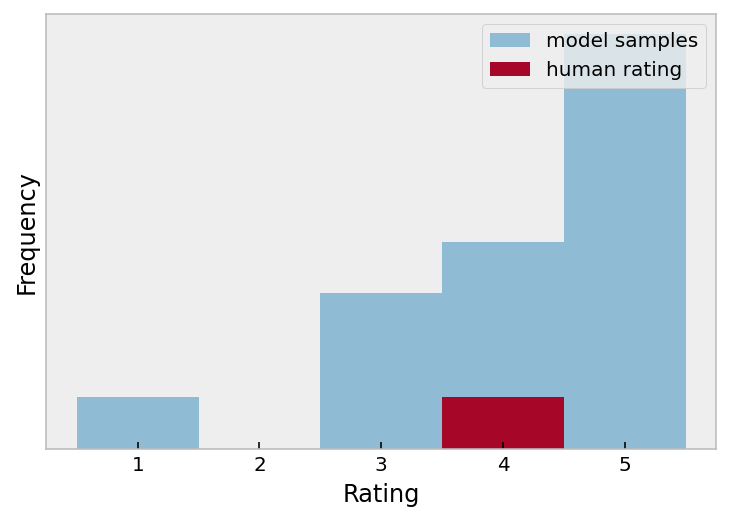
(a) It is a nice color of black and my husband likes how it feels in his hand.

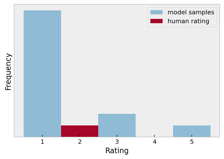
(b) This item is a good idea. However, Unless the ear canal is reasonably deep (…) it’s of no use. The plastic hooks that come with it are hard and too small (…). Might be good for children.

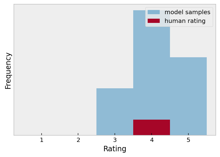
(c) One of the sides is made for apple products, the other is just standard usb. Both will work with apple products, just one side (the A side) charges faster. Other than that, it’s fantastic. :D

Figure 2: Examples from the Amazon dataset and the corresponding: human annotations and samples from the model. We find that in many cases, taking mean over model samples is closer to the annotation than taking the mode of the distribution.

	model size	greedy decode	T=$0.25$			T=$0.5$			T=$1.0$
			argmax	mean	w-mean	argmax	mean	w-mean	argmax	mean	w-mean
STSB	XXS	1.078	1.126	1.043	1.028	1.241	1.021	0.992	1.448	1.007	0.978
	S	0.685	0.787	0.643	0.649	0.908	0.636	0.642	1.019	0.641	0.641
	L	0.628	0.729	0.592	0.610	0.852	0.582	0.586	0.989	0.580	0.580
			T=$0.25$			T=$0.5$			T=$1.0$
			argmax	median	w-median	argmax	median	w-median	argmax	median	w-median
Amazon reviews	XXS	0.495	0.509	0.484	0.474	0.624	0.485	0.487	0.826	0.493	0.493
	S	0.301	0.290	0.297	0.285	0.329	0.300	0.297	0.444	0.299	0.299
	L	0.294	0.318	0.293	0.291	0.380	0.294	0.293	0.541	0.298	0.295
			T=$0.25$			T=$0.5$			T=$1.0$
			argmax	$F_{1}$	w-$F_{1}$	argmax	$F_{1}$	w-$F_{1}$	argmax	$F_{1}$	w-$F_{1}$
Trivia-QA	XXS	0.314	0.300	0.319	0.318	0.255	0.323	0.326	0.178	0.307	0.304
	S	0.620	0.656	0.626	0.678	0.658	0.641	0.662	0.636	0.650	0.650
	L	0.886	0.888	0.886	0.888	0.888	0.883	0.887	0.887	0.880	0.885

Table 6: Root mean squared error (RMSE) on STSB dataset (the lower the better), Mean absolute error (MAE) on Amazon reviews dataset (the lower the better), and $F_{1}$ metrics on Trivia-QA dataset (the higher the better) from PaLM-2 models of varying size. We report different methods of inference across different temperatures. For the weighted approaches, we fix the sampling temperature to $T=1$ and accordingly vary the $\alpha$ in (6) so as to arrive at the effective temperature equal to the value reported.

	model size	greedy decode	T=$0.25$		T=$0.5$		T=$1.0$
			argmax	mean	argmax	mean	argmax	mean
STSB	XXS	$0.797$	$0.755$	$0.882$	$0.714$	$0.890$	$0.632$	$0.889$
	XS	$0.895$	$0.870$	$0.950$	$0.843$	$0.954$	$0.820$	$0.953$
	L	$0.905$	$0.885$	$0.948$	$0.859$	$0.959$	$0.827$	$0.961$
Amazon reviews	XXS	$0.87$	$0.894$	$0.925$	$0.866$	$0.94$	$0.788$	$0.942$
	XS	$0.9$	$0.91$	$0.925$	$0.914$	$0.941$	$0.9$	$0.958$
	L	$0.925$	$0.922$	$0.951$	$0.906$	$0.962$	$0.837$	$0.964$

Table 7: Cost-weighted multi-partite AUC metrics on STSB and Amazon datasets (the higher the better). MALI methods improve over the baselines. See §3.5 for the definition of AUC we use. We assume costs to correspond to the difference between the annotated labels: $|y_{1}-y_{2}|$.

model	greedy decode	T=$0.25$		T=$0.5$		T=$1.0$
		argmax	mean	argmax	mean	argmax	mean
PaLM-2 XXS	$0.767$	0.738	$\mathbf{0.790}$	0.670	$\mathbf{0.790}$	0.544	$0.786$
PaLM-2 XS	$0.898$	0.878	$\mathbf{0.915}$	0.852	$0.913$	0.821	$0.910$
PaLM-2 L	$0.909$	0.893	$0.920$	0.881	$0.922$	0.860	$\mathbf{0.923}$

Table 8: Pearson correlation metrics on STSB. MALI methods improve over the baselines.

model	STSB	Amazon	Trivia-QA
PaLM-2 XXS	$1.141$	$1.064$	$1.328$
PaLM-2 XS	$1.055$	$0.753$	$0.475$
PaLM-2 L	$0.976$	$0.361$	$0.186$

Table 9: Empirical entropy across model sizes and datasets.

samples	XXS	S	L
(Greedy Decode)	1.078	0.685	0.628
2	1.044	0.679	0.624
4	1.036	0.669	0.613
6	1.031	0.664	0.607
8	1.028	0.660	0.603
10	1.025	0.657	0.601
12	1.024	0.655	0.600
14	1.022	0.653	0.599
16	1.021	0.652	0.598

Table 10: RMSE as a function of the number of samples on STSB across PaLM-2 models of varying size. Results for temperature $T=0.25$.

References

- Bertsch et al. (2023) Amanda Bertsch, Alex Xie, Graham Neubig, and Matthew Gormley. It’s MBR all the way down: Modern generation techniques through the lens of minimum Bayes risk. In Yanai Elazar, Allyson Ettinger, Nora Kassner, Sebastian Ruder, and Noah A. Smith, editors, Proceedings of the Big Picture Workshop, pages 108–122, Singapore, December 2023. Association for Computational Linguistics. doi: 10.18653/v1/2023.bigpicture-1.9. URL https://aclanthology.org/2023.bigpicture-1.9.
- Bishop (2006) Christopher M. Bishop. Pattern Recognition and Machine Learning (Information Science and Statistics). Springer-Verlag, Berlin, Heidelberg, 2006. ISBN 0387310738.
- Cer et al. (2017) Daniel Cer, Mona Diab, Eneko Agirre, Inigo Lopez-Gazpio, and Lucia Specia. Semeval-2017 task 1: Semantic textual similarity multilingual and crosslingual focused evaluation. In Proceedings of the 11th International Workshop on Semantic Evaluation (SemEval-2017). Association for Computational Linguistics, 2017. doi: 10.18653/v1/s17-2001. URL http://dx.doi.org/10.18653/v1/S17-2001.
- Cheng and Vlachos (2023) Julius Cheng and Andreas Vlachos. Faster minimum bayes risk decoding with confidence-based pruning. arXiv preprint arXiv:2311.14919, 2023.
- Chung et al. (2022) Hyung Won Chung, Le Hou, Shayne Longpre, Barret Zoph, Yi Tay, William Fedus, Yunxuan Li, Xuezhi Wang, Mostafa Dehghani, Siddhartha Brahma, Albert Webson, Shixiang Shane Gu, Zhuyun Dai, Mirac Suzgun, Xinyun Chen, Aakanksha Chowdhery, Alex Castro-Ros, Marie Pellat, Kevin Robinson, Dasha Valter, Sharan Narang, Gaurav Mishra, Adams Yu, Vincent Zhao, Yanping Huang, Andrew Dai, Hongkun Yu, Slav Petrov, Ed H. Chi, Jeff Dean, Jacob Devlin, Adam Roberts, Denny Zhou, Quoc V. Le, and Jason Wei. Scaling instruction-finetuned language models, 2022.
- Clémençon et al. (2008) Stéphan Clémençon, Gábor Lugosi, and Nicolas Vayatis. Ranking and empirical minimization of u-statistics. The Annals of Statistics, 36(2):844–874, 2008. ISSN 00905364. URL http://www.jstor.org/stable/25464648.
- Cortes and Mohri (2003) Corinna Cortes and Mehryar Mohri. Auc optimization vs. error rate minimization. In S. Thrun, L. Saul, and B. Schölkopf, editors, Advances in Neural Information Processing Systems, volume 16. MIT Press, 2003. URL https://proceedings.neurips.cc/paper_files/paper/2003/file/6ef80bb237adf4b6f77d0700e1255907-Paper.pdf.
- Eikema and Aziz (2020) Bryan Eikema and Wilker Aziz. Is MAP decoding all you need? the inadequacy of the mode in neural machine translation. In Donia Scott, Nuria Bel, and Chengqing Zong, editors, Proceedings of the 28th International Conference on Computational Linguistics, pages 4506–4520, Barcelona, Spain (Online), December 2020. International Committee on Computational Linguistics. doi: 10.18653/v1/2020.coling-main.398. URL https://aclanthology.org/2020.coling-main.398.
- Eikema and Aziz (2022) Bryan Eikema and Wilker Aziz. Sampling-based approximations to minimum Bayes risk decoding for neural machine translation. In Yoav Goldberg, Zornitsa Kozareva, and Yue Zhang, editors, Proceedings of the 2022 Conference on Empirical Methods in Natural Language Processing, pages 10978–10993, Abu Dhabi, United Arab Emirates, December 2022. Association for Computational Linguistics. doi: 10.18653/v1/2022.emnlp-main.754. URL https://aclanthology.org/2022.emnlp-main.754.
- Fan et al. (2018) Angela Fan, Mike Lewis, and Yann Dauphin. Hierarchical neural story generation, 2018.
- Fathony et al. (2017) Rizal Fathony, Mohammad Ali Bashiri, and Brian Ziebart. Adversarial surrogate losses for ordinal regression. In I. Guyon, U. Von Luxburg, S. Bengio, H. Wallach, R. Fergus, S. Vishwanathan, and R. Garnett, editors, Advances in Neural Information Processing Systems, volume 30. Curran Associates, Inc., 2017. URL https://proceedings.neurips.cc/paper_files/paper/2017/file/c86a7ee3d8ef0b551ed58e354a836f2b-Paper.pdf.
- Freitag et al. (2023) Markus Freitag, Behrooz Ghorbani, and Patrick Fernandes. Epsilon sampling rocks: Investigating sampling strategies for minimum Bayes risk decoding for machine translation. In Houda Bouamor, Juan Pino, and Kalika Bali, editors, Findings of the Association for Computational Linguistics: EMNLP 2023, pages 9198–9209, Singapore, December 2023. Association for Computational Linguistics. doi: 10.18653/v1/2023.findings-emnlp.617. URL https://aclanthology.org/2023.findings-emnlp.617.
- Ganesan (2018) Kavita Ganesan. Rouge 2.0: Updated and improved measures for evaluation of summarization tasks, 2018.
- Gemini Team and et al. (2023) Gemini Team and Rohan Anil et al. Gemini: A family of highly capable multimodal models, 2023.
- Gneiting and Raftery (2007) Tilmann Gneiting and Adrian E Raftery. Strictly proper scoring rules, prediction, and estimation. Journal of the American Statistical Association, 102(477):359–378, 2007. doi: 10.1198/016214506000001437. URL https://doi.org/10.1198/016214506000001437.
- Google and et al. (2023) Google and Rohan Anil et al. Palm 2 technical report, 2023.
- Gruver et al. (2023) Nate Gruver, Marc Finzi, Shikai Qiu, and Andrew Gordon Wilson. Large language models are zero-shot time series forecasters, 2023.
- Joshi et al. (2017) Mandar Joshi, Eunsol Choi, Daniel Weld, and Luke Zettlemoyer. TriviaQA: A large scale distantly supervised challenge dataset for reading comprehension. In Proceedings of the 55th Annual Meeting of the Association for Computational Linguistics (Volume 1: Long Papers), pages 1601–1611, Vancouver, Canada, July 2017. Association for Computational Linguistics. doi: 10.18653/v1/P17-1147. URL https://aclanthology.org/P17-1147.
- Kojima et al. (2023) Takeshi Kojima, Shixiang Shane Gu, Machel Reid, Yutaka Matsuo, and Yusuke Iwasawa. Large language models are zero-shot reasoners, 2023.
- Kumar and Byrne (2004) Shankar Kumar and William Byrne. Minimum Bayes-risk decoding for statistical machine translation. In Proceedings of the Human Language Technology Conference of the North American Chapter of the Association for Computational Linguistics: HLT-NAACL 2004, pages 169–176, Boston, Massachusetts, USA, May 2 - May 7 2004. Association for Computational Linguistics. URL https://aclanthology.org/N04-1022.
- Li et al. (2023) Daliang Li, Ankit Singh Rawat, Manzil Zaheer, Xin Wang, Michal Lukasik, Andreas Veit, Felix Yu, and Sanjiv Kumar. Large language models with controllable working memory. In Anna Rogers, Jordan Boyd-Graber, and Naoaki Okazaki, editors, Findings of the Association for Computational Linguistics: ACL 2023, pages 1774–1793, Toronto, Canada, July 2023. Association for Computational Linguistics. doi: 10.18653/v1/2023.findings-acl.112. URL https://aclanthology.org/2023.findings-acl.112.
- Liu et al. (2022) Frederick Liu, Terry Huang, Shihang Lyu, Siamak Shakeri, Hongkun Yu, and Jing Li. Enct5: A framework for fine-tuning t5 as non-autoregressive models, 2022.
- Liu and Low (2023) Tiedong Liu and Bryan Kian Hsiang Low. Goat: Fine-tuned llama outperforms gpt-4 on arithmetic tasks, 2023.
- Lukasik et al. (2020) Michal Lukasik, Boris Dadachev, Kishore Papineni, and Gonçalo Simões. Text segmentation by cross segment attention. In Bonnie Webber, Trevor Cohn, Yulan He, and Yang Liu, editors, Proceedings of the 2020 Conference on Empirical Methods in Natural Language Processing (EMNLP), pages 4707–4716, Online, November 2020. Association for Computational Linguistics. doi: 10.18653/v1/2020.emnlp-main.380. URL https://aclanthology.org/2020.emnlp-main.380.
- Naseh et al. (2023) Ali Naseh, Kalpesh Krishna, Mohit Iyyer, and Amir Houmansadr. Stealing the decoding algorithms of language models. In Proceedings of the 2023 ACM SIGSAC Conference on Computer and Communications Security, CCS ’23, page 1835–1849, New York, NY, USA, 2023. Association for Computing Machinery. ISBN 9798400700507. doi: 10.1145/3576915.3616652. URL https://doi.org/10.1145/3576915.3616652.
- Ni et al. (2019) Jianmo Ni, Jiacheng Li, and Julian McAuley. Justifying recommendations using distantly-labeled reviews and fine-grained aspects. In Kentaro Inui, Jing Jiang, Vincent Ng, and Xiaojun Wan, editors, Proceedings of the 2019 Conference on Empirical Methods in Natural Language Processing and the 9th International Joint Conference on Natural Language Processing (EMNLP-IJCNLP), pages 188–197, Hong Kong, China, November 2019. Association for Computational Linguistics. doi: 10.18653/v1/D19-1018. URL https://aclanthology.org/D19-1018.
- OpenAI et al. (2023) OpenAI et al. Gpt-4 technical report, 2023.
- Papineni et al. (2002) Kishore Papineni, Salim Roukos, Todd Ward, and Wei-Jing Zhu. Bleu: a method for automatic evaluation of machine translation. In Proceedings of the 40th annual meeting on association for computational linguistics, pages 311–318. Association for Computational Linguistics, 2002.
- Qin et al. (2023) Zhen Qin, Rolf Jagerman, Kai Hui, Honglei Zhuang, Junru Wu, Jiaming Shen, Tianqi Liu, Jialu Liu, Donald Metzler, Xuanhui Wang, and Michael Bendersky. Large language models are effective text rankers with pairwise ranking prompting, 2023.
- Schaeffer et al. (2023) Rylan Schaeffer, Brando Miranda, and Sanmi Koyejo. Are emergent abilities of large language models a mirage? In Thirty-seventh Conference on Neural Information Processing Systems, 2023. URL https://openreview.net/forum?id=ITw9edRDlD.
- Suzgun et al. (2022) Mirac Suzgun, Luke Melas-Kyriazi, and Dan Jurafsky. Follow the wisdom of the crowd: Effective text generation via minimum bayes risk decoding. arXiv preprint arXiv:2211.07634, 2022.
- Touvron et al. (2023) Hugo Touvron, Thibaut Lavril, Gautier Izacard, Xavier Martinet, Marie-Anne Lachaux, Timothée Lacroix, Baptiste Rozière, Naman Goyal, Eric Hambro, Faisal Azhar, Aurelien Rodriguez, Armand Joulin, Edouard Grave, and Guillaume Lample. Llama: Open and efficient foundation language models, 2023.
- Uematsu and Lee (2015) Kazuki Uematsu and Yoonkyung Lee. Statistical optimality in multipartite ranking and ordinal regression. IEEE Transactions on Pattern Analysis and Machine Intelligence, 37(5):1080–1094, 2015. doi: 10.1109/TPAMI.2014.2360397.
- Wang et al. (2023a) Xuezhi Wang, Jason Wei, Dale Schuurmans, Quoc V Le, Ed H. Chi, Sharan Narang, Aakanksha Chowdhery, and Denny Zhou. Self-consistency improves chain of thought reasoning in language models. In The Eleventh International Conference on Learning Representations, 2023a. URL https://openreview.net/forum?id=1PL1NIMMrw.
- Wang et al. (2023b) Yihan Wang, Si Si, Daliang Li, Michal Lukasik, Felix Yu, Cho-Jui Hsieh, Inderjit S Dhillon, and Sanjiv Kumar. Two-stage llm fine-tuning with less specialization and more generalization, 2023b.
- Wei et al. (2022) Jason Wei, Maarten Bosma, Vincent Zhao, Kelvin Guu, Adams Wei Yu, Brian Lester, Nan Du, Andrew M. Dai, and Quoc V Le. Finetuned language models are zero-shot learners. In International Conference on Learning Representations, 2022. URL https://openreview.net/forum?id=gEZrGCozdqR.
- Yan et al. (2022) Jianhao Yan, Jin Xu, Fandong Meng, Jie Zhou, and Yue Zhang. Dc-mbr: Distributional cooling for minimum bayesian risk decoding. arXiv preprint arXiv:2212.04205, 2022.
- Yang et al. (2023) Zhen Yang, Ming Ding, Qingsong Lv, Zhihuan Jiang, Zehai He, Yuyi Guo, Jinfeng Bai, and Jie Tang. Gpt can solve mathematical problems without a calculator, 2023.