RATSF: Empowering Customer Service Volume Management through Retrieval-Augmented Time-Series Forecasting

Abstract

An efficient customer service management system hinges on precise forecasting of service volume. In this scenario, where data non-stationarity is pronounced, successful forecasting heavily relies on identifying and leveraging similar historical data rather than merely summarizing periodic patterns. Existing models based on RNN or Transformer architectures often struggle with this flexible and effective utilization. To address this challenge, we propose an efficient and adaptable cross-attention module termed RACA, which effectively leverages historical segments in forecasting task, and we devised a precise representation scheme for querying historical sequences, coupled with the design of a knowledge repository. These critical components collectively form our Retrieval-Augmented Temporal Sequence Forecasting framework (RATSF). RATSF not only significantly enhances performance in the context of Fliggy hotel service volume forecasting but, more crucially, can be seamlessly integrated into other Transformer-based time-series forecasting models across various application scenarios. Extensive experimentation has validated the effectiveness and generalizability of this system design across multiple diverse contexts.

1 Introduction

At the heart of customer service volume management lies the accurate estimation of total service demand, which significantly impacts system costs. For every underestimation of 100 service requests, there is a need to urgently mobilize and supplement service staff at a cost equivalent to three times the single-unit labor cost; conversely, overestimating by 100 requests results in a waste of that same single-unit labor cost. Service volume forecasting for the Travel industry is particularly intricate because of its inherent interconnections with numerous variables, including order statuses, weather variations, international developments, and destination country policies. These factors contribute to highly non-stationary data patterns that, in turn, can lead to considerable biases when employing traditional uni-variate time series forecasting methods [9, 1, 23] which rely on period summaries and trend analyses.

In fact, across domains like stock market analysis and station traffic forecasting where business cycles and fluctuations play a significant role, there is a shared desire for a universal and flexible time series forecasting system design that can adeptly utilize historical sequence information to tackle intricate prediction challenges. Meanwhile, in the realm of time series forecasting(TSF), where models, whether based on Recurrent Neural Networks (RNNs) or Transformer, commonly face difficulties efficiently processing and extracting insights from vast amounts of historical data.

One naive way to solve this is to try elongating the sequence that the transformer processes. Some approach involves sampling historical data to fit within a limited context window. Specifically, the Informer [32] algorithm samples K points from the sequence and derives a shorter Q sequence based on these sampled points. However, this approach assumes that all historical information is equally important, which may not be suitable for many time series scenarios where different data points can carry varying significance. Perceiver [10] and similar methods opt for a different approach by mapping Query sequences to fixed lengths, reducing computation and allowing for more historical data storage. Nonetheless, they still face challenges in efficiently extracting and interpreting critical information from extended time series.

In the field of natural language processing, strides have been made to expand Transformer models’ context handling. On one front, techniques like flash-attention [5] enhance efficiency and reduce complexity, enabling longer context processing. However, it’s crucial to note that directly extending receptive fields may cause larger models to overlook significant details in lengthy inputs, like [15] mentioned.

On another front, Retrieval-Augmented Generation (RAG)-like methods have drawn attention for enhancing model performance by incorporating external information. NVIDIA’s [2] research indicates that even when models already handle large context windows in text tasks, they can still achieve substantial performance gains by retrieving and using relevant data from external sources.

Employing the concept of RAG, we have identified a potential approach. We can build a knowledge base that encompasses all historical time series, and pinpoint and utilize the most predictive historical segments with an improved transformer model, thereby refining forecast accuracy. To accomplish these, we focused on implementing three central enhancements: a knowledge base schema for efficiently indexing historical data, a cross-attention module to integrate historical information, and a predictive embedding for retrieval purposes.

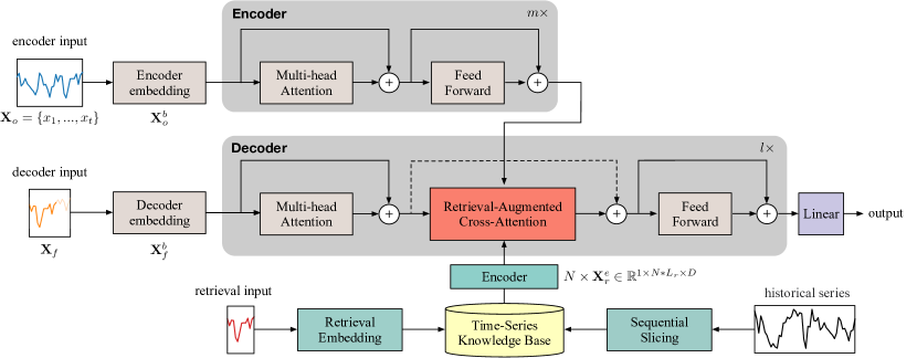
Figure 1: RATSF uses a TSKB to store and index historical sequences, alongside a transformer-based forecasting model. As illustrated in the bottom-right corner, TSKB segments the full history for efficient retrieval. To do forecasting, the Encoder fetches $\mathbf{X}_{o}$ from t recent time steps, and forms a retrieval sequence with d latest steps, retrieves N related sequences $\mathbf{X}_{r}$ from the TSKB. RACA in the Decoder then merges $\mathbf{X}_{r}$ and $\mathbf{X}_{o}$ info to deliver result.

In concise terms, our main contributions are:

1. We offer a general retrieval-augmented time-series forecasting strategy, RATSF, that can be implemented across a variety of Transformer models and their derivatives to enhance performance.

2. We employ a novel embedding strategy for precise historical piece retrieving.

3. We present a straightforward and manageable design for a time-series knowledge base, which significantly facilitates efficient management of historical data.

4. The method presented in this work currently serves as the operational algorithm for Fliggy’s service volume management system across all business domains, supporting not only hotel online bookings but also support businesses such as visa processing, flight and train ticket reservations, as well as entrance tickets to resort areas. Our method has demonstrated exceptional effectiveness in various practical application scenarios.

2 Review

Despite intense competition [20, 6, 30, 8], Transformer models [25] and their improved variants [19, 26, 16, 13, 14] have become the mainstream choice in time-series forecasting tasks. However, the computational complexity of the original Transformer model scales as O(n²) with respect to sequence length, significantly limiting the maximum sequence length it can handle and thereby constraining its ability to use historical data.

Improvements in Time-Series Forecasting with Transformers. Numbers of works focus on enhancing the Transformer model’s capability to extract temporal features, thereby improving prediction accuracy, exemplified by Fedformer’s [33] introduction of a frequency-augmented Attention mechanism that directly incorporates Fourier operators, a similar path taken by TimesNet [27]. In contrast, Autoformer [28] proposes an operator that decomposes time series information into trend and periodic components. These two types of solutions perform well for relatively stationary sequences but may see performance drop when dealing with highly non-stationary time series data.

Another core strategy involves learning a robust representation of the time series first, which is then used to enhance the forecasting accuracy. TNC [24] harnesses the core concept of contrastive learning and employs samples within a specific temporal neighborhood within a window as positive pairs, while treating samples from differing temporal neighborhoods as negative pairs. Despite these improvements having collectively boosted the ability of Transformers in time-series forecasting tasks, none has fundamentally increased the Transformer’s receptive field.

Retrieve Augmented Method in NLP. In last two years, the Retrieval-Augmented Generation (RAG) approach [7, 4, 18, 31, 21, 12, 34] has gained widespread adoption in the field of NLP. REALM harnesses a knowledge retriever to distill information from vast corpora and thereby enhance the performance of pre-trained language models. Transformer-XL+kNN [3] incorporates a K-Nearest Neighbors algorithm to search through training data, refining dialogue generation capabilities. In the context of named entity recognition tasks, U-RaNER [22] utilizes multi-modal heterogeneous retrieval techniques to boost knowledge retrive and, by integrating retrieved knowledge into the model, strengthens its understanding of queries and improves entity recognition accuracy.

Retrieval Augmented Method in Time-series Forecasting. MQ-ReTCNN [29] is designed for complex time series prediction tasks involving multiple entities and variables. It employs a scoring function to compile relevant contexts from offline data, selects scored segments, and appends them to the prediction sequence.Its retrieval mechanism emphasizes leveraging historical sequences of one entity to enhance predictions about another, without directly utilizing historical data for direct prediction assistance.

ReTime [11] creates a relation graph based on temporal closeness between sequences and employs relational retrieval instead of content-based retrieval.It does not optimally use historically similar sequences as reference points due to its inherent design limitations. Both MQ-ReTCNN and ReTime incorporate retrieval enhancement strategies but have yet to introduce a general and efficient retrieval technique specifically for single-variable time series prediction scenarios.

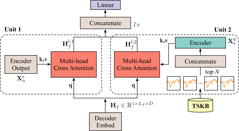
Figure 2: Each RACA has two cross-attention modules: one utilizes the Encoder output as K,V, while the other employs embedded retrieved sequences as K,V. Both outputs are concatenated and passed through a Linear module to reshape back to the input dimensions.

3 Method

Subsequently, we first provide an overview of the RATSF’s overall structure and then examine the key features of each component in detail.

The simplest description of RATSF is to first build a TSKB and then retrieve relevant sequences from it to enhance the forecasting model. For a Time Series Forecasting (TSF) task within a specific context, we first construct a TSKB using the schema detailed in Section 3.2. Next, we utilize a retrieval method to gather relevant sequences, with this method being introduced in Section 3.3. Finally, we integrate these retrieved sequences into the forecasting model, with its core computational component, RACA, being introduced in Section 3.1. Figure 1 shows the data flow of RATSF.

3.1 RACA

As previously mentioned, Retrieval-Augmented Cross-Attention (RACA) is a module designed to be plugged-into a time-series forecasting model. In our demonstration, we employ the vanilla Transformer as the time-series forecasting model; however, it’s important to note that the RACA module is designed to be compatible and can be seamlessly plug into any transformer-based time-series model.

we now provide an explanation of the abbreviations represented by subscript and superscript symbols in the following paragraphs: The letter ’o’ for original, represents the input time-series piece entering the encoder; letter ’b’ for embedding , letter ’e’ for encoder; letter ’r’ for retrieved sequence, letter ’f’ for sequence for forecasting; ’l’ for layer ; ’D’ for hidden dimension.

In transformer architecture, an encoder consists of an embedding module and multiple self-attention modules. Initially, the raw time series data $\mathbf{X}_{o}=\left\{x_{1},...,x_{t}\right\}$, $\mathbf{X}_{o}$ when processed through the embedding module, generates an output as the $\mathbf{X}^{b}_{o}$; subsequently, the output resulting from all the encoder calculation is referred as the $\mathbf{X}^{e}_{o}$.

RACA is introduced within the decoder part: besides conventionally utilizing the encoder output and the place holding embedding for the forecasting sequence, it incorporates information from N most relevant history sequences retrieved from TSKB. Like shown in Figure 2, these retrieved sequences are transformed through the encoder’s embedding module, generating Ns $\mathbf{X}^{e}_{r}$ , and we concatenate these N vectors into one with shape$[1,N*L_{r},D]$ for later use.

In Transformer-based time series forecasting models, placeholders are embedded into a $[1,L_{f},D]$ matrix, $\mathbf{H}_{f}$. The decoder consists of $l$ stacked RACA modules for inputs of length $L_{f}$. Each module has two parallel units: Unit 1, like in Function (1), uses $\mathbf{H}_{f}$ as Query with Key and Value from $\mathbf{X}^{e}_{o}$, outputting $\mathbf{H}^{l,1}_{f}$ of the same shape. Unit 2, retrieval-augment part, like in Function (2) ,also queries $\mathbf{H}_{f}$ but fetches Keys and Values from the concatenated sequence of $\mathbf{X}^{b}_{r}$, generating $\mathbf{H}^{l,2}_{f}$. $s$ in the Functions is the scaling factor.

$$\mathbf{H}^{l,1}_{f}=\text{softmax}\left(\frac{\mathbf{H}_{f}\mathbf{X}^{e}_{o}}{s}\right)\mathbf{X}^{e}_{o},$$ (1)

$$\mathbf{H}^{l,2}_{f}=\text{softmax}\left(\frac{\mathbf{H}_{f}\mathbf{X}^{e}_{r}}{s}\right)\mathbf{X}^{e}_{r},$$ (2)

$$\mathbf{H}^{l+1}_{f}=\delta\left(\text{concat}\left(\mathbf{H}^{l,1}_{f},\mathbf{H}^{l,2}_{f}\right)\right).$$ (3)

As shown in Function 3, after concatenating both intermediate vectors,$\mathbf{H}^{l,1}_{f}$ and $\mathbf{H}^{l,2}_{f}$, along the sequence dimension, forms a $[1,2*L_{f},D]$ vector, it undergoes linear transformation before being passed to the next layer.

3.2 TSKB

In the development of TSKB, we employ an innovative strategy for constructing the indexing sequence (K) and content sequence (V). Unlike traditional methods that solely store and retrieve the entire original sequence, TSKB preserves the original sequence as the core content while selects certain segments from it to construct a discriminative indexing sequence. This approach can be likened to processing a written piece where conventional methods involve direct full-text searches for desired information, which may be inefficient and less precise; whereas with TSKB, it’s akin to extracting key headlines from the body of the text to serve as indices that facilitate rapid access to core information. This dual-sequence structure allows the system, when handling large-scale data, to efficiently locate and access targeted portions of the original sequence through customized index sequences, thereby significantly enhancing overall performance.

In this article, to illustrate our system design, we employ a fixed slicing logic to select segments from V for computing the retrieval representation. In section 3.3, we will present in detail how the representation of V is learned.

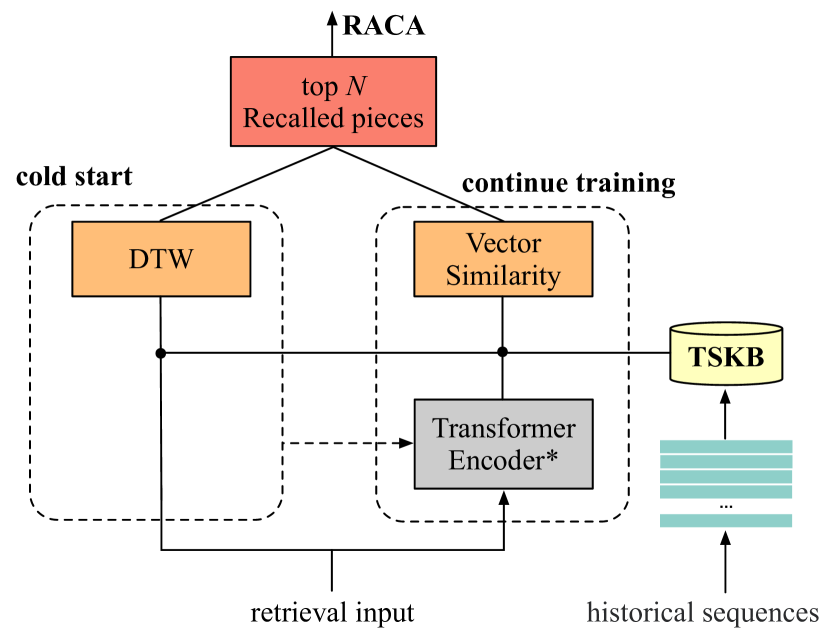
Figure 3: Within the cold start stage, we use raw sequence of retrieval input to find Top-K relevant sequences using DTW. After one epoch, we switch to Euclidean Distance for retrieval embedding to gather Top-K matches.

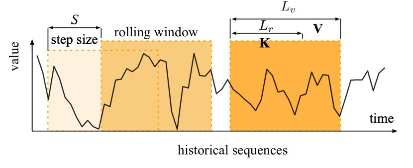
Figure 4: TSKB utilizes a rolling window of length $L_{v}$ to collect V, with an indexing segment of length $L_{r}$ taken from its leading part as K , and advances the window in steps of size S.

3.3 Learning Retrieval Embedding

Judging the quality of a retrieval representation mainly depends on how well it captures similarities at key information points relevant to forecasting tasks. Time series data is complex due to numerous information points and the challenge of presetting comparative weights. Therefore, we use this principle: if a representation closely mirrors the important details needed for prediction, its overall performance will be better. Later, we’ll explain the exact steps to put this principle into practice. We acquire the retrieval embedding for TSKB through two procedures.

3.3.1 Sequential Slicing

To obtain content sequence V, we utilize a rolling window approach where the step size is $S$ and the window length is $L_{v}$, to sample all historical sequences and incorporate them into TSKB. Since prediction models only use present data to infer the future, we align indexing sequence K with this constraint. We extract the initial segment of each V, having a length of $L_{r}$, to serve as its K. The selection of $L_{v}$, $L_{r}$ and $S$ is introduced in section 4.

3.3.2 Embedding Learning

To guarantee the embedding in capturing the essential information for forecasting, we utilize the encoder of the RATSF’s forecasting model. The model inherently excels at selecting precise information during training to improve forecast accuracy. In practice, every indexing sequence K from the knowledge base undergoes the RATSF forecasting model’s encoder layer to generate a retrieve embedding.

Meanwhile, in the early stages of training the forecasting model, its encoder is not yet capable of producing representations that accurately match target sequences. The effectiveness and learning pace of the RATSF’s forecasting model are significantly correlated with whether or not it retrieves historical sequences that are beneficial to the forecasting task.

To avoid time and data-consuming iterations stemming from a random initialization state, we introduce DTW as an auxiliary tool during the initial phase of model training, as shown in left part of Figure 3. Initially, DTW is utilized for similarity-based sequence retrieval, which is then incorporated into the iterative training process of the RATSF forecasting model. After finish one epoch of training, we transition to using embedding generated by the forecasting model itself for similar sequence retrieval, continuing the training until the model converges.

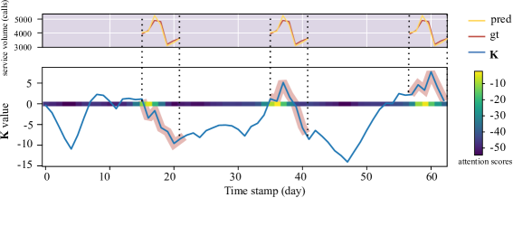
Figure 5: The lower plot displays the top 3 relevant retrieved sequences for one sample that are end-to-end connected. Each retrieved sequence has a length of 21 ($L_{f}$), comprising 14 points preceding the forecasting date and 7 points to be forecasted, highlighted with an orange background. The color bars represent aggregated cross-attention values at the first forecasting point, in which lighter color indicate higher attention value. In the upper part of the figure, predicted (yellow) and ground truth (orange) values align at corresponding positions with retrieved sequence. For this sample, the model notably focuses on segments indicating ascent and predicts a subsequent increase in value.

Table 1: Performance comparison of four Transformer models with and without the application of RATSF on three experimental datasets. All results are evaluated using MSE (Mean Squared Error) and MAE (Mean Absolute Error), and the best result is bolded.

models		transformer		nstransformer		autoformer		fedformer
metric		mse	mae	mse	mae	mse	mae	mse	mae
FHSV	baseline	4344450.512	1349.146	4414326.000	1242.128	6096673.500	1752.798	5517485.000	1638.275
	RATSF	3421546.027	1101.172	3823635.000	1070.933	5597297.500	1657.561	5386818.500	1595.657
ETTh1	baseline	3.187	1.391	1.501	0.920	8.651	2.264	4.159	1.597
	RATSF	2.366	1.180	1.407	0.886	7.300	2.113	3.952	1.565
Exchange	baseline	0.00165	0.03134	0.00014	0.00922	0.00058	0.01906	0.00172	0.03493
	RATSF	0.00068	0.02012	0.00013	0.00912	0.00067	0.02000	0.00068	0.02084

4 Experiments

In order to evaluate the generalizability and efficacy of RATSF in industry applications, we initially carry out a range of experiments to contrast the performance changes among typical time-series models when augmented with RATSF across various tasks, focusing particularly on the Fliggy Hotel Service Volume Dataset (FHSV). Following this, we employ a sequence of ablation studies to separately demonstrate the design choice of each improvement – RACA, TSKB, and Retrieval Embedding.

4.1 Experiment Setup

Datasets. Given that our primary focus lies in the forecasting task within the context of customer service volume management, we initially employed the Fliggy Hotel Service Volume Dataset to substantiate the efficacy of RATSF, the detail description of the dataset is in Appendix A. Additionally, to demonstrate the performance of our approach in other contexts, we employed two classic datasets: ETT and Exchange.

Models.We contrasted the vanilla Transformer against three of its prominent time-series domain variants: Fedformer, Autoformer, and NS-Transformer. Specifically, in keeping with the intrinsic sequential decomposition characteristics of Fedformer and Autoformer, historical segments were initially broken down using each model’s native calculations, for example the seasonal init and trend-cyclical init in Autoformer. Subsequently, these decomposed segments were embedded and fed into the RACA module for further processing.

Forecasting Setting.Consistent with the original intent of validating the effectiveness of RATSF in the context of customer service volume management, we adopt the business setting from Fliggy. In the Fliggy’s practical operations, we are required to finalize our forecasting for the upcoming week’s day-by-day staffing needs one week in advance, which is why the actual prediction window period is set at 7 days, represented as 7 tokens. In the travel industry, which Fliggy App’s serving, a quarter generally defines a relatively complete business trend. Therefore, we choose an encoder window length of 98 days—exceeding 90 days and divisible by 14—which consequently results in $\mathbf{X_{o}}$ is 98 units long. And we concate $\left\{x_{t-14},...,x_{t}\right\}$ with a placeholder of length 7 to form $\mathbf{X_{f}}$. To match the length of $\mathbf{X_{f}}$, we set $L_{v}$=21 and $L_{r}$=14. Regarding normalization, we employ unified $\mu$ and $\sigma$ values for whitening operations during the preprocessing stage and inverse normalization is carried out after forecasting. We have applied the same data processing scheme to both the ETT and Exchange datasets.

Training Setting.We have selected the Adam optimizer, with the batch size$=$64 and max training epochs$=$10. The initial learning rate (lr) is set to 0.0001, employing a linear decay strategy where the decay parameter for the first 5 epochs is 0.9, for the last 5 epochs is 0.5. We also incorporate $L1$ regularization with $\lambda$=0.0001. Concurrently, an early stopping mechanism is activated when the loss ceases to decrease.

Metric.To ensure that our evaluation metrics directly reflect business performance, we first inverse normalize the forecast result as above mentioned and then compute the MSE (Mean Squared Error) and MAE (Mean Absolute Error) against the Ground Truth. The lower these two indicators are, the more accurate the prediction results prove to be. Moreover, each decrement of 1 unit in MAE signifies a corresponding reduction of 1 unit in service staff management expenditure. This configuration has been applied uniformly across all experiments.

4.2 Main Restult

Table 1 presents the performance comparison of four Transformer models with and without the application of RATSF on three experimental datasets. In the scenario of forecasting with the Fliggy Hotel Customer Service Volume Dataset, the Transformer model’s MAE loss dropped by 18% after incorporating RATSF, potentially translating to a reduction of approximately 200 redundant personnel cost in practical management operations. Notably, even with the NSTransformer [17], Autoformer, and FedFormer models, which have undergone temporal optimization in their attention operators, adopted the RATSF design, they respectively recorded decreases in MAE loss by 14%, 5%, and 4%.

Furthermore, cross-comparison reveals that Autoformer and FedFormer yield slightly inferior results compared to the Transformer, mainly due to the stronger non-stationarity inherent in customer service volumes data within the hotel industry. As an illustrative example, while Mondays typically exhibit similar cyclical characteristics, actual service volume during Mondays preceding a short holiday can surge significantly compared to regular ones. In such instances, historical data from periods close to other short holidays provide more valuable insights than simple temporal periodicity and short-term trends; specific case studies will be showcased later.

Additionally, across the ETT and Exchange datasets, the adoption of RATSF design in the Transformer and its time-series optimized variants led to noticeable reductions in MSE metrics. Moreover, among these, the NSTransformer consistently outperforms the other models, likely because its mean-adapted feature proves effective in a broad range of time-series prediction domains.

4.3 Ablation Study

Section 4.3.1 comparatively analyzes the differences in various designs for integrating historical pieces into forecasting. Section 4.3.2 examines the impact of integrating varying numbers of historical pieces on forecast effectiveness. Section 4.3.3 demonstrates the advantages of utilizing model encoder for recalling historical pieces.

Table 2: Ablation of the specifically designed structures within RACA on FHSV scenario.

dataset	methods	metric
		mse	4344450.512
	baseline	mae	1349.146
	baseline +	mse	4071384.75
	enhanced encoder	mae	1226.850
		mse	3421546.027
FHSV	baseline + RACA	mae	1101.172

4.3.1 RACA’s design choice

Based on the Transformer architecture, two designs are considered for integrating historical pieces into the forecasting model: Design One represents a straightforward approach where historical pieces are combined with the forecasting context inputs within the encoder; Design Two employs our advanced RACA design that integrate historical pieces using cross-attention mechanisms within the decoder.

With the Fliggy Hotel Service Volume Dataset, we contrasted the performance of three methods: No historical pieces used(baseline experiment), Strategy One, and Strategy Two (RACA). The outcomes in Table 2 demonstrate that the RACA design excels, with its MAE notably lower than both the baseline and Strategy One.

A deeper examination disclosed that the Cross Attention mechanism in the RACA design efficiently guides the forecast sequence to concentrate on past trends analogous to the current scenario. Figure 5 illustrates the attention map within the RACA for the data points under forecast, where highlighted color blocks indicate that the data point being forecast places significant attention on historical segments that exhibiting similar trend patterns, and these historical segments’ trends closely align with the actual waveform following the data point in the ground truth.

4.3.2 Optimal Retrieval Count

Table 3: Results of recalling different numbers of pieces in our RATSF model.

dataset	methods	metric
		mse	4344450.512
FHSV	baseline	mae	1349.146
		mse	3678230.020
	recalled Top-1 pieces	mae	1160.101
		mse	3700934.754
	recalled Top-2 pieces	mae	1155.952
		mse	3421546.027
	recalled Top-3 pieces	mae	1101.172
		mse	3460814.538
	recalled Top-4 pieces	mae	1108.895
		mse	3750426.751
	recalled Top-5 pieces	mae	1231.564

Having established that integrating effective historical pieces positively impacts forecasting, we then inquire about the optimal number of sequences to retrieve. To demonstrate the effect of this choice, we gradually increase the number of integrated retrieve sequences from 0 to 5. As shown in Table 3, during the process of expanding from integrating no historical piece to integrating up to three historical pieces, the MAE error consistently decreases; however, when the quantity of integrated historical pieces is further increased, the forecasting error starts to escalate.

Upon analyzing samples, the insight is obvious: not all of the top five retrieved historical piece for most of samples closely resemble the Ground Truth. The reason being, focusing solely on the TopK ranking without adequately considering similarity thresholds can easily lead to a scenario where, as K increases, the quality of the retrieved pieces becomes less assured and more prone to introduce noise and irrelevant information, thus potentially causing confusion instead.

4.3.3 Retrieval Embedding

We claimed that DTW is not optimal as the ultimate retrieving method. In this part of ablation we show that with an experiment on FHSV. We compare DTW, a trained MLP and current design choice, the forecasting model’s encoder in terms of accuracy.

Table 4 clearly demonstrates that the forecasting model’s encoder output provide embedding outperforms both the other two schemes significantly. The advantages of encoder output over MLP are evident, particularly because the attention mechanism within the transformer’s encoder is better suited to discern and refine the interdependence’s among data points in sequences, thereby abstracting more accurate patterns.

Table 4: Comparison of several variants of retrieval representation schemes.

dataset	methods	metric
		mse	4344450.512
	baseline	mae	1349.146
		mse	3787191.250
	baseline + DTW	mae	1226.690
		mse	3784188.541
	baseline + MLP	mae	1210.785
		mse	3421546.027
FHSV	baseline + encoder	mae	1101.172

5 Conclusion

In this paper, we propose the RATSF and explain its effectiveness in enhancing time-series forecasting performance. Specifically, our approach improves from three dimensions: first, we integrate the RACA mechanism into the transformer model architecture, which leverages historical data segments similar to current contexts to bolster forecasting prowess. Second, we construct a KV schema for a time-series knowledge base that significantly enhances the flexibility and precision of the retrieval process. And third, we utilize the Encoder component within the forecasting model to embed K sequences, thereby refining the accuracy of retrieving relevant historical information. The method introduced in this study has been actively operational within Fliggy’s service volume management system for several months. Of particular importance is that due to the strong flexibility and scalability inherent in this design, the method can play a significant role across a wide array of practical application scenarios.

Appendix A Fliggy Hotel Service Volume Dataset

The Fliggy Hotel Service Volume Dataset (FHSV) is derived from service records within the Fliggy APP’s customer service center, capturing the volume of daily customer service operations related to inquiries about hotel reservations, cancellations, and changes. Each instance of a service request received either through the APP interface or by phone is counted as a single service event. Daily aggregates of such events are recorded, forming individual data points. This dataset comprises 1740 data points collected between January 1, 2019, and October 7, 2023.

To facilitate experimentation, this time series dataset has been sequentially partitioned in a chronological order into three subsets: the train set (from January 1, 2019, up until May 24, 2022), the evaluation set (from May 25, 2022, to October 31, 2022), and the test set (from November 1, 2022, onward). The reported experimental results are based on the model’s performance on the test set alone.

Appendix B Other Experiment Details

B.1 Length of Retrieval Index Segment of Knowledge Base

Table 5: Length of Retrieval Index Segment of Knowledge Base.

dataset	retrieval length	metric
		mse	4621934.067
	4	mae	1303.329
		mse	3828479.700
	7	mae	1178.574
		mse	3421546.027
	14	mae	1101.172
		mse	3747974.421
	21	mae	1208.379
		mse	3816283.253
	28	mae	1243.133
		mse	3913793.800
FHSV	35	mae	1332.472

The length of the retrieval segment in a knowledge base significantly affects the accuracy of retrieving the original sequence. Through controlled experiments, we identified the most suitable retrieval segment length for the Fliggy scenario. As shown in Table 5, we incrementally extended the length of the retrieval segment K from 4 units to 35 (corresponding to half to five times the length of the prediction sequence at 7 units), then observed the impact on model performance as measured by MSE and MAE.

The results revealed that during the expansion of the retrieval segment from 4 to 14 units, the predictive performance improved. However, beyond this point, as the retrieval segment continued to lengthen, the predictive performance began to decline. This trend demonstrates that, in practical scenarios, as the retrieval segment grows from short to long, its representation transitions from being information-poor to increasingly mixed and complex.

This situation underscores why, in traditional time series databases, using full-ordered representations for retrieval often yields effective outcomes. By contrast, our K,V design effectively circumvents this issue, providing flexible and accurate retrieval results.

B.2 Effectiveness of Using DTW as Auxiliary Training

In the article, we claimed the effectiveness of using DTW as a feature retrieval technique during the cold start phase to aid in single-epoch training for forecasting models. To validate the necessity of this approach, we designed a set of comparative experiments: a baseline group without DTW-assisted training (named by end to end), and other groups that were each trained with DTW assistance for 1 to 5 epochs. We ensure all experiments had same maximum numbers of training epochs and an identical early stopping strategy. Table 6 shows that the model’s predictive performance is poorest when DTW is not employed; moreover, no better results were obtained when DTW-assisted training exceeded one epoch.

This finding confirms our expectation that, without DTW support during the initial stage, the model struggles to discover high-quality retrieval vectors. Concurrently, our main experiment has previously demonstrated that DTW is not inherently an optimal retrieval scheme geared towards forecasting accuracy. Consequently, prolonging the learning period under DTW guidance can actually restrict the expressive capacity of the forecasting model rather than improving it.

Table 6: Effectiveness of Using DTW as Auxiliary Training.

dataset	number of epochs	metric
		mse	3421546.027
	1 epoch	mae	1101.172
		mse	3769362.251
	2 epoch	mae	1252.136
		mse	3697616.753
	3 epoch	mae	1135.631
		mse	3720408.244
	4 epoch	mae	1248.433
		mse	3842794.029
	5 epoch	mae	1278.324
		mse	3800124.170
FHSV	end to end	mae	1302.054

References

- [1] O. D. Anderson and Maurce Kendall. Time-series, volume 2nd edn. J. R. Stat. Soc. (Series D). 1976.
- [2] Anonymous. Retrieval meets long context large language models. In The Twelfth International Conference on Learning Representations, 2024.
- [3] Giovanni Bonetta, Rossella Cancelliere, Ding Liu, and Paul Vozila. Retrieval-augmented transformer-xl for close-domain dialog generation. In The 34th International FLAIRS Conference, 5 2021.
- [4] Sebastian Borgeaud, Arthur Mensch, Jordan Hoffmann, Trevor Cai, Eliza Rutherford, Katie Millican, George Bm Van Den Driessche, Jean-Baptiste Lespiau, Bogdan Damoc, Aidan Clark, et al. Improving language models by retrieving from trillions of tokens. In International conference on machine learning, pages 2206–2240. PMLR, 2022.
- [5] Tri Dao, Dan Fu, Stefano Ermon, Atri Rudra, and Christopher Ré. Flashattention: Fast and memory-efficient exact attention with io-awareness. Advances in Neural Information Processing Systems, 35:16344–16359, 2022.
- [6] Abhimanyu Das, Weihao Kong, Andrew Leach, Shaan K Mathur, Rajat Sen, and Rose Yu. Long-term forecasting with tiDE: Time-series dense encoder. Transactions on Machine Learning Research, 2023.
- [7] Kelvin Guu, Kenton Lee, Zora Tung, Panupong Pasupat, and Mingwei Chang. Retrieval augmented language model pre-training. In International conference on machine learning, pages 3929–3938. PMLR, 2020.
- [8] Siho Han and Simon S Woo. Learning sparse latent graph representations for anomaly detection in multivariate time series. In Proceedings of the 28th ACM SIGKDD Conference on Knowledge Discovery and Data Mining, pages 2977–2986, 2022.
- [9] Rob J Hyndman and George Athanasopoulos. Forecasting: principles and practice. OTexts, 2018.
- [10] Andrew Jaegle, Felix Gimeno, Andy Brock, Oriol Vinyals, Andrew Zisserman, and Joao Carreira. Perceiver: General perception with iterative attention. In International conference on machine learning, pages 4651–4664. PMLR, 2021.
- [11] Baoyu Jing, Si Zhang, Yada Zhu, Bin Peng, Kaiyu Guan, Andrew Margenot, and Hanghang Tong. Retrieval based time series forecasting. 9 2022.
- [12] Urvashi Khandelwal, Omer Levy, Dan Jurafsky, Luke Zettlemoyer, and Mike Lewis. Generalization through memorization: Nearest neighbor language models. In International Conference on Learning Representations, 2020.
- [13] Nikita Kitaev, Lukasz Kaiser, and Anselm Levskaya. Reformer: The efficient transformer. In International Conference on Learning Representations, 2020.
- [14] Bryan Lim, Sercan Ö Arık, Nicolas Loeff, and Tomas Pfister. Temporal fusion transformers for interpretable multi-horizon time series forecasting. International Journal of Forecasting, 37(4):1748–1764, 2021.
- [15] Nelson F. Liu, Kevin Lin, John Hewitt, Ashwin Paranjape, Michele Bevilacqua, Fabio Petroni, and Percy Liang. Lost in the middle: How language models use long contexts, 2023. arXiv:2307.03172.
- [16] Shizhan Liu, Hang Yu, Cong Liao, Jianguo Li, Weiyao Lin, Alex X Liu, and Schahram Dustdar. Pyraformer: Low-complexity pyramidal attention for long-range time series modeling and forecasting. In International conference on learning representations, 2021.
- [17] Yong Liu, Haixu Wu, Jianmin Wang, and Mingsheng Long. Non-stationary transformers: Exploring the stationarity in time series forecasting. Advances in Neural Information Processing Systems, 35:9881–9893, 2022.
- [18] Panupong Pasupat, Yuan Zhang, and Kelvin Guu. Controllable semantic parsing via retrieval augmentation. In Marie-Francine Moens, Xuanjing Huang, Lucia Specia, and Scott Wen-tau Yih, editors, Proceedings of the 2021 Conference on Empirical Methods in Natural Language Processing, pages 7683–7698, Online and Punta Cana, Dominican Republic, November 2021. Association for Computational Linguistics.
- [19] Xinyuan Qi, Kai Hou, Tong Liu, Zhongzhong Yu, Sihao Hu, and Wenwu Ou. From known to unknown: Knowledge-guided transformer for time-series sales forecasting in alibaba. CoRR, abs/2109.08381, 2021.
- [20] David Salinas, Valentin Flunkert, Jan Gasthaus, and Tim Januschowski. Deepar: Probabilistic forecasting with autoregressive recurrent networks. International Journal of Forecasting, 36(3):1181–1191, 2020.
- [21] Kurt Shuster, Spencer Poff, Moya Chen, Douwe Kiela, and Jason Weston. Retrieval augmentation reduces hallucination in conversation. In Marie-Francine Moens, Xuanjing Huang, Lucia Specia, and Scott Wen-tau Yih, editors, Findings of the Association for Computational Linguistics: EMNLP 2021, pages 3784–3803, Punta Cana, Dominican Republic, November 2021. Association for Computational Linguistics.
- [22] Zeqi Tan, Shen Huang, Zixia Jia, Jiong Cai, Yinghui Li, Weiming Lu, Yueting Zhuang, Kewei Tu, Pengjun Xie, Fei Huang, and Yong Jiang. DAMO-NLP at SemEval-2023 task 2: A unified retrieval-augmented system for multilingual named entity recognition. In Atul Kr. Ojha, A. Seza Doğruöz, Giovanni Da San Martino, Harish Tayyar Madabushi, Ritesh Kumar, and Elisa Sartori, editors, Proceedings of the 17th International Workshop on Semantic Evaluation (SemEval-2023), pages 2014–2028, Toronto, Canada, July 2023. Association for Computational Linguistics.
- [23] Sean J Taylor and Benjamin Letham. Forecasting at scale. The American Statistician, 72(1):37–45, 2018.
- [24] Sana Tonekaboni, Danny Eytan, and Anna Goldenberg. Unsupervised representation learning for time series with temporal neighborhood coding. In International Conference on Learning Representations, 2021.
- [25] Ashish Vaswani, Noam Shazeer, Niki Parmar, Jakob Uszkoreit, Llion Jones, Aidan N Gomez, Łukasz Kaiser, and Illia Polosukhin. Attention is all you need. Advances in neural information processing systems, 30, 2017.
- [26] Gerald Woo, Chenghao Liu, Doyen Sahoo, Akshat Kumar, and Steven C. H. Hoi. Etsformer: Exponential smoothing transformers for time-series forecasting. 2022.
- [27] Haixu Wu, Tengge Hu, Yong Liu, Hang Zhou, Jianmin Wang, and Mingsheng Long. Timesnet: Temporal 2d-variation modeling for general time series analysis. In International Conference on Learning Representations, 2023.
- [28] Haixu Wu, Jiehui Xu, Jianmin Wang, and Mingsheng Long. Autoformer: Decomposition transformers with auto-correlation for long-term series forecasting. Advances in Neural Information Processing Systems, 34:22419–22430, 2021.
- [29] Sitan Yang, Carson Eisenach, and Dhruv Madeka. Mqretnn: Multi-horizon time series forecasting with retrieval augmentation. arXiv preprint arXiv:2207.10517, 2022.
- [30] Junchen Ye, Zihan Liu, Bowen Du, Leilei Sun, Weimiao Li, Yanjie Fu, and Hui Xiong. Learning the evolutionary and multi-scale graph structure for multivariate time series forecasting. In Proceedings of the 28th ACM SIGKDD Conference on Knowledge Discovery and Data Mining, pages 2296–2306, 2022.
- [31] Yue Zhang, Hongliang Fei, and Ping Li. End-to-end distantly supervised information extraction with retrieval augmentation. In Proceedings of the 45th International ACM SIGIR Conference on Research and Development in Information Retrieval, pages 2449–2455, 2022.
- [32] Haoyi Zhou, Shanghang Zhang, Jieqi Peng, Shuai Zhang, Jianxin Li, Hui Xiong, and Wancai Zhang. Informer: Beyond efficient transformer for long sequence time-series forecasting. In Proceedings of the AAAI conference on artificial intelligence, volume 35, pages 11106–11115, 2021.
- [33] Tian Zhou, Ziqing Ma, Qingsong Wen, Xue Wang, Liang Sun, and Rong Jin. FEDformer: Frequency enhanced decomposed transformer for long-term series forecasting. In Proc. 39th International Conference on Machine Learning (ICML 2022), 2022.
- [34] Xiaochen Zuo, Xue Yang, Zhicheng Dou, and Ji Rong Wen. Rucir at trec 2019: Conversational assistance track. National Institute of Standards and Technology (NIST), 2019.