Borel-Bernstein theorem and Hausdorff dimension of sets in power-2-decaying Gauss-like expansion

Abstract

Each $x\in(0,1]$ can be uniquely expanded as a power-2-decaying Gauss-like expansion, in the form of

$$x=\sum_{i=1}^{\infty}2^{-(d_{1}(x)+d_{2}(x)+\cdots+d_{i}(x))},\qquad d_{i}(x)\in\mathbb{N}.$$

Let $\phi:\mathbb{N}\to\mathbb{R}^{+}$ be an arbitrary positive function. We are interested in the size of the set

$$F(\phi)=\{x\in(0,1]:d_{n}(x)\geq\phi(n)~{}~{}\text{i.m.}~{}n\}.$$

We prove a Borel-Bernstein theorem on the zero-one law of the Lebesgue measure of $F(\phi)$. We also obtain the Hausdorff dimension of $F(\phi)$.

1 Introduction

There are various ways to represent real numbers as infinite sequences of natural numbers, such as continued fraction expansion and the Lüroth expansion. The dimension theory of such expansions has been extensively developed since the work of Jarník in the 1920s, and it has become one of the main issues in metric number theory.

We consider the expansion

$$x=\sum_{i=1}^{\infty}2^{-(d_{1}(x)+d_{2}(x)+\cdots+d_{i}(x))},$$ (1.1)

with $d_{i}(x)\in\mathbb{N}$, of a real number $x\in(0,1]$. It can be shown that the expansion is unique. We call the infinite series (1.1) the power-2-decaying Gauss-like expansion (for simplicity, P2DGL expansion) of $x$. We remark that in [2], this expansion is called base-2 expansion. In fact, it was proved in [2] that the set

$$\{x\in(0,1]:\text{the sequence $\{d_{i}(x)\}_{i\in\mathbb{N}}$ is bounded}\}$$

is of Lebesgue measure 0, and of Hausdorff dimension 1. Later in [3], the author proved that

$$\dim_{\mathrm{H}}\{x\in(0,1]:\lim_{i\to\infty}d_{i}(x)=\infty\}=0,$$

where $\dim_{\mathrm{H}}$ stands for Hausdorff dimension. Motived by the metric theory of the regular continued fraction, for a given function $\phi:\mathbb{N}\to\mathbb{R}^{+}$, we study the Lebesgue measure and Hausdorff dimension of the set

$$F(\phi)=\{x\in(0,1]:d_{n}(x)\geq\phi(n),~{}~{}\text{i.m.}~{}n\},$$ (1.2)

where i.m. denotes ‘infinitely many’. Concerning the Lebesgue measure, denoted by $\mathcal{L}$, we have the following theorem which is a version of Borel-Bernstein theorem for P2DGL expansion.

Theorem 1.1.

Let $\phi:\mathbb{N}\to\mathbb{R}^{+}$ be an arbitrary positive function and $F(\phi)$ be defined as in (1.2). Then $\mathcal{L}(F(\phi))$ is null or full according as whether the series $\sum_{n=1}^{\infty}\frac{1}{2^{\phi(n)}}$ converges or not.

Similar to the famous result of Wang–Wu [5] on the continued fractions, we first consider the case where $\phi(n)=Bn$ for $0\leq B<\infty$ and obtain the following result.

Theorem 1.2.

For any $0\leq B<\infty$, we have

$$\dim_{\mathrm{H}}\{x\in I:d_{n}(x)\geq Bn,~{}~{}\text{i.m.}~{}n\}=s(B),$$

where $s(B)$ is the unique real solution of the equation $\sum\limits_{k=1}^{\infty}\Big{(}\frac{1}{2^{B}2^{k}}\Big{)}^{s}=1$.

Next we have the following theorem on the Hausdorff dimension of $F(\phi)$.

Theorem 1.3.

Let $\phi:\mathbb{N}\to\mathbb{R}^{+}$ be an arbitrary positive function and $F(\phi)$ be defined as in (1.2). Let $B:=\liminf\limits_{n\to\infty}\frac{\phi(n)}{n}$ and $s(B)$ be defined as in Theorem 1.2. Then

$$\dim_{\mathrm{H}}F(\phi)=\begin{cases}s(B),&\mbox{if }0\leq B<\infty\\ 0,&\mbox{if }B=+\infty.\end{cases}$$ (1.3)

Structure of the paper:

1. In next section, we compile some basic facts of the P2DGL expansion which will be used later.

2. Section 3 focuses on proving Theorem 1.1.

3. Section 4 is devoted to proving Theorem 1.2.

4. In the last section, we apply the results from Section 4 to prove Theorem 1.3.

We denote throughout the paper $I=(0,1]$, by $|\cdot|$ the diameter of a subset of $I$, by $\lfloor x\rfloor$ the integer part of $x$ and by $\lceil x\rceil$ the smallest integer larger than $x$.

2 Preliminaries

This section is dedicated to examining some fundamental properties on the asymptotic behavior of the digits $d_{i}(x)$ of the P2DGL expansion of $x$. Further results on the P2DGL expansion can be found in [2] and [3].

Define an interval map $T:(0,1]\to(0,1]$ as follows. For $n\in\mathbb{N}$ and $x\in(1/2^{n},1/2^{n-1}]$,

$$Tx=2^{n}x-1.$$ (2.1)

The map $T$ is illustrated in Figure 1.

Figure 1: The map $T$

It can be checked that the digits $d_{i}(x)$ in (1.1) are determined by the formula

$$d_{i}(x)=\lceil-\log_{2}(T^{i-1}(x))\rceil,\qquad\forall i\geq 1.$$ (2.2)

For $n\in\mathbb{N}$, and $(d_{1},d_{2},\cdots,d_{n})\in\mathbb{N}^{n}$, we call

$$I_{n}(d_{1},d_{2},\cdots,d_{n})=\{x\in(0,1]:d_{1}(x)=d_{1},d_{2}(x)=d_{2},\cdots,d_{n}(x)=d_{n}\}$$ (2.3)

a basic interval of rank $n$. The basic interval of rank $n$ containing $x$ is denoted by $I_{n}(x)$. By the similarity of $T$ to the classical Gauss map, and the decaying rate of the associated basic intervals of rank $1$, we call it P2DGL expansion. Note that for any $x\in(0,1]$, we have $T^{n}x\neq 0$ for any $n\geq 1$, and

$$x=\sum_{i=1}^{n}2^{-(d_{1}(x)+d_{2}(x)+\cdots+d_{i}(x))}+\frac{T^{n}x}{2^{d_{1}(x)+d_{2}(x)+\dots+d_{n}(x)}},\qquad\forall n\in\mathbb{N}.$$ (2.4)

The following lemma gives the length of a basic interval.

Lemma 2.1.

The endpoints of $I_{n}(d_{1},d_{2},\cdots,d_{n})$ are $\sum\limits_{i=1}^{n}\frac{1}{2^{d_{1}+\cdots+d_{i}}}$ and $\sum\limits_{i=1}^{n-1}\frac{1}{2^{d_{1}+\cdots+d_{i}}}+\frac{1}{2^{d_{1}+\dots+d_{n}-1}}.$ Consequently,

$$|I_{n}(d_{1},d_{2},\cdots,d_{n})|=\frac{1}{2^{d_{1}+\cdots+d_{n}}}\quad\text{and}\quad\frac{|I_{n+1}(d_{1},d_{2},\cdots,d_{n},k)|}{|I_{n}(d_{1},d_{2},\cdots,d_{n})|}=2^{-k}.$$ (2.5)

Lemma 2.2.

The transformation $T$ defined by (2.1) preserves the Lebesgue measure $\mathcal{L}$.

Proof.

Noting that for any $(a,b]\subset(0,1]$,

$$T^{-1}(a,b]=\bigcup_{n=1}^{\infty}(\frac{a+1}{2^{n}},\frac{b+1}{2^{n}}],$$

we have

$$\mathcal{L}(T^{-1}(a,b])=\sum_{n=1}^{\infty}\frac{b-a}{2^{n}}=b-a=\mathcal{L}\big{(}(a,b]\big{)}.$$

By Sierpiński–Dynkin’s $\pi$-$\lambda$ theorem, the proof is finished. ∎

Lemma 2.3.

For any $i\geq 1$, the digits functions $x\mapsto d_{i}(x)$ defined by (2.2) are independent and identically distributed.

Proof.

For any $i\geq 1$,

$$\mathcal{L}(\{x\in I:d_{i}(x)=d_{i}\}) =\mathcal{L}\Big{(}\bigcup_{d_{1}=1}^{\infty}\cdots\bigcup_{d_{i-1}=1}^{\infty}\{x\in I:d_{1}(x)=d_{1},\cdots,d_{i-1}(x)=d_{i-1},d_{n}(x)=d_{i}\}\Big{)}$$

$$=\sum_{d_{1}=1}^{\infty}\cdots\sum_{d_{i-1}=1}^{\infty}\mathcal{L}(\{x\in I:d_{1}(x)=d_{1},\cdots,d_{i-1}(x)=d_{i-1},d_{i}(x)=d_{i}\})$$

$$=\sum_{d_{1}=1}^{\infty}\cdots\sum_{d_{i-1}=1}^{\infty}\frac{1}{2^{d_{1}+\cdots+d_{i-1}+d_{i}}}=\frac{1}{2^{d_{i}}}.$$

Noting that for all $n\geq 1$ and $1\leq i\leq n$,

$$\sum_{d_{i}=1}^{\infty}\frac{1}{2^{d_{1}+\dots+d_{n}}}=\frac{1}{2^{\sum_{j=1}^{i-1}d_{j}+\sum_{j=i+1}^{n}d_{j}}},$$

we deduce that for any $k\in\mathbb{N}$ and $n_{1}<n_{2}<\cdots<n_{k}$,

$$\mathcal{L}(\{x \in I:d_{n_{1}}(x)=d_{n_{1}},d_{n_{2}}(x)=d_{n_{2}},\cdots,d_{n_{k}}(x)=d_{n_{k}}\})$$

$$=\frac{1}{2^{d_{n_{1}}+\cdots+d_{n_{k}}}}=\prod_{i=1}^{k}\mathcal{L}(\{x\in I:d_{n_{i}}(x)=d_{n_{i}}\}).$$

Thus the digits functions are independent and identically distributed. ∎

3 Proof of Theorem 1.1

Proof.

We begin with the divergence part. Suppose $I_{m+n}$ is an interval of rank $m+n$ in which the points satisfy the conditions

$$d_{m+l}(x)<\phi(m+l),\qquad l=1,2,\cdots,n.$$ (3.1)

The points of the interval $I_{m+n}$ that satisfy the additional condition $d_{m+n+1}=k$, denoted by $I_{m+n+1}^{(k)}$, form an interval of rank $m+n+1$. By (2.5), we have $|I_{m+n+1}^{(k)}|=\frac{1}{2^{k}}|I_{m+n}|.$ Hence,

$$\sum_{k\geq\phi(m+n+1)}|I_{m+n+1}^{(k)}| =|I_{m+n}|\sum_{k\geq\phi(m+n+1)}\frac{1}{2^{k}}\geq|I_{m+n}|\sum_{l=1}^{\infty}\frac{1}{2^{\phi(m+n+1)+l}}=|I_{m+n}|\frac{1}{2^{\phi(m+n+1)}}.$$

Since $\sum\limits_{k=1}^{\infty}|I_{m+n+1}^{(k)}|=|I_{m+n}|,$ it follows that

$$\sum_{k<\phi(m+n+1)}|I_{m+n+1}^{(k)}|<\Big{(}1-\frac{1}{2^{\phi(m+n+1)}}\Big{)}|I_{m+n}|.$$ (3.2)

Define

$$J_{m,n}=\bigcup_{d_{m+l}<\phi(m+l),~{}l=1,2,\cdots,n.}I_{m+n}(d_{1},\cdots,d_{m},d_{m+1},\cdots,d_{m+n}).$$

By summing the inequality (3.2) over all intervals of rank $m+n$ that satisfy the conditions (3.1), we obtain

$$\mathcal{L}(J_{m,n+1}) =\sum_{d_{m+l}<\phi(m+l)\atop l=1,2,\cdots,n}\sum_{k<\phi(m+n+1)}|I_{m+n+1}^{(k)}|$$

$$<\Big{(}1-\frac{1}{2^{\phi(m+n+1)}}\Big{)}\sum_{d_{m+l}<\phi(m+l)\atop l=1,2,\cdots,n}|I_{m+n}|=\Big{(}1-\frac{1}{2^{\phi(m+n+1)}}\Big{)}\mathcal{L}(J_{m,n}).$$ (3.3)

Iterating the inequality (3) gives

$$\mathcal{L}(J_{m,n})<\mathcal{L}(J_{m,1})\prod_{l=2}^{n}\Big{(}1-\frac{1}{2^{\phi(m+l)}}\Big{)}.$$

If the series $\sum\limits_{n=1}^{\infty}\frac{1}{2^{\phi(n)}}$ diverge, then for arbitrary $m$, the series $\sum\limits_{l=2}^{\infty}\frac{1}{2^{\phi(m+l)}}$ also diverge. Hence it follows that the product

$$\prod_{l=2}^{n}\Big{(}1-\frac{1}{2^{\phi(m+l)}}\Big{)}$$

approaches to zero as $n\to\infty$. Therefore, for arbitrary $m$, $\mathcal{L}(J_{m,n})\to 0\ \text{as}\ n\to\infty.$

Let

$$E_{m}:=\{x\in(0,1]:d_{m+l}(x)<\phi(m+l),~{}\forall l\geq 1\}.$$

Then for any $n\geq 1$, we have $E_{m}\subset J_{m,n}$. Hence $\mathcal{L}(E_{m})=0$. Finally, let $E=\bigcup\limits_{m=1}^{\infty}E_{m},$ then $\mathcal{L}(E)=0$. The complement of the set $E$ is $F(\phi)$. This proves the first assertion of the theorem.

Suppose now the series $\sum\limits_{n=1}^{\infty}\frac{1}{2^{\phi(n)}}$ converge. Assume that $I_{n}$ is one of the intervals of rank $n$ and that $I_{n+1}^{(k)}$ is its $k$-th subinterval of rank $n+1$ with $d_{n+1}(x)=k$, for any $x\in I_{n+1}^{(k)}$. By the equality (2.5), we have $\frac{|I_{n+1}^{(k)}|}{|I_{n}|}=2^{-k}$, and

$$\sum_{k\geq\phi(n+1)}|I_{n+1}^{(k)}|<|I_{n}|\sum_{k\geq\phi(n+1)}\frac{1}{2^{k}}\leq|I_{n}|\sum_{l=0}^{\infty}\frac{1}{2^{\phi(n+1)+l-1}}=|I_{n}|\frac{1}{2^{\phi(n+1)-1}}.$$

Let

$$F_{n}:=\{x\in(0,1]:d_{n}(x)\geq\phi(n)\}.$$

Then

$$\mathcal{L}(F_{n+1})=\sum_{n=1}^{\infty}\sum_{k\geq\phi(n+1)}|I_{n+1}^{(k)}|<\sum_{n=1}^{\infty}|I_{n}|\frac{1}{2^{\phi(n+1)-1}}=\frac{1}{2^{\phi(n+1)-1}},$$

since $\sum\limits_{n=1}^{\infty}|I_{n}|=1$. Thus, the Lebesgue measure of the sets $F_{1},F_{2},\dots,F_{n},\dots$ form a convergent series. One has $F(\phi)=\bigcap\limits_{N\geq 1}\bigcup\limits_{n\geq N}F_{n}$. By the Borel-Cantelli Lemma, we have $\mathcal{L}(F(\phi))=0.$ This proves the convergence part of the theorem.

∎

4 Proof of Theorem 1.2

Before we give the proof of Theorem 1.2, let us first present some basic properties of the dimensional number $s(B)$ appearing in Theorem 1.2.

For $B\geq 0$, let $s(B)$ be the unique real solution of the equation

$$\sum_{k=1}^{\infty}\Big{(}\frac{1}{2^{B}2^{k}}\Big{)}^{s}=1.$$ (4.1)

Since $\sum_{k=1}^{\infty}\Big{(}\frac{1}{2^{B}2^{k}}\Big{)}^{s}=\frac{1}{2^{sB}(2^{s}-1)}$, it is routine to check that $s(B)$ has the following properties:

1. $s(B)$ is continuous with respect to $B$;

2. $\lim\limits_{B\to\infty}s(B)=0$ and $s(0)=1$.

The image of the function $B\mapsto s(B)$ is illustrated in Figure 2.

Now, we are ready to calculate the Hausdorff dimension of

$$F(B)=\{x\in I:d_{n}(x)\geq Bn,~{}~{}\text{i.m.}~{}n\}.$$

It should be mentioned that the idea of the proof comes from [4] and [5].

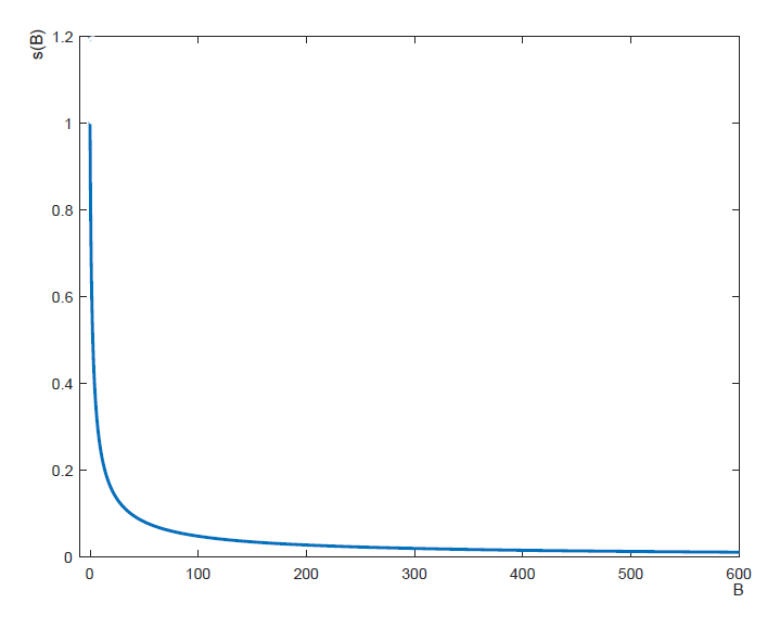
Figure 2: The image of the function $B\mapsto s(B)$

4.1 Upper bound of $\dim_{\mathrm{H}}F(B)$

The upper bound estimation of $\dim_{\mathrm{H}}F(B)$ is by a natural covering. We denote the interval

$$J(d_{1},\cdots,d_{n})=\{x\in(0,1]:d_{k}(x)=d_{k},1\leq k\leq n,d_{n+1}(x)\geq B(n+1)\}.$$

We have that

$$F(B)= \bigcap_{N\geq 1}\bigcup_{n\geq N}\bigcup_{(d_{1},\cdots,d_{n})\in\mathbb{N}^{n}}J(d_{1},\cdots,d_{n}),$$

$$|J(d_{1},\cdots,d_{n})|= \sum_{d_{n+1}\geq B(n+1)}|I_{n+1}(d_{1},\cdots,d_{n},d_{n+1})|\leq\frac{1}{2^{d_{1}+\cdots+d_{n}}\cdot 2^{B(n+1)}}.$$

Therefore, for any $\varepsilon>0$, we have

$$\mathcal{H}^{s(B)+\varepsilon}(F(B)) \leq\liminf_{N\to\infty}\sum_{n\geq N}\sum_{d_{1},\cdots,d_{n}}|J(d_{1},\cdots,d_{n})|^{s(B)+\varepsilon}$$

$$\leq\liminf_{N\to\infty}\sum_{n\geq N}\sum_{d_{1},\cdots,d_{n}}(\frac{1}{2^{d_{1}+\cdots+d_{n}}\cdot 2^{B(n+1)}})^{s(B)+\varepsilon}$$

$$\leq\liminf_{N\to\infty}\sum_{n\geq N}\sum_{d_{1},\cdots,d_{n}}(\frac{1}{2^{d_{1}+\cdots+d_{n}}\cdot 2^{Bn}})^{s(B)}(\frac{1}{2^{d_{1}+\cdots+d_{n}}\cdot 2^{Bn}})^{\varepsilon}$$

$$\leq\liminf_{N\to\infty}\sum_{n\geq N}\sum_{d_{1},\cdots,d_{n}}(\frac{1}{2^{d_{1}+\cdots+d_{n}}\cdot 2^{Bn}})^{s(B)}(\frac{1}{2^{n}\cdot 2^{Bn}})^{\varepsilon}$$

$$=\liminf_{N\to\infty}\sum_{n\geq N}(\frac{1}{2^{n}\cdot 2^{Bn}})^{\varepsilon}=0,$$

where $\mathcal{H}^{s}$ stands for the s-dimensional Hausdorff measure and the penultimate equality is by the equation (4.1). This implies $\dim_{\mathrm{H}}F(B)\leq s(B)+\varepsilon$. Due to the arbitrariness of $\varepsilon$, we conclude that $\dim_{\mathrm{H}}F(B)\leq s(B)$.

4.2 Lower bound of $\dim_{\mathrm{H}}F(B)$

It suffices for proving the case $0<B<\infty$. To establish the lower bound of $\dim_{\mathrm{H}}F(B)$, we will construct a subset $F_{M}(B)\subset F(B)$ and use the Hausdorff dimension of $F_{M}(B)$ to approximate that of $F(B)$.

4.2.1 Construction of subset $F_{M}(B)$ of $F(B)$

Fix a sufficiently small $\epsilon>0$ and $B>0$, we define a sequence $\{n_{k}\}_{k\in\mathbb{N}}$ recursively as follows:

$$n_{1}= \min\{n:\lfloor(1+\epsilon)Bn\rfloor-\lfloor Bn\rfloor>1\},$$

$$n_{1}+ n_{2}+\cdots+n_{k}\leq\frac{1}{k+1}n_{k+1},\qquad\forall k\geq 1.$$ (4.2)

Let $M\in\mathbb{N}$ and $F_{M}(B)$ be a subset of $F(B)$ defined as

$$F_{M}(B)=\{ x\in I:\lfloor Bn_{k}\rfloor+1\leq d_{n_{k}}(x)\leq\lfloor(1+\epsilon)Bn_{k}\rfloor,~{}\text{for all}~{}k\geq 1,$$

$$\text{and}~{}1\leq d_{j}(x)\leq M,~{}\text{for all}~{}j\neq n_{k}\}.$$

Denote by $s_{M}(B)$ the unique real solution of the equation

$$\sum_{k=1}^{M}\Big{(}\frac{1}{2^{B}2^{k}}\Big{)}^{s}=1.$$

Remark 4.1.

By the definition of $s(B)$ and $s_{M}(B)$, we have

$$\lim_{M\to\infty}s_{M}(B)=s(B).$$

Now we provide a symbolic description of the structure of $F_{M}(B)$. Let

$$D_{n}= \{(\sigma_{1},\cdots,\sigma_{n})\in\mathbb{N}^{n}:\lfloor Bn_{k}\rfloor+1\leq\sigma_{n_{k}}\leq\lfloor(1+\epsilon)Bn_{k}\rfloor,$$

$$~{}\text{for all}~{}k\geq 1,1\leq n_{k}\leq n,~{}\text{and}~{}1\leq\sigma_{j}\leq M,~{}\forall j\neq n_{k},1\leq j\leq n\},$$

$$D= \bigcup_{n=1}^{\infty}D_{n}.$$

For any $n\geq 1$ and any $(\sigma_{1},\cdots,\sigma_{n})\in D_{n}$, we call $I_{n}(\sigma_{1},\cdots,\sigma_{n})$ an $n$-th basic interval. Additionally,

$$J(\sigma_{1},\cdots,\sigma_{n})=\bigcup_{\sigma_{n+1}:(\sigma_{1},\cdots,\sigma_{n+1})\in D_{n+1}}I_{n+1}(\sigma_{1},\cdots,\sigma_{n},\sigma_{n+1})$$ (4.3)

is termed an $n$-th fundamental interval. According to (2.5), if $n+1\neq n_{k}$ for any $k\geq 1$, then

$$|J(\sigma_{1},\cdots,\sigma_{n})|=\frac{1}{2^{\sigma_{1}+\cdots+\sigma_{n}}}(1-\frac{1}{2^{M}}),$$ (4.4)

and, if $n+1=n_{k}$ for some $k\geq 1$, then

$$|J(\sigma_{1},\cdots,\sigma_{n})|=\frac{1}{2^{\sigma_{1}+\cdots+\sigma_{n}}}(\frac{1}{2^{\lfloor Bn_{k}\rfloor}}-\frac{1}{2^{\lfloor(1+\epsilon)Bn_{k}\rfloor}}).$$ (4.5)

It is easily seen that

$$F_{M}(B)=\bigcap_{n\geq 1}\bigcup_{(\sigma_{1},\cdots,\sigma_{n})\in D_{n}}J(\sigma_{1},\cdots,\sigma_{n}).$$ (4.6)

4.2.2 A mass distribution on $F_{M}(B)$

In this subsection, we define a probability measure supported on $F_{M}(B)$ and give the estimation of $\mu(J(\sigma_{1},\cdots,\sigma_{n}))$ for each $(\sigma_{1},\cdots,\sigma_{n})\in D_{n}$, by using the length $|J(\sigma_{1},\cdots,\sigma_{n})|$.

Lemma 4.1.

We can define a probability measure $\mu$ supported on $F_{M}(B)$ such that

$$\mu(J(\sigma_{1},\cdots,\sigma_{n}))\leq C|J(\sigma_{1},\cdots,\sigma_{n})|^{(1-\epsilon)s_{M}(B)},$$ (4.7)

where $C$ is a constant dependent of $\epsilon$, $M$ and $B$.

Proof.

Fix $\epsilon>0$, we define a set function $\mu:\{J(\sigma):\sigma\in D\}\to\mathbb{R}^{+}$ as follows. For any $n<n_{1}$ and $(\sigma_{1},\cdots,\sigma_{n})\in D_{n}$, let

$$\mu(J(\sigma_{1},\cdots,\sigma_{n}))=\prod_{i=1}^{n}(\frac{1}{2^{B}2^{\sigma_{i}}})^{s_{M}(B)}.$$

For any $(\sigma_{1},\cdots,\sigma_{n_{1}})\in D_{n_{1}}$, set

$$\mu(J(\sigma_{1},\cdots,\sigma_{n_{1}}))=\frac{1}{\lfloor(1+\epsilon)Bn_{1}\rfloor-\lfloor Bn_{1}\rfloor}\mu(J(\sigma_{1},\cdots,\sigma_{n_{1}-1})).$$

Once $\mu(J(\sigma_{1},\cdots,\sigma_{n_{k}}))$ has been defined for some $k>1$ and any $(\sigma_{1},\cdots,\sigma_{n_{k}})\in D_{n_{k}}$, we define, for any $n_{k}<n<n_{k+1}$ and any $(\sigma_{1},\cdots,\sigma_{n})\in D_{n}$,

$$\mu(J(\sigma_{1},\cdots,\sigma_{n}))=\mu(J(\sigma_{1},\cdots,\sigma_{n_{k}}))\prod_{i=n_{k}+1}^{n}(\frac{1}{2^{B}2^{\sigma_{i}}})^{s_{M}(B)},$$

and

$$\mu(J(\sigma_{1},\cdots,\sigma_{n_{k+1}}))=\frac{1}{\lfloor(1+\epsilon)Bn_{k+1}\rfloor-\lfloor Bn_{k+1}\rfloor}\mu(J(\sigma_{1},\cdots,\sigma_{n_{k+1}-1})),$$

for any $(\sigma_{1},\cdots,\sigma_{n_{k+1}})\in D_{n_{k+1}}$.

It can be verified that for any $n\geq 1$ and $(\sigma_{1},\cdots,\sigma_{n})\in D_{n}$, we have

$$\mu(J(\sigma_{1},\cdots,\sigma_{n}))=\sum_{\sigma_{n+1}:(\sigma_{1},\cdots,\sigma_{n+1})\in D_{n+1}}\mu(J(\sigma_{1},\cdots,\sigma_{n},\sigma_{n+1})),$$

and

$$\sum_{\sigma_{1}\in D_{1}}\mu(J(\sigma_{1}))=1.$$

Thus $\mu$ can be extended to a probability measure supported on $F_{M}(B)$ due to Kolmogorov’s extension theorem. We denote the measure still by $\mu$. By the definition of $\mu$, for any $k\geq 1$, $n_{k}\leq n<n_{k+1}$ and any $(\sigma_{1},\cdots,\sigma_{n})\in D_{n}$, we have

$$\mu(J(\sigma_{1},\cdots,\sigma_{n}))=\prod_{j=1}^{k}\frac{1}{\lfloor(1+\epsilon)Bn_{j}\rfloor-\lfloor Bn_{j}\rfloor}\prod_{i\in\Delta_{n}}(\frac{1}{2^{B}2^{\sigma_{i}}})^{s_{M}(B)},$$ (4.8)

where the notation $\Delta_{n}=\{1\leq i\leq n:i\neq n_{j}~{}\text{for any}~{}j\}$.

Case 1. $n=n_{k}$ for some $k\geq 1$. In this case, by (4.4) and (4.8), we have

$$\mu(J(\sigma_{1},\cdots,\sigma_{n})) =\prod_{j=1}^{k}\frac{1}{\lfloor(1+\epsilon)Bn_{j}\rfloor-\lfloor Bn_{j}\rfloor}\prod_{i\in\Delta_{n_{k}}}(\frac{1}{2^{B}2^{\sigma_{i}}})^{s_{M}(B)}$$

$$=\prod_{j=1}^{k}\frac{1}{\lfloor(1+\epsilon)Bn_{j}\rfloor-\lfloor Bn_{j}\rfloor}2^{-(\sum_{i\in\Delta_{n_{k}}}\sigma_{i}+B(n-k))s_{M}(B)},$$

and

$$|J(\sigma_{1},\cdots,\sigma_{n})|=2^{-\sum_{i=1}^{n}\sigma_{i}}(1-\frac{1}{2^{M}}).$$

Note that

$$B\leq\lim_{k\to\infty}\frac{\sum_{j=1}^{k}\sigma_{n_{j}}}{n_{k}}\leq B(1+\epsilon)\qquad\text{and}\qquad\lim_{k\to\infty}\frac{\sum_{i=1}^{n}\sigma_{i}}{n_{k}}\geq 1+B.$$ (4.9)

For fixed $\epsilon>0$, there exists $k_{0}$ dependent of $\epsilon$, $M$ and $B$, such that for all $k>k_{0}$, we have

$$\sum_{i=1}^{n}\sigma_{i}(1-\epsilon)s_{M}(B)\leq\sum_{i\in\Delta_{n}}\sigma_{i}s_{M}(B)+Bs_{M}(B)(n-k).$$

Hence, there exists $c_{0}>0$ such that

$$\mu(J(\sigma_{1},\cdots,\sigma_{n}))\leq c_{0}|J(\sigma_{1},\cdots,\sigma_{n})|^{(1-\epsilon)s_{M}(B)}.$$ (4.10)

Case 2. $n+1=n_{k}$ for some $k\geq 1$. In this case, by (4.5) and (4.8), we have

$$\mu(J(\sigma_{1},\cdots,\sigma_{n})) =\prod_{j=1}^{k-1}\frac{1}{\lfloor(1+\epsilon)Bn_{j}\rfloor-\lfloor Bn_{j}\rfloor}2^{-(\sum_{i\in\Delta_{n}}\sigma_{i}+B(n-k+1))s_{M}(B)},$$

$$|J(\sigma_{1},\cdots,\sigma_{n})| =2^{-\sum_{i=1}^{n}\sigma_{i}}(\frac{1}{2^{\lfloor Bn_{k}\rfloor}}-\frac{1}{2^{\lfloor(1+\epsilon)Bn_{k}\rfloor}}).$$

Thus, there exists $c_{1}>0$ such that

$$c_{1}2^{-\sum_{i=1}^{n}\sigma_{i}}\frac{1}{2^{Bn_{k}}}\leq|J(\sigma_{1},\cdots,\sigma_{n})|\leq 2^{-\sum_{i=1}^{n}\sigma_{i}}\frac{1}{2^{Bn_{k}}}.$$

By choosing a sufficient large $k_{0}$, we have

$$\sum_{i\in\Delta_{n}}\sigma_{i}s_{M}(B)+Bs_{M}(B)(n-k+1)\geq\sum_{i=1}^{n}\sigma_{i}(1-\epsilon)s_{M}(B)+Bn_{k}(1-\epsilon)s_{M}(B),\qquad\forall k\geq k_{0}.$$

Then, there exists $c_{2}>0$ such that

$$\mu(J(\sigma_{1},\cdots,\sigma_{n}))\leq c_{2}|J(\sigma_{1},\cdots,\sigma_{n})|^{(1-\epsilon)s_{M}(B)}.$$ (4.11)

Case 3. $n_{k-1}<n<n_{k}-1$ for some $k\geq 1$, by (4.4) and (4.8), we have

$$\mu(J(\sigma_{1},\cdots,\sigma_{n})) =\prod_{j=1}^{k-1}\frac{1}{\lfloor(1+\epsilon)Bn_{j}\rfloor-\lfloor Bn_{j}\rfloor}2^{-(\sum_{i\in\Delta_{n}}\sigma_{i}+B(n-k+1))s_{M}(B)},$$

$$|J(\sigma_{1},\cdots,\sigma_{n})| =2^{-\sum_{i=1}^{n}\sigma_{i}}(1-\frac{1}{2^{M}}).$$

By choosing the $k_{0}$ again, we have

$$\sum_{i=1}^{n}\sigma_{i}(1-\epsilon)s_{M}(B)\leq\sum_{i\in\Delta_{n}}\sigma_{i}s_{M}(B)+Bs_{M}(B)(n-k+1),\qquad\forall k\geq k_{0}.$$

Hence, there exists $c_{3}>0$ such that

$$\mu(J(\sigma_{1},\cdots,\sigma_{n}))\leq c_{3}|J(\sigma_{1},\cdots,\sigma_{n})|^{(1-\epsilon)s_{M}(B)}.$$ (4.12)

By taking $C=\max\{c_{0},c_{2},c_{3}\}$, we can deduce from (4.10), (4.11) and (4.12) that

$$\mu(J(\sigma_{1},\cdots,\sigma_{n}))\leq C|J(\sigma_{1},\cdots,\sigma_{n})|^{(1-\epsilon)s_{M}(B)}.$$

∎

4.2.3 Estimation of gaps between fundamental intervals

In this subsection, we focus on estimating the gaps between disjoint fundamental intervals, as defined in (4.3), of the same order. For each $(\sigma_{1},\cdots,\sigma_{n})\in D_{n}$, , we denote the distance between $J(\sigma_{1},\cdots,\sigma_{n})$ and the nearest fundamental interval of the same order on its right (left, respectively) as $g^{r}(\sigma_{1},\cdots,\sigma_{n})$ ($g^{l}(\sigma_{1},\cdots,\sigma_{n})$, respectively). We define the gap as

$$g(\sigma_{1},\cdots,\sigma_{n}):=\min\{g^{r}(\sigma_{1},\cdots,\sigma_{n}),g^{l}(\sigma_{1},\cdots,\sigma_{n})\}.$$

Case 1: $n+1\neq n_{k}$ for any $k\geq 1$. In this case, the left and right endpoint of $J(\sigma_{1},\cdots,\sigma_{n})$ are

$$\sum_{i=1}^{n}\frac{1}{2^{\sigma_{1}+\cdots+\sigma_{i}}}+\frac{1}{2^{\sigma_{1}+\cdots+\sigma_{n}+M}}\qquad\text{and}\qquad\sum_{i=1}^{n}\frac{1}{2^{\sigma_{1}+\cdots+\sigma_{i}}}+\frac{1}{2^{\sigma_{1}+\cdots+\sigma_{n}}}.$$

If there exists $1\leq i_{0}\leq n$ such that $(\sigma_{1},\cdots,\sigma_{i_{0}}+1,\cdots,\sigma_{n})\in D_{n}$ and $J(\sigma_{1},\cdots,\sigma_{i_{0}}+1,\cdots,\sigma_{n})$ is the nearest $n$-th fundamental interval lying on the left of $J(\sigma_{1},\cdots,\sigma_{n})$, then $g^{l}(\sigma_{1},\cdots,\sigma_{n})$ is precisely the distance between the left endpoint of $J(\sigma_{1},\cdots,\sigma_{n})$ and the right endpoint of $J(\sigma_{1},\cdots,\sigma_{i_{0}}+1,\cdots,\sigma_{n})$. Thus

$$g^{l}(\sigma_{1},\cdots,\sigma_{n}) =\sum_{i=1}^{n}\frac{1}{2^{\sigma_{1}+\cdots+\sigma_{i}}}+\frac{1}{2^{\sigma_{1}+\cdots+\sigma_{n}+M}}-\Big{(}\sum_{i=1}^{i_{0}-1}\frac{1}{2^{\sigma_{1}+\cdots+\sigma_{i}}}+\sum_{i=i_{0}}^{n}\frac{1}{2^{\sigma_{1}+\cdots+\sigma_{i}+1}}+\frac{1}{2^{\sigma_{1}+\cdots+\sigma_{n}+1}}\Big{)}$$

$$=\sum_{i=i_{0}}^{n-1}\frac{1}{2^{\sigma_{1}+\cdots+\sigma_{i}+1}}+\frac{1}{2^{\sigma_{1}+\cdots+\sigma_{n}+M}}\geq\frac{1}{2^{\sigma_{1}+\cdots+\sigma_{n}+M}}.$$

If there exists $1\leq i_{1}\leq n$ such that $(\sigma_{1},\cdots,\sigma_{i_{1}}-1,\cdots,\sigma_{n})\in D_{n}$ and $J(\sigma_{1},\cdots,\sigma_{i_{1}}-1,\cdots,\sigma_{n})$ is the nearest $n$-th fundamental interval on the right of $J(\sigma_{1},\cdots,\sigma_{n})$, then $g^{r}(\sigma_{1},\cdots,\sigma_{n})$ is just the distance between the right endpoint of $J(\sigma_{1},\cdots,\sigma_{n})$ and the left endpoint of $J(\sigma_{1},\cdots,\sigma_{i_{1}}-1,\cdots,\sigma_{n})$. Thus

$$g^{r}(\sigma_{1},\cdots,\sigma_{n}) =\sum_{i=1}^{i_{1}-1}\frac{1}{2^{\sigma_{1}+\cdots+\sigma_{i}}}+\sum_{i=i_{1}}^{n}\frac{1}{2^{\sigma_{1}+\cdots+\sigma_{i}-1}}+\frac{1}{2^{\sigma_{1}+\cdots+\sigma_{n}+M-1}}-\Big{(}\sum_{i=1}^{n}\frac{1}{2^{\sigma_{1}+\cdots+\sigma_{i}}}+\frac{1}{2^{\sigma_{1}+\cdots+\sigma_{n}}}\Big{)}$$

$$=\sum_{i=i_{1}}^{n-1}\frac{1}{2^{\sigma_{1}+\cdots+\sigma_{i}}}+\frac{1}{2^{\sigma_{1}+\cdots+\sigma_{n}+M-1}}\geq\frac{1}{2^{\sigma_{1}+\cdots+\sigma_{n}+M-1}}.$$

Hence

$$g(\sigma_{1},\cdots,\sigma_{n})\geq\frac{1}{2^{\sigma_{1}+\cdots+\sigma_{n}+M}}.$$ (4.13)

Case 2: $n+1=n_{k}$ for some $k\geq 1$.

In this case, $g^{l}(\sigma_{1},\cdots,\sigma_{n})$ is larger than the distance between the left endpoint of $I(\sigma_{1},\cdots,\sigma_{n})$ and the left endpoint of $J(\sigma_{1},\cdots,\sigma_{n})$, $g^{r}(\sigma_{1},\cdots,\sigma_{n})$ is larger than the distance between the right endpoint of $I(\sigma_{1},\cdots,\sigma_{n})$ and the right endpoint of $J(\sigma_{1},\cdots,\sigma_{n})$. Thus

$$g^{l}(\sigma_{1},\cdots,\sigma_{n}) \geq\sum_{i=1}^{n}\frac{1}{2^{\sigma_{1}+\cdots+\sigma_{i}}}+\frac{1}{2^{\sigma_{1}+\cdots+\sigma_{n}+\lfloor(1+\epsilon)Bn_{k}\rfloor}}-\sum_{i=1}^{n}\frac{1}{2^{\sigma_{1}+\cdots+\sigma_{i}}}$$

$$=\frac{1}{2^{\sigma_{1}+\cdots+\sigma_{n}}}\cdot\frac{1}{2^{\lfloor(1+\epsilon)Bn_{k}\rfloor}},$$

$$g^{r}(\sigma_{1},\cdots,\sigma_{n}) \geq\sum_{i=1}^{n-1}\frac{1}{2^{\sigma_{1}+\cdots+\sigma_{i}}}+\frac{1}{2^{\sigma_{1}+\cdots+\sigma_{n}-1}}-\Big{(}\sum_{i=1}^{n}\frac{1}{2^{\sigma_{1}+\cdots+\sigma_{i}}}+\frac{1}{2^{\sigma_{1}+\cdots+\sigma_{n}+\lfloor Bn_{k}\rfloor}}\Big{)}$$

$$=\frac{1}{2^{\sigma_{1}+\cdots+\sigma_{n}}}(1-\frac{1}{2^{\lfloor Bn_{k}\rfloor}}).$$

Hence

$$g(\sigma_{1},\cdots,\sigma_{n})\geq\frac{1}{2^{\sigma_{1}+\cdots+\sigma_{n}}}\cdot\frac{1}{2^{\lfloor(1+\epsilon)Bn_{k}\rfloor}}.$$ (4.14)

If $n+1\neq n_{k}$ for any $k\geq 1$, by (4.4) and (4.13), we have

$$g(\sigma_{1},\cdots,\sigma_{n})\geq\frac{1}{2^{M}-1}|J(\sigma_{1},\cdots,\sigma_{n})|.$$

If $n+1=n_{k}$ for some $k\geq 1$, by (4.5) and (4.14), we have

$$g(\sigma_{1},\cdots,\sigma_{n})\geq\frac{1}{2^{\lfloor\epsilon Bn_{k}\rfloor+1}-1}|J(\sigma_{1},\cdots,\sigma_{n})|.$$

4.2.4 Lower bound of $\dim_{\mathrm{H}}F_{M}(B)$

In this subsection, we apply the mass distribution principle [1, Proposition 4.2] to obtain the lower bound of $\dim_{\mathrm{H}}F_{M}(B)$.

Lemma 4.2.

Let $F_{M}(B)$ be defined as in (4.6), then

$$\dim_{\mathrm{H}}F_{M}(B)\geq(1-2\epsilon)s_{M}(B).$$

Proof.

For $n\geq 1$ and $(\sigma_{1},\cdots,\sigma_{n})\in D_{n}$,

1. if $n+1\neq n_{k}$ for any $k\geq 1$, set

   $$g_{1}(\sigma_{1},\cdots,\sigma_{n}):=\frac{1}{2^{\sigma_{1}+\cdots+\sigma_{n}}2^{M}}\geq\frac{1}{2^{M}-1}|J(\sigma_{1},\cdots,\sigma_{n})|,$$ (4.15)

2. if $n+1=n_{k}$ for some $k\geq 1$, set

   $$g_{1}(\sigma_{1},\cdots,\sigma_{n}):=\frac{1}{2^{\sigma_{1}+\cdots+\sigma_{n}}2^{\lfloor(1+\epsilon)Bn_{k}\rfloor}}\geq\frac{1}{2^{\lfloor\epsilon Bn_{k}\rfloor+1}-1}|J(\sigma_{1},\cdots,\sigma_{n})|.$$ (4.16)

Define $r_{0}=\min\limits_{1\leq j\leq n_{k_{0}}}\min\limits_{(\sigma_{1},\cdots,\sigma_{j})\in D_{j}}g_{1}(\sigma_{1},\cdots,\sigma_{j})$. For a fixed $x\in F_{M}(B)$ and $0<r<r_{0}$ and set $\sigma_{i}=d_{i}(x)$. Then $x\in J(\sigma_{1},\cdots,\sigma_{k})$ for all $k\geq 1$ and there exists some $n\geq n_{k_{0}}$, such that

$$g_{1}(\sigma_{1},\cdots,\sigma_{n},\sigma_{n+1})\leq r<g_{1}(\sigma_{1},\cdots,\sigma_{n}).$$

By the definition of $g_{1}(\sigma_{1},\cdots,\sigma_{n})$, the ball $B(x,r)$ can intersect only one fundamental interval of order $n$, which is precisely $J(\sigma_{1},\cdots,\sigma_{n})$.

Case 1: $n+1=n_{k}$ for some $k\geq k_{0}$.

1. $r\leq\frac{1}{2}|I(\sigma_{1},\cdots.\sigma_{n_{k}})|$. In this case, the ball $B(x,r)$ can intersect at most three basic intervals of order $n_{k}$, which are $I(\sigma_{1},\cdots.\sigma_{n_{k}}-1),I(\sigma_{1},\cdots.\sigma_{n_{k}}),I(\sigma_{1},\cdots.\sigma_{n_{k}}+1)$ (if exist). Hence, we have

   $$\mu(B(x,r))\leq 3\mu(J(\sigma_{1},\cdots.\sigma_{n_{k}})).$$

   By Lemma 4.1 and (4.15), we have

   $$\mu(B(x,r)) \leq 3C|J(\sigma_{1},\cdots.\sigma_{n_{k}})|^{(1-\epsilon)s_{M}(B)}\leq 3(2^{M}-1)Cg_{1}(\sigma_{1},\cdots.\sigma_{n_{k}})^{(1-\epsilon)s_{M}(B)}$$ (4.17)

   $$\leq 3(2^{M}-1)Cr^{(1-\epsilon)s_{M}(B)}.$$

2. $r\geq\frac{1}{2}|I(\sigma_{1},\cdots.\sigma_{n_{k}})|$. In this case, since

   $$|I(\sigma_{1},\cdots.\sigma_{n_{k}})|=\frac{1}{2^{\sigma_{1}+\cdots+\sigma_{n_{k}-1}}}\cdot\frac{1}{2^{\sigma_{n_{k}}}}\geq\frac{1}{2^{\sigma_{1}+\cdots+\sigma_{n_{k}-1}}}\cdot\frac{1}{2^{\lfloor(1+\epsilon)Bn_{k}\rfloor}},$$

   there are at most $2r2^{\sigma_{1}+\cdots+\sigma_{n_{k}-1}}2^{\lfloor(1+\epsilon)Bn_{k}\rfloor}$ fundamental intervals of order $n_{k}$ contained in $J(\sigma_{1},\cdots.\sigma_{n_{k}-1})$ and intersecting the ball $B(x,r)$. Then, by (4.5) and Lemma 4.1, we have

   $$\mu(B(x,r))\leq\mu(J(\sigma_{1},\cdots.\sigma_{n_{k}-1}))\min\Big{\{}1,2r2^{\sigma_{1}+\cdots+\sigma_{n_{k}-1}}2^{\lfloor(1+\epsilon)Bn_{k}\rfloor}\frac{1}{\lfloor(1+\epsilon)Bn_{k}\rfloor-\lfloor Bn_{k}\rfloor}\Big{\}}$$

   $$\leq C|J(\sigma_{1},\cdots.\sigma_{n_{k}-1})|^{(1-\epsilon)s_{M}(B)}\min\Big{\{}1,2r2^{\sigma_{1}+\cdots+\sigma_{n_{k}-1}}2^{\lfloor(1+\epsilon)Bn_{k}\rfloor}\frac{1}{\lfloor(1+\epsilon)Bn_{k}\rfloor-\lfloor Bn_{k}\rfloor}\Big{\}}$$

   $$\leq C|J(\sigma_{1},\cdots.\sigma_{n_{k}-1})|^{(1-\epsilon)s_{M}(B)}\Big{(}2r2^{\sigma_{1}+\cdots+\sigma_{n_{k}-1}}2^{\lfloor(1+\epsilon)Bn_{k}\rfloor}\frac{1}{\lfloor(1+\epsilon)Bn_{k}\rfloor-\lfloor Bn_{k}\rfloor}\Big{)}^{(1-2\epsilon)s_{M}(B)}$$

   $$\leq C\Big{(}\frac{2r}{\lfloor(1+\epsilon)Bn_{k}\rfloor-\lfloor Bn_{k}\rfloor}\Big{)}^{(1-2\epsilon)s_{M}(B)}2^{-\sum_{i=1}^{n_{k}-1}\epsilon s_{M}(B)\sigma_{i}}.$$

   Thus, there exists $c_{4}$ such that

   $$\mu(B(x,r))\leq c_{4}r^{(1-2\epsilon)s_{M}(B)}.$$ (4.18)

Case 2: $n+1\neq n_{k}$ and $n+2\neq n_{k}$ for any $k\geq k_{0}$.

For any $1\leq\xi<\zeta\leq M$, by the definition of $\mu$, we have

$$\frac{\mu(J(\sigma_{1},\cdots,\sigma_{n},\xi))}{\mu(J(\sigma_{1},\cdots,\sigma_{n},\zeta))}\leq 2^{M-1}.$$

Then, by Lemma 4.1 and (4.15), we have

$$\mu(B(x,r)) \leq M2^{M-1}\mu(J(\sigma_{1},\cdots,\sigma_{n+1}))$$

$$\leq CM2^{M-1}|J(\sigma_{1},\cdots,\sigma_{n+1})|^{(1-\epsilon)s_{M}(B)}$$

$$\leq CM2^{2M-1}g_{1}(\sigma_{1},\cdots,\sigma_{n+1})^{(1-\epsilon)s_{M}(B)}$$

$$\leq CM2^{2M-1}r^{(1-\epsilon)s_{M}(B)}.$$ (4.19)

Case 3: $n+2=n_{k}$ for any $k\geq k_{0}$.

Similar to Case II, we deduce from Lemma 4.1 and (4.16) that

$$\mu(B(x,r)) \leq M2^{M-1}\mu(J(\sigma_{1},\cdots,\sigma_{n+1}))$$

$$\leq CM2^{M-1}|J(\sigma_{1},\cdots,\sigma_{n+1})|^{(1-\epsilon)s_{M}(B)}$$

$$\leq CM2^{M-1}(2^{\lfloor\epsilon Bn_{k}\rfloor+1}-1)^{(1-\epsilon)s_{M}(B)}g_{1}(\sigma_{1},\cdots,\sigma_{n+1})^{(1-\epsilon)s_{M}(B)}$$

$$\leq CM2^{M-1}g_{1}(\sigma_{1},\cdots,\sigma_{n+1})^{(1-\epsilon)^{2}s_{M}(B)}$$

$$\leq CM2^{M-1}r^{(1-\epsilon)^{2}s_{M}(B)}.$$ (4.20)

As a consequence of mass distribution principle [1, Proposition 4.2] and (4.17) – (4.2.4),

$$\dim_{\mathrm{H}}F_{M}(B)\geq(1-2\epsilon)s_{M}(B).$$

∎

Since $F_{M}(B)\subset F(B)$, by taking $\epsilon\to 0$, it holds

$$\dim_{\mathrm{H}}F(B)\geq\dim_{\mathrm{H}}F_{M}(B)\geq s_{M}(B).$$

As $M\to\infty$, by Remark 4.1, we obtain

$$\dim_{\mathrm{H}}F(B)\geq s(B).$$

Corollary 4.1.

For any infinite set $\mathcal{A}\subset\mathbb{N}$,

$$\dim_{\mathrm{H}}\{x\in I:d_{n}(x)\geq Bn~{}~{}\text{i.m.}~{}n\in\mathcal{A}\}=s(B).$$

Proof.

It follows by choosing the integer sequence $\{n_{k}\}_{k\geq 1}$ satisfying (4.2.1) and $n_{k}\in\mathcal{A}$ for all $k\geq 2$ in the proof of Theorem 1.2. ∎

5 Proof of Theorem 1.3

Proof.

1. If $B=0$, then for any $\varepsilon>0$, $\phi(n)\leq\varepsilon n$ holds for infinitely many $n$’s. Let

   $$\mathcal{A}=\{n:\phi(n)\leq\varepsilon n\}.$$

   Then

   $$\{x\in I:d_{n}(x)\geq\varepsilon n,~{}~{}\text{i.m.}~{}n\in\mathcal{A}\}\subset F(\phi).$$

   By the continuous of $s(\cdot)$ and Corollary 4.1, we have

   $$\dim_{\mathrm{H}}F(\phi)\geq\sup_{\varepsilon>0}s(\varepsilon)=1,$$

   thus $\dim_{\mathrm{H}}F(\phi)=1$.

2. If $0<B<\infty$, then for any $\varepsilon>0$, $\phi(n)\leq(B+\varepsilon)n$ holds for infinitely many $n$’s. On the other hand, there exists $N\in\mathbb{N}$ such that for all $n\geq N$, we have $(B-\varepsilon)n\leq\phi(n)$. Let

   $$\mathcal{A}=\{n:\phi(n)\leq(B+\varepsilon)n\}.$$

   Then

   $$\{x\in I:d_{n}(x)\geq(B+\varepsilon)n,~{}~{}\text{i.m.}~{}n\in\mathcal{A}\}\subset F(\phi)\subset\{x\in I:d_{n}(x)\geq(B-\varepsilon)n,~{}~{}\text{i.m.}~{}n\}.$$

   By the continuous of $s(\cdot)$ and Corollary 4.1 again, we have

   $$s(B)=\lim_{\varepsilon\to 0}s(B+\varepsilon)\leq\dim_{\mathrm{H}}F(\phi)\leq\lim_{\varepsilon\to 0}s(B-\varepsilon)=s(B).$$

3. If $B=\infty$, then for any $B_{1}\geq 0$, $\phi(n)\geq B_{1}n$ holds ultimately. Then

   $$F(\phi)\subset\{x\in I:d_{n}(x)\geq B_{1}n,~{}~{}\text{i.m.}~{}n\}.$$

   Thus

   $$\dim_{\mathrm{H}}F(\phi)\leq s(B_{1}).$$

   Letting $B_{1}\to\infty$ gives

   $$\dim_{\mathrm{H}}E(\phi)=0.$$

∎

References

- [1] Falconer, Kenneth. Fractal geometry: Mathematical Foundations and Applications. John Wiley & Sons, 2004.
- [2] Neunhäuserer, Jörg. On the Hausdorff dimension of fractals given by certain expansions of real numbers. Archiv der Mathematik, 97(5):459–466,2011.
- [3] Neunhäuserer, Jörg. On the dimension of certain sets araising in the base two expansion. arXiv:2201.09641.
- [4] Shen, Luming. Hausdorff dimension of the set concerning with Borel-Bernstein theory in Lüroth expansions. Journal of the Korean Mathematical Society, 54(4):1301–1316,2017.
- [5] Wang, Bao-Wei and Wu, Jun. Hausdorff dimension of certain sets arising in continued fraction expansions. Advances in Mathematics, 218(5):1319–1339,2008.