A Crosstalk-Aware Timing Prediction Method in Routing

Abstract.

With shrinking interconnect spacing in advanced technology nodes, existing timing predictions become less precise due to the challenging quantification of crosstalk-induced delay. During the routing, the crosstalk effect is typically modeled by predicting coupling capacitance with congestion information. However, the timing estimation tends to be overly pessimistic, as the crosstalk-induced delay depends not only on the coupling capacitance but also on the signal arrival time. This work presents a crosstalk-aware timing estimation method using a two-step machine learning approach. Interconnects that are physically adjacent and overlap in signal timing windows are filtered first. Crosstalk delay is predicted by integrating physical topology and timing features without relying on post-routing results and the parasitic extraction. Experimental results show a match rate of over 99% for identifying crosstalk nets compared to the commercial tool on the OpenCores benchmarks, with prediction results being more accurate than those of other state-of-the-art methods.

1. Introduction

For low-power, high-performance integrated designs, interconnect delay becomes a bottleneck affecting chip performance in advanced technology nodes (IE, ). Net delay prediction is normally over pessimistic in routing since accurate net information can only be obtained after routing and parasitic extraction (d23, ). The pessimistic prediction leads to repetitive routing iterations, which is unacceptable and time-consuming. Besides, cross-coupling between physically adjacent nets gets more complex with higher cell density (XT, ) and causes undesirable crosstalk noise (C20, ). Crosstalk effect depends on the switching state, the arrival time on the net (victim) being analyzed, and its coupled nets (aggressors) (C20, ). The transition slowdown or speedup on the victim net is represented as delta delay and the timing-window overlap is quantified by the skew of input signal arrival time. Figure 1 shows an example of crosstalk in which the victim net $B$ is coupled with two aggressors. The transition on aggressor net $A$ will result in a delta delay (purple font) on victim net $B$ with a timing window overlap. Paths containing $B$ may suffer a setup or hold violation due to these switches in transition. On the contrary, the transition on aggressor net $C$ has no effect on net $B$ without a timing window overlap.

The complexity of delay computation makes crosstalk analysis challenging (XT, ) (SI, ). Dynamic SPICE simulations are the most accurate way, but even a few nets take a long time. Instead, designers rely on crosstalk-aware static timing analysis (STA) tools to capture the effect, such as PrimeTime-SI (PT, ). Based on timing window analysis, delta delay is reasonably considered if the signal timing window of the aggressor net overlaps with that of the victim net. However, the timing-window analysis in those tools requires a post-routing netlist and parasitic information, which is unrealistic during routing iteration optimization.

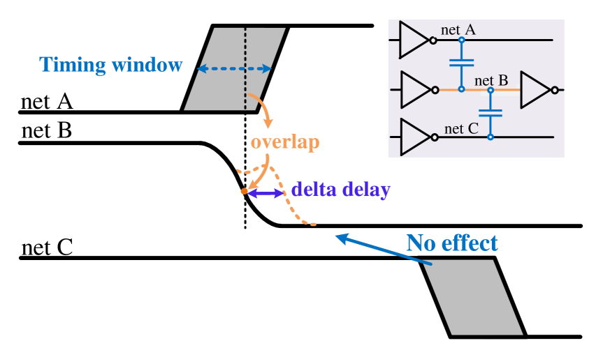
Figure 1. Timing window overlap analysis between adjacent nets and a corresponding delta delay.

Existing crosstalk-aware prediction methods are dedicated to predicting the coupling capacitance using net topology information (22C, )(Lin, ). The crosstalk-induced delay is then considered by estimating the wire density or the coupling capacitance (C20, )(SI, ). This intuitive characterization hinders prediction precision, which pessimistically considers all aggressors who may have non-overlapping timing window as true aggressors. Consequently, designers must add timing margins to account for timing sign-off, causing additional iteration cycles or even suboptimal chip performance.

In this work, a two-step crosstalk-aware timing estimation method is proposed during routing. As depicted in Figure 2, timing-window-related features (purple region) are introduced instead of directly predicting crosstalk by wire density. This makes delay estimation more likely to be post-routing timing results. Physical-related features and timing-related features are extracted for crosstalk net classification and delay prediction. This work can be integrated into traditional routing tools to accelerate timing closure. Our contributions are summarized as follows:

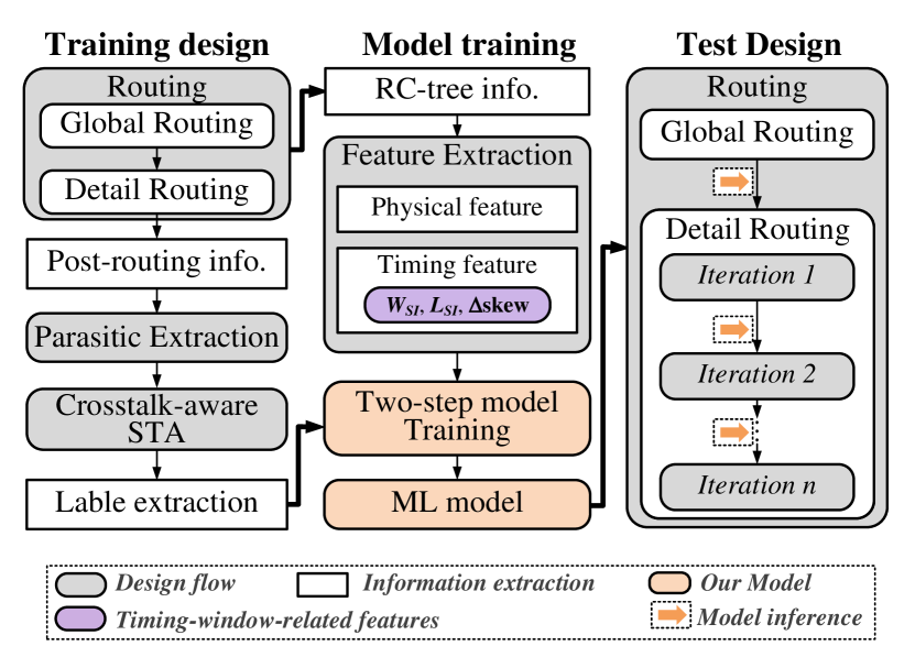
Figure 2. Flowchart of our framework.

• We introduce a novel crosstalk-aware delay prediction method. Relative arrival time between aggressors and victims are extracted, and their effect is quantified for precise crosstalk-induced delay estimation. Interconnects that are physically adjacent but have no overlap in timing windows will be filtered, avoiding prediction complexity and pessimism.

• By integrating physical-related and timing-related features, a two-step machine-learning-based model is proposed to capture crosstalk-induced delay without post-routing netlists and parasitic information. With its flexibility to be integrated into existing routing optimization tools, it shows great potential for application.

The rest of this paper is organized as follows: Section 2 provides a brief overview of prior works. Section 3 details the timing-window-based crosstalk model. Section 4 presents the machine-learning-based model. Section 5 discusses the experimental results. Section 6 concludes the paper.

2. Preliminary

2.1. Machine-Learning-Based Timing Estimation

Recent research endeavors resort to machine learning for timing prediction with high precision (C20, )(22C, )(ml1, ). Barboza et al. (ml1, ) first attempts to predict wire delay and slew during routing with features like pin-to-pin distance and input slew. Hsien-Han Cheng et al. (tree, ) further proposes a loop-breaking algorithm to transform non-tree RC-networks into tree structures using machine learning. A graph neural network model is proposed by Guo et al. (Lin, ) directly predicts total negative slacks and worst negative slacks, losing accuracy in predicting detailed delays. In addition, the crosstalk-induced delay along a timing path can reach 300ps (IE, ), comparable to modern high-performance processor clock periods. Those prediction methods take the routing delay as input, ignoring crosstalk effects (Lin, )(ml1, )(tree, ). The timing prediction results based on those models add an over-pessimistic timing margin to satisfy the performance specification under the crosstalk effect. The machine-learning-based estimation takes crosstalk-induced delay into account but it requires a sign-off timer and only is applied to post-routing designs (SI, ). Liang et al. (C20, ) proposes a graph-based crosstalk prediction method, leveraging neighboring net information. However, crosstalk delay depends not only on the coupling capacitance but also on the signal arrival time.

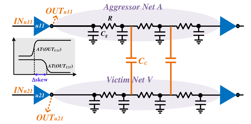
Figure 3. Equivalent circuit for the configuration of two parallel nets.

2.2. Crosstalk Estimation

Crosstalk is the undesirable electrical interaction between two or more physically adjacent nets. In order to analyze the delta delay of the victim due to aggressor activity, the experiment configurations are depicted in Figure 3. The inverter $U_{11}$ drives a long interconnect which is a potential victim net. Aggressor $A$ and victim $V$ run parallel to one another. The capacitive cross-coupling between two interconnects is captured by the coupling capacitance $C_{c}$. The self-capacitance and resistance of the victim net are denoted by $C_{g}$ and $R$, respectively. Interconnect delay is strongly affected by the overlap between timing windows. The overlap between victim and aggressor nets is measured by the skew of the input signal arrival time in (1). If the aggressor overlaps with the victim’s timing window, delta delay is considered.

(1) $$\vspace{0.1cm}\Delta{skew}=AT(OUT_{u11})-AT(OUT_{u21})$$

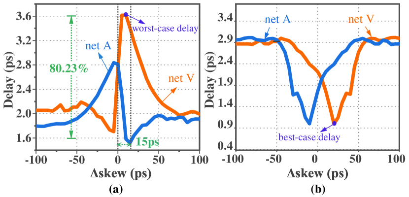
Figure 4. The crosstalk delay induced by input signal with (a) the opposite transitions (b) the consistent transitions, based on HSPICE simulation.

To reveal the correlation, signal transitions are firstly created at the inputs of driver cells, namely $IN_{U11}$ and $IN_{U21}$. The interconnect delay $D_{netA}$ and $D_{netV}$ changes accordingly. The arrival time of the input transition at $IN_{U11}$ is set to 100ps, while the arrival time of the transition at $IN_{U21}$ is swept from 0ps to +200ps. Thus, the input skew between $IN_{U11}$ and $IN_{U21}$ changes accordingly. Figure 4 (a) shows the relation between $\Delta{skew}$ and interconnect delay of net $V$ and net $A$ under opposite input transitions. Delta delay can be highly sensitive to input skew. The worst-case delay has dramatically changed, particularly when the arrival timing window completely overlaps ($\Delta{skew}\to{0}$). For example, a 15ps input skew change can result in 80.23% of the delay change for net $A$. Contrarily, Figure 4 (b) shows the relation between $\Delta{skew}$ and interconnect delay $D_{netA}$ and $D_{netV}$ when signal transitions are generated in the same direction. It can be seen that coupling effects speed up the victim transition and reduce the interconnect delay of the victim net, which corresponds to the best-case delay.

This article mainly focuses on the case where the signal transitions are opposite, since the critical path delay is mainly determined by the worst-case delay. The experiment proves that the crosstalk effect is highly relative to the $\Delta{skew}$.

3. Crosstalk-Aware Timing Prediction

3.1. Timing-Window-Related Feature Selection

Considering the impact of the driver cell on the interconnect segments, the cell delay $D_{driver}$ and the input transition time $S_{in}$ are selected. Therefore, the segment delay without coupling is expressed in (2).

(2) $$\tau_{noSI}=f(D_{driver},S_{in},L)$$

Additionally, Figure 5 gives an example of two interconnects consisting of several segments for adjacent two layers, $M_{3}$ and $M_{4}$. $W_{SI}$ is the width between two crosstalk segments. $L_{SI}$ is the length of coupling segments. $\Delta{skew}$ is the arrival time offset. Hence, quantified by $\Delta{skew}$, $W_{SI}$ and $L_{SI}$, delta delay is modeled as (3) considers the timing window discussed in Section 2.2. It is worth noting that $\Delta{skew}$, $W_{SI}$, and $L_{SI}$ are taken as the timing-window-related features in the following section.

(3) $$\tau_{SI}=f(W_{SI},L_{SI},\Delta{skew})$$

The final delay of a single wire segment is further modeled as (4). The total interconnect delay $D_{net}$ with $N$ segments is given by (5).

(4) $$\tau=\tau_{noSI}+\tau_{SI}$$

(5) $$D_{net}=\sum\nolimits_{i=0}^{N}{\tau(s_{i})}=\sum\nolimits_{i=0}^{N}{\tau_{noSI}(s_{i})}+\underbrace{\sum\nolimits_{i=0}^{M}{\tau_{SI}(s_{i})}}_{delta\ delay}$$

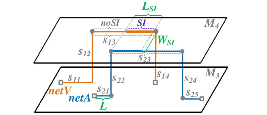
Figure 5. Physically adjacent nets from different layers.

For example, it is observed that crosstalk occurs between segments $s_{13}$ and $s_{23}$ with signal transitions in opposite directions and results in delta delay. We estimate the no-crosstalk delay as $\tau_{noSI}$($s_{13}$) based on (2) and the delta delay of $s_{13}$ as $\tau_{SI}$ ($s_{13}$) based on (3). The total delay of victim net $V$, denoted as $D_{net}(V)$, then can be estimated in (6).

(6) $$\begin{matrix}D_{net}(V)=\tau_{noSI}(s_{11})+\tau_{noSI}(s_{12})+\tau_{noSI}(s_{14})+\\ \underbrace{\tau_{noSI}(s_{13})+\tau_{SI}(s_{13})}_{\tau(s_{13})}\end{matrix}$$

In a specific circuit, a path has a set $G$ of standard cells, and a set $N$ of nets representing the interconnects between these elements. To consider interconnect influence, a distributed segment model ($segment_{1},…,segment_{n}$) is applied. The delay of a single logic stage is the result of a gate driving its fanouts through a net. As shown in (7), the propagation delay of a single stage ($D_{stage}$) can be calculated by adding the driver cell delay $D_{driver}$ and the net delay $D_{net}$. The path arrival time $D_{path}$ can be composed of the stage delay in (8).

(7) $$D_{stage}=D_{driver}+D_{net}$$

(8) $$D_{path}=\sum_{i\in G}D_{stage}(i)$$

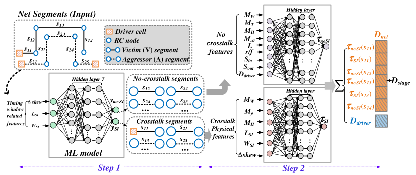
Figure 6. The two-step prediction model for the stage delay (using the MLP as an example).

3.2. Feature Extraction

This part gives the equivalent features for the aforementioned parameters and explains the selection basis for these features. The characteristics and their meanings are summarized in Table 1. Segment length, $L$, has the largest impact on segment delay no matter whether crosstalk exists or not, as shown in Figure 5. To consider the driver cell influence, additional cell delay ($D_{driver}$) features and transition time ($S_{in},S_{out}$) features are extracted using PrimeTime-SI. The driver cell delay is estimated based on the Composite Current Source library. Since its segment delay is estimated by $\tau$, the net delay $D_{net}$ is composed of the no-crosstalk delay and the crosstalk delay, as discussed in Section 3.1.

Table 1. Relevant features for delay prediction.

Feature	Descriptions
Timing information
$\Delta{skew}$	Relative arrival time between nets $i$ and $j$
$r/f(i)$	Input switching direction of current net $i$
$S_{in}(i)$	Input transition of current net $i$
$S_{out}(i)$	Output transition of current net $i$
$D_{driver}(i)$	Pre-predicted driver cell delay of current net $i$
Physical information
$M_{W}$	Interconnect width of current layer
$M_{T}$	Interconnect thickness of current layer
$M_{H}$	Inter-layer-dielectric thickness of current layer
$M_{\varepsilon 0}$	Oxide permittivity of current layer
$L$	The wire length of interconnect
$L_{SI}$	The parallel distance between two segments
$W_{SI}$	The distance between two parallel segments

The capacitance and resistance associated with metal characteristics can be analytically calculated using a variety of physical parameters, as discussed in many parasitic extraction studies (future, ). Among them, directly related factors mainly are the interconnect width, thickness, the permittivity of the oxide, and the inter-layer dielectric thickness, represented by $M_{W}$, $M_{T}$, $M_{H}$, and $M_{\varepsilon_{0}}$, respectively. $M_{W}$, $M_{T}$, $M_{H}$, and $M_{\varepsilon_{0}}$ are disparate for interconnecting segments in various metal layers. Hence, to predict the no-crosstalk delay, additional metal features ($M_{W},M_{T},M_{H},M_{\varepsilon 0}$) are extracted. Furthermore, timing-window-related features ($\Delta{skew},L_{SI},W_{SI}$) are added to represent the crosstalk effect. During routing iterations, these physical characteristics are extracted for more accurate estimation.

3.3. Two-step Prediction Model

The input data is composed of the physical features and delay features of the current interconnect. The output data is the analysis result of stage delay after complete routing, parasitic extraction, and STA flow. For training data generation, the first step is placement with IC Compiler II (ICC2) (ICC, ). Moreover, complete routing with ICC2, parasitic extraction with StarRC, and STA with PrimeTime-SI are also implemented to obtain golden results. To enable crosstalk characterization, PrimeTime-SI output logs are saved to record the crosstalk occured time and the crosstalk-induced delta delay. $W_{SI}$, $L_{SI}$, $\Delta{skew}$ is calculated with C++ scripts based on the PrimeTime-SI results to complete prediction.

Based on the training data, a method for predicting crosstalk-aware stage delay is shown in Figure 6 by employing a two-step model. The first step is crosstalk filtering. Crosstalk segments can be classified in this step. After filtering, the initial set of crosstalk segments is distinguished from those not already eliminated. The next step is to perform delay prediction considering the crosstalk effects on the selected interconnects. The first step not only reduces the data size of segments in the second step but also enhances delay prediction accuracy. Additionally, in order to map from the extracted features to stage delay, multilayer perceptron neural networks (MLP), random forests (RF), XGboost, Keras, and lightGBM are employed. The crosstalk classification task and the delay prediction task are trained independently for each technique. Hyperparameters of all models are carefully tuned by grid-based search for optimizing prediction performance.

Table 2. Experiment benchmarks.

	Benchmarks	#Nets	#gates	Data Size
Train	spi	13474	2404	96MB
	usb_funct	8705	10257	62MB
	des_perf	35684	50546	254MB
	wb_dma	226395	43491	1614MB
	wb_conmax	342868	40089	2445MB
	systemcdes	14133	2514	101MB
Test	tv80	56382	9422	402MB
	aes_core	209462	29655	1493MB
	ac97_ctrl	72485	10166	517MB
	ethernet	27074	37127	193MB
	systemcaes	59817	7314	427MB
Total train		641259	149301	4572MB
Total Test		425220	93684	3032MB

4. Expermental Results

With a foundry 14nm FinFET PDK, 11 designs from the real-world open-source opencore benchmarks are synthesized, placed, and routed as shown in Table 2 (bs, ). The proposed approach is implemented in Python 3.7.11 and trained with PyTorch 1.12 using four NVIDIA Tesla V100 PCIe 32GB GPUs, and then evaluated on a Linux machine with an Intel Xeon Silver 4214 CPU @ 2.20GHz and 252GB memory.

4.1. Two-step Prediction Model

The predicted delay using the proposed two-step model is compared with the PrimeTime-SI analysis results. There are 1.91 million training samples, of which 70% are used for training and 30% for testing. Each model achieves the upper bound of performance on the current experimental platform. Table 3 shows prediction accuracy with five machine learning methods. RF outperforms other models at the first step and lightGBM outperforms others at the second step. The average training time using MLP, XGboost, Keras, RF, and lightGBM is 33.7, 23.1, 25.1, 24.3, and 20.2 minutes, respectively. Due to the observation and analysis above, RF is chosen as the first step model, and lightGBM is the second step model.

Table 3. The prediction accuracy of the first step and the second step on the test designs.

	Model	Prediction accuracy ($R^{2}$ score)
		tv80	aes_core	ac97_ctrl	wb_conmax	systemaes
Step1	MLP	0.9896	0.9895	0.9877	0.9875	0.9896
	XGboost	0.9947	0.9928	0.9968	0.9956	0.9959
	Keras	0.9976	0.9928	0.9958	0.9910	0.9968
	RF	0.9973	0.9960	0.9941	0.9958	0.9975
	lightgbm	0.9976	0.9887	0.9938	0.9956	0.9959
Step2	MLP	0.9735	0.9751	0.9788	0.9750	0.9784
	XGboost	0.9982	0.9960	0.9926	0.9937	0.9989
	Keras	0.9860	0.9776	0.9837	0.9798	0.9906
	RF	0.9830	0.9839	0.9765	0.9825	0.9890
	lightgbm	0.9983	0.9978	0.9966	0.9951	0.9966

Besides, a performance comparison between the proposed two-step model and the one-step model (without the first-step classification) is illustrated in Figure 7. The one-step prediction has a noticeable accuracy loss because the delta delay is not completely consistent with coupling capacitance. In reality, the proportion of crosstalk-critical nets to the total nets in a design is typically small. Since every interconnect is considered a training object in the one-step model, it requires high memory storage.

Figure 7. Comparison the two-step and one-step models.

Table 4. Comparison on prediction performance with “MLCAD22”, “ICCAD20”, and Golden. ($Accuracy={Prediction}\//{Golden}$)

Benchmarks		Accuracy				Runtime(s)
		Golden Flow	ICCAD20 (C20, )	MLCAD22 (22C, )	Ours	Golden Flow			ICCAD20 (C20, )	MLCAD22 (22C, )	Ours
						Route	Extract	STA
Train	spi	1.0000	0.5253	0.6224	0.9969	71	11	19	0.0024	0.0026	0.0271
	usb_funct	1.0000	0.7658	0.6299	0.9966	69	19	21	0.0017	0.0019	0.1471
	wb_conmax	1.0000	0.5840	0.5959	0.9754	241	29	25	0.0026	0.0034	0.1492
	des_perf	1.0000	0.7324	0.7571	0.9967	407	46	44	0.0027	0.0024	0.0543
	wb_dma	1.0000	0.8299	0.7648	0.9966	286	49	32	0.0025	0.0015	0.1531
	systemcdes	1.0000	0.7374	0.8589	0.9967	162	23	24	0.0021	0.0023	0.2431
Test	tv80	1.0000	0.5931	0.6925	0.9932	313	24	29	0.0026	0.0032	0.3372
	aes_core	1.0000	0.4991	0.6828	0.9965	359	22	28	0.0015	0.0045	0.1481
	ac97_ctrl	1.0000	0.4840	0.5607	0.9829	399	23	32	0.0013	0.0033	0.1382
	ethernet	1.0000	0.7399	0.5374	0.9968	263	19	23	0.0023	0.0034	0.153
	systemcaes	1.0000	0.5253	0.5289	0.9779	414	23	22	0.0026	0.0022	0.155
Avg. Train		1.0000	0.6958	0.6898	0.9931	206	30	28	0.0023	0.0024	0.1290
Avg. Test		1.0000	0.5683	0.6004	0.9894	350	22	27	0.0021	0.0033	0.1863

4.2. Delay Prediction Analysis

Performance Metrics: In order to verify the validity of the time window, we evaluate prediction performance with the following three metrics, based on DDR (the delta delay ratio), FSI (the false SI net), and TSI (the true SI net).

• DDR: The delta delay ratio lists the delta delay relative to the stage delay.

• FSI: The false SI net means that the invalid aggressor has coupling capacitances but no overlapping timing windows with the victim net.

• TSI: The true SI net indicates that the effective aggressor has coupling capacitances and overlaps with the victim in timing windows.

A high-density design (aes_core) is conducted under the clock frequency constraint (192Mhz@0.8V) with 80% core utilization. Taking the results from PrimeTime-SI as golden, our model is also compared with two recent works, “ICCAD20”(C20, ) and “MLCAD22”(22C, ). During the evaluation process, features of “ICCAD20” and “MLCAD22” are utilized along with the same prediction method in our model without timing-window-based features. Figure 8 shows the stage delay of some nets from aes_core. Especially, the ring chart shows the components of the delta delay of $n5569$. DDR of $n5569$ is 28.15%, while aggressor nets $n10232$, $n6022$, and $n5952$ are FSIs (gray sectors) and others are TSIs (blue sectors). It demonstrates that FSI can be removed in the first step of our model with the proposed timing-window-related features to avoid prediction pessimism. The effective crosstalk nets filtered by our first-step model are hence less than the total coupling capacitances in general. High wire density will lead to high coupling capacitances, but not also high DDR, vice versa. The higher the DDR of the target net, the more obvious the accuracy improvement. Hence, our approach exhibits better applicability in high-density scenes.

Furthermore, to visualize the performance, Table 4 shows the comparison of our model, “ICCAD20”(C20, ) and “MLCAD22” (22C, ), using routing, parasitic extraction, and STA results as the ground truth. The accuracy of golden results defaults to 1. In this regard, a larger value of accuracy implies better prediction performance. The results in Table 4 show that our model improves prediction accuracy as expected.

Figure 8. Some nets of aes_core. The ring chart shows the components of the delta delay of $n5569$.

4.3. Runtime Analysis

Table 4 shows the runtime of complete post-layout analysis flow (routing, parasitic extraction, and STA) and different machine-learning-based prediction methods. In our model, crosstalk segments are classified in the first step. Only filtered segments need the prediction of delta delay in the second step. When compared to other state-of-the-art approaches, our crosstalk-aware method is a little slower. However, the runtime is acceptable compared to the traditional routing iteration flow so integration into existing routing tools is possible. As a result, the proposed model can serve as an accurate crosstalk-aware timing prediction engine during routing that does not require post-routing information.

5. Conclusion

A timing estimation method is proposed during routing. Using timing-window-related features, our method is more likely to be the post-routing crosstalk-aware timing analysis results. Leveraging machine learning techniques, our approach achieves superior accuracy in estimating crosstalk-aware delay during routing. This work can be integrated into traditional timing-driven routing tools in future to accelerate timing closure.

References

- (1) V Huang, D Shim, H Simka, et al. From interconnect materials and processes to chip level performance: Modeling and design for conventional and exploratory concepts. In IEDM, pages 32–6, 2020. https://dl.acm.org/doi/abs/10.1145/3316781.3317857.
- (2) Leilei Jin et al. A novel delay calibration method considering interaction between cells and wires. In DATE, pages 1–6, 2023. https://ieeexplore.ieee.org/abstract/document/10136932.
- (3) Vidya A Chhabria et al. Xt-praggma: Crosstalk pessimism reduction achieved with gpu gate-level simulations and machine learning. In Proceedings of the ACM/IEEE Workshop on MLCAD, pages 63–69, 2022. https://dl.acm.org/doi/abs/10.1145/3551901.3556483.
- (4) Rongjian Liang et al. Routing-free crosstalk prediction. In Proceedings of the 39th ICCAD, pages 1–9, 2020. https://dl.acm.org/doi/abs/10.1145/3400302.3415712.
- (5) Andrew B Kahng et al. Si for free: machine learning of interconnect coupling delay and transition effects. In SLIP, pages 1–8, 2015. https://ieeexplore.ieee.org/abstract/document/7171706.
- (6) Primetime si: Crosstalk delay and noise., 2022. https://www.synopsys.com/implementation-and-signoff/signoff/primetime.html/.
- (7) Vidya A Chhabria et al. From global route to detailed route: Ml for fast and accurate wire parasitics and timing prediction. In Proceedings of the ACM/IEEE Workshop on MLCAD, pages 7–14, 2022. https://dl.acm.org/doi/abs/10.1145/3551901.3556475.
- (8) Zizheng Guo et al. A timing engine inspired graph neural network model for pre-routing slack prediction. In DAC, pages 1207–1212, 2022. https://dl.acm.org/doi/abs/10.1145/3489517.3530597.
- (9) Erick Carvajal Barboza et al. Machine learning-based pre-routing timing prediction with reduced pessimism. In DAC, pages 1–6, 2019. https://dl.acm.org/doi/abs/10.1145/3316781.3317857.
- (10) Hsien-Han Cheng et al. Fast and accurate wire timing estimation on tree and non-tree net structures. In DAC, pages 1–6, 2020. https://ieeexplore.ieee.org/abstract/document/9218712.
- (11) Ron Ho, Kenneth W Mai, and Mark A Horowitz. The future of wires. Proceedings of the IEEE, 89(4):490–504, 2001.
- (12) Synopsys ic. compiler ii user guide., 2022.
- (13) Opencores., 2021. https://opencores.org/.