Low-Dimensional Projection of Reactive Islands in Chemical Reaction Dynamics Using a Supervised Dimensionality Reduction Method

Abstract

Transition state theory is a standard framework for predicting the rate of a chemical reaction. Although the transition state theory has been successfully applied to numerous chemical reaction analyses, many experimental and theoretical studies have reported chemical reactions with a reactivity which cannot be explained by the transition state theory due to dynamic effects. Dynamical systems theory provides a theoretical framework for elucidating dynamical mechanisms of such chemical reactions. In particular, reactive islands are essential phase space structures revealing dynamical reaction patterns. However, the numerical computation of reactive islands in a reaction system of many degrees of freedom involves an intrinsic challenge—the curse of dimensionality. In this paper, we propose a dimensionality reduction algorithm for computing reactive islands in a reaction system of many degrees of freedom. Using the supervised principal component analysis, the proposed algorithm projects reactive islands into a low-dimensional phase space with preserving the dynamical information on reactivity as much as possible. The effectiveness of the proposed algorithm is examined by numerical experiments for Hénon-Heiles systems extended to many degrees of freedom. The numerical results indicate that our proposed algorithm is effective in terms of the quality of reactivity prediction and the clearness of the boundaries of projected reactive islands. The proposed algorithm is a promising elemental technology for practical applications of dynamical systems analysis to real chemical systems.

I Introduction

The transition state theory (TST) Marcelin (1915); Eyring (1935); Wigner (1937) is a standard framework for explaining and predicting the reactivity and rate of a chemical reaction. The TST is based on two fundamental assumptions: (1) All reactive trajectories pass a surface dividing molecular states into reactant and product states only once during a chemical reaction process (non-recrossing assumption). (2) Reactant molecules are equilibrated in a canonical or microcanonical ensemble (quasi-equilibrium assumption). However, many experimental and theoretical studies Carpenter (1995, 1996); Reyes and Carpenter (1998, 2000); Nummela and Carpenter (2002); Litovitz, Keresztes, and Carpenter (2008); Goldman, Glowacki, and Carpenter (2011); Collins et al. (2013, 2014); Kramer et al. (2015); Carpenter, Harvey, and Orr-Ewing (2016); Hare et al. (2019); Hase (1994); Sun, Song, and Hase (2002); Jayee and Hase (2020); Singleton et al. (2003); Ess et al. (2008); Hare and Tantillo (2017) have reported chemical reactions with a reactivity which cannot be explained by TST due to the breakdown of these assumptions by dynamic effects.

Dynamical systems theory provides a theoretical framework for elucidating chemical reaction mechanisms that TST cannot explain. The dynamical systems approach describes molecular dynamics by trajectories in a phase space spanned by atomic position and momentum coordinates. All reactive trajectories in the phase space are known to pass through the interior of a tubular structure connecting reactant and product regions through a rank-one saddle region during a chemical reaction process Clay Marston and De Leon (1989); De Leon and Clay Marston (1989); de Almeida et al. (1990); De Leon, Mehta, and Topper (1991); Deleon, Mehta, and Topper (1991); De Leon (1992a, b). This tubular structure forms a reactivity boundary, separating the reactive trajectories of the associated reaction channel from the others. Reactive trajectories flow regularly inside the tube in the vicinity of the saddle region, allowing us to define a dividing surface that satisfies the non-recrossing assumption Li et al. (2006); Wiggins et al. (2001); Ezra and Wiggins (2018). Furthermore, the network of reaction tubes corresponding to different reaction channels provides essential information for elucidating chemical reaction mechanisms that violate the quasi-equilibrium assumption of TST Li et al. (2005); Collins et al. (2013, 2014); Katsanikas and Wiggins (2022). The tube connectivity can be captured by reactive island structures—the cross-sections of tubes and their interiors on a surface in the phase space (see Sec. II.1 for details).

Several algorithms have been developed for computing phase space structures in chemical reaction dynamics Kawai and Komatsuzaki (2011); Mancho et al. (2013); Nagahata et al. (2020); Naik, Krajňák, and Wiggins (2021); Mizuno et al. (2021). However, these algorithms have been applied only to model systems with few degrees-of-freedom (DoF) and their efficiency likely deteriorates for real systems with many DoF due to the curse of dimensionality. Therefore, dimensionality reduction techniques for phase space structures are indispensable to practicalize the theoretical framework for elucidating chemical reaction mechanics based on phase space geometry.

Dimensionality reduction techniques have been already applied to chemical reaction dynamics studies, such as ReSPer Tsutsumi et al. (2018, 2020); Tsutsumi, Ono, and Taketsugu (2021) and PathReducer Hare et al. (2019). These existing methods aim to determine low-dimensional representations of molecular structures reflecting structural changes during chemical reactions as much as possible. Such dimensionality reduction tasks are formulated as unsupervised dimensionality reduction in configuration space. However, dimensionality reduction preserving the information of molecular structural changes is not necessarily appropriate for phase space geometry. The information of reactivity of each trajectory should be more essential than that of molecular structures in dimensionality reduction of reaction tubes (i.e., reactivity boundaries). Thus, it is necessary to develop a novel method of determining low-dimensional representations of phase space structures preserving the reactivity information as much as possible. This task can be formulated as supervised dimensionality reduction Chao, Luo, and Ding (2019) in phase space, where supervised data is the reactivity of each trajectory (See Sec. II.2 for details).

In this paper, we propose a method of projecting high-dimensional reactive island structures onto low-dimensional phase space using supervised principal component analysis Barshan et al. (2011). The remainder of this paper is organized as follows. Sec. II introduces the reactive island theory and formulates the dimensionality reduction problem in phase space geometry. Sec. III details our proposed algorithm. Sec. IV presents numerical experiments and performance evaluation of the proposed algorithm applied to a model Hamiltonian system as a proof-of-concept. Finally, the paper is concluded in Sec. V.

II Problem Formulation

II.1 Reactive island theory

Dynamical systems theory of chemical reaction dynamics is based on the phase space picture of molecular dynamics. Let us consider $N$-DoF molecular dynamics in gas phase governed by a Hamiltonian $H$ with potential energy $V$. Molecular states are represented by the atomic positions and momenta of the molecular system, denoted by $(\bm{q},\bm{p})$. Here, $\bm{q}$ and $\bm{p}$ denote the position vector $(q_{1},q_{2},\dots,q_{N})^{\top}$ and the momentum vector $(p_{1},p_{2},\dots,p_{N})^{\top}$, respectively. Each state is represented by a point in the $2N$-dimensional phase space spanned by $\bm{q}$- and $\bm{p}$-axes. Dynamical processes are described by trajectories in the phase space, which never intersect each other. Under an energy conservation condition $H=E\ (\mathrm{const.})$, the energetically accessible region is a $(2N-1)$-dimensional subspace.

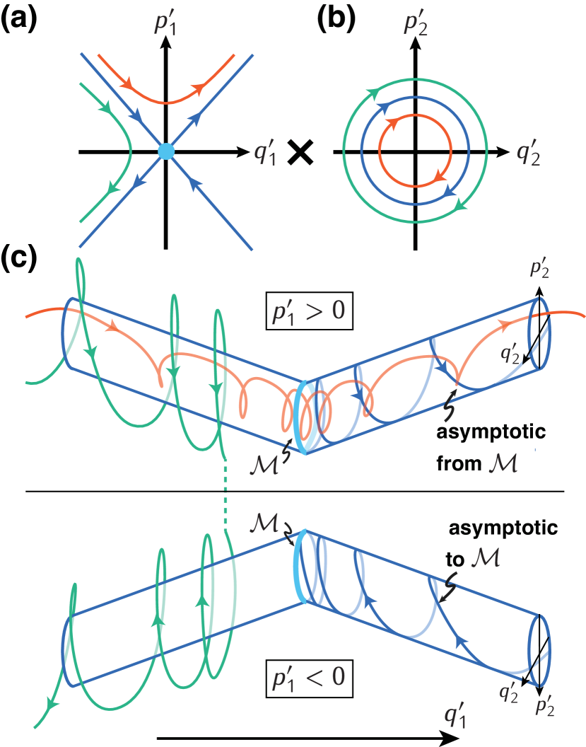
Figure 1: Conceptual illustration of reaction tubes. We consider a 2-DoF Hamiltonian system, though the present discussion can be generalized to any-DoF systems Nagahata, Hernandez, and Komatsuzaki (2021). Near a saddle region, we suppose that the 2-DoF is separated into (a) a reactive mode $q_{1}^{\prime}$ and (b) a thermal bath mode (harmonic oscillator mode) $q_{2}^{\prime}$. Panels (a) and (b) depict trajectories in phase space of the reactive mode and the bath mode, respectively. In panel (a), the red trajectory has sufficient energy in the reactive mode and passes through the saddle region, while the green trajectory has insufficient energy and goes back to the left region. The four blue trajectories take middle positions between them, separating reactive and non-reactive trajectories in the phase space. Given that the total energy is constant, the red trajectory in (a) with large mode energy corresponds to the red trajectory in (b) with small mode energy. Likewise, the green and blue trajectories in (a) also correspond to the trajectories of the same color in (b). Panel (c) schematically depicts the phase space of the 2-DoF system. The blue trajectories exhibit spiral motion consisting of the one-directional motion in (a) and the circular motion in (b). These spiral blue trajectories form tubular structures called reaction tubes, separating reactive (red) and non-reactive (green) trajectories. Note that all reactive trajectories pass through the interior of these tubular structures because they have less energy in the bath mode and lie inside the blue circle in (b). In addition, the light blue origin in (a) and the circular motion in (b) result in an unstable periodic orbit denoted by $\mathcal{M}$ in (c). See also Ref. Nagahata, Hernandez, and Komatsuzaki (2021).

One of fundamental phase space structures for elucidating chemical reactivity is a reaction tube. Figure 1 illustrates the concept of reaction tubes. A reaction tubes is a $(2N-2)$-dimensional cylindrical structure in the phase space, connecting reactant and product regions through a transition state region (i.e., a saddle region of $V$). As illustrated in Fig. 1, a reaction tube forms a reactivity boundary that separates reactive and non-reactive trajectories in the $(2N-1)$-dimensional energetically-accessible subspace; all reactive trajectories pass through the interior of the reaction tube without exception.

Reactive islands provide essential dynamical information to elucidate a reaction system with multiple reaction channels. Figure 2 illustrates the concept of reactive islands. In the figure, we consider a reaction system with two channels A $\to$ B and B $\to$ C. Panel (b) shows the cross sections of the two reaction tubes corresponding to the two reaction channels on a surface $\Sigma$ in panel (a). The cross section of the reaction tubes and their interiors form island-like patterns on $\Sigma$, called reactive islands (RIs). In the present case, the two RIs overlap. This indicates that there exist reactive trajectories directly reacting from A to C without trapped in the intermediate region B. The existence of such bypassing reactive trajectories is known as dynamic matching Carpenter (1995) and neglected in TST due to the quasi-equilibrium assumption. In this way, RIs are crucial for chemical reaction analyses taking into account dynamic effects.

As another example, let us consider a reaction system with three channels, (i)A $\to$ B, (ii)B $\to$ C, and (iii)B $\to$ D. Considering a cross-section $\Sigma$ in the B’s well, there should be three RIs corresponds to the three reaction channels. If the RIs of (i) and (ii) overlap, it indicates that there is the direct reaction path A $\to$ C. Similarly, the overlap of the RIs of (i) and (iii) indicates the existence of the direct reaction A $\to$ D. The selectivity between two products C and D may be estimated by these RI overlapsDe Leon, Mehta, and Topper (1991).

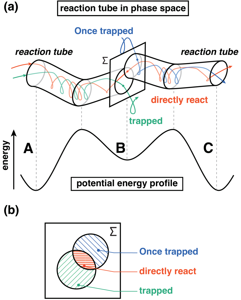
Figure 2: Conceptual illustration of reactive islands. Here, we consider a 2-DoF Hamiltonian system with the potential energy profile shown in panel (a). The potential energy surface has three local minima A, B, and C, corresponding to reactant, intermediate, and product, respectively. In panel (a), reaction tubes of reactions A $\to$ B and B $\to$ C are depicted. The surface designated by $\Sigma$ is a two-dimensional surface at the local minimum B. The surface $\Sigma$ cuts the reaction tubes and the surface of section is shown in panel (b). The intersection of a reaction tube with $\Sigma$ forms a closed curve. The inside of a closed curve consists of intersections of all reactive trajectories with $\Sigma$. This region of the intersections of reactive trajectories enclosed by that of reaction tubes is called reactive island. In the present example, the reactive islands of reactions A $\to$ B and B $\to$ C have overlap. The red trajectory in panel (a) passes the overlap region, indicating that it directly reacts A $\to$ C without trapped in the intermediate region B. In contrast, the green/blue trajectories passing the green/blue reactive island regions in panel (b) are reactive trajectories with trapped in B after/before reactions, respectively. This classification of reactive trajectories is neglected in TST due to the quasi-equilibrium assumption.

II.2 Dimensionality reduction problem

RIs are $(2N-2)$-dimensional structures for an $N$-DoF system; thus a low-dimensional projection of reactive islands is necessary for practical analysis of chemical reaction dynamics with many-DoF. In this subsection, we present a general problem formulation of the dimensionality reduction of RIs. A prototypical algorithm for this problem will be proposed in the next section.

The dimensionality reduction of RIs aims to determine a mapping $f$ from a $(2N-2)$-dimensional surface $\Sigma\ (\subset\mathbb{R}^{2N})$ to a $d$-dimensional space preserving the RI structure as much as possible. Here, $d$ is a user-specified integer number satisfying $d<2N-2$. Note that how to determine $d$ is also a critical issue as well as how to compute $f$. An appropriate protocol of determining $d$ may vary depending on a dimensionality reduction algorithm and a reaction system of interest. We provide a specific protocol for our proposed algorithm in Sec. III and a further perspective in Sec. V. In the remainder of this subsection, we specify the structure of $f$ and measures of the preservation of the RI structure.

We construct the mapping $f$ by composition of a coordinate transformation $\phi$ in the $2N$-dimensional phase space and a projection $\pi$ onto the $d$-dimensional space. Here, the projection $\pi$ is defined as $\pi(z_{1},z_{2},\dots,z_{d},\dots,z_{2N})=(z_{1},z_{2},\dots,z_{d})$. Restricting the domain of $\phi$ to $\Sigma$, we define $f=\pi\circ\phi|_{\Sigma}$. For instance, a dimensionality reduction that projects molecular states onto a subspace spanned by $r$ dominant normal modes can be constructed by the normal mode transformation $\phi$ and a standard projection $\pi$ onto the $2r$-dimensional subspace.

We measure the degree of the RI structure preservation by the dependence between the coordinate variable in the $d$-dimensional subspace and its corresponding reactivity label variable. The reactivity label is, for example, the colored pattern in Fig. 2(b). According to the RI theory, the reactivity label is a dependent variable of the coordinate variable. A dimensionality reduction, however, may map points of different reactivity labels to a single point on the $d$-dimensional subspace. This mixing of reactivity labels decreases the degree of the dependence between the coordinate variable and the reactivity label variable in the $d$-dimensional subspace. In other words, we define the dependence as the relationship that specifying the coordinates determines the reactivity label. This dependence should be conserved as much as possible during a dimensionality reduction as the separation of reactivity is the essence of the concept of RIs.

Therefore, we formulate the dimensionality reduction problem as the following variational problem:

$$\operatorname*{maximize}_{\phi\colon\mathbb{R}^{2N}\to\mathbb{R}^{2N}}\quad \mathcal{D}\left(\bar{\bm{\mathcal{Z}}};\ \mathcal{Y}\right)$$ (1)

subject to $$\bar{\bm{\mathcal{Z}}}=\pi\circ\phi|_{\Sigma}(\bm{\mathcal{Z}})$$

where $\mathcal{D}(\cdot;\cdot)$ denotes a measure of the dependence of two random variables, $\bm{\mathcal{Z}}$ and $\bar{\bm{\mathcal{Z}}}$ signify the coordinate variables in the original phase space and the $d$-dimensional subspace, respectively, and $\mathcal{Y}$ is the reactivity label variable. Several dependence measures can be employed as $\mathcal{D}$, including the Hilbert–Schmidt independence criterion Gretton et al. (2005) and the mutual information. Different classes of the coordinate transformation $\phi$ and different dependence measures $\mathcal{D}$ derive different algorithms for the dimensionality reduction of RIs. The next section presents one of them as a prototypical algorithm.

III Proposed Algorithm

This section presents an algorithm for solving the dimensionality reduction problem given by Eq. (1) using the supervised principal component analysis (SPCA) Barshan et al. (2011). SPCA employs the Hilbert–Schmidt independence criterion (HSIC) Gretton et al. (2005) as the dependence measure $\mathcal{D}$ and restricts the coordinate transformation $\phi$ to orthogonal transformation. The HSIC measures the dependence between two random variables by the Hilbert–Schmidt norm of the cross-covariance operator—the larger HSIC is, the higher the dependence is. For the detailed background of HSIC and SPCA, see the original paper Barshan et al. (2011).

The SPCA algorithm requires a data matrix $\bm{Z}$ and a label matrix $\bm{Y}$ as input. In the present case, the data matrix is a $2N\times m$ matrix whose columns are the $2N$-dimensional coordinate vectors of $m$ points on a surface $\Sigma$. As a preprocessing, all parameters were scaled such that their minimum value is 0 and the maximum value is 1. Then, in the process of SPCA, we assume that the data matrix is centered in advance, that is, the origin of the coordinate vectors is set to their mean. The label matrix is a $1\times m$ matrix where the $m$-th column corresponds to the reactivity label associated with the $m$-th column of $\bm{Z}$. Our proposed algorithm supposes that the reactivity label can be determined using numerical simulation of trajectories initiated from the $m$ points on $\Sigma$. The labeling method may vary depending on a reaction system of interest (see Sec. IV.1 for a specific example).

The orthogonal coordinate transformation $\phi$ and standard projection $\pi$ can be represented by a $2N\times 2N$ orthogonal matrix $\bm{U}$ and a $d\times 2N$ projection matrix $\bm{P}$. Here, the elements of row $i$ and column $j$ of $\bm{P}$ is the Kronecker delta $\delta_{ij}$. The projected data matrix is written as

$$\bar{\bm{Z}}=\bm{P}\bm{U}^{\top}\bm{Z}.$$ (2)

For later convenience, we use $\bm{U}^{\top}$ in Eq. (2) instead of $\bm{U}$.

The HSIC between the projected data and label is empirically estimated from the data as follows:

$$\mathrm{HSIC}=\frac{1}{(2N-1)^{2}}\mathrm{tr}(\bm{KL}).$$ (3)

Here, $\operatorname{tr}$ denotes the matrix trace. The matrix $\bm{K}$ is a data kernel which is written in the present formulation as

$$\bm{K}=\bar{\bm{Z}}^{\top}\bar{\bm{Z}}=\bm{Z}^{\top}\bm{U}\bm{P}^{\top}\bm{P}\bm{U}^{\top}\bm{Z}.$$ (4)

The matrix $\bm{L}$ is a label kernel calculated from the label matrix $\bm{Y}$. In this paper, the entry $l_{i,j}$ is set to 1 if $i$-th data and $j$-th data have the same label, otherwise 0.

The variational problem of Eq. (1) is now given by

$$\operatorname*{maximize}_{\bm{U}\in\mathbb{R}^{2N\times 2N}}\quad \operatorname{tr}(\bm{Z}^{\top}\bm{U}\bm{P}^{\top}\bm{P}\bm{U}^{\top}\bm{Z}\bm{L})$$ (5)

subject to $$\bm{U}^{\top}\bm{U}=\bm{I}.$$

Note that the matrix trace to be maximized is rewritten as

$$\begin{split}&\operatorname{tr}(\bm{Z}^{\top}\bm{U}\bm{P}^{\top}\bm{P}\bm{U}^{\top}\bm{Z}\bm{L})\\ =&\operatorname{tr}\left(\bm{P}(\bm{U}^{\top}\bm{Z}\bm{L}\bm{Z}^{\top}\bm{U})\bm{P}^{\top}\right).\end{split}$$ (6)

Since matrix $\bm{P}$ is a projection matrix, this matrix trace equals to the sum of the first $d$ diagonal elements of matrix $\bm{U}^{\top}\bm{ZLZ}^{\top}\bm{U}$. Given that $\bm{ZLZ}^{\top}$ is symmetric and $\bm{U}$ is an orthogonal matrix, this matrix trace takes the maximum value when the first $d$ columns of $\bm{U}$ are the eigenvectors associated with the top $d$ eigenvalues of $\bm{ZLZ}^{\top}$. Therefore, this optimization problem is reduced to the eigenvalue problem of matrix $\bm{ZLZ}^{\top}$. This reduction is similar to the original (unsupervised) PCA where the empirical sample covariance matrix $\bm{Z}\bm{Z}^{\top}$ is diagonalized through the eigenvalue problem. Indeed, when we set the label kernel $\bm{L}$ to the identity matrix, the SPCA is equivalent to the original PCA. Finally, we summarize the whole procedure of our proposed algorithm as a pseudo code in Fig. 3.

As we mentioned above, how to determine the dimensionality $d$ is one of the important issues. In our framework, we determine $d$ based on the cumulative contribution rate—the ratio of the sum of top $d$ eigenvalues to the sum of all eigenvalues of matrix $\bm{ZLZ}^{\top}$. The larger this value is, the more the dimensionality reduction preserves the dependence between the projected coordinates and its reactivity label. An appropriate value of $d$ can be determined such that the cumulative contribution rate for $d$ is larger than a specified threshold (close to one).

Algorithm 1 Compute a low-dimensional projection of reactive islands

0:  $d$—The diminsionality of a projected space, $m$—The number of samples of initial conditions on a surface $\Sigma$.

0:  $\bar{\bm{Z}}$—Phase space coordinates of $m$ points in the projected space, $\bm{Y}$—Reactivity labels of the $m$ points.

1:  for $i=1$ to $m$ do

2:     $\bm{z}_{i}\leftarrow$ An initial condition sampled on $\Sigma$

3:     $trj_{i}\leftarrow$ A calculated trajectory initiated from $\bm{z}_{i}$

4:     $y_{i}\leftarrow$ The reactivity label of $trj_{i}$

5:  end for

6:  $\bm{z}_{i}$ is scaled to the range 0 to 1 (min-max scaling)

7:  $\bm{z}_{\mathrm{mean}}\leftarrow m^{-1}\sum_{i=1}^{m}\bm{z}_{i}$

8:  $\bm{Z}\leftarrow[\bm{z}_{1}-\bm{z}_{\mathrm{mean}},\dots,\bm{z}_{m}-\bm{z}_{\mathrm{mean}}]$

9:  $\bm{Y}\leftarrow[y_{1},\dots,y_{m}]$

10:  $\bm{L}\leftarrow[\delta_{y_{i},y_{j}}]_{1\leq i\leq m,1\leq j\leq m}$

11:  $\bm{Q}\leftarrow\bm{ZLZ}^{\top}$

12:  $\bm{U}\leftarrow$ The matrix of the eigenvectors of $\bm{Q}$

13:  $\bm{P}\leftarrow$ The projection matrix from $2N$ to $d$ dimension

14:  $\bar{\bm{Z}}\leftarrow\bm{P}\bm{U}^{\top}\bm{Z}$

15:  return  $\bar{\bm{Z}},\bm{Y}$

Figure 3: Pseudo code of the proposed algorithm. This algorithm depends on (1) an initial condition sampler from a surface $\Sigma$, (2) a numerical integration method for the trajectory calculation, (3) a reactivity labeling method, and (4) an eigensolver for $\bm{Q}$, as external subroutines.

IV Numerical demonstration and performance evaluation

This section presents a numerical demonstration of the proposed algorithm. We first define model Hamiltonian systems and numerical procedure in Sec. IV.1. Next, we show projected RIs of the model systems computed by the proposed algorithm in Sec. IV.2. Finally, the performance of the proposed algorithm is evaluated from two different perspective: (1) the quality of reactivity label prediction (Sec. IV.3) and (2) the clearness of reactivity boundary (Sec. IV.4).

IV.1 Model Hamiltonian system and numerical procedure

The model Hamiltonian system that we used is based on the Hénon-Heiles systemHenon and Heiles (1964). The system is a two-DoF Hamiltonian system with one potential minimum and three index-one saddles which define three exit channels to “products.” The 2-DoF Hénon-Heiles Hamiltonian $H_{2}$ is given by

$$H_{2}(q_{1},q_{2},p_{1},p_{2})\\ =\frac{p_{1}^{2}}{2}+\frac{p_{2}^{2}}{2}+\frac{q_{1}^{2}}{2}+\frac{q_{2}^{2}}{2}+q_{1}^{2}q_{2}-\frac{1}{3}q_{2}^{3}.$$ (7)

The potential energy surface of this system is shown in Fig. 4.

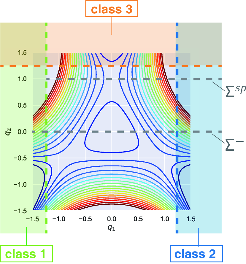
Figure 4: A contour plot of the Hénon-Heiles potential energy landscape. The green, blue, and orange regions are product regions, classes 1, 2, and 3, respectively. The gray dotted lines denote lines (hyperplanes for high-dimensional systems) $q_{2}=0$ ($\Sigma^{-}$) and $q_{2}=1$ ($\Sigma^{\mathrm{sp}}$). In the present numerical demonstration, RIs on the surface $\Sigma^{-}$ were computed, whereas trajectory calculations were started from $\Sigma^{\mathrm{sp}}$. See the text for the detailed calculation procedure.

We extend the two-DoF Hénon-Heiles system to $N$-DoF systems ($N>3$) by adding vibrational bath modes to the original system. The extended $N$-DoF Hénon-Heiles Hamiltonian $H_{N}$ is defined as

$$H_{N}(\mathbf{q},\mathbf{p})=H_{2}+\sum_{i=3}^{N}\frac{1}{2}(p_{i}^{2}+\omega_{i}^{2}q_{i}^{2}+c_{i}q_{2}q_{i}^{2}).$$ (8)

In this paper, we set all frequencies $\omega_{i}\ (i=3,\dots,N)$ to one. All bath modes are coupled with the original $q_{2}$ coordinate and each coupling constant $c_{i}\ (i=3,\dots,N)$ is set to $c_{i}=(-1)^{(i+1)}/2$. This extended $N$-DoF system is designed so that it has one potential energy minimum and three saddle points at the same positions as the original system and that there are no additional equilibrium points in the range of $|q_{i}|\leq 2\ (i=1,\dots,N)$ for $N\leq 10$.

The present numerical demonstration aims to compute RIs on a surface $\Sigma^{-}$ defined as

$$\Sigma^{-}=\left\{(\mathbf{q},\mathbf{p})|q_{2}=0,p_{2}<0,H(\mathbf{q},\mathbf{p})=E\right\}.$$ (9)

This surface traverses the potential minimum $\bm{q}=0$. In particular, we focus on the overlaps between the reaction tube entering the basin around $\bm{q}=0$ through the upper saddle region and those exiting from the basin through the three exit channels. In other words, the present calculation aims to examine whether there exist direct reactive trajectories from class 3 to class 1, 2, or 3 through the intermediate basin region.

To sample data points inside the entering reaction tube efficiently, we sample trajectories initiated from a surface $\Sigma^{\mathrm{sp}}$ defined as

$$\Sigma^{\mathrm{sp}}=\left\{(\mathbf{q},\mathbf{p})\mid q_{2}=1,p_{2}<0,H(\mathbf{q},\mathbf{p})=E\right\}.$$ (10)

This surface traverses the upper saddle point; thus the sampled trajectories are considered as reactive trajectories inside the entering reaction tube. At the saddle point, the reactive mode is mode 2, which is decoupled from the other non-reactive modes. Therefore, we first sample initial conditions for the non-reactive modes $(q_{1},q_{3},...,q_{N},p_{1},p_{3},...,p_{N})$ at uniformly random such that the following condition is met:

$$\frac{1}{2}\left(p_{1}^{2}+3q_{1}^{2}\right)+\sum_{i=3}^{N}\frac{1}{2}\left(p_{i}^{2}+(1+c_{i})q_{i}^{2}\right)\leq E-\frac{1}{6}.$$ (11)

Here, the left and right hand sides correspond to the Hamiltonian of the non-reactive subsystem and the excess energy at the saddle point, respectively. Next, we calculate initial conditions for the reactive mode momentum $p_{2}$ as

$$p_{2}=-\sqrt{2E-\frac{1}{3}-\left\{p_{1}^{2}+3q_{1}^{2}+\sum_{i=3}^{N}\left(p_{i}^{2}+(1+c_{i})q_{i}^{2}\right)\right\}}.$$ (12)

Note that $q_{2}$ is always one on $\Sigma^{\mathrm{sp}}$. Finally, every intersection of a sampled trajectory with $\Sigma^{-}$ is used as a data point $\bm{z}_{i}$.

The reactivity label of each trajectory is determined by the following criterion: A sampled trajectory is labeled as class 1, 2, or 3 if it passes $\Sigma^{-}$ only once and satisfies one of the following conditions within a maximum simulation time $t_{\mathrm{term}}$:

class 1

$q_{1}<-1.25$ (the left green region in Fig. 4)

class 2

$q_{1}>1.25$ (the right blue region in Fig. 4)

class 3

$q_{2}>1.25$ (the upper orange region in Fig. 4)

As we focus on direct reactive trajectories, we label a trajectory as class 0, indicating “not directly reactive”, if the trajectory passes $\Sigma^{-}$ more than once or the simulation time reaches $t_{\mathrm{term}}$ before the above three conditions are met. That is, all intersection points along “not direct reactive” trajectories are labeled as class 0. In this paper, we set $t_{\mathrm{term}}=50$. This value is about eight times longer than the one period of the Hénon-Heiles harmonic oscillator mode $T=2\pi$. Thus the simulation time is considered to be long enough to distinguish direct reactive trajectories from others.

Numerical simulations were conducted for the model systems of 4, 6, 8, and 10 DoFs. The total energy was set so that the average energy for each DoF was 0.1. Therefore, for 4, 6, 8, and 10 DoF systems, the total energy $E$ was set to 0.4, 0.6, 0.8, and 1.0, respectively. A Python program we implemented performed the whole protocol presented above. The trajectory calculation was performed with scipy.integrate.odeint with time step 0.01.

IV.2 Numerical results of the proposed algorithm

Figure 2 shows numerical results for the 8-DoF system. Based on the cumulative contribution rate shown in Fig. 6, we set the dimensionality of the projected subspace $d$ to two for this case. Panels (a) depicts the result of “naive” projection onto the first reactive mode of the original Hénon-Heiles system, and panel (b) displays the results of our proposed algorithm. Here, the naive projection result is shown as a reference for comparison and performance evaluation describe below. While the axes of the naive projection result are the first reactive mode $(q_{1},p_{1})$, those of the SPCA result are superpositions of all reactive and non-reactive modes. Table 1 shows the coefficients of the original position and momentum variables in the top-three principal components (PCs) computed by the SPCA. Additionally, we present results for the 4, 6, and 10-DoF systems in Supplementary Material.

Compared to the RIs projected by the naive projection [Fig. 2 (a)], those projected by our SPCA algorithm [Fig. 2 (b)] appear to be less mixed with other regions; especially, the rightmost part of each projected RI consists of points with the same reactivity. These results indicate the superiority of our SPCA algorithm over the naive projection. In what follows, we will assess the superiority of SPCA in objective manners.

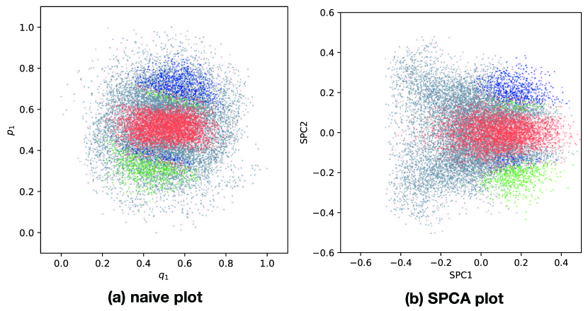
Figure 5: Projected RIs on two-dimensional planes for the 8-DoF Hénon-Heiles system. (a) “naive” projection—data points are projected onto the plane spanned by $q_{1}$ and $p_{1}$. (b) our proposed algorithm—data points are projected onto the plane spanned by the top two principal components computed by the SPCA. The color of each data point indicates the reactivity label of the point—class 0: gray, class 1: green, class 2: blue, and class 3: red.

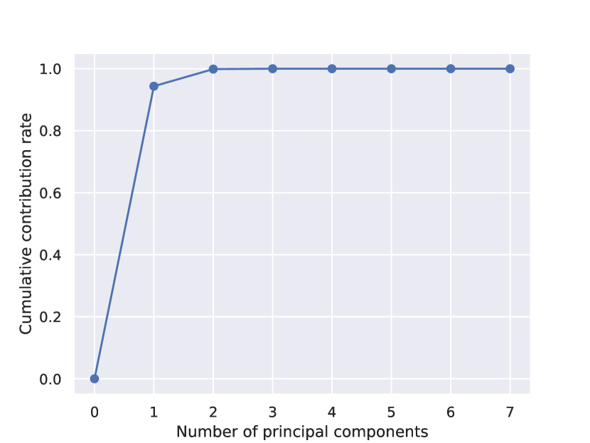
Figure 6: Cumulative contribution rates of the SPCA result for the 8-DoF system. This figure shows the cumulative contribution rate up to the top seven principal components. The top three eigenvalues are $9.4\times 10^{-1}$, $5.6\times 10^{-2}$, $1.1\times 10^{-3}$, while the remaining eigenvalues are less than $10^{-16}$.

Table 1: Compositions of the top-three principal components (PCs) for the 8-DoF system.

	$q_{1}$	$p_{1}$	$q_{2}$	$p_{2}$
PC1	-0.014	-0.0026	0.0	0.99
PC2	-0.34	-0.93	0.0	-0.0060
PC3	0.27	-0.080	0.0	0.044
	$q_{3}$	$p_{3}$	$q_{4}$	$p_{4}$
PC1	-0.0050	-0.014	-0.025	0.015
PC2	0.022	0.028	0.017	-0.014
PC3	0.23	0.13	0.20	-0.28
	$q_{5}$	$p_{5}$	$q_{6}$	$p_{6}$
PC1	-0.0077	0.0012	-0.017	0.013
PC2	0.010	-0.0022	0.010	-0.021
PC3	0.088	-0.38	0.42	-0.24
	$q_{7}$	$p_{7}$	$q_{8}$	$p_{8}$
PC1	0.022	0.0098	0.013	-0.016
PC2	0.0058	0.018	0.016	0.015
PC3	-0.42	-0.35	-0.076	0.12

Table 2 summarizes the ratio of the empirical HSIC of the SPCA result to that of the naive projection result for each model system. As the empirical HSIC is a measure of the dependence between positions on a low-dimensional subspace and reactivity labels, those ratios indicate how much the proposed algorithm preserve the dependence between positions and reactivity labels compared with the naive projection. The table shows that all the ratios are sufficiently large, specifically ranging from about 15 times to 90 times. These large ratios indicate that the proposed algorithm is more effective compared with the naive projection as a dimensionality reduction method for RI calculation. In addition, according to the table, the ratio decreases as $N$ increases. However, this tendency may be improved by more advanced method such as nonlinear kernel dimensionality reduction method. Applying such advanced methods is beyond the scope of this paper and remains as future work.

Table 2: The ratios of the empirical HSICs of the SPCA results to those of the naive projection results for 4, 6, 8, and 10-DoF systems. The ratio value greater than one indicates the SPCA algorithm preserves more information on the dependence between positions and reactivity labels compared to the naive dimensionality reduction.

	4 DoF	6 DoF	8 DoF	10 DoF
HSIC(SPCA/naive)	95	24	18	13

IV.3 Effectiveness evaluation 1: label prediction

An RI pattern provides a predictor of the reactivity label from the phase space coordinate. In particular, the predictor of RIs without dimensionality reduction is a perfect predictor; once we determine an initial condition, we can predict the reactivity of the trajectory starting from the initial condition with 100% accuracy due to the deterministic property of Hamiltonian dynamics. Dimentionality reduction of RIs decreases the prediction accuracy in general, but the degree of the accuracy decrease depends on the dimensionality reduction method. Thus, the quality of the reactivity label prediction is one of the effectiveness indicators of dimensionality reduction methods for RI calculation.

To evaluate the label prediction accuracy, we constructed the k-nearest neighbor predictors Cover and Hart (1967) from the projected labeled data points shown in Fig. 2 and Supplementary Material. A k-nearest neighbor algorithm predicts a reactivity label of a point by majority voting of the labels of the $k$ nearest data points in a low-dimensional space. Here, $k$ is a hyperparameter of the predictor. To predict the labels, the data was divided into training and test sets such that the test data constituted 10% of the total.

Furthermore, we employ the macro-F1 score Manning, Raghavan, and Schütze (2008); Sokolova and Lapalme (2009); Takahashi et al. (2022) as a prediction performance score, which is widely-used for the performance evaluation of multi-class classifiers. The macro-F1 score is based on the F1 score Chinchor (1992) for binary classification between reactivity class $l$ ($l=0,1,2,3$) and the others. The F1 score for the binary classification is defined as

$$F_{1}=\frac{2\cdot\mathrm{Recall}\cdot\mathrm{Precision}}{\mathrm{Recall}+\mathrm{Precision}},$$

where

$$\mathrm{Recall} =\frac{\mathrm{TP}}{\mathrm{TP}+\mathrm{FN}},$$

$$\mathrm{Precision} =\frac{\mathrm{TP}}{\mathrm{TP}+\mathrm{FP}}.$$

Symbols $\mathrm{TP}$, $\mathrm{FP}$, and $\mathrm{FN}$ designate the number of prediction instances of true positive, false positive, and false negative, respectively. Here, ‘positive’ and ‘negative’ indicate a predicted binary label (positive: class $l$, negative: the others), while ‘true’ and ‘false’ indicate whether the prediction is correct or not. The macro-F1 score is the arithmetic mean of the F1 score for each class:

$$\mathrm{macro\mathchar 45\relax}F_{1}=\frac{\sum_{l}F_{1}(\mathrm{class}\;l)}{4}.$$

This value is a scalar quantity uniquely determined for each result of dimensionality reduction. This macro-F1 score is suitable for the performance evaluation of predicting rare reaction events (See Supplementary Material for detailed discussion).

We calculated the ratio of the macro-F1 score for the proposed algorithm to that for the naive projection. The macro-F1 score ratio was calculated for the case of $k=3,5,7,9,11,13$, and $15$ for each-DoF system. The range of the ratio values is between 1.25 and 1.7, thus the macro-F1 ratio is greater than one for all cases. This result shows that the predictive performance of the proposed algorithm is better than the naive dimensionality reduction, irrespective of the choice of the hyperparemeter $k$. For more detailed results, see Supplementary Material.

IV.4 Effectiveness evaluation 2: boundary clearness

RI boundaries are cross-sections of reaction tubes on a phase space surface and specifies a RI pattern. The RI boundary detection is an essential part of efficient algorithms for computing RIs Nagahata et al. (2020); Mizuno et al. (2021). These algorithms (1) estimate provisional RI boundaries from current data points, (2) sample new points from (the vicinity of) the provisional boundaries, and (3) compute the reactivity label of the sampled points based on trajectory calculation. This process refines provisional RI boundaries. Repeating the boundary refinement process, we can compute RI boundaries—thus RI patterns—with satisfactory accuracy.

There are several methods for estimating RI boundaries. The algorithm proposed by Nagahata et al. estimates RI boundaries by the asymptotic trajectory indicator Nagahata et al. (2020). This indicator is based on a fact that the time required for a trajectory to pass through a saddle region increases and diverges to infinity as it approaches a reaction tube. Therefore, long passage time is an indicator of an RI boundary. The algorithm proposed by Mizuno et al. estimates RI boundaries by Voronoi tessellation of labeled data points. This boundary detection method is based on a simple fact that RI boundaries separate regions with different reactivity labels.

The dimensionality reduction of RIs blurs RI boundaries in general. For example, as shown in Fig. 2, different-reactivity points are mixed in some areas on the low-dimensional space, making “fuzzy” RI boundaries. This fuzziness of projected RI boundaries makes the aforementioned boundary refining process less efficient. Thus, the clearness of reactivity boundaries is one of the effectiveness indicators of dimensionality reduction methods for RI calculation. In the remainder of this subsection, we compare reactivity boundaries projected by the proposed algorithm and the naive projection based on the two criteria, (1) reactivity label separation (employed by Mizuno et al. Mizuno et al. (2021)) and (2) trajectory passage time (employed by Nagahata et al. Nagahata et al. (2020)).

IV.4.1 Reactivity label separation

RI regions projected onto a low-dimensional space can be estimated based on a predicted probability $p(l|x)$ that the reactivity label is $l$ at point $x$ on the projected space Mizuno et al. (2021). The probability $p(l|x)$ can be viewed as the grade of membership of $x$ in the RI of $l$ as a fuzzy set.

To visualize the fuzziness of projected RIs, we plotted heatmaps of the following indicator $C$:

$$C(x)=\max_{l\in\{1,2,3\}}p(l|x).$$ (13)

This value indicates the certainty (or purity) of RI attribution at point $x$. Figure 7 shows the results for the proposed algorithm and the naive projection.

In the SPCA case, red grids with high $C$ value form clusters, each of which corresponds to an RI. The surrounding areas of the red clusters with color gradation from red to blue correspond to fuzzy RI boundaries. On the other hand, there are few red grids and the color gradation corresponding fuzzy RI boundaries—especially for classes 1 and 2—is unclear in the naive projection case. As noted in the beginning of this subsection, efficient algorithms Nagahata et al. (2020); Mizuno et al. (2021) compute RI boundaries by sampling data points in the vicinity of provisional boundaries. In other words, these algorithms save the cost of computing data points with high-confidence label estimates, i.e., high $C$ values in the present case. Since grids with high $C$ values are more clearly separated from fuzzy RI boundary regions in the SPCA case than in the naive projection case, the SPCA-based projection should be more suitable for applying the efficient algorithm for RI calculation. These results suggest that the proposed algorithm using SPCA is more effective than the naive projection in terms of the clearness of fuzzy RI boundaries.

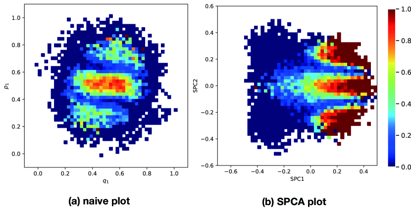
Figure 7: Heatmaps of the certainty of RI attribution [Eq. (13)] for the 8-DoF system. To plot the heatmaps, we divided each low-dimensional space into grids and estimated the probability $p(l|x)$ by the ratio of label $l$ among the data points in the grid of point $x$. This heatmaps are calculated from 17073 data points.

IV.4.2 Trajectory passage time

The passage time of a trajectory through a saddle region is an indicator of a RI boundary Nagahata et al. (2020). Figures 8 (a) and (b), respectively, depict the data points in Figs. 2 (a) and (b) with color brightness indicating the passage time. In Fig. 8, the passage time is defined as the time to hit the classification condition described in Sec. IV.1 for each trajectory starting from $\Sigma^{\mathrm{sp}}$. We also show magnified views of the central regions of class 3 in panels (c) and (d) to make the brightness distribution and gradient clear.

In the SPCA case [panels (b) and (d)], bright points with long trajectory passage time accumulate around the boundary of each color cluster. Such bright points likely correspond to RI boundaries. On the other hand, bright points scatter inside each color cluster in the naive projection case [panels (a) and (c)]. These results also support that the proposed algorithm is an effective way to capture RI boundaries compared with the naive projection.

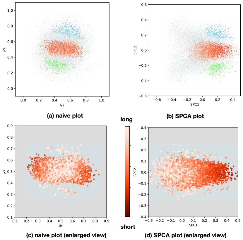
Figure 8: Projected RIs on two-dimensional planes with color brightness indicating trajectory passage time. The data points are the same as those shown in Fig. 2. The color of each data point indicates the reactivity label of the point—class 0: gray, class 1: green, class 2: blue, and class 3: red. The color brightness indicates the trajectory passage time; brighter colors represent longer passage times. Note that the scale of the brightness gradation is determined for each class. Furthermore, to clarify the location of the projected RI boundaries corresponding to bright color points, the points are plotted so that the brighter points are more in the foreground. Panels (c) and (d) are magnified views of red points (class 3) in the central part of panels (a) and (b), respectively.

V Concluding remarks

We have formulated the dimensionality reduction problem of RIs and developed an algorithm to solve the problem using SPCA. The effectiveness of the proposed algorithm was examined by numerical experiments for many-DoF Hénon-Heiles systems. The numerical results indicate that our proposed algorithm is effective in terms of the quality of reactivity prediction and the clearness of projected RI boundaries, compared with the naive projection method.

The algorithm proposed in this paper is a prototype of dimensionality reduction algorithms for numerical phase space geometry. Although the SPCA employed in the present study is a linear dimensionality reduction method, the SPCA can be extended to nonlinear dimensionality reduction method with kernel trick Schölkopf and Smola (2002). Moreover, there are other supervised dimensionality reduction techniques, such as partial least squares Wold (1975), canonical correlation analysis Hotelling (1936), and UMAP McInnes, Healy, and Melville (2018). Applying these methods may enhance the effectiveness of the dimensionality reduction of RIs. In addition, focusing on clustering rather than just dimensionality reduction could lead to an interesting development in discussing reactive islands. The research of Wiggins et al.  Naik, Krajňák, and Wiggins (2021) would be informative in this regard.

Systematic methods for determining appropriate dimensionality $d$ of projection should also be developed. In the present study, we determined $d$ based on the cumulative contribution rate. However, this is not the unique choice for determining $d$. For instance, we can adopt residual variance Tenenbaum, De Silva, and Langford (2000) as another criterion for this purpose. Model selection criteria such as AICAkaike (1974) and BICSchwarz (1978) and sparse modeling techniques Zou, Hastie, and Tibshirani (2006); Adachi and Trendafilov (2016) may also be applicable to the determination of $d$. Appropriate model selection methods for numerical phase space geometry remain open for further investigation.

The final goal of numerical phase space geometry is to elucidate dynamical reaction mechanisms of real chemical systems. Although the present study employs model Hamiltonian systems for the proof of concept, our algorithm does not assume analytical expressions of Hamiltonian. Therefore, the proposed algorithm can be combined with ab initio molecular dynamics calculation to compute projected RIs in real molecular systems. Additionally, one can integrate the dimensionality reduction algorithm with the efficient trajectory sampling algorithms for computing RIs Nagahata et al. (2020); Mizuno et al. (2021) (see also Sec. IV.4). Although the curse of dimensionality in computing phase space structures can be mitigated by dimensionality reduction techniques, the required number of trajectory calculation may still be too large to apply the algorithm to real molecular systems of many-DoF. This issue may be resolved by using a neural network potential Manzhos and Carrington (2021) as a surrogate model for molecular dynamics simulation. We expect that the further development of numerical methods for phase space geometry and their application to real chemical systems will practicalize and facilitate the dissemination of chemical reaction analysis from the point of view of dynamical systems theory.