Scalable and Robust Transformer Decoders for Interpretable Image Classification with Foundation Models

Abstract

Interpretable computer vision models can produce transparent predictions, where the features of an image are compared with prototypes from a training dataset and the similarity between them forms a basis for classification. Nevertheless these methods are computationally expensive to train, introduce additional complexity and may require domain knowledge to adapt hyper-parameters to a new dataset. Inspired by developments in object detection, segmentation and large-scale self-supervised foundation vision models, we introduce Component Features (ComFe), a novel explainable-by-design image classification approach using a transformer-decoder head and hierarchical mixture-modelling. With only global image labels and no segmentation or part annotations, ComFe can identify consistent image components, such as the head, body, wings and tail of a bird, and the image background, and determine which of these features are informative in making a prediction. We demonstrate that ComFe obtains higher accuracy compared to previous interpretable models across a range of fine-grained vision benchmarks, without the need to individually tune hyper-parameters for each dataset. We also show that ComFe outperforms a non-interpretable linear head across a range of datasets, including ImageNet, and improves performance on generalisation and robustness benchmarks.

Figure 1: Illustration of ComFe. Image is clustered into component features, from which the salient parts for predicting the class Scarlet tanager are identified. These can then be cross-referenced to the training data to explain the prediction.

1 Introduction

From identifying disease in medical imaging [68], to species identification [4] and self-driving cars [29], deep learning is used in numerous contexts to solve computer vision problems. However, standard deep learning approaches are black boxes [49], and it can be challenging to determine when a prediction is being made based on the most relevant features in an image. For example, neural networks can often learn spurious correlations from image backgrounds[65].

Post-hoc interpretability techniques can uncover this behaviour, such as class activation maps [67], and recent advances have considered neural network architectures that provide explainability using attention maps [46] or other specialised features [25]. However, these approaches are not transparent in that they cannot be used to understand which parts of the training dataset might be leading to these relationships. Interpretable models, that are designed to reason in a logical fashion, can achieve this goal by identifying prototypical parts within a training dataset that provide evidence for a particular category [8, 40, 62].

Nevertheless, interpretable models can have a poor semantic correspondence between the embeddings of prototypes and their visual characteristics [26, 21], which is a problem that crosses over into the field of self-supervised learning (SSL). SSL techniques use an optimisation task defined by the data itself to train models such as neural networks, and in the computer vision space these models have shown an impressive ability to create an embedding space that reflects semantic similarity [9, 11, 10]. Recent advances in this area have lead to the development of foundation models that can produce useful embeddings across a range of different vision tasks, such as DINOv2 [43] and CLIP [47, 13].

To take advantage of these developments we present Component Features (ComFe), a novel explainable image classification approach that uses the components of an image identified by a transformer decoder [57] to make explainable predictions. As shown in Fig. 1, ComFe is able to identify the relevant patches within an image, the class they represent, and cross-reference the embeddings of these features with the training dataset to answer why a particular prediction is made. This approach is inspired by the Detection Transformer [7], Mask2Former [12] and PlainSeg [22], in addition to recent advances in semi-supervised learning [2, 39, 35]. In this paper, we demonstrate that

1. ComFe produces segmentation maps for the regions of an image that relate to the class prediction.

2. ComFe produces segmentation maps for component features, which are able to consistently detect particular regions of an image (e.g. a birds head, body and wings), and can be used to identify the training examples relevant to a prediction.

3. ComFe is scalable to image datasets with large numbers of training examples and classes, such as ImageNet [50].

4. ComFe obtains superior performance to previous interpretable modelling approaches, and can also outperform a non-interpretable linear head across a range of benchmarking datasets.

5. ComFe is more generalisable and robust in comparison to a non-interpretable linear head.

2 Related work

2.0.1 Interpretable vision models.

ProtoPNet [8] was the first method to show that deep learning computer vision models could be designed to explain their predictions and obtain competitive performance compared to non-interpretable approaches. They introduced prototypes for explainability, visual representations of concepts from the training data that can be used to explain a model’s prediction. ProtoPNet learns a fixed number of prototypes per class, and to make a classification it calculates the similarity between the set of prototypes and the patches within an image. Similarity is measured using a distance metric between the embeddings of the prototype and image patch within a latent or representation space, defined by their mapping under a neural network. Further work, including ProtoTree [41], ProtoPShare [52], ProtoPool [51], ProtoPFormer [62] and PIP-Net [40] improve on this approach. However, these methods are computationally expensive, require domain knowledge to adapt the model hyperparameters to a new dataset, and are increasingly complex [46]. In contrast, the recent INTR [46] approach uses the cross-attention layer from a transformer decoder head to produce explanations of image classifications. While elegant, this moves away from training data prototypes, making these models less transparent than the ProtoP family.

2.0.2 Prototypical learning approaches.

Prototypical deep learning methods learn a mapping from the input data to a metric or semi-metric space, where classification is performed by determining the distance of new inputs to a set of prototypical representations of each class [54]. Interpretable vision models that use a distance metric between prototypes and image patches are a form of prototypical learning, and other work has found prototypical approaches beneficial in improving out-of-distribution detection [38, 33], out-of-distribution generalisation [3] and semi-supervised learning [2, 39, 35]. They have also been used to improve model robustness [63], for few-shot learning [54] and also in multi-model applications [47].

2.0.3 Self-supervised learning and foundation models.

In computer vision, self-supervised approaches train neural networks as functional mappings between the image domain and a representation or latent space that captures the semantic information contained within the image with minimal loss. State-of-the-art self-supervised approaches can obtain competitive performance on downstream tasks such as image classification, segmentation and object detection when compared to fully supervised approaches [56, 43]. This is achieved by using techniques such as bootstrapping [17], masked autoencoders [18], or contrastive learning [9], which use image augmentations to design losses that encourage a neural network to project similar images into similar regions of the latent space. By combining these approaches on large scale datasets, foundation models such as DINOv2 [43] can be trained that perform well across a range of visual contexts. Language-image pretraining can also be an effective self-supervised approach, but requires large image datasets with captions to train models [47, 13].

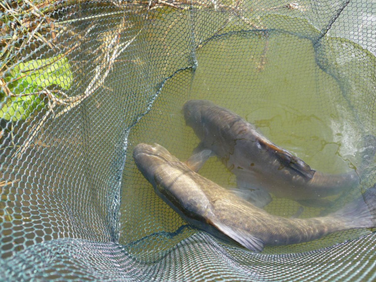
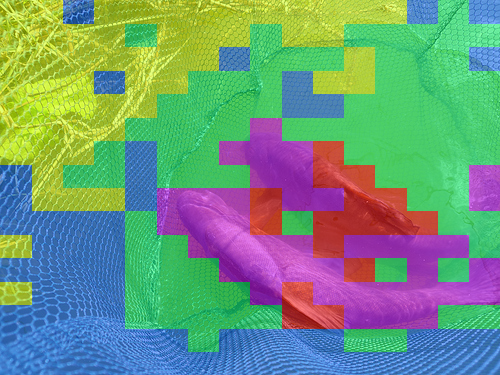
Figure 2: Example of image overlayed with $k$-means clustering on normalised DINOv2 patch embeddings.

Figure 3: The ComFe modelling framework. The double slashed arrow indicates gradients are not propogated to the model backbone.

3 Methodology

3.0.1 Motivation.

The patch features obtained from foundation models like DINOv2 are highly informative. They define a semi-metric space, where the cosine similarity between image patches determines their degree of semantic similarity. For example, in Fig. 2 simple $k$-means clustering on the normalised DINOv2 patch embeddings can easily segment the fish from the background. Given this, we ask can a model be trained on this feature space that explicitly localises predictions based on context clues? For image classification, these context clues are the global image labels.

We take a hierarchical mixture modelling [36, 69] approach to solving this problem. We cluster the image patches into component features using image prototypes, and then cluster the image prototypes into class prototypes that inform how the image should be classified. This enforces a reasoning process using the semi-metric space of the foundation model as shown in Fig. 3, where image patches with similar embeddings are grouped to represent image components (e.g. a cat’s head), which are then clustered using class prototypes to identify the class-informative portion of the image.

3.0.2 Notation.

We refer to an image as $\textbf{X}\in\mathbb{R}^{3\times h\times w}$, where $w$ is the image width and $h$ is the height. Throughout this paper, we use bolded characters to refer to matrices or arrays, and the notation $\textbf{X}_{i:}$ refers to the $i^{\text{th}}$ row. The respective lowercase letter with two subscripts $x_{ij}$ refers to a specific element of the matrix X. We employ a frozen foundation model $f$ and a head network $g_{\theta}$ to make predictions, where $\theta$ refers to the model parameters.

3.0.3 Modelling framework.

Consider the embeddings of a matrix of image patches, $\textbf{Z}=f(\textbf{X})\in\mathbb{R}^{N_{Z}\times d}$ as provided by the backbone foundation model $f$, and a matrix of image prototypes $\textbf{P}\in\mathbb{R}^{N_{P}\times d}$, where $N_{P}$ is the number of image prototypes and $d$ is the dimensionality of the representation space. Each patch has a class $y$, which we can define the joint probability as

$$p(\textbf{Z}_{i:},\textbf{P}_{j:},y): =p(\textbf{Z}_{i:}|\textbf{P}_{j:})p(\textbf{P}_{j:}|y)p(y)$$ (1)

where $p(y)$ is the prior distribution for the classes. Here, the image prototype $\textbf{P}_{j:}$ acts as a latent variable that relates the image patch $\textbf{Z}_{i:}$ to the class $y$ using a generative approach.

We parameterise these distributions using the following mixture model,

$$p(\textbf{Z}_{i:}|\textbf{P}_{j:}): =k(\textbf{Z}_{i:},\textbf{P}_{j:};\tau_{1})$$ (2)

$$p(\textbf{P}_{j:}|y): =\sum_{l}^{N_{C}}\phi_{ly}k(\textbf{P}_{j:},\textbf{C}_{l:};\tau_{2})$$ (3)

$$k(\textbf{Z}_{i:},\textbf{P}_{j:};\tau_{1}): =C_{d}\left(\frac{1}{\tau_{1}}\right)\exp\left(\frac{1}{\tau_{1}}\frac{\textbf{Z}_{i:}.\textbf{P}_{j:}}{||\textbf{Z}_{i:}||||\textbf{P}_{j:}||}\right)$$ (4)

where $k$ is a von-Mises Fischer distribution with normalising constant $C_{d}$ and concentration defined by the temperature parameters $\tau_{1}$ and $\tau_{2}$. We consider $N_{C}$ components to the mixture model that describes the relationship between the image prototypes $\textbf{P}_{j:}$ and the classes $y$, where the membership of each mixture component to each class is described by the smoothed one-hot encoded matrix $\bm{\phi}\in\mathbb{R}^{N_{C}\times c}$

$$\phi_{ly}: =1-\alpha+\frac{\alpha}{c}\text{ if }(j\mod\frac{N_{C}}{c})=y\text{ else }\frac{\alpha}{c}$$ (5)

where $\alpha$ is the smoothing parameter and $c$ is the number of classes.

3.0.4 Predicting patch class membership.

We can use Bayes’ rule to obtain the probability that a patch belongs to a particular class under this model, assuming that the prior distributions for the image prototypes $p(\textbf{P}_{j:})$ and the classes $p(y)$ are uniform. First, we consider the probably that a patch $\textbf{Z}_{i:}$ was generated by a specific image prototype $\textbf{P}_{j:}$

$$p(\textbf{P}_{j:}|\textbf{Z}_{i:}) =\frac{p(\textbf{Z}_{i:}|\textbf{P}_{j:})p(\textbf{P}_{j:})}{p(\textbf{Z}_{i:})}$$ (6)

$$=\sigma\left(\hat{\textbf{Z}}_{i:}.\hat{\textbf{P}}/\tau_{1}\right)_{j}$$ (7)

where $\sigma$ is the softmax function. We may compute the probability that an image prototype $\textbf{P}_{j:}$ was generated by a particular class $y$ using the same approach

$$p(y|\textbf{P}_{j:}) =\frac{p(\textbf{P}_{j:}|y)p(y)}{p(\textbf{P}_{j:})}$$ (8)

$$=\sigma\left(\hat{\textbf{P}}_{j:}.\hat{\textbf{C}}/\tau_{2}\right)\bm{\phi}_{:y}$$ (9)

which allows us to determine the probability of a particular class $y$, given patch $\textbf{Z}_{i:}$ through

$$p(y|\textbf{Z}_{i:}) =\sum_{j}^{N_{P}}p(y|\textbf{P}_{j:})p(\textbf{P}_{j:}|\textbf{Z}_{i:})$$ (10)

where the image prototypes $\textbf{P}_{j:}$ are introduced as a latent variable which relates the two variables, and then marginalised from the expression.

3.0.5 Deriving the Training objective.

We wish to maximise the log-likelihood of our model, however we do not know the patch level labels $y$. Instead, we consider the image level label $\nu$, which we view as a one-hot encoded class vector. The probability of a class being present within an image can be defined as the maximum class probability over all image patches, creating a vector of Bernoulli distributions, of which the $l^{\text{th}}$ element is given by

$$p(\nu_{l}|\textbf{Z}): =\max_{i}p(y=l|\textbf{Z}_{i:})$$ (11)

Using this approach, the log likelihood for our model for a single image is

$$\log p(\textbf{Z},\nu) =\sum_{l}^{c}\log p(\nu_{l}|\textbf{Z})+\log p(\textbf{Z})$$ (12)

where the clustering portion of the loss is given by the marginal distribution

$$L_{\text{cluster}} =\log p(\textbf{Z})$$ (13)

$$=\frac{1}{N_{Z}}\sum_{i}^{N_{Z}}\log p(\textbf{Z}_{i:})$$ (14)

$$=\frac{1}{N_{Z}}\sum_{i}^{N_{Z}}\log\sum_{j}^{N_{P}}p(\textbf{Z}_{i:}|\textbf{P}_{j:})p(\textbf{P}_{j:})$$ (15)

$$=\frac{1}{N_{Z}}\sum_{i}^{N_{Z}}\log\sum_{j}^{N_{P}}k(\textbf{Z}_{i:},\textbf{P}_{j:};\tau_{1})+C$$ (16)

with the constant $C$ resulting from the uniform prior on the image prototypes $\textbf{P}_{j:}$. Finally, the discriminative portion is given a binary cross entropy loss

$$L_{\text{discrim}} =\sum_{l}^{c}\log p(\nu_{l}|\textbf{Z})$$ (17)

$$=\sum_{l}^{c}\nu_{l}\log p(\nu_{l}=1|\textbf{Z})+(1-\nu_{l})\log(1-p(\nu_{l}=0|\textbf{Z}))$$ (18)

3.0.6 Auxilary loss.

We add three additional constraints to the model to improve model quality using an auxilary loss term $L_{\text{aux}}$. For the first constraint, we observe that through Eq. 10 we have

$$p(\nu_{l}|\textbf{Z}) \leq p(\nu_{l}|\textbf{P})$$ (19)

where

$$p(\nu_{l}|\textbf{P}): =\max_{j}p(y=l|\textbf{P}_{j:})$$ (20)

We find that adding an additional discriminative loss term to maximise this probability using binary cross entropy

$$L_{\text{p-discrim}}: =\sum_{l}^{c}\log p(\nu_{l}|\textbf{P})$$ (21)

$$=\sum_{l}^{c}\nu_{l}\log p(\nu_{l}=1|\textbf{P})+(1-\nu_{l})\log(1-p(\nu_{l}=0|\textbf{P}))$$ (22)

results in a small performance improvement.

To ensure that the image and class prototypes have no redundancy, we add a second term to ensure the image prototype vectors and the class prototype vectors are unique. We achieve this by using a contrastive loss term [9]

$$L_{\text{contrast}} =-\sum_{i}^{N_{c}}\log\frac{\exp(\textbf{C}_{i:}.\textbf{C}_{i:}/\tau_{c})}{\sum_{j}^{N_{c}}\exp(\textbf{C}_{i:}.\textbf{C}_{j:}/\tau_{c})}-\sum_{i}^{N_{P}}\frac{\exp(\textbf{P}_{i:}.\textbf{P}_{i:}/\tau_{c})}{\sum_{j}^{N_{P}}\exp(\textbf{P}_{i:}.\textbf{P}_{j:}/\tau_{c})}$$ (23)

with the temperature parameter $\tau_{c}$. We note that this constraint is not memory intensive, as the contrastive loss is defined between the prototypes that belong to a particular image.

The third constraint encourages consistency in the prototypes assigned to particular patches when the image is augmented. We use a loss term inspired by Consistent Assignment for Representation Learning [40, 53] (CARL)

$$L_{\text{CARL}} =-\frac{1}{N_{Z}}\sum_{i}^{N_{Z}}\sum_{j}^{N_{P}}\log p(\textbf{P}_{j:}|\textbf{Z}_{i:})p(\textbf{P}_{j:}^{*}|\textbf{Z}_{i:}^{*})$$ (24)

where $\textbf{Z}^{*}$ and $\textbf{P}^{*}$ are the patch embeddings and image prototypes from an augmented view $X^{*}$ of the image $X$. This loss term is minimised when the softmax vectors given by Eq. 7 from different views are consistent and confident. To create the augmented views we apply the same cropping and flipping augmentations, so that the patches cover the same image region, but different color and blur augmentations.

Our final auxiliary loss term is given by adding these three component terms.

$$L_{\text{aux}} =L_{\text{p-discrim}}+L_{\text{contrast}}+L_{\text{CARL}}$$ (25)

which fully specifies the complete training objective for a single image, given by

$$L =L_{\text{cluster}}+L_{\text{discrim}}+L_{\text{aux}}$$ (26)

When fitting the log-likelihood over more than one image, we using a mini-batch approach and use the average log-likelihood over the batch as our optimisation loss.

3.0.7 Fitting the prototypes.

We consider the class prototypes C as a matrix of learnable parameters, while the image prototypes P are fit parametrically. For each image, we generate the image prototypes using a transformer decoder $g_{\theta}$ [57]

$$\textbf{P}_{i:}=g_{\theta}(\textbf{Z},\textbf{Q}_{i:})$$ (27)

where $\textbf{Q}\in\mathbb{R}^{N_{P}\times d}$ is a learnable query matrix, that prompts the decoder to calculate the image prototypes by considering the entire patch representation of the image Z.

3.0.8 Background classes.

To allow the model to learn non-informative patches, we add an additional background class and assume that each image has atleast one background patch. This turns a multi-class image classification problem into a multi-label one, where we add the background class to the label for each image and $N_{N}$ additional background class prototypes

$$\nu_{w/b} =\left[\nu,1\right]$$ (28)

$$\bm{\phi}_{w/b} =\left[\left[\bm{\phi}>\frac{\alpha}{c},0\right],\left[e_{c+1}\right]\times N_{N}\right](1-\alpha)+\frac{\alpha}{c+1}$$ (29)

where $e_{i}\in\mathbb{R}^{c+1}$ is a unit vector with one in the $i^{\text{th}}$ position. We also extend C to obtain $\textbf{C}_{w/b}\in\mathbb{R}^{N_{C}+N_{N}\times d}$.

This can be done without changing the form of the discriminative loss terms in Eq. 18 and Eq. 22 as binary cross-entropy loss is designed to be used for multi-label classification problems.

3.0.9 Comparison to closely related work.

The ComFe head shares a similar architecture to the INTR [46] approach, in that they both use a transformer decoder on the outputs of the backbone network to make a prediction. However, INTR uses the query Q to define classes and relies on cross-attention within the decoder heads to interpret why the model is making a particular prediction. For ComFe, the query has a fixed size that does not depend on the number of classes and we use the semi-metric space defined by the frozen backbone model and cosine similarity to image P and class C prototypes to explain the model outputs. This makes ComFe much more scalable, allowing us to easily fit models on ImageNet with a single GPU.

4 Experiments

4.1 Implementation details

The weights of our backbone model $f$ are frozen during training, and the parameters of the transformer decoder are randomly initialized. We also randomly initialise our queries Q and class prototypes C. We use the AdamW optimiser [32], cosine learning rate decay with linear warmup [31, 16] and gradient clipping [37]. For image augmentations, we follow DINOv2 and other works, including random cropping, flipping, color distortion and random greyscale [9, 43].

For the architecture of the ComFe head, we use two transformer decoder layers with eight attention heads. We calculate the loss after each decoder layer and take gradients on the average [22]. We feed the output of the last layer of the backbone model directly into the transformer decoder, which results in a higher input dimension in comparison to other works [46], but we find that this gives best results. We use a total of five image prototypes (which means Q will have five rows), and $6c$ class prototypes C. The first $3c$ class prototypes are assigned to each class (for three per class), while the remaining $3c$ are assigned to the background class. We use similar temperature parameters to previous works [2], with $\tau_{1}=0.1$, $\tau_{2}=0.02$ and $\tau_{c}=0.02$.

The same set of hyperparameters are used across all of the training runs, with the exception of the batch size which we increase from 64 images to 1024 for the ImageNet dataset. We also reduce the number of epochs for ImageNet [50], from 50 epochs per a training run to 20 epochs. Training on ImageNet with the ViTS model takes around 21 hours, and for the ViTL model around 35 hours with a 80GB Nvidia A100 GPU. Smaller datasets such as Oxford Pets [45] take less than fifteen minutes. For the ViTS model, a batch size of 64 requires around 2GB of GPU memory, and a batch size of 1024 requires 20GB of GPU memory. While there is the potential for pretraining on a dataset with ComFe by dropping the discriminative loss, we have not found that this is necessary to obtain good performance. Further details on the hyperparameters will be available in the codebase released publicly on GitHub.

4.2 Datasets

Finegrained image benchmarking datasets including Oxford Pets (37 classes) [45], FGVC Aircraft (100 classes) [34], Stanford Cars (196 classes) [27] and CUB200 (200 classes) [61] have all previously been used to benchmark interpretable computer vision models. We use these to test the performance of ComFe, in addition to other datasets including ImageNet-1K (1000 classes) [50], CIFAR-10 (10 classes), CIFAR-100 (100 classes) [28], Flowers-102 (102 classes) [42] and Food-101 (101 classes) [6]. These cover a range of different domains and have been previously used to evaluate the linear fine-tuning performance of the DINOv2 models [43].

We also consider a number of different test datasets for ImageNet that are designed to measure model generalisability and robustness. ImageNet-V2 [48] follows the original data distribution but contains harder examples, Sketch [59] tests if models generalise to sketches of the ImageNet class and ImageNet-R [19] tests if models generalise to art, cartoons, graphics and other renditions. Finally, the ImageNet-A [20] test dataset consists of real-world, unmodified and naturally occuring images of the ImageNet classes that are often misclassified by ResNet models. While ImageNet-V2 and Sketch contain all of the ImageNet classes, ImageNet-A and ImageNet-R only provide images for a 200 class subset.

4.3 Main results

Table 1: Performance of ComFe and other interpretable image classification approaches on several benchmarking datasets, with non-interpretable baselines.

	Head		Backbone		Dataset
					CUB	Pets	Cars	Aircr
Non-interpretable	Linear [46]		ResNet-50	26M	83.8	89.5	89.3	80.9
	Linear [43]		DINOv2 ViT-S/14 (f)	21M	88.1	95.1	81.6	74.0
Interpretable	ProtoPNet [8]		ResNet-34	22M	79.2		86.1
	ProtoTree [41]		ResNet-34	22M	82.2		86.6
	ProtoPShare [52]		ResNet-34	22M	74.7		86.4
	ProtoPool [51]		ResNet-50	26M	85.5		88.9
	ProtoPFormer [62]		CaiT-XXS-24	12M	84.9		90.9
	ProtoPFormer [62]		DeiT-S	22M	84.8		91.0
	PIP-Net [40]		ConvNeXt-tiny	29M	84.3	92.0	88.2
	PIP-Net [40]		ResNet-50	26M	82.0	88.5	86.5
	INTR [46]	10M	ResNet-50	26M	71.8	90.4	86.8	76.1
	ComFe	8M	DINOv2 ViT-S/14 (f)	21M	87.6	94.6	91.1	77.5

4.3.1 ComFe obtains better performance in comparison to previous interpretable approaches.

Tab. 1 shows that our approach obtains competitive performance in comparison to previous interpretable models of similar sizes. We are able to achieve these results using the same set of hyperparameters for all datasets, with the exception of the number of class prototypes C, where previous methods tune the hyperparameters for each dataset [46, 40, 62]. ComFe is also efficient to fit, as it uses a frozen backbone trained using self-supervised learning while other methods fit all of the backbone weights. While for some datasets this frozen backbone provides a performance boost when considering a linear probe (CUB200, Oxford Pets), for other datasets it actually performs worse than fitting a full ResNet-50 model (Stanford Cars, FGVC Aircraft) and ComFe still outperforms other approaches in these cases.

Table 2: Performance of ComFe versus a linear head with frozen features and INTR [46] on several benchmarking datasets.

Head		Backbone		Dataset
				IN-1K	C10	C100	Food	CUB	Pets	Cars	Aircr	Flowers
Linear [43]		DINOv2 ViT-S/14 (f)	21M	81.1	97.7	87.5	89.1	88.1	95.1	81.6	74.0	99.6
Linear [43]		DINOv2 ViT-B/14 (f)	86M	84.5	98.7	91.3	92.8	89.6	96.2	88.2	79.4	99.6
Linear [43]		DINOv2 ViT-L/14 (f)	300M	86.3	99.3	93.4	94.3	90.5	96.6	90.1	81.5	99.7
ComFe	8M	DINOv2 ViT-S/14 (f)	21M	83.0	98.3	89.2	92.1	87.6	94.6	91.1	77.5	99.0
ComFe	32M	DINOv2 ViT-B/14 (f)	86M	85.6	99.1	92.2	94.2	88.3	95.3	92.6	81.1	99.3
ComFe	57M	DINOv2 ViT-L/14 (f)	300M	86.7	99.4	93.6	94.6	89.2	95.9	93.6	83.9	99.4

4.3.2 ComFe obtains competitive performance compared to a non-interpretable linear head.

Tab. 2 shows that our method outperforms using a linear head on frozen features on a number of datasets, including ImageNet, CIFAR-10, CIFAR-100, Food-101, StanfordCars and FGVC Aircraft. For smaller models, we observe that ComFe outperforms the linear head by a larger margin. For species identification datasets, such as CUB200, Oxford Pets and Flowers-102, ComFe results in slightly lower accuracy compared to the linear head.

Table 3: Performance of ComFe versus a linear head with frozen features on ImageNet-1K generalisation and robustness benchmarks. For IN-R and IN-A we report accuracy across all classes rather than restricting to the subset of classes included in these datasets. The accuracy only considering these classes is provided in Tab. S5.

Head		Backbone		Test Dataset
				IN-V2	Sketch	IN-R	IN-A
Linear [43]		DINOv2 ViT-S/14 (f)	21M	70.9	41.2	37.5	18.9
Linear [43]		DINOv2 ViT-B/14 (f)	86M	75.1	50.6	47.3	37.3
Linear [43]		DINOv2 ViT-L/14 (f)	300M	78.0	59.3	57.9	52.0
ComFe	8M	DINOv2 ViT-S/14 (f)	21M	73.4	45.3	42.1	26.4
ComFe	32M	DINOv2 ViT-B/14 (f)	86M	77.3	54.8	51.9	43.2
ComFe	57M	DINOv2 ViT-L/14 (f)	300M	78.7	59.5	58.8	55.0

4.3.3 ComFe generalises better and is more robust than a linear head.

Tab. 3 shows that our approach is able to improve performance on the ImageNet-V2 test set while also improving performance on the generalisation and robustness benchmarks considered. Previous work has shown that while self-supervised learning approaches such as CLIP can improve their performance on ImageNet and ImageNet-V2 by fine-tuning the model backbone, doing so reduces performance on Sketch, ImageNet-A and ImageNet-R [47]. This suggests that ComFe may be a viable option to improve model performance for some datasets, without compromising on the generalisability and robustness of the model.

5 Discussion

Table 4: Performance of ComFe with and without background class prototypes.

Backbone	Background	Test Dataset
	Prototypes	IN-1K	IN-V2	Sketch	IN-R	IN-A
DINOv2 ViT-L/14 (f)	3000	86.7	78.7	59.5	58.8	55.0
DINOv2 ViT-L/14 (f)	0	86.9	79.2	60.2	60.1	55.8

5.0.1 With and without background classes, ComFe is more generalizable and robust than a linear head.

Tab. 4 shows that ComFe obtains slightly better performance, generalisation and robustness on ImageNet when background class prototypes are not used for the largest DINOv2 model considered. As shown in previous work [24, 66], the performance and robustness of ViT models can be improved by considering the patch tokens as well as the class tokens. With and without background class prototypes, ComFe provides an efficent way for patch tokens to be used from ViT backbones to solve image classification problems.

(a) IN-1K

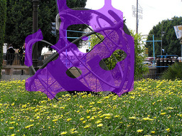
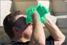
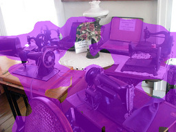
.5 .5 .5 .5 .5 .5 .5 .5 .5 .5 .5 .5 .5 .5 .5 .5

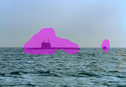
(b) C10

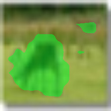
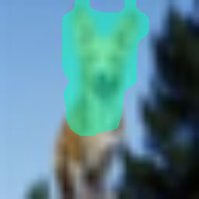
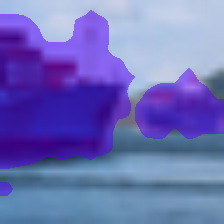
.5 .5 .5 .5 .5 .5 .5 .5 .5 .5 .5 .5 .5 .5 .5 .5

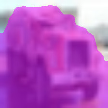
(c) C100

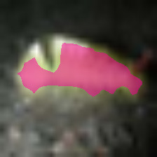
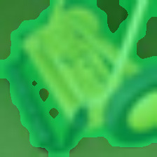
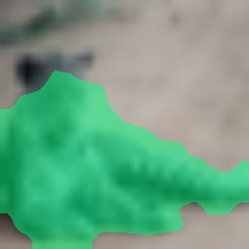
.5 .5 .5 .5 .5 .5 .5 .5 .5 .5 .5 .5 .5 .5 .5 .5

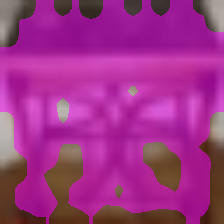
(d) CUB

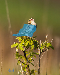
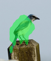
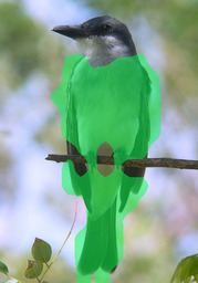
.5 .5 .5 .5 .5 .5 .5 .5 .5 .5 .5 .5 .5 .5 .5 .5

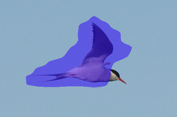
(e) Cars

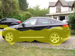
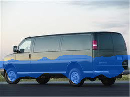
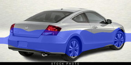
.5 .5 .5 .5 .5 .5 .5 .5 .5 .5 .5 .5 .5 .5 .5 .5

(f) Aircr

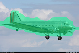
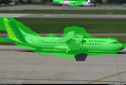
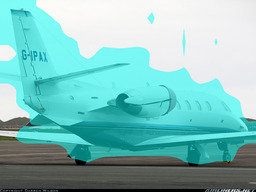
.5 .5 .5 .5 .5 .5 .5 .5 .5 .5 .5 .5 .5 .5 .5 .5

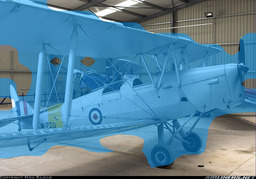
(g) Flowers

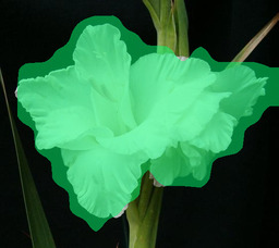
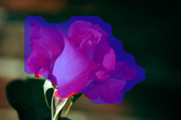
.5 .5 .5 .5 .5 .5 .5 .5 .5 .5 .5 .5 .5 .5 .5 .5

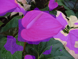
Figure 4: Informative image patches identified by ComFe using the DINOv2 ViT-S/14 backbone across randomly selected validation images from a range of datasets. Image patches classified as non-informative are left uncolored, while patches classified as a particular class are overlayed with a colored mask.

5.0.2 ComFe is able to localise salient image features across a range of datasets.

Fig. 4 shows that our approach learns to identify the image prototypes that relate to the classes of interest across a range of datasets, from small low resolution datasets with few classes like CIFAR-10, to large high resolution datasets with a thousand classes such as ImageNet. We observe that when identifying birds the head appears to be non-informative on the CUB200 dataset, and that the upper vehicle cabin and roof are non-informative in the Stanford Cars dataset. It is also noted that when multiple relevant objects appear (such as for the submarines, boats, planes and cars), these are also detected as informative.

(a) Aircr

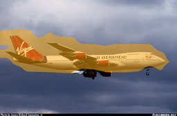
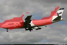
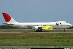
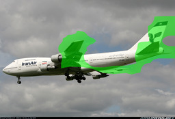
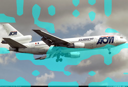
.5 .5 .5 .5 .5 .5 .5 .5 .5 .5 .5 .5 .5 .5 .5 .5 .5 .5 .5 .5 .5 .5 .5 .5 .5 .5 .5 .5

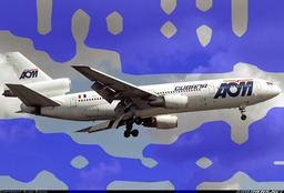
(b) Aircr

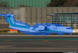
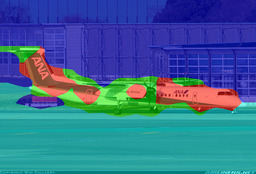
.5 .5 .5 .5 .5 .5 .5 .5 .5 .5 .5 .5 .5 .5 .5 .5 .5 .5 .5 .5 .5 .5 .5 .5 .5 .5 .5 .5

(c) Cars

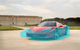
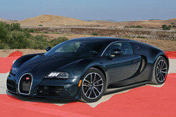
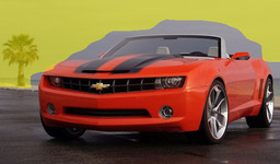
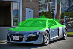
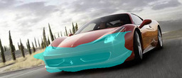
.5 .5 .5 .5 .5 .5 .5 .5 .5 .5 .5 .5 .5 .5 .5 .5 .5 .5 .5 .5 .5 .5 .5 .5 .5 .5 .5 .5

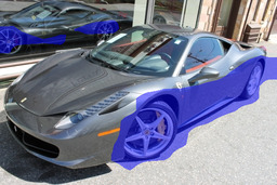
(d) Cars

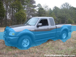
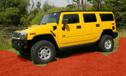
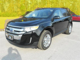
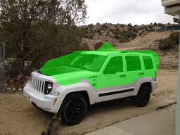
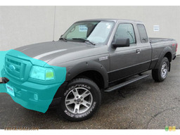
.5 .5 .5 .5 .5 .5 .5 .5 .5 .5 .5 .5 .5 .5 .5 .5 .5 .5 .5 .5 .5 .5 .5 .5 .5 .5 .5 .5

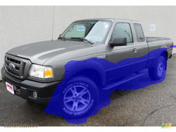
(e) CUB

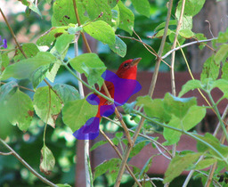
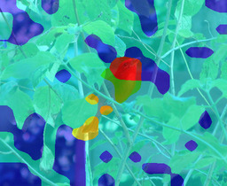
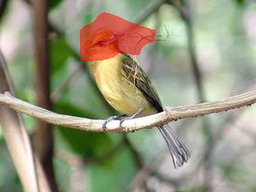
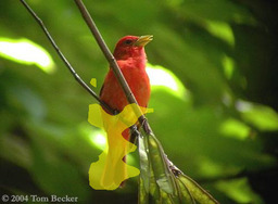
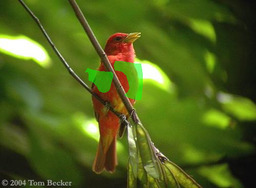
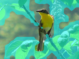
.5 .5 .5 .5 .5 .5 .5 .5 .5 .5 .5 .5 .5 .5 .5 .5 .5 .5 .5 .5 .5 .5 .5 .5 .5 .5 .5 .5

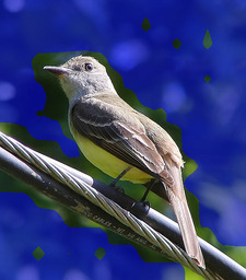
(f) CUB

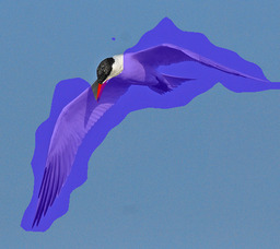
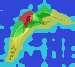
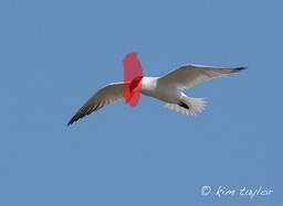
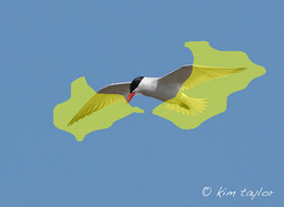
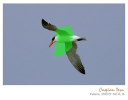
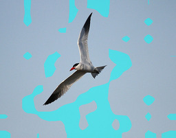
.5 .5 .5 .5 .5 .5 .5 .5 .5 .5 .5 .5 .5 .5 .5 .5 .5 .5 .5 .5 .5 .5 .5 .5 .5 .5 .5 .5

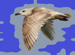
Figure 5: Example image prototype overlays and nearest neighbours on validation images from Pets, Cars and FGVC Aircraft obtained using ComFe with the DINOv2 ViT-S/14 backbone. The first row of images show the patches classified as a particular class (masked) or background (un-masked). The second row colors the patches according to which image prototype has highest probability given LABEL:eq:patch_probability. The other rows show the images from the training set that contained image prototypes with the largest cosine similarity to those in the second row.

5.0.3 The image prototypes learned by ComFe identify visual concepts.

In Fig. 5 it can be seen that the image prototypes partition images containing different classes in a consistent manner. On the FGVC Aircraft dataset, the first image prototype (red) identifies the cabin and body of the aircraft, while the second image prototype (yellow) identifies jet engines. There are only propellers on the first aircraft shown (Fig. 8(a)), so there are no patches associated with this image prototype that are highlighted for the second image (Fig. 8(d)). The third image prototype (green) identifies the wings and tail of the plane, and the final two image prototypes (blue and cyan) are always associated with the background and are classified as non-informative. Similar patterns are observed across the other datasets, with particular image prototypes identifying the front, side and upper cabin and roof of the car for Standford Cars, and the CUB200 dataset has image prototypes locating the head, body and wings and tail of each bird.

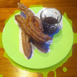
(a) Seed 1: 92.1%

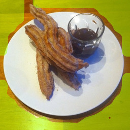
(b) Seed 2: 92.2%

(c) Seed 4: 92.3%

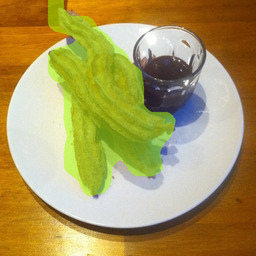
(d) Seed 3: 92.4%

Figure 6: Class predictions for patches using ComFe models initialised with different seeds for an image from the Food-101 validation set.

5.0.4 For some datasets and initialisations, ComFe transparently classifies using background features.

Like other clustering algorithms [1], ComFe is sensitive to the initialisation of the class prototypes. As shown in Fig. 6 for the Food-101 dataset, for particular initialisation seeds ComFe can find background features that can be used to accurately classify the training and validation data. However, there appears to be a trend accross both the Food-101 (Fig. 6) and Oxford Pets (Fig. S8) datasets that model initialisations resulting in salient image features being identified have better performance.

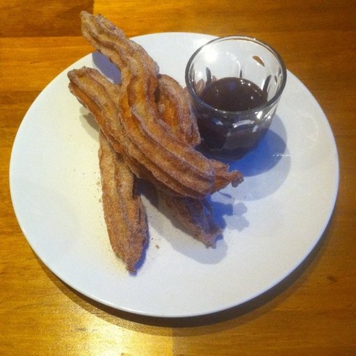
(a) Churros

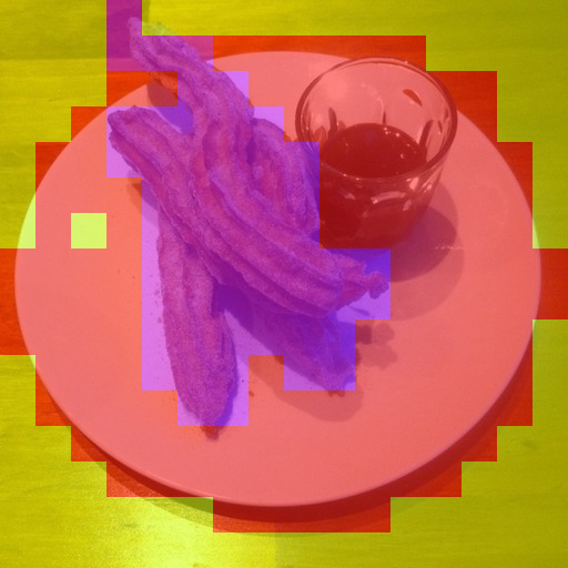
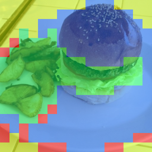
(b) Clustering with DINOv2

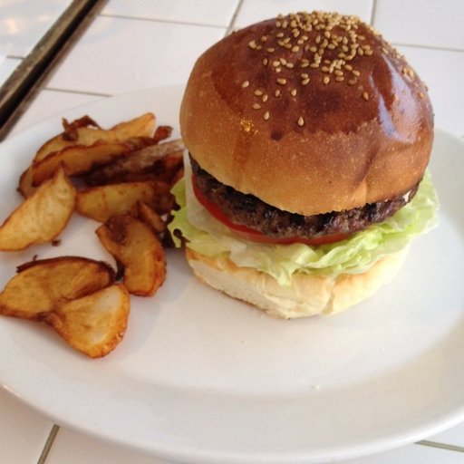
(c) Burger

Figure 7: Example image of churros and a burger on a white plate from the Food-101 validation set. The images in the middle are overlayed with a $k$-means clustering of the combined patch embeddings of the two images.

We observe that the DINOv2 patch embeddings are influenced by their context. For example, in Fig. 7 we use $k$-means clustering to visualise the DINOv2 patch embeddings of two images containing a white plate. We find that the surface the plates rest on both fall in the background cluster (yellow), but the plate containing churros is placed in the red cluster while the plate containing a burger is placed in the blue cluster. When ComFe obtains good performance in cases the salient parts of an image are classified as the background, this likely reflects this context leakage from the frozen backbone model.

Supplementary Material

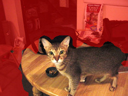
(a) Seed 1: 94.6%

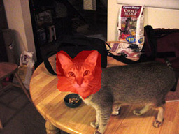
(b) Seed 4: 94.8%

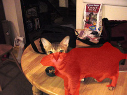
(c) Seed 3: 94.8%

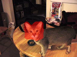
(d) Seed 2: 95.3%

Figure S8: Class predictions for patches using ComFe models initialised with different seeds for an image from the Oxford Pets validation set.

Table S5: Performance of ComFe with and without background class prototypes on ImageNet robustness and generalisation benchmarks. We report accuracy with a subset of the logits, restricted to only the classes present in the ImageNet-R [19] and ImageNet-A [20] test sets.

Backbone	Background	Test Dataset
	Prototypes	IN-R	IN-A
DINOv2 ViT-S/14 (f)	3000	57.7	42.6
DINOv2 ViT-B/14 (f)	3000	67.1	61.7
DINOv2 ViT-L/14 (f)	3000	72.5	71.9
DINOv2 ViT-L/14 (f)	0	73.8	75.2

Appendix 0.A Additional results

Table S6: Out-of-distribution (OOD) detection results for the ImageNet dataset on the OpenOOD benchmark [64] and other test sets using the DINOv2 ViT-S/14 backbone. All values are report as the AUROC of detecting the OOD data from the in-distribution data.

Methods	Datasets
	IN-V2	Sketch	IN-R	IN-A	IN-O	IN OpenOOD
						Near-OOD	Far-OOD
KNN+ [55]	55.3	81.0	79.2	83.5	80.8	72.6	92.7
Energy [30]	57.6	81.9	85.4	88.4	80.6	76.0	93.4
NN-Guide [44]	57.4	84.3	85.4	89.4	83.4	76.6	94.5
ComFe - $p_{\text{max}}(y,\textbf{P})$	57.8	81.6	81.8	84.6	81.4	80.2	90.4

0.A.0.1 ComFe can be used for out-of-distribution detection.

Our approach fits mixture model distributions to the data, allowing us to consider how well these might perform in detecting out-of-distribution (OOD) samples which may have lower likelihood. We find that the best approach combines the joint distribution over the image prototypes

$$p_{\text{max}}(y,\textbf{P})=\max_{y,i}p(y|\textbf{P}_{i})p(\textbf{P}_{i})$$ (30)

where the first term is defined by LABEL:eq:p_discrim and the second by summing out $y$ from LABEL:eq:gen_P_y. Tab. S6 compares this approach with other methods in the literature, using OOD datasets for ImageNet including ImageNet-O [20], OpenImage-O [60], SSB-hard [5], NINCO [58], iNaturalist [23] and Describable Textures [14] combined into Near-OOD and Far-OOD sets following the OpenOOD benchmark [64]. We find that while ComFe performs well for some datasets, specialised OOD approaches such as NN-Guide [44] perform better overall on the DINO-v2 embeddings.

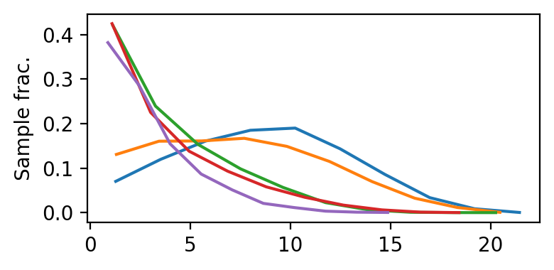
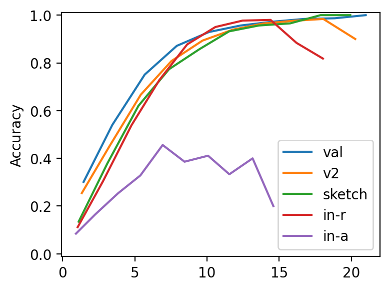
(a) Linear head with NN-Guide [44]

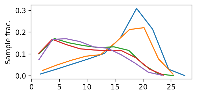
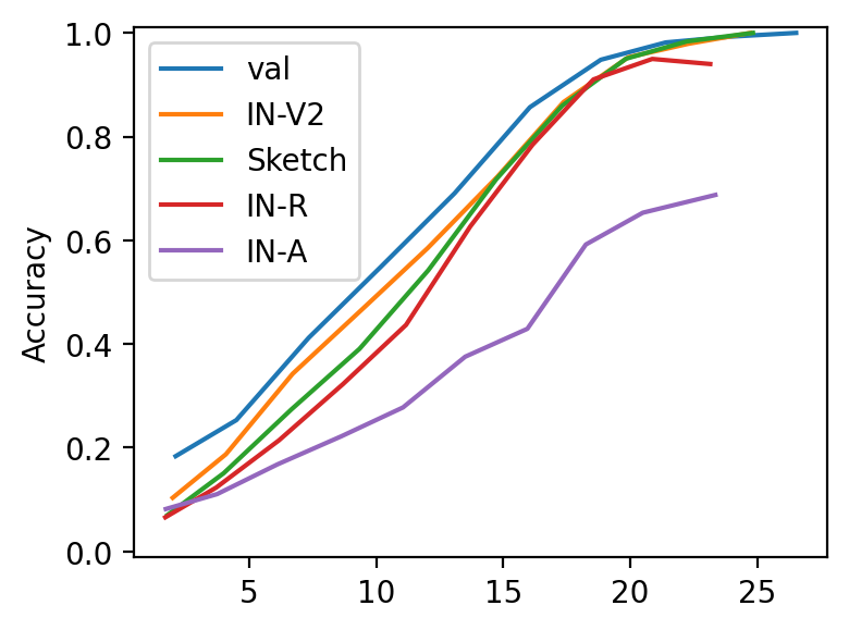
(b) ComFe - $p_{\text{max}}(y,\textbf{P})$

Figure S9: Reliability diagrams for different measures of model certainty using the ImageNet dataset and the DINOv2 ViT-S/14 backbone.

0.A.0.2 ComFe can detect images that are likely to have an unreliable prediction.

We consider the problem of identifying on a set of images that do not contain novel classes, whether the prediction is reliable. The OOD measure for ComFe $p_{\text{max}}(y,\textbf{P})$ combines confidence as well as support under the class prototype mixture model. An analogous measure could also be created with the NN-Guide OOD score, where we multiply it with the class confidence from a linear head. Reliability diagrams for both of these approaches are shown in Fig. S9, where it can be seen that the ComFe score correlates better with the observed accuracy.

Table S7: Performance of ComFe on the DINOv2 backbones with [43] and without [15] registers.

Backbone	Dataset
	IN-1K	C10	C100	Food	CUB	Pets	Cars	Aircr	Flowers
DINOv2 ViT-S/14 (f)	83.0	98.3	89.2	92.1	87.6	94.6	91.1	77.5	99.0
DINOv2 ViT-S/14 (f) w/reg	82.9	98.2	89.0	91.6	87.8	94.9	90.5	76.5	98.8
DINOv2 ViT-L/14 (f)	86.7	99.4	93.6	94.6	89.2	95.9	93.6	83.9	99.4
DINOv2 ViT-L/14 (f) w/reg	87.2	99.5	94.6	95.6	90.0	96.0	94.5	85.6	99.6

0.A.0.3 Including registers in the DINO-v2 ViT model can improve the performance of ComFe for large models.

Further work on the ViT backbone has found that including register tokens [15] can prevent embedding artefacts such as patch tokens with large norms, which improves results bigger models like ViT-L and the larger variants. In Tab. S7 we observe that for small models including registers results in poorer performance for ComFe, but that for the ViT-L model, performance is improved. We also find in Fig. S10 that for the ViT-L backbone without registers, for some classes a single patch can denote the class and the image prototypes can be less uniform. However, when registers are used the image prototypes are more descriptive and we were unable to find cases where salient features from the image were not identified.

(a) Class
          

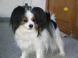
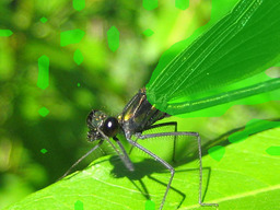
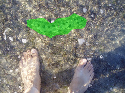
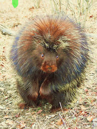
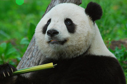
.5 .5 .5 .5 .5 .5 .5 .5 .5 .5 .5 .5 .5 .5 .5 .5 .5 .5 .5 .5 .5 .5 .5 .5

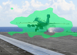
(b) Components
          

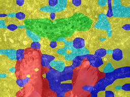
.5 .5 .5 .5 .5 .5 .5 .5 .5 .5 .5 .5 .5 .5 .5 .5 .5 .5 .5 .5 .5 .5 .5 .5

(c) Class
w/registers

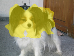
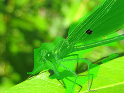
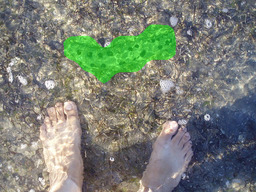
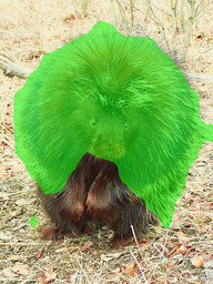
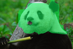
.5 .5 .5 .5 .5 .5 .5 .5 .5 .5 .5 .5 .5 .5 .5 .5 .5 .5 .5 .5 .5 .5 .5 .5

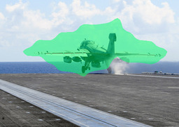
(d) Components
w/registers

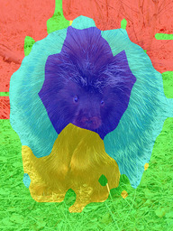
.5 .5 .5 .5 .5 .5 .5 .5 .5 .5 .5 .5 .5 .5 .5 .5 .5 .5 .5 .5 .5 .5 .5 .5

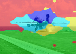
Figure S10: Components and patch classes from ComFe with the DINOv2 ViT-L/14 backbone trained on ImageNet. The left two columns are obtained using the ViT-L/14 backbone without registers, and the right two columns are obtained using the ViT-L/14 model that includes registers. Image patches classified as the background are left uncolored, while patches classified as a particular class are overlayed with a colored mask.

Appendix 0.B Ablation studies

Table S8: Performance of ComFe on the DINOv2 ViT-S/14 backbone with different numbers of transformer decoder layers. We report the mean and standard deviation of five runs. The bolded set of parameters is the default one used throughout this paper.

Transformer	Dataset
Layers	Aircr	Pets	Cars
1	75.9±1.0	94.9±0.2	90.2±0.2
2	76.0±0.8	94.6±0.5	91.0±0.4
4	77.1±1.3	94.5±0.3	91.1±0.4
6	77.6±1.2	94.6±0.5	91.2±0.4

Table S9: Performance of ComFe on the DINOv2 ViT-S/14 backbone with elements of the loss removed. In the loss term columns, an N denotes when a term is removed and a Y denotes when a term is kept. The bolded set of parameters is the default one used throughout this paper.

Loss term			Dataset
$p_{\text{max}}(y|\textbf{P})$	$L_{\text{CARL}}$	$L_{\text{contrast}}$	Aircr	Pets	Cars
N	Y	Y	74.8±1.5	94.8±0.5	90.1±0.8
Y	N	Y	75.8±0.8	94.6±0.5	91.0±0.2
Y	Y	N	76.2±0.6	94.6±0.6	90.7±0.3
Y	Y	Y	75.8±0.9	94.9±0.2	91.0±0.2

0.B.0.1 More transformer decoder layers improves performance for some datasets.

Tab. S8 shows that for the StanfordCars and the FGVC Aircraft datasets, including more transformer decoder layers improves the average performance of ComFe across a number of seeds. However, for the Oxford Pets dataset having a single transformer decoder layer leads to the best results.

0.B.0.2 Loss terms.

In Tab. S9 we explore the impact of removing loss terms on the performance of ComFe across the StanfordCars, FGVC Aircraft and Oxford Pets datasets. Removing the $p_{\text{max}}(y|\textbf{P})$ term from the discriminative loss leads to lower performance for the StanfordCars and FGVC Aircraft datasets, but has little impact on the performance on Oxford Pets. Adding or removing the other loss terms does not appear to have a significant impact on accuracy.

References

- [1] Al-Daoud, M.B., Roberts, S.A.: New methods for the initialisation of clusters. Pattern Recognition Letters 17(5), 451–455 (1996)
- [2] Assran, M., Caron, M., Misra, I., Bojanowski, P., Joulin, A., Ballas, N., Rabbat, M.: Semi-supervised learning of visual features by non-parametrically predicting view assignments with support samples. In: Proceedings of the IEEE/CVF International Conference on Computer Vision. pp. 8443–8452 (2021)
- [3] Bai, H., Ming, Y., Katz-Samuels, J., Li, Y.: Provable out-of-distribution generalization in hypersphere. In: The Twelfth International Conference on Learning Representations (2024), https://openreview.net/forum?id=VXak3CZZGC
- [4] Beloiu, M., Heinzmann, L., Rehush, N., Gessler, A., Griess, V.C.: Individual tree-crown detection and species identification in heterogeneous forests using aerial rgb imagery and deep learning. Remote Sensing 15(5), 1463 (2023)
- [5] Bitterwolf, J., Müller, M., Hein, M.: In or out? fixing imagenet out-of-distribution detection evaluation (2023)
- [6] Bossard, L., Guillaumin, M., Van Gool, L.: Food-101–mining discriminative components with random forests. In: Computer Vision–ECCV 2014: 13th European Conference, Zurich, Switzerland, September 6-12, 2014, Proceedings, Part VI 13. pp. 446–461. Springer (2014)
- [7] Carion, N., Massa, F., Synnaeve, G., Usunier, N., Kirillov, A., Zagoruyko, S.: End-to-end object detection with transformers. In: European conference on computer vision. pp. 213–229. Springer (2020)
- [8] Chen, C., Li, O., Tao, D., Barnett, A., Rudin, C., Su, J.K.: This looks like that: deep learning for interpretable image recognition. Advances in neural information processing systems 32 (2019)
- [9] Chen, T., Kornblith, S., Norouzi, M., Hinton, G.: A simple framework for contrastive learning of visual representations. In: International conference on machine learning. pp. 1597–1607. PMLR (2020)
- [10] Chen, T., Kornblith, S., Swersky, K., Norouzi, M., Hinton, G.E.: Big self-supervised models are strong semi-supervised learners. Advances in neural information processing systems 33, 22243–22255 (2020)
- [11] Chen, T., Luo, C., Li, L.: Intriguing properties of contrastive losses. Advances in Neural Information Processing Systems 34, 11834–11845 (2021)
- [12] Cheng, B., Misra, I., Schwing, A.G., Kirillov, A., Girdhar, R.: Masked-attention mask transformer for universal image segmentation. In: Proceedings of the IEEE/CVF conference on computer vision and pattern recognition. pp. 1290–1299 (2022)
- [13] Cherti, M., Beaumont, R., Wightman, R., Wortsman, M., Ilharco, G., Gordon, C., Schuhmann, C., Schmidt, L., Jitsev, J.: Reproducible scaling laws for contrastive language-image learning. In: Proceedings of the IEEE/CVF Conference on Computer Vision and Pattern Recognition. pp. 2818–2829 (2023)
- [14] Cimpoi, M., Maji, S., Kokkinos, I., Mohamed, S., Vedaldi, A.: Describing textures in the wild (2013)
- [15] Darcet, T., Oquab, M., Mairal, J., Bojanowski, P.: Vision transformers need registers. arXiv preprint arXiv:2309.16588 (2023)
- [16] Gotmare, A., Keskar, N.S., Xiong, C., Socher, R.: A closer look at deep learning heuristics: Learning rate restarts, warmup and distillation. arXiv preprint arXiv:1810.13243 (2018)
- [17] Grill, J.B., Strub, F., Altché, F., Tallec, C., Richemond, P., Buchatskaya, E., Doersch, C., Avila Pires, B., Guo, Z., Gheshlaghi Azar, M., et al.: Bootstrap your own latent-a new approach to self-supervised learning. Advances in neural information processing systems 33, 21271–21284 (2020)
- [18] He, K., Chen, X., Xie, S., Li, Y., Dollár, P., Girshick, R.: Masked autoencoders are scalable vision learners. In: Proceedings of the IEEE/CVF conference on computer vision and pattern recognition. pp. 16000–16009 (2022)
- [19] Hendrycks, D., Basart, S., Mu, N., Kadavath, S., Wang, F., Dorundo, E., Desai, R., Zhu, T., Parajuli, S., Guo, M., et al.: The many faces of robustness: A critical analysis of out-of-distribution generalization. In: Proceedings of the IEEE/CVF International Conference on Computer Vision. pp. 8340–8349 (2021)
- [20] Hendrycks, D., Zhao, K., Basart, S., Steinhardt, J., Song, D.: Natural adversarial examples. In: Proceedings of the IEEE/CVF Conference on Computer Vision and Pattern Recognition. pp. 15262–15271 (2021)
- [21] Hoffmann, A., Fanconi, C., Rade, R., Kohler, J.: This looks like that… does it? shortcomings of latent space prototype interpretability in deep networks. arXiv preprint arXiv:2105.02968 (2021)
- [22] Hong, Y., Wang, J., Sun, W., Pan, H.: Minimalist and high-performance semantic segmentation with plain vision transformers. arXiv preprint arXiv:2310.12755 (2023)
- [23] Horn, G.V., Aodha, O.M., Song, Y., Cui, Y., Sun, C., Shepard, A., Adam, H., Perona, P., Belongie, S.: The inaturalist species classification and detection dataset (2018)
- [24] Jiang, Z.H., Hou, Q., Yuan, L., Zhou, D., Shi, Y., Jin, X., Wang, A., Feng, J.: All tokens matter: Token labeling for training better vision transformers. Advances in neural information processing systems 34, 18590–18602 (2021)
- [25] Kim, S., Nam, J., Ko, B.C.: Vit-net: Interpretable vision transformers with neural tree decoder. In: International Conference on Machine Learning. pp. 11162–11172. PMLR (2022)
- [26] Kim, S.S., Meister, N., Ramaswamy, V.V., Fong, R., Russakovsky, O.: Hive: Evaluating the human interpretability of visual explanations. In: European Conference on Computer Vision. pp. 280–298. Springer (2022)
- [27] Krause, J., Stark, M., Deng, J., Fei-Fei, L.: 3d object representations for fine-grained categorization. In: Proceedings of the IEEE international conference on computer vision workshops. pp. 554–561 (2013)
- [28] Krizhevsky, A., Hinton, G., et al.: Learning multiple layers of features from tiny images (2009)
- [29] Lee, D.H., Liu, J.L.: End-to-end deep learning of lane detection and path prediction for real-time autonomous driving. Signal, Image and Video Processing 17(1), 199–205 (2023)
- [30] Liu, W., Wang, X., Owens, J., Li, Y.: Energy-based out-of-distribution detection. Advances in neural information processing systems 33, 21464–21475 (2020)
- [31] Loshchilov, I., Hutter, F.: Sgdr: Stochastic gradient descent with warm restarts. arXiv preprint arXiv:1608.03983 (2016)
- [32] Loshchilov, I., Hutter, F.: Decoupled weight decay regularization. arXiv preprint arXiv:1711.05101 (2017)
- [33] Lu, H., Gong, D., Wang, S., Xue, J., Yao, L., Moore, K.: Learning with mixture of prototypes for out-of-distribution detection. In: The Twelfth International Conference on Learning Representations (2024), https://openreview.net/forum?id=uNkKaD3MCs
- [34] Maji, S., Rahtu, E., Kannala, J., Blaschko, M., Vedaldi, A.: Fine-grained visual classification of aircraft. arXiv preprint arXiv:1306.5151 (2013)
- [35] Mannix, E., Bondell, H.: Efficient out-of-distribution detection with prototypical semi-supervised learning and foundation models. arXiv preprint (2023)
- [36] Marin, J.M., Mengersen, K., Robert, C.P.: Bayesian modelling and inference on mixtures of distributions. Handbook of statistics 25, 459–507 (2005)
- [37] Mikolov, T., et al.: Statistical language models based on neural networks. Presentation at Google, Mountain View, 2nd April 80(26) (2012)
- [38] Ming, Y., Sun, Y., Dia, O., Li, Y.: How to exploit hyperspherical embeddings for out-of-distribution detection? arXiv preprint arXiv:2203.04450 (2022)
- [39] Mo, S., Su, J.C., Ma, C.Y., Assran, M., Misra, I., Yu, L., Bell, S.: Ropaws: Robust semi-supervised representation learning from uncurated data. arXiv preprint arXiv:2302.14483 (2023)
- [40] Nauta, M., Schlötterer, J., van Keulen, M., Seifert, C.: Pip-net: Patch-based intuitive prototypes for interpretable image classification. In: Proceedings of the IEEE/CVF Conference on Computer Vision and Pattern Recognition. pp. 2744–2753 (2023)
- [41] Nauta, M., Van Bree, R., Seifert, C.: Neural prototype trees for interpretable fine-grained image recognition. In: Proceedings of the IEEE/CVF Conference on Computer Vision and Pattern Recognition. pp. 14933–14943 (2021)
- [42] Nilsback, M.E., Zisserman, A.: Automated flower classification over a large number of classes. In: 2008 Sixth Indian conference on computer vision, graphics & image processing. pp. 722–729. IEEE (2008)
- [43] Oquab, M., Darcet, T., Moutakanni, T., Vo, H., Szafraniec, M., Khalidov, V., Fernandez, P., Haziza, D., Massa, F., El-Nouby, A., et al.: Dinov2: Learning robust visual features without supervision. arXiv preprint arXiv:2304.07193 (2023)
- [44] Park, J., Jung, Y.G., Teoh, A.B.J.: Nearest neighbor guidance for out-of-distribution detection. In: Proceedings of the IEEE/CVF International Conference on Computer Vision. pp. 1686–1695 (2023)
- [45] Parkhi, O.M., Vedaldi, A., Zisserman, A., Jawahar, C.: Cats and dogs. In: 2012 IEEE conference on computer vision and pattern recognition. pp. 3498–3505. IEEE (2012)
- [46] Paul, D., Chowdhury, A., Xiong, X., Chang, F.J., Carlyn, D., Stevens, S., Provost, K., Karpatne, A., Carstens, B., Rubenstein, D., et al.: A simple interpretable transformer for fine-grained image classification and analysis. arXiv preprint arXiv:2311.04157 (2023)
- [47] Radford, A., Kim, J.W., Hallacy, C., Ramesh, A., Goh, G., Agarwal, S., Sastry, G., Askell, A., Mishkin, P., Clark, J., et al.: Learning transferable visual models from natural language supervision. In: International conference on machine learning. pp. 8748–8763. PMLR (2021)
- [48] Recht, B., Roelofs, R., Schmidt, L., Shankar, V.: Do imagenet classifiers generalize to imagenet? In: International conference on machine learning. pp. 5389–5400. PMLR (2019)
- [49] Rudin, C.: Stop explaining black box machine learning models for high stakes decisions and use interpretable models instead. Nature machine intelligence 1(5), 206–215 (2019)
- [50] Russakovsky, O., Deng, J., Su, H., Krause, J., Satheesh, S., Ma, S., Huang, Z., Karpathy, A., Khosla, A., Bernstein, M., Berg, A.C., Fei-Fei, L.: ImageNet Large Scale Visual Recognition Challenge. International Journal of Computer Vision (IJCV) 115(3), 211–252 (2015). https://doi.org/10.1007/s11263-015-0816-y
- [51] Rymarczyk, D., Struski, Ł., Górszczak, M., Lewandowska, K., Tabor, J., Zieliński, B.: Interpretable image classification with differentiable prototypes assignment. In: European Conference on Computer Vision. pp. 351–368. Springer (2022)
- [52] Rymarczyk, D., Struski, Ł., Tabor, J., Zieliński, B.: Protopshare: Prototypical parts sharing for similarity discovery in interpretable image classification. In: Proceedings of the 27th ACM SIGKDD Conference on Knowledge Discovery & Data Mining. pp. 1420–1430 (2021)
- [53] Silva, T., Rivera, A.R.: Representation learning via consistent assignment of views to clusters. In: Proceedings of the 37th ACM/SIGAPP Symposium on Applied Computing. pp. 987–994 (2022)
- [54] Snell, J., Swersky, K., Zemel, R.: Prototypical networks for few-shot learning. Advances in neural information processing systems 30 (2017)
- [55] Sun, Y., Ming, Y., Zhu, X., Li, Y.: Out-of-distribution detection with deep nearest neighbors. In: International Conference on Machine Learning. pp. 20827–20840. PMLR (2022)
- [56] Tukra, S., Hoffman, F., Chatfield, K.: Improving visual representation learning through perceptual understanding. In: Proceedings of the IEEE/CVF Conference on Computer Vision and Pattern Recognition. pp. 14486–14495 (2023)
- [57] Vaswani, A., Shazeer, N., Parmar, N., Uszkoreit, J., Jones, L., Gomez, A.N., Kaiser, Ł., Polosukhin, I.: Attention is all you need. Advances in neural information processing systems 30 (2017)
- [58] Vaze, S., Han, K., Vedaldi, A., Zisserman, A.: Open-set recognition: A good closed-set classifier is all you need. In: International Conference on Learning Representations (2022), https://openreview.net/forum?id=5hLP5JY9S2d
- [59] Wang, H., Ge, S., Lipton, Z., Xing, E.P.: Learning robust global representations by penalizing local predictive power. Advances in Neural Information Processing Systems 32 (2019)
- [60] Wang, H., Li, Z., Feng, L., Zhang, W.: Vim: Out-of-distribution with virtual-logit matching. In: Proceedings of the IEEE/CVF Conference on Computer Vision and Pattern Recognition (CVPR). pp. 4921–4930 (June 2022)
- [61] Welinder, P., Branson, S., Mita, T., Wah, C., Schroff, F., Belongie, S., Perona, P.: Caltech-ucsd birds 200 (2010)
- [62] Xue, M., Huang, Q., Zhang, H., Cheng, L., Song, J., Wu, M., Song, M.: Protopformer: Concentrating on prototypical parts in vision transformers for interpretable image recognition. arXiv preprint arXiv:2208.10431 (2022)
- [63] Yang, H.M., Zhang, X.Y., Yin, F., Liu, C.L.: Robust classification with convolutional prototype learning. In: Proceedings of the IEEE conference on computer vision and pattern recognition. pp. 3474–3482 (2018)
- [64] Yang, J., Wang, P., Zou, D., Zhou, Z., Ding, K., Peng, W., Wang, H., Chen, G., Li, B., Sun, Y., et al.: Openood: Benchmarking generalized out-of-distribution detection. Advances in Neural Information Processing Systems 35, 32598–32611 (2022)
- [65] Yang, Y.Y., Chou, C.N., Chaudhuri, K.: Understanding rare spurious correlations in neural networks. In: ICML 2022: Workshop on Spurious Correlations, Invariance and Stability (2022), https://openreview.net/forum?id=iHU9Ze_5X7n
- [66] Zhao, B., Yu, Z., Lan, S., Cheng, Y., Anandkumar, A., Lao, Y., Alvarez, J.M.: Fully attentional networks with self-emerging token labeling. In: Proceedings of the IEEE/CVF International Conference on Computer Vision. pp. 5585–5595 (2023)
- [67] Zhou, B., Khosla, A., Lapedriza, A., Oliva, A., Torralba, A.: Learning deep features for discriminative localization. In: Proceedings of the IEEE conference on computer vision and pattern recognition. pp. 2921–2929 (2016)
- [68] Zhou, S.K., Greenspan, H., Shen, D.: Deep learning for medical image analysis. Academic Press (2023)
- [69] Zhou, S., Bondell, H., Tordesillas, A., Rubinstein, B.I.P., Bailey, J.: Early identification of an impending rockslide location via a spatially-aided Gaussian mixture model. The Annals of Applied Statistics 14(2), 977 – 992 (2020). https://doi.org/10.1214/20-AOAS1326, https://doi.org/10.1214/20-AOAS1326