Helmholtz preconditioning for the compressible Euler equations using mixed finite elements with Lorenz staggering

Abstract

Implicit solvers for atmospheric models are often accelerated via the solution of a preconditioned system. For block preconditioners this typically involves the factorisation of the (approximate) Jacobian for the coupled system into a Helmholtz equation for some function of the pressure. Here we present a preconditioner for the compressible Euler equations with a flux form representation of the potential temperature on the Lorenz grid using mixed finite elements. This formulation allows for spatial discretisations that conserve both energy and potential temperature variance. By introducing the dry thermodynamic entropy as an auxiliary variable for the solution of the algebraic system, the resulting preconditioner is shown to have a similar block structure to an existing preconditioner for the material form transport of potential temperature on the Charney-Phillips grid, and to be more efficient and stable than either this or a previous Helmholtz preconditioner for the flux form transport of density weighted potential temperature on the Lorenz grid for a one dimensional thermal bubble configuration. The new preconditioner is further verified against standard two dimensional test cases in a vertical slice geometry.

1 Introduction

Models of compressible atmospheric dynamics must be stable for processes across a range of temporal scales, including fast acoustic and inertio-gravity waves as well as sub-critical inertial motions. In order to ensure stability over long time steps that do not explicitly resolve fast processes, models often use implicit time stepping methods. The solution of the resulting algebraic system is often preconditioned via the approximate block factorisation of the Jacobian operator for the coupled system into a single Helmholtz equation for some form of the pressure. This may be applied as part of a fully implicit three dimensional solver [1, 2, 3, 4], or as part of a horizontally explicit-vertically implicit dimensional splitting [5, 6, 7]. If the velocity space is hybridized such that the continuity of winds across cell boundaries is enforced via an additional set of Lagrange multipliers rather than the unique solution of the wind at the boundaries, then the Helmholtz equation may alternatively be expressed in terms of these Lagrange multipliers instead of the pressure variable [8, 9].

The Jacobian matrix from which the Helmholtz operator is derived is typically approximated so as to account for the stiff terms associated with fast time scales, while omitting or linearising those associated with other processes. This is due to the computational expense of assembling the full Jacobian, and also in the case of mixed finite element methods because the resulting Helmholtz operator is only semi-definite due to the approximate lumping of mass matrix inverses during block factorisation and so cannot be reliably solved to convergence.

There are numerous choices as to how the approximations to the Jacobian and the resulting Helmholtz operator are formulated, in addition to the choices one may make in terms of equation form and spatial discretisation. This article compares several different formulations of the Helmholtz operator for a dry compressible atmosphere, that result from different vertical placements of the potential temperature (the Lorenz and Charney-Phillips grids [10, 11]) and different forms of the potential temperature transport equation (flux form and material form) within mixed finite element spatial discretisations [3, 12, 5],

There are different benefits and drawbacks to these different modelling choices. With regards to the choice of function space for the thermodynamic variable, collocating this with the vertical velocity ensures that there are no spurious computational modes, as is the case when this is collocated with the pressure [10], and also provides for an optimal representation of buoyancy modes [11, 13]. However, while collocating the thermodynamic variable with the pressure variable on discontinuous spaces within elements does admit a spurious buoyancy mode, it also allows for energy conserving discretisations, [14, 5, 6] since the variational derivative of the thermodynamic variable is a function of the pressure, and so collocating these ensures that the chain rule required for the balance of kinetic and internal energy exchanges may be discretely preserved.

If the density and the thermodynamic variable are staggered, then the transport equations for these variables are not consistent if the thermodynamic variable is represented as a density weighted quantity in flux form [15]. However, if they are collocated, then a material form transport equation for the thermodynamic variable may be consistently derived from its density weighted flux form equivalent. Consequently we are free to choose between flux form and material form representations of the thermodynamic variable if this is collocated with the density. Using flux form transport of the thermodynamic variable allows for the conservation of its quadratic variance, and since this is a mathematical entropy of the dry compressible Euler equations, doing so can improve model stability [16].

In the present article we compare four choices of mixed finite element formulations of the compressible Euler equations from those referenced above, in terms of the stability and convergence of the Helmholtz operators implied by their discretisation. These include Helmholtz operators for the material transport of potential temperature, collocated with the vertical velocity (the Charney-Phillips grid) [3]; the flux form transport of density weighted potential temperature collocated with the Exner pressure (the Lorenz grid) [5]; the material transport of potential temperature on the Lorenz grid; and a novel alternative formulation of the flux form potential temperature on the Lorenz grid where this is re-scaled to derive a material form transport equation for the thermodynamic entropy, leading to a block structure and temporal scalings that more closely match those for material transport on the Charney-Phillips grid.

The remainder of this article is structured as follows. In Section 2 the mixed finite element discretisation of the compressible Euler equations will be introduced. For a more detailed discussion of this subject the reader is directed to the references therein. Section 3 details the formulation of a novel Helmholtz preconditioner for the flux form representation of the density weighted potential temperature on the Lorenz grid, and compares this to previous Helmholtz operator formulations. Results comparing these three formulations are presented in Section  4, including both detailed comparisons in 1D, and reproductions of standard test cases for the new preconditioner in 2D. Finally, conclusions and future research directions will be discussed in Section 5.

2 Mixed finite element discretisation of the compressible Euler equations

The compressible Euler equations for atmospheric motion may be described in terms of the velocity, $\boldsymbol{u}$, density, $\rho$, density weighted potential temperature, $\Theta$, and the Exner pressure, $\Pi$ as

$$\frac{\partial\boldsymbol{u}}{\partial t}+\boldsymbol{q}\times\boldsymbol{F}+\nabla\Phi+\theta\nabla\Pi =0$$ (1a)

$$\frac{\partial\rho}{\partial t}+\nabla\cdot\boldsymbol{F} =0$$ (1b)

$$\frac{\partial\Theta}{\partial t}+\nabla\cdot(\theta\boldsymbol{F}) =0$$ (1c)

$$\Pi-c_{p}\Big{(}\frac{R\Theta}{p_{0}}\Big{)}^{R/c_{v}} =0\ ,$$ (1d)

where $p_{0}$ is the reference pressure, $R=c_{p}-c_{v}$ is the ideal gas constant, $\boldsymbol{F}=\rho\boldsymbol{u}$ is the momentum, $\Phi=\frac{1}{2}\boldsymbol{u}\cdot\boldsymbol{u}+gz\hat{\boldsymbol{k}}$ is the Bernoulli potential, $\theta=\Theta/\rho$ is the potential temperature and

$$\boldsymbol{q}=\frac{\nabla\times\boldsymbol{u}+f\hat{\boldsymbol{k}}}{\rho}\ ,$$ (2)

is the potential vorticity, $f$ is the Coriolis term, $g$ is the gravitational constant and $\hat{\boldsymbol{k}}$ is the unit vector radially pointing outwards.

This system of partial differential equations may be spatially discretised using a mixed finite element method [17, 3, 5]. To this end, we first introduce the discrete subspaces over the three dimensional domain $\Omega$ as $\mathbb{W}_{0}\subset H_{1}(\Omega)$, $\mathbb{W}_{1}\subset H(\mathrm{curl},\Omega)$, $\mathbb{W}_{2}\subset H(\mathrm{div},\Omega)$, $\mathbb{W}_{3}\subset L^{2}(\Omega)$. The Lorenz staggering of the solution variables may be achieved for the mixed finite element form of the discrete problem by assigning the discrete solution variables (denoted by the subscript $h$) to the finite element spaces as $\boldsymbol{u}_{h}\in\mathbb{W}_{2}$, $\rho_{h},\Theta_{h},\Pi_{h}\in\mathbb{W}_{3}$. Additionally, we may assign the diagnostic fields as $\boldsymbol{q}_{h}\in\mathbb{W}_{1}$, $\boldsymbol{F}_{h}\in\mathbb{W}_{2}$, $\Phi_{h},\theta_{h}\in\mathbb{W}_{3}$.

The discrete variational form of the system is then derived by multiplying the equations in (1) by the test functions $\boldsymbol{v}_{h}\in\mathbb{W}_{2}$, $\phi_{h},\psi_{h},\chi_{h}\in\mathbb{W}_{3}$, respectively, and integrating over the domain $\Omega$ for a time step of $\Delta t$ between time level $n$ and the new time level at nonlinear iteration $k$ as

$$\int\boldsymbol{v}_{h}\cdot\frac{(\boldsymbol{u_{h}}^{k}-\boldsymbol{u}_{h}^{n})}{\Delta t}+\boldsymbol{v}_{h}\cdot\overline{\boldsymbol{q}}_{h}\times\overline{\boldsymbol{F}}_{h}-(\nabla\cdot\boldsymbol{v}_{h})\overline{\Phi}_{h}-\nabla\cdot(\boldsymbol{v}_{h}\overline{\theta}_{h})\overline{\Pi}_{h}\mathrm{d}\Omega+\int[\![\overline{\theta}_{h}\boldsymbol{v}_{h}\cdot\hat{\boldsymbol{n}}_{\Gamma}]\!]\{\mskip-5.0mu\{\overline{\Pi}_{h}\}\mskip-5.0mu\}\mathrm{d}\Gamma$$ (3a)

$$-\int c[\![\overline{\theta}_{h}\boldsymbol{v}_{h}\cdot\hat{\boldsymbol{n}}_{\Gamma}]\!][\![\overline{\Pi}_{h}]\!]\mathrm{d}\Gamma =\mathcal{R}_{u}$$

$$\int\phi_{h}\frac{(\rho_{h}^{k}-\rho_{h}^{n})}{\Delta t}+\phi_{h}\nabla\cdot\overline{\boldsymbol{F}}_{h}\mathrm{d}\Omega =\mathcal{R}_{\rho}$$ (3b)

$$\int\psi_{h}\frac{(\Theta_{h}^{k}-\Theta_{h}^{n})}{\Delta t}+\psi_{h}\nabla\cdot(\overline{\theta}_{h}\overline{\boldsymbol{F}})_{h}\mathrm{d}\Omega-\int[\![\overline{\theta}_{h}\overline{\boldsymbol{F}}_{h}\cdot\hat{\boldsymbol{n}}_{\Gamma}]\!]\{\mskip-5.0mu\{\psi_{h}\}\mskip-5.0mu\}\mathrm{d}\Gamma+\int c[\![\overline{\theta}_{h}\overline{\boldsymbol{F}}_{h}\cdot\hat{\boldsymbol{n}}_{\Gamma}]\!][\![\psi_{h}]\!]\mathrm{d}\Gamma =\mathcal{R}_{\Theta}$$ (3c)

$$\int\chi_{h}\log(\Pi_{h}^{k})-\chi_{h}\frac{R}{c_{v}}\log(\Theta_{h}^{k})-\chi_{h}\frac{R}{c_{v}}\log\Big{(}\frac{R}{p_{0}}\Big{)}-\chi_{h}\log(c_{p})\mathrm{d}\Omega =\mathcal{R}_{\Pi}\ ,$$ (3d)

where $\mathcal{R}_{u}$, $\mathcal{R}_{\rho}$, $\mathcal{R}_{\Theta}$, $\mathcal{R}_{\Pi}$ are the different components of the discrete nonlinear residual functional, and $c=sign(\overline{\boldsymbol{F}}_{h}\cdot\hat{\boldsymbol{n}}_{\Gamma})/2$ in (3c) indicates an upwinded density weighted potential temperature flux, as well as its energy conserving adjoint in (3a), and $c=0$ indicates a centered flux. Note that in (3d) we have taken the natural logarithm of the original equation of state (1d). Note also that integration by parts has been selectively applied where the trial space does not support the necessary differential operator. We have also included internal boundary integrals over the element faces, $\Gamma$, for which the unit normal vector is defined as $\hat{\boldsymbol{n}}_{\Gamma}$, involving both jumps, $[\![a_{h}]\!]:=a_{h}^{+}-a_{h}^{-}$ and means, $\{\mskip-5.0mu\{a\}\mskip-5.0mu\}:=(a_{h}^{+}+a_{h}^{-})/2$, where $a_{h}^{+}$ and $a_{h}^{-}$ refer to the evaluation of a discrete quantity $a_{h}$ from the elements on the right and left side of the face respectively. The overbar $\overline{a}_{h}$ denotes exact second order time integration of $a_{h}$. For linear quantities this is nothing more than a simple averaging. The exception to this are the quadratic nonlinear terms $\overline{\boldsymbol{F}}_{h}$ and $\overline{\Phi}_{h}$, for which this is computed using Simpson’s rule. Doing so ensures that these are exactly integrated in time for a second order temporal integration, which is necessary for exact temporal conservation of energy [18, 15, 5], which is given as

$$\mathcal{H}_{h}=\int\frac{\rho_{h}\boldsymbol{u}_{h}\cdot\boldsymbol{u}_{h}}{2}+\rho_{h}gz+\frac{c_{v}}{c_{p}}\Theta_{h}\Pi_{h}\mathrm{d}\Omega\ .$$ (4)

The diagnostic equations are spatially discretised in a similar manner by introducing test functions $\boldsymbol{\omega}_{h}\in\mathbb{W}_{1}$, $\boldsymbol{w}_{h}\in\mathbb{W}_{2}$, $\xi_{h},\sigma_{h}\in\mathbb{W}_{3}$ as

$$\int\overline{\rho}_{h}\boldsymbol{\omega}_{h}\cdot\overline{\boldsymbol{q}}_{h}\mathrm{d}\Omega= \int-(\nabla\times\boldsymbol{\omega}_{h})\cdot\overline{\boldsymbol{u}}_{h}+\ \boldsymbol{\omega}_{h}\cdot f\hat{\boldsymbol{k}}\mathrm{d}\Omega$$ (5a)

$$\int\boldsymbol{w}_{h}\cdot\overline{\boldsymbol{F}}_{h}\mathrm{d}\Omega= \int\frac{\boldsymbol{w}_{h}}{6}\cdot(2\rho_{h}^{n}\boldsymbol{u}_{h}^{n}+\rho_{h}^{n}\boldsymbol{u}_{h}^{k}+\rho_{h}^{k}\boldsymbol{u}_{h}^{n}+2\rho_{h}^{k}\boldsymbol{u}_{h}^{k})\mathrm{d}\Omega$$ (5b)

$$\int\xi_{h}\overline{\Phi}_{h}\mathrm{d}\Omega= \int\frac{1}{6}\xi_{h}\Big{(}\boldsymbol{u}_{h}^{n}\cdot\boldsymbol{u}_{h}^{n}+\boldsymbol{u}_{h}^{n}\cdot\boldsymbol{u}_{h}^{k}+\boldsymbol{u}_{h}^{k}\cdot\boldsymbol{u}_{h}^{k}\Big{)}+\xi_{h}gz\hat{\boldsymbol{k}}\mathrm{d}\Omega$$ (5c)

$$\int\sigma_{h}\overline{\rho}_{h}\overline{\theta}_{h}\mathrm{d}\Omega= \int\sigma_{h}\overline{\Theta}_{h}\mathrm{d}\Omega\ .$$ (5d)

Note that the discretisation presented in (3) is generalised to a three dimensional domain. However the examples presented below are all for one or two dimensional domains. For the one dimensional domain, we have that $\overline{\boldsymbol{q}}_{h}:=0$ in (3a), such that (5a) is unnecessary. For the two dimensional case we have that the potential vorticity is effectively a scalar function, $\overline{q}_{h}\in\mathbb{W}_{0}$, which is diagnosed subject to the test function $\omega_{h}\in\mathbb{W}_{0}$ in (5a). In all cases presented here there is also no Coriolis term, such that $f:=0$.

2.1 Damping in multiple dimensions

In order to suppress grid scale oscillations for the two dimensional test cases described below we also introduce a continuous interior penalty term [19], which penalises against jumps in the mass flux gradient at element boundaries, and is added to the discrete momentum equation (3a) as

$$\int\Delta x^{2}u_{m}\{\mskip-5.0mu\{\overline{\alpha}_{h}\}\mskip-5.0mu\}[\![\nabla\boldsymbol{v}_{h}\cdot\hat{\boldsymbol{n}}_{\Gamma}]\!][\![\nabla\overline{\boldsymbol{F}}_{h}\cdot\hat{\boldsymbol{n}}_{\Gamma}]\!]\mathrm{d}\Gamma\qquad\forall\boldsymbol{v}_{h}\in\mathbb{W}_{2}\ ,$$ (6)

where $\Delta x$ is the element spacing, $u_{m}=0.5$ is damping parameter that scales with the mean velocity, and $\overline{\alpha}_{h}$ is the discrete inverse density averaged over the time level, computed within each element as

$$\int\phi_{h}\overline{\rho}_{h}\overline{\alpha}_{h}\mathrm{d}\Omega=\int\phi_{h}\mathrm{d}\Omega\qquad\forall\phi_{h}\in\mathbb{W}_{3}.$$ (7)

A linearised form of this term is also added to the Helmholtz operator, via a correction to (15c) as

$$\Delta t\int\Delta x^{2}u_{m}[\![\nabla\boldsymbol{v}_{h}\cdot\hat{\boldsymbol{n}}_{\Gamma}]\!][\![\nabla\boldsymbol{w}_{h}\cdot\hat{\boldsymbol{n}}_{\Gamma}]\!]\mathrm{d}\Gamma\qquad\forall\boldsymbol{v}_{h},\boldsymbol{w}_{h}\in\mathbb{W}_{2}\ .$$ (8)

The variational derivatives of the discrete energy with respect to the prognostic variables are given by (5b), (5c) and (3d) respectively. Setting the test functions for the prognostic equations (3a), (3b), (3c) from these as $\overline{\boldsymbol{F}}_{h}$, $\overline{\Phi}_{h}$ and $\overline{\Pi}_{h}$ respectively leads to the cancellation of all forcing terms, with the exception of the continuous interior penalty term, and the evolution of total energy (4) as

$$\frac{\mathrm{d}\mathcal{H}_{h}}{\mathrm{d}t}=\int\overline{\boldsymbol{F}}_{h}\cdot\frac{\partial\boldsymbol{u}_{h}}{\partial t}+\overline{\Phi}_{h}\frac{\partial\rho_{h}}{\partial t}+\overline{\Pi}_{h}\frac{\partial\Theta_{h}}{\partial t}\mathrm{d}\Omega=-\int\Delta x^{2}u_{m}\{\mskip-5.0mu\{\overline{\alpha}_{h}\}\mskip-5.0mu\}([\![\nabla\overline{\boldsymbol{F}}_{h}\cdot\hat{\boldsymbol{n}}_{\Gamma}]\!])^{2}\mathrm{d}\Gamma\ .$$ (9)

Assuming $\overline{\rho}_{h},\overline{\alpha}_{h}>0$ and $u_{m}\geq 0$, setting $\boldsymbol{v}_{h}=\overline{\boldsymbol{F}}_{h}$ in (3a) and (6) results in a term that is always energy neutral or damping.

In addition to the interior penalty term (6), we also upwind the potential vorticity using the anticipated potential vorticity method (APVM) [20], in order to suppress the onset of grid scale noise associated with rotational motions. The application of the APVM involves replacing the scalar two dimensional potential vorticity $\overline{q}_{h}$ in (3a) with its upwinded variant $\overline{q}_{h}-\tau\overline{\boldsymbol{u}}_{h}\cdot\nabla\overline{q}_{h}$, where we use here as the upwinding factor $\tau=0.1\Delta t$, which is smaller than the typical value of $0.5\Delta t$ owing to the long time steps of our implicit solver. Since the APVM does not alter the antisymmetry of the coupled system (3), it does not break energy conservation.

As for the 1D tests, no upwinding is applied such that $c=0$ in both (3a) and (3c). However we note that since this term is applied in a skew symmetric way in these two equations, the presence of upwinding would not change the energy conservation result presented above.

In addition to the bottom and top boundary conditions described in the previous section, the two dimensional test cases described below also apply a periodic boundary condition in the horizontal dimension. Since it is not practical to directly compute matrix inverses for larger problem sizes in parallel, the two dimensional configurations use the lumped inverse formulation with four nonlinear iterations per time step.

3 Helmholtz preconditioning

In order to introduce the block preconditioner used in this work, we first recall that in the continuous form the thermodynamic entropy, $c_{p}\log(\theta)$ is subject to a material form advection equation [6], and that this may be derived from the density and density weighted potential temperature flux form transport equations. Scaling (1b) and (1c) respectively by $\rho^{-1}$ and $\Theta^{-1}$ and taking the difference of these gives

$$\frac{1}{\Theta}\Big{(}\frac{\partial\Theta}{\partial t}+\nabla\cdot(\theta\boldsymbol{F})\Big{)}-\frac{1}{\rho}\Big{(}\frac{\partial\rho}{\partial t}+\nabla\cdot\boldsymbol{F}\Big{)} =\frac{1}{\Theta}\frac{\partial\Theta}{\partial t}-\frac{1}{\rho}\frac{\partial\rho}{\partial t}+\frac{\boldsymbol{u}}{\theta}\cdot\nabla\theta$$ (10a)

$$=\frac{\partial}{\partial t}\log\Big{(}\frac{\Theta}{\rho}\Big{)}+\boldsymbol{u}\cdot\nabla\log\theta$$ (10b)

$$=\frac{\partial\eta}{\partial t}+\boldsymbol{u}\cdot\nabla\eta=0\ ,$$ (10c)

where we define $\eta=\log(\theta)$ as the thermodynamic entropy scaled by $c_{p}^{-1}$. We may therefore derive a discrete form of the thermodynamic entropy advection equation residual, $\mathcal{R}_{\eta}$ by first introducing the bilinear operators

$$\boldsymbol{\mathsf{M}}_{3} =\int\phi_{h}\psi_{h}\mathrm{d}\Omega\qquad\forall\phi_{h},\psi_{h}\in\mathbb{W}_{3}$$ (11a)

$$\boldsymbol{\mathsf{M}}_{3\rho} =\int\rho_{h}\phi_{h}\psi_{h}\mathrm{d}\Omega\qquad\forall\phi_{h},\psi_{h}\in\mathbb{W}_{3}$$ (11b)

$$\boldsymbol{\mathsf{M}}_{3\Theta} =\int\Theta_{h}\phi_{h}\psi_{h}\mathrm{d}\Omega\qquad\forall\phi_{h},\psi_{h}\in\mathbb{W}_{3}\ .$$ (11c)

We then construct the residual error for the discrete thermodynamic entropy transport equation as

$$\mathcal{R}_{\eta}=\boldsymbol{\mathsf{M}}_{3}\Big{(}\boldsymbol{\mathsf{M}}_{3\Theta}^{-1}\mathcal{R}_{\Theta}-\boldsymbol{\mathsf{M}}_{3\rho}^{-1}\mathcal{R}_{\rho}\Big{)}\ .$$ (12)

Note that since basis functions spanning $\mathbb{W}_{3}$ are discontinuous in all dimensions, the matrices $\boldsymbol{\mathsf{M}}_{3}$, $\boldsymbol{\mathsf{M}}_{3\rho}$ $\boldsymbol{\mathsf{M}}_{3\Theta}$ are block diagonal, and so their inverses may be computed directly with little expense.

In a discrete analogue of (10), the expansion of (12) via (3b) and (3c) gives $\forall\phi_{h}\in\mathbb{W}_{3}$

$$\int\phi_{h}\frac{\eta^{k}_{h}-\eta^{n}_{h}}{\Delta t}+\frac{\phi_{h}}{\overline{\Theta}_{h}}\nabla\cdot\Big{(}\frac{\overline{\Theta}_{h}\overline{\boldsymbol{F}}_{h}}{\overline{\rho}_{h}}\Big{)}\mathrm{d}\Omega-\int[\![\frac{\overline{\Theta}_{h}\overline{\boldsymbol{F}}_{h}\cdot\hat{\boldsymbol{n}}_{\Gamma}}{\overline{\rho_{h}}}]\!]\{\mskip-5.0mu\{\frac{\phi_{h}}{\overline{\rho}_{h}}\}\mskip-5.0mu\}\mathrm{d}\Gamma-\int\frac{\phi_{h}}{\overline{\rho}_{h}}\nabla\cdot\overline{\boldsymbol{F}}_{h}\mathrm{d}\Omega =$$ (13a)

$$\int\phi_{h}\frac{\eta^{k}_{h}-\eta^{n}_{h}}{\Delta t}+\frac{\phi_{h}}{\overline{\rho}_{h}}\nabla\cdot\overline{\boldsymbol{F}}_{h}+\frac{\phi_{h}\overline{\boldsymbol{F}}_{h}}{\overline{\Theta}_{h}}\cdot\nabla\Big{(}\frac{\overline{\Theta}_{h}}{\overline{\rho}_{h}}\Big{)}\mathrm{d}\Omega-\int[\![\frac{\overline{\Theta}_{h}\overline{\boldsymbol{F}}_{h}\cdot\hat{\boldsymbol{n}}_{\Gamma}}{\overline{\rho}_{h}}]\!]\{\mskip-5.0mu\{\frac{\phi_{h}}{\overline{\rho}_{h}}\}\mskip-5.0mu\}\mathrm{d}\Gamma-\int\frac{\phi_{h}}{\overline{\rho}_{h}}\nabla\cdot\overline{\boldsymbol{F}}_{h}\mathrm{d}\Omega =$$ (13b)

$$\int\phi_{h}\frac{\eta^{k}_{h}-\eta^{n}_{h}}{\Delta t}+\frac{\phi_{h}\overline{\boldsymbol{F}}_{h}}{\overline{\rho}_{h}\overline{\theta}_{h}}\cdot\nabla\overline{\theta}_{h}\mathrm{d}\Omega-\int[\![\frac{\overline{\Theta}_{h}\overline{\boldsymbol{F}}_{h}\cdot\hat{\boldsymbol{n}}_{\Gamma}}{\overline{\rho}_{h}}]\!]\{\mskip-5.0mu\{\frac{\phi_{h}}{\overline{\rho}_{h}}\}\mskip-5.0mu\}\mathrm{d}\Gamma =$$ (13c)

$$\int\phi_{h}\frac{\eta^{k}_{h}-\eta^{n}_{h}}{\Delta t}-\nabla\cdot\Big{(}\frac{\phi_{h}\overline{\boldsymbol{F}}_{h}}{\overline{\rho}_{h}}\Big{)}\overline{\eta}_{h}\mathrm{d}\Omega+\int[\![\frac{\phi_{h}\overline{\boldsymbol{F}}_{h}\cdot\hat{\boldsymbol{n}}_{\Gamma}}{\overline{\rho}_{h}}]\!]\{\mskip-5.0mu\{\overline{\eta}_{h}\}\mskip-5.0mu\}-\overline{\boldsymbol{F}}_{h}\cdot\hat{\boldsymbol{n}}_{\Gamma}[\![\overline{\theta}_{h}]\!]\{\mskip-5.0mu\{\frac{\phi_{h}}{\overline{\rho}_{h}}\}\mskip-5.0mu\}\mathrm{d}\Gamma =0\ .$$ (13d)

The final expression (13d) gives the weak form material transport of $\eta_{h}$ (this discrete analogue of (10c)), plus an additional term of the form $-\int\overline{\boldsymbol{F}}_{h}\cdot\hat{\boldsymbol{n}}_{\Gamma}[\![\overline{\theta}_{h}]\!]\{\mskip-5.0mu\{\frac{\phi_{h}}{\overline{\rho}_{h}}\}\mskip-5.0mu\}\mathrm{d}\Gamma$. This term penalises against jumps in $\overline{\theta}_{h}$, and will vanish for smooth solutions of $\overline{\theta}_{h}$.

We can now solve a coupled quasi-Newton problem for the increments at nonlinear iteration $k$: $\delta\boldsymbol{u}_{h}$, $\delta\rho_{h}$, $\delta\eta_{h}$, $\delta\Pi_{h}$ by an approximation of the Jacobian as

$$\begin{bmatrix}\boldsymbol{\mathsf{M}}_{2,R}&\boldsymbol{\mathsf{0}}&\boldsymbol{\mathsf{G}}_{\eta}&\boldsymbol{\mathsf{G}}_{\Pi}\\ \boldsymbol{\mathsf{D}}_{u}&\boldsymbol{\mathsf{M}}_{3}&\boldsymbol{\mathsf{0}}&\boldsymbol{\mathsf{0}}\\ \boldsymbol{\mathsf{A}}_{u}&\boldsymbol{\mathsf{0}}&\boldsymbol{\mathsf{M}}_{3}&\boldsymbol{\mathsf{0}}\\ \boldsymbol{\mathsf{0}}&\boldsymbol{\mathsf{C}}_{\rho}&\boldsymbol{\mathsf{C}}_{\eta}&\boldsymbol{\mathsf{C}}_{\Pi}\end{bmatrix}\begin{bmatrix}\delta\boldsymbol{u}_{h}\\ \delta\rho_{h}\\ \delta\eta_{h}\\ \delta\Pi_{h}\end{bmatrix}=-\Delta t\begin{bmatrix}\mathcal{R}_{u}\\ \mathcal{R}_{\rho}\\ \mathcal{R}_{\eta}\\ \mathcal{R}_{\Pi}\ ,\end{bmatrix}$$ (14)

for which the operators are given as

$$\boldsymbol{\mathsf{M}}_{2}= \int\boldsymbol{w}_{h}\cdot\boldsymbol{v}_{h}\mathrm{d}\Omega\quad\forall\boldsymbol{w}_{h},\boldsymbol{v}_{h}\in\mathbb{W}_{2}$$ (15a)

$$\boldsymbol{\mathsf{R}}_{2}= \frac{\Delta t}{2}\int\boldsymbol{w}_{h}\times f\boldsymbol{v}_{h}\mathrm{d}\Omega\quad\forall\boldsymbol{w}_{h},\boldsymbol{v}_{h}\in\mathbb{W}_{2}$$ (15b)

$$\boldsymbol{\mathsf{M}}_{2,R}= \boldsymbol{\mathsf{M}}_{2}+\boldsymbol{\mathsf{R}}_{2}$$ (15c)

$$\boldsymbol{\mathsf{G}}_{\eta}= \frac{\Delta t}{2}\int\boldsymbol{v}_{h}\cdot\tilde{\nabla\Pi_{h}^{n}}\theta_{h}^{n}\phi_{h}\mathrm{d}\Omega\quad\forall\boldsymbol{v}_{h}\in\mathbb{W}_{2},\phi_{h}\in\mathbb{W}_{3}$$ (15d)

$$\boldsymbol{\mathsf{G}}_{\Pi}= -\frac{\Delta t}{2}\int\nabla\cdot\boldsymbol{v}_{h}\theta_{h}^{n}\phi_{h}+(\boldsymbol{v}_{h}\cdot\nabla\theta_{h}^{n})\phi_{h}\mathrm{d}\Omega+\frac{\Delta t}{2}\int[\![\theta_{h}^{n}\boldsymbol{v}_{h}\cdot\hat{\boldsymbol{n}}_{\Gamma}]\!]\{\mskip-5.0mu\{\phi_{h}\}\mskip-5.0mu\}\mathrm{d}\Gamma\quad\forall\boldsymbol{v}_{h}\in\mathbb{W}_{2},\phi_{h}\in\mathbb{W}_{3}$$ (15e)

$$\boldsymbol{\mathsf{D}}= \int\phi_{h}\nabla\cdot\boldsymbol{v}_{h}\mathrm{d}\Omega\quad\forall\boldsymbol{v}_{h}\in\mathbb{W}_{2},\phi_{h}\in\mathbb{W}_{3}$$ (15f)

$$\boldsymbol{\mathsf{M}}_{2\rho}= \int\rho_{h}^{n}\boldsymbol{w}_{h}\cdot\boldsymbol{v}_{h}\mathrm{d}\Omega\quad\forall\boldsymbol{w}_{h},\boldsymbol{v}_{h}\in\mathbb{W}_{2}$$ (15g)

$$\boldsymbol{\mathsf{D}}_{u}= \frac{\Delta t}{2}\boldsymbol{\mathsf{D}}\overset{\circ}{\boldsymbol{\mathsf{M}}}_{2}^{-1}\boldsymbol{\mathsf{M}}_{2\rho}$$ (15h)

$$\boldsymbol{\mathsf{A}}_{u}= -\frac{\Delta t}{2}\int\nabla\cdot(\phi_{h}\boldsymbol{v}_{h})\eta_{h}^{n}\mathrm{d}\Omega+\frac{\Delta t}{2}\int[\![\phi_{h}\boldsymbol{v}_{h}\cdot\hat{\boldsymbol{n}}_{\Gamma}]\!]\{\mskip-5.0mu\{\eta_{h}^{n}\}\mskip-5.0mu\}\mathrm{d}\Gamma\quad\forall\boldsymbol{v}_{h}\in\mathbb{W}_{2},\phi_{h}\in\mathbb{W}_{3}$$ (15i)

$$\boldsymbol{\mathsf{C}}_{\rho}= -\frac{R}{c_{v}}\boldsymbol{\mathsf{M}}_{3}\boldsymbol{\mathsf{M}}_{3\rho}^{-1}\boldsymbol{\mathsf{M}}_{3}$$ (15j)

$$\boldsymbol{\mathsf{C}}_{\eta}= -\frac{R}{c_{v}}\boldsymbol{\mathsf{M}}_{3}$$ (15k)

$$\boldsymbol{\mathsf{M}}_{3\Pi}= \int\Pi_{h}\phi_{h}\psi_{h}\mathrm{d}\Omega\qquad\forall\phi_{h},\psi_{h}\in\mathbb{W}_{3}$$ (15l)

$$\boldsymbol{\mathsf{C}}_{\Pi}= \boldsymbol{\mathsf{M}}_{3}\boldsymbol{\mathsf{M}}_{3\Pi}^{-1}\boldsymbol{\mathsf{M}}_{3}\ ,$$ (15m)

and $\overset{\circ}{\boldsymbol{\mathsf{M}}}_{2}^{-1}$ is a lumped approximate inverse for the $\mathbb{W}_{2}$ mass matrix such that $\tilde{\nabla\Pi_{h}^{n}}=-\overset{\circ}{\boldsymbol{\mathsf{M}}}_{2}^{-1}\boldsymbol{\mathsf{D}}^{\top}\Pi_{h}^{n}$ is an approximate gradient of the Exner pressure.

The approximate Jacobian in (14) has the same block structure as the operator for the LFRic model [3, 4], which solves for the material transport of potential temperature on the Charney-Phillips grid (the vertical component of the $\mathbb{W}_{2}$ space), not the flux form transport of density weighted potential temperature on the Lorenz grid as is done above. However the precise form of the blocks $\boldsymbol{\mathsf{G}}_{\eta}$ and $\boldsymbol{\mathsf{C}}_{\eta}$ are different from their equivalents in LFRic (as is the space for the $\delta\eta_{h}$ test functions).

Like the LFRic preconditioner, successive block factorisation is applied as

$$\delta\eta_{h} =-\boldsymbol{\mathsf{M}}_{3}^{-1}(\mathcal{R}_{\eta}+\boldsymbol{\mathsf{A}}_{u}\delta\boldsymbol{u}_{h})$$ (16a)

$$\delta\rho_{h} =-\boldsymbol{\mathsf{M}}_{3}^{-1}(\mathcal{R}_{\rho}+\boldsymbol{\mathsf{D}}_{u}\delta\boldsymbol{u}_{h})$$ (16b)

$$\delta\boldsymbol{u}_{h} =-\overset{\circ}{\boldsymbol{\mathcal{M}}}_{2}^{-1}(\mathcal{R}_{u}^{\prime}+\boldsymbol{\mathsf{G}}_{\Pi}\delta\Pi_{h})\ ,$$ (16c)

where $\boldsymbol{\mathcal{M}}_{2}=\boldsymbol{\mathsf{M}}_{2,R}-\boldsymbol{\mathsf{G}}_{\eta}\boldsymbol{\mathsf{M}}_{3}^{-1}\boldsymbol{\mathsf{A}}_{u}$ and $\mathcal{R}_{u}^{\prime}=\mathcal{R}_{u}-\boldsymbol{\mathsf{G}}_{\eta}\boldsymbol{\mathsf{M}}_{3}^{-1}\mathcal{R}_{\eta}$. This results in a Helmholtz equation for the Exner pressure increment as

$$\begin{bmatrix}\boldsymbol{\mathsf{C}}_{\Pi}+(\boldsymbol{\mathsf{C}}_{\rho}\boldsymbol{\mathsf{M}}_{3}^{-1}\boldsymbol{\mathsf{D}}_{u}-\frac{R}{c_{v}}\boldsymbol{\mathsf{A}}_{u})\overset{\circ}{\boldsymbol{\mathcal{M}}}_{2}^{-1}\boldsymbol{\mathsf{G}}_{\Pi}\end{bmatrix}\delta\Pi_{h}=-\mathcal{R}_{\Pi}+\boldsymbol{\mathsf{C}}_{\rho}\boldsymbol{\mathsf{M}}_{3}^{-1}\mathcal{R}_{\rho}-\frac{R}{c_{v}}\mathcal{R}_{\eta}-(\boldsymbol{\mathsf{C}}_{\rho}\boldsymbol{\mathsf{M}}_{3}^{-1}\boldsymbol{\mathsf{D}}_{u}-\frac{R}{c_{v}}\boldsymbol{\mathsf{A}}_{u})\overset{\circ}{\boldsymbol{\mathcal{M}}}_{2}^{-1}\mathcal{R}_{u}^{\prime}\ ,$$ (17)

Once the Exner pressure increment at the current Newton iteration has been determined, the increments for the other variables, $\delta\eta_{h}$, $\delta\rho_{h}$, $\delta\boldsymbol{u}_{h}$ can be determined respectively via (16). Recalling that our actual prognostic variable is the density weighted potential temperature and not the thermodynamic entropy, this may then be determined at Newton iteration $k$ as

$$\int\phi_{h}\Theta_{h}^{k}\mathrm{d}\Omega=\int\phi_{h}\rho_{h}^{k}e^{\eta_{h}^{k}}\mathrm{d}\Omega\qquad\forall\phi_{h}\in\mathbb{W}_{3}\ .$$ (18)

Note that in this study we only ever solve for the Helmholtz equation, as given in (17) and the analogous forms below, and never for the full coupled system as given in (14). However for some applications the mass lumping in (17) may prove ineffective, and so an outer solve of the coupled system may be necessary. Also note that as stated previously no Coriolis term is applied in the example configurations presented below, such that the operator $\boldsymbol{\mathsf{R}}_{2}$ (15b) is omitted.

Similar to the LFRic preconditioner [4] discussed below, the new flux form preconditioner also scales temporally with the acoustic and buoyancy modes. Inspecting the block matrices in (15) we see that the Helmholtz operator in (17) scales as

$$\frac{1}{\Pi_{h}^{n}}+\frac{R}{c_{v}}\Bigg{(}\frac{1}{\rho_{h}^{n}}\frac{\Delta t}{\Delta x}\rho_{h}^{n}+\frac{\Delta t}{\Delta x}\eta_{h}^{n}\Bigg{)}\Bigg{(}1+\frac{\Delta t}{\Delta x}\theta_{h}^{n}\Pi_{h}^{n}\frac{\Delta t}{\Delta x}\eta_{h}^{n}\Bigg{)}^{-1}\frac{\Delta t}{\Delta x}\theta_{h}^{n}\ .$$ (19)

Multiplying by $\Pi_{h}^{n}$ and focusing on the numerator only we have

$$\frac{R}{c_{v}}\theta_{h}^{n}\Pi_{h}^{n}\Big{(}\frac{\Delta t}{\Delta x}\Big{)}^{2}(1+\eta_{h}^{n})\ .$$ (20)

Recalling the equation of state (1d) and that the pressure is determined from the Exner pressure as $p=p_{0}(\Pi/c_{p})^{c_{p}/R}$ we have the square of the speed of sound as $c_{s}^{2}=\delta p/\delta\rho=R\theta\Pi/c_{v}$, such that the terms scale as

$$c_{s}^{2}\Bigg{(}\Big{(}\frac{\Delta t}{\Delta x}\Big{)}^{2}+\frac{\Delta t^{2}}{\Delta x}\frac{1}{\theta_{h}^{n}}\frac{\delta\theta_{h}^{n}}{\delta x}\Bigg{)}\ .$$ (21)

Specifying the Brunt-Väisälä frequency as $\mathcal{N}=\sqrt{(g/\theta)(\delta\theta/\delta x)}$, we have the dimensionless scaling of the Helmholtz operator as

$$c_{s}^{2}\Bigg{(}\Big{(}\frac{\Delta t}{\Delta x}\Big{)}^{2}+\frac{\Delta t^{2}}{\Delta x}\frac{\mathcal{N}^{2}}{g}\Bigg{)}\ .$$ (22)

This scaling of the Helmholtz operator with both $c_{s}^{2}$ and $\mathcal{N}^{2}$ is also seen for the LFRic preconditioner [4], however in the present case this is achieved via the relation $\partial\eta/\partial x=\theta^{-1}(\partial\theta/\partial x)$. Since the scaling with respect to $\mathcal{N}^{2}$ arises due to the operator $\boldsymbol{\mathsf{A}}_{u}$ (15i), it may be possible to simplify the structure of the Helmholtz operator somewhat without degrading the performance significantly by only accounting for gradients and boundary integrals in the vertical for this term.

3.1 Original flux form $\Theta$ preconditioner for the Lorenz grid

In a previous work, an alternative preconditioner was presented for the flux form transport of $\Theta$ on the Lorenz grid [5], and implemented in the vertical dimension as part of a horizontally explicit, vertically implicit scheme for the 3D compressible Euler equations using compatible finite elements. While the precise form of the operators is detailed in [5], the block structure of this preconditioner is given as

$$\begin{bmatrix}\boldsymbol{\mathsf{M}}_{2,R}&\boldsymbol{\mathsf{0}}&\boldsymbol{\mathsf{G}}_{\Theta}&\boldsymbol{\mathsf{G}}_{\Pi}\\ \boldsymbol{\mathsf{D}}_{u}&\boldsymbol{\mathsf{M}}_{3}&\boldsymbol{\mathsf{0}}&\boldsymbol{\mathsf{0}}\\ \boldsymbol{\mathsf{D}}_{\Theta}&\boldsymbol{\mathsf{Q}}_{u}&\boldsymbol{\mathsf{M}}_{3}&\boldsymbol{\mathsf{0}}\\ \boldsymbol{\mathsf{0}}&\boldsymbol{\mathsf{0}}&\boldsymbol{\mathsf{C}}_{\Theta}&\boldsymbol{\mathsf{C}}_{\Pi}\end{bmatrix}\begin{bmatrix}\delta\boldsymbol{u}_{h}\\ \delta\rho_{h}\\ \delta\Theta_{h}\\ \delta\Pi_{h}\end{bmatrix}=-\Delta t\begin{bmatrix}\mathcal{R}_{u}\\ \mathcal{R}_{\rho}\\ \mathcal{R}_{\Theta}\\ \mathcal{R}_{\Pi}\end{bmatrix}\ .$$ (23)

Note that in contrast to the preconditioner used to solve for $\delta\eta_{h}$ (14), the above operator has no term in the $[\Pi,\rho]$ block, and instead has a non-zero term in the $[\Theta,\rho]$ block, $\boldsymbol{\mathsf{Q}}_{u}$. Repeated Schur complement reduction then leads to an operator of the form

$$\big{[}\boldsymbol{\mathsf{M}}_{3}-(\boldsymbol{\mathsf{D}}_{\Theta}-\boldsymbol{\mathsf{Q}}_{\Theta}\boldsymbol{\mathsf{M}}_{3}^{-1}\boldsymbol{\mathsf{D}}_{\rho})\overset{\circ}{\boldsymbol{\mathsf{M}}}_{2,R}^{-1}(\boldsymbol{\mathsf{G}}_{\Theta}-\boldsymbol{\mathsf{G}}_{\Pi}\boldsymbol{\mathsf{C}}_{\Pi}^{-1}\boldsymbol{\mathsf{C}}_{\Theta})\big{]}\delta\Theta_{h}\\ =-\mathcal{R}_{\Theta}+\boldsymbol{\mathsf{Q}}_{\Theta}\boldsymbol{\mathsf{M}}_{3}^{-1}\mathcal{R}_{\rho}+(\boldsymbol{\mathsf{D}}_{\Theta}-\boldsymbol{\mathsf{Q}}_{\Theta}\boldsymbol{\mathsf{M}}_{3}^{-1}\boldsymbol{\mathsf{D}}_{\rho})\overset{\circ}{\boldsymbol{\mathsf{M}}}_{2,R}^{-1}(\mathcal{R}_{u}-\boldsymbol{\mathsf{G}}_{\Pi}\boldsymbol{\mathsf{C}}_{\Pi}^{-1}\mathcal{R}_{\Pi})\ .$$ (24)

The benefit of (24) with respect to (17) is that the structure of the lumped inverse blocks is simpler, such that more of the dynamics is accounted for within the Helmholtz operator itself. However the downside is that the block $\boldsymbol{\mathsf{Q}}_{u}$ scales with the velocity, $\boldsymbol{u}$, as opposed to the block $\boldsymbol{\mathsf{C}}_{\rho}$ in (17), which scales with the inverse density. Since in most applications the vertical motions of the atmosphere are small, this block will have a negligible contribution to the solution in many cases.

3.2 Material form $\theta$ preconditioner for the Charney-Phillips grid (LFRic)

The preconditioner in (17) has a similar structure as one for the material form transport of $\theta$ on the Charney-Phillips grid [3, 4]. In that case the approximate Jacobian is given as

$$\begin{bmatrix}\boldsymbol{\mathsf{M}}_{2,R}&\boldsymbol{\mathsf{0}}&\boldsymbol{\mathsf{G}}_{\theta}&\boldsymbol{\mathsf{G}}_{\Pi}\\ \boldsymbol{\mathsf{D}}_{u}&\boldsymbol{\mathsf{M}}_{3}&\boldsymbol{\mathsf{0}}&\boldsymbol{\mathsf{0}}\\ \boldsymbol{\mathsf{A}}_{\theta,u}&\boldsymbol{\mathsf{0}}&\boldsymbol{\mathsf{M}}_{\theta}&\boldsymbol{\mathsf{0}}\\ \boldsymbol{\mathsf{0}}&\boldsymbol{\mathsf{C}}_{\rho}&\boldsymbol{\mathsf{C}}_{\theta}&\boldsymbol{\mathsf{C}}_{\Pi}\end{bmatrix}\begin{bmatrix}\delta\boldsymbol{u}_{h}\\ \delta\rho_{h}\\ \delta\theta_{h}\\ \delta\Pi_{h}\end{bmatrix}=-\Delta t\begin{bmatrix}\mathcal{R}_{u}\\ \mathcal{R}_{\rho}\\ \mathcal{R}_{\theta}\\ \mathcal{R}_{\Pi}\end{bmatrix},$$ (25)

which reduces to a Helmholtz equation of the form

$$\begin{bmatrix}\boldsymbol{\mathsf{C}}_{\Pi}+(\boldsymbol{\mathsf{C}}_{\theta}\overset{\circ}{\boldsymbol{\mathsf{M}}}_{\theta}^{-1}\boldsymbol{\mathsf{A}}_{\theta,u}+\boldsymbol{\mathsf{C}}_{\rho}\boldsymbol{\mathsf{M}}_{3}^{-1}\boldsymbol{\mathsf{D}}_{u})\overset{\circ}{\boldsymbol{\mathcal{M}}}_{2,\theta}^{-1}\boldsymbol{\mathsf{G}}_{\Pi}\end{bmatrix}\delta\Pi_{h}=\\ -\mathcal{R}_{\Pi}+\boldsymbol{\mathsf{C}}_{\theta}\overset{\circ}{\boldsymbol{\mathsf{M}}}_{\theta}^{-1}\mathcal{R}_{\theta}+\boldsymbol{\mathsf{C}}_{\rho}\boldsymbol{\mathsf{M}}_{3}^{-1}\mathcal{R}_{\rho}-(\boldsymbol{\mathsf{C}}_{\theta}\overset{\circ}{\boldsymbol{\mathsf{M}}}_{\theta}^{-1}\boldsymbol{\mathsf{A}}_{\theta,u}+\boldsymbol{\mathsf{C}}_{\rho}\boldsymbol{\mathsf{M}}_{3}^{-1}\boldsymbol{\mathsf{D}}_{u})\overset{\circ}{\boldsymbol{\mathcal{M}}}_{2,\theta}^{-1}\mathcal{R}_{u}^{\prime}\ ,$$ (26)

where $\boldsymbol{\mathcal{M}}_{2,\theta}=\boldsymbol{\mathsf{M}}_{2,R}-\boldsymbol{\mathsf{G}}_{\theta}\overset{\circ}{\boldsymbol{\mathsf{M}}}_{\theta}^{-1}\boldsymbol{\mathsf{A}}_{\theta,u}$.

One of the benefits of flux form transport of $\Theta_{h}$ is that the potential temperature variance, $\mathcal{Z}_{h}=\int\Theta_{h}^{2}/(2\rho_{h})\mathrm{d}\Omega$ is a mathematical entropy of the dry compressible Euler equations (has eigenvalues all $\geq 0$), and so conserving or provably damping $\mathcal{Z}_{h}$ can help to stabilise thermal processes [16]. Note that this mathematical entropy is distinct from the thermodynamic entropy that we have previously discussed. Therefore it is tempting to look at solving for flux form $\Theta$ on the Charney-Phillips grid, in order to stabilise thermal processes without incurring the spurious computational mode that is associated with the Lorenz staggering [10]. However doing so leads to the inconsistent material transport of $\rho_{h}\in\mathbb{W}_{3}$ [15], resulting in convergence problems for the nonlinear solver. Potentially this issue could be negated however via the rehabilitation of the horizontal fluxes for the density weighted potential temperature equation, as has previously been applied in order to recover conservation on the Charney-Philips grid using finite differences [21].

3.3 Material form $\theta$ preconditioner for the Lorenz grid

One disadvantage of the Charney-Phillips grid is that by staggering the Exner pressure and potential temperature energy conservation is not preserved discretely. This is because the variational derivative of the energy with respect to the potential temperature is a function of the Exner pressure, and so representing these on different spaces breaks the anti-symmetry of the Hamiltonian structure of the energy conserving formulation [15, 5].

Comparing preconditioners for energy conserving and non-conserving spatial discretisations is somewhat problematic, since the energy conserving formulation is innately more stable, separate from the choice of linearisations made in the approximation of the Jacobian operator. For a more thorough comparison we therefore also introduce an energy conserving formulation with material form transport of $\theta_{h}$ collocated with $\Pi_{h}\in\mathbb{W}_{3}$ (the Lorenz grid), for which the approximate Jacobian has the same form as for the material form transport of potential temperature on the Charney-Phillips grid [3, 4], albeit with a different finite element space for the potential temperature. The energy conserving formulation for material form potential temperature transport on the Lorenz grid is given (omitting upwinding terms) for $\boldsymbol{v}_{h}\in\mathbb{W}_{2}$, $\phi_{h},\psi_{h},\chi_{h}\in\mathbb{W}_{3}$ as

$$\int\boldsymbol{v}_{h}\cdot\frac{(\boldsymbol{u_{h}}^{k}-\boldsymbol{u}_{h}^{n})}{\Delta t}+\boldsymbol{v}_{h}\cdot\overline{\boldsymbol{q}}_{h}\times\overline{\boldsymbol{F}}_{h}-(\nabla\cdot\boldsymbol{v}_{h})\overline{\Phi}_{h}^{L}+\nabla\cdot\Big{(}\frac{\boldsymbol{v}_{h}\overline{\rho\Pi}_{h}^{L}}{\overline{\rho}_{h}}\Big{)}\overline{\theta}_{h}\mathrm{d}\Omega-\int[\![\frac{\overline{\rho\Pi}_{h}^{L}\boldsymbol{v}_{h}\cdot\hat{\boldsymbol{n}}_{\Gamma}}{\overline{\rho}_{h}}]\!]\{\mskip-5.0mu\{\overline{\theta}_{h}\}\mskip-5.0mu\}\mathrm{d}\Gamma =\mathcal{R}_{u}^{L}$$ (27a)

$$\int\phi_{h}\frac{(\rho_{h}^{k}-\rho_{h}^{n})}{\Delta t}+\phi_{h}\nabla\cdot\overline{\boldsymbol{F}}_{h}\mathrm{d}\Omega =\mathcal{R}_{\rho}^{L}$$ (27b)

$$\int\psi_{h}\frac{\theta^{k}_{h}-\theta^{n}_{h}}{\Delta t}-\nabla\cdot\Big{(}\frac{\psi_{h}\overline{\boldsymbol{F}}_{h}}{\overline{\rho}_{h}}\Big{)}\overline{\theta}_{h}\mathrm{d}\Omega+\int[\![\frac{\psi_{h}\overline{\boldsymbol{F}}_{h}\cdot\hat{\boldsymbol{n}}_{\Gamma}}{\overline{\rho}_{h}}]\!]\{\mskip-5.0mu\{\overline{\theta}_{h}\}\mskip-5.0mu\} =\mathcal{R}_{\theta}^{L}$$ (27c)

$$\int\chi_{h}\log(\Pi_{h}^{k})-\chi_{h}\frac{R}{c_{v}}\log(\rho_{h}^{k})--\chi_{h}\frac{R}{c_{v}}\log(\theta_{h}^{k})-\chi_{h}\frac{R}{c_{v}}\log\Big{(}\frac{R}{p_{0}}\Big{)}-\chi_{h}\log(c_{p})\mathrm{d}\Omega =\mathcal{R}_{\Pi}^{L}\ ,$$ (27d)

where $\overline{\Phi}_{h}^{L}$ and $\overline{\rho\Pi}_{h}^{L}$ are the variational derivatives of the energy $\mathcal{H}_{h}^{L}=\int\frac{1}{2}\rho_{h}\boldsymbol{u}_{h}\cdot\boldsymbol{u}_{h}+\rho_{h}gz+\frac{c_{v}}{c_{p}}\rho_{h}\theta_{h}\Pi_{h}\mathrm{d}\Omega$ with respect to $\rho_{h}$ and $\theta_{h}$. The above formulation has the same antisymmetric structure as for a previous energy conserving form of the thermal shallow water equations [15], and conserves energy for a choice of $\boldsymbol{v}_{h}=\overline{\boldsymbol{F}}_{h}$, $\phi_{h}=\overline{\Phi}_{h}^{L}$, $\psi_{h}=\overline{\rho\Pi}_{h}^{L}$.

4 Results

The numerical algorithms in Section 2 and 3 were implemented in the Julia programming language. In particular, the mixed finite element discretization of the compressible Euler equations and the computation of the different blocks in the approximate block Jacobian matrices were implemented using the Gridap [22] finite element framework. This package provides a rich set of software tools in order to define and evaluate the cell and facet integrals terms in the different weak discrete variational formulations using a highly expressive and compact syntax that resembles mathematical notation. It also provides the tools required to assemble these terms selectively and flexibly into different sparse matrices and vectors as per required by the underlying block preconditioned iterative solvers.

For the 2D experiments below, we also used the GridapDistributed package [23] to implement the distributed-memory parallelization of the algorithms at hand. For efficiency and scalability in mind, the implemented message-passing code does not build explicitly the Helmholtz operator resulting from repeated Schur complement reduction (this would require, among others, sparse matrix-matrix multiplications, and extra memory consumption). Instead, it uses approximate lumping of the velocity mass matrix inverse, codes the action of the Helmholtz operator on a given vector (without building it explicitly in memory), and uses this action to solve the linear system using a preconditioned GMRES linear solver iteration.

All numerical experiments in this section were conducted on the Gadi petascale supercomputer, hosted by the Australian National Computational Infrastructure (NCI). All floating-point operations are performed in IEEE double precision.

4.1 1D atmosphere with potential temperature perturbation

In order to compare the stability and efficiency of the different preconditioners detailed in the previous section these were applied to the solution of a 1D atmosphere with a height of $30km$, with vertical profiles similar to those used in an existing test case for baroclinic instability on the sphere [24], as given in the Appendix. While in that test the initial vertical profiles are specified so as to establish a state of hydrostatic balance, here we perturb the potential temperature field by a Gaussian bubble of the form

$$\theta_{p}=10\exp(-10^{-6}(z-4000)^{2}).$$ (28)

This perturbation has the effect of generating internal waves that radiate out from the bubble (which itself stays relatively stationary due to the positive lapse rate of the initial conditions), so as to provide a challenging dynamical process for the preconditioners to accommodate. The initial conditions are given in Figure 1, including the term $g+\theta d\Pi/dz$, which reflects the deviation from hydrostatic balance as generated by $\theta_{p}$.

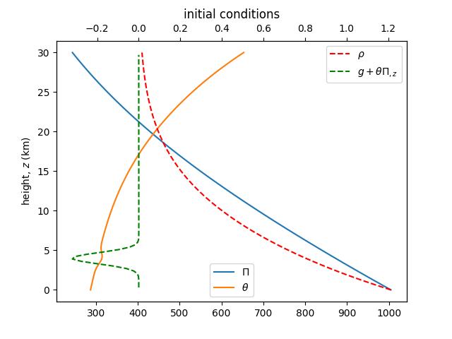
Figure 1: Initial vertical profiles for the 1D test case, which a potential temperature perturbation overlaying a state of hydrostatic balance.

In all cases we use a time step of $\Delta t=600s$, and 100 uniformly spaced elements, and boundary conditions on the bottom $z_{b}$ and top $z_{t}$ of the form $w|_{z_{b}}=w|_{z_{t}}=0$, $\partial\Pi/\partial z|_{z_{b}}=\partial\Pi/\partial z|_{z_{t}}=0$. No upwinding or other form of stabilisation was applied in any case, such that $c=0$ in (3a) and (3c). We explore results for two different formulations, one in which the matrix inverses are all computed directly, and the solvers are iterated to convergence, and a second using lumped matrix inverses (with the exception of the Helmholtz operator, which is solved directly), and just four Newton nonlinear iterations per time step, since in practice for large resolutions using parallel decompositions direct inverses are not practical. In each case the Helmholtz operator and all other matrices are assembled only once at the beginning of the time step.

Figure 2 shows the energy conservation error, Helmholtz matrix condition number, and number of nonlinear iterations to convergence for the different preconditioners using direct matrix inverses and iterating each time step to convergence below a tolerance of $10^{-14}$ for $|\delta\rho_{h}|/|\rho_{h}|$, $|\delta\mathcal{T}_{h}|/|\mathcal{T}_{h}|$, $|\delta\Pi_{h}|/|\Pi_{h}|$ for $\mathcal{T}_{h}\in\theta_{h},\Theta_{h}$ (we exclude the velocity residual from the convergence criteria, since the absolute values of this are small and somewhat volatile). While the original flux form preconditioner detailed in Section 3.1 and [5] fails after just 40 time steps, and the material form preconditioner fails after 527 time steps, the new flux form and energy conserving material formulation run stably for the full duration of the simulation (800 steps). The instability of the Charney-Phillips material form scheme is reflected in the long term growth in energy and more variation in the condition number of its Helmholtz operator. The condition number of the Charney-Phillips grid Helmholtz operator is generally lower than that for the Lorenz grid operators (albeit with much more variation), suggesting faster convergence for the inner linear solve. However the Charney-Phillips material form also requires on average more outer nonlinear iterations to achieve convergence. This is perhaps a result of the smaller condition number such that the Charney-Phillips grid operator may not span the eigenvalues of the true Jacobian as effectively as the Lorenz grid operators. The new flux form and energy conserving material formulation are very similar in all cases, with perhaps the main difference being in the condition number of the matrix at early times during the process of hydrostatic adjustment, suggesting that the new flux form will require fewer linear solver iterations for this regime.

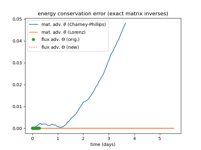
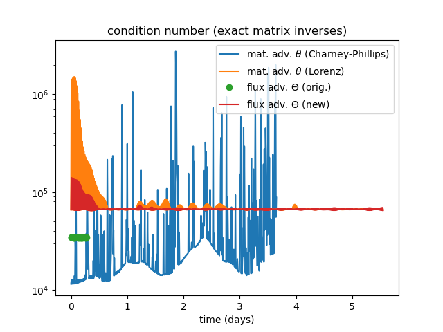
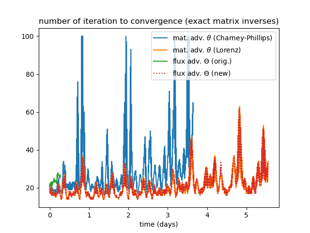
Figure 2: Energy conservation error (top), Helmholtz operator condition number (middle) and number of nonlinear iterations to convergence (bottom) for the three different preconditioners using exact matrix inverses.

For large scale applications on distributed memory computing architectures it is not feasible to directly compute matrix inverses, or to iterate to convergence, as for the configurations presented in Figure 2. Consequently all intermediate matrix inverses are replaced by lumped approximations, with the exception of the Helmholtz operator, and the resulting linear system is solved only a finite number of times per time step rather than to nonlinear convergence. Results using lumped matrix inverses and four Newton nonlinear iterations are presented in Figure 3 for the energy conservation errors, Helmholtz matrix condition number and residual errors (for the two formulations that ran stably to completion) at the final Newton iteration respectively. For this configuration both the material form preconditioner and the original flux form preconditioner are stable for only a small number of time steps (11 and 4 respectively), while once again the new flux form preconditioner and the energy conserving material formulation on the Lorenz grid are stable for the full 800 time steps with no sign of instability in the energy conservation error, condition number or residual error.

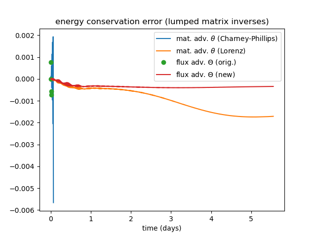
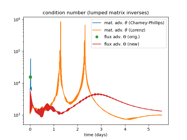
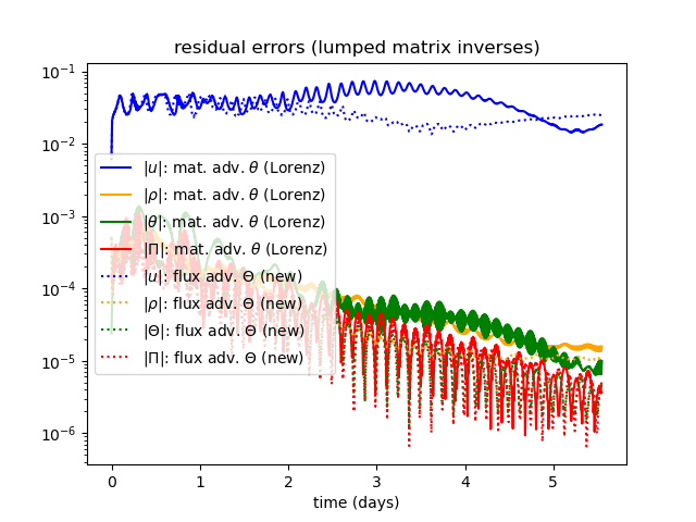
Figure 3: Energy conservation error (top), Helmholtz operator condition number (middle) and number of nonlinear iterations to convergence (bottom) for the three different preconditioners using exact matrix inverses.

Using only a finite number of nonlinear iterations the differences between the new flux form and energy conserving material formulations are more apparent. The material formulation shows more energy damping, as well as more variation in the matrix condition number, which is greater for moderate times, but lower for long times, perhaps due to the effects of the damped energy. The residual errors at the fourth Newton iteration are similar for both formulations, but marginally lower for the new flux formulation in most cases.

Since the new flux form preconditioner is applied to the same residuals (3) as the original flux form preconditioner as presented in Section 3.1, we can attribute the enhanced stability for both the converged and finite number of nonlinear iterations solutions to the new preconditioner.

4.2 2D non-hydrostatic gravity wave

In order to verify the new preconditioner, this is applied to the solution of a standard test case for a non-hydrostatic gravity wave travelling with an initial mean flow of $20ms^{-1}$ in the horizontal direction [25, 26, 3]. The domain is of size $[0,3\times 10^{5}]\times[0,10^{4}]m$ and is discretised using $300\times 10$ lowest order elements and is run for a simulation time of $3000s$ using a time step of $\Delta t=20s$.

The gravity wave is driven by an initial perturbation to an otherwise hydrostatically balanced potential temperature profile of the form

$$\theta_{p}(t=0)=\frac{0.01\sin(\pi z/H)}{1+(x-x_{c})^{2}/a_{c}^{2}}\ ,$$ (29)

where $H=10^{4}m$ is the domain height, $a_{c}=5\times 10^{3}m$, $x_{c}=10^{4}m$ is the center of the perturbation, while the initial mean potential temperature is given as a function of the Brunt-Väisälä frequency $\mathcal{N}=0.01s^{-1}$ as $\theta_{m}(t=0)=\theta_{0}e^{\mathcal{N}^{2}z/g}$, where $\theta_{0}=300^{\circ}K$. The initial Exner pressure and density profiles are given respectively as

$$\Pi(t=0)=c_{p}+\frac{g^{2}(e^{-\mathcal{N}^{2}z/g}-1)}{\theta_{0}\mathcal{N}^{2}}\ ,$$ (30)

and

$$\rho(t=0)=\frac{p_{0}}{R\theta_{m}}\Bigg{(}\frac{\Pi}{c_{p}}\Bigg{)}^{c_{v}/R}\ ,$$ (31)

while the initial density weighted potential temperature given as $\Theta=\rho(\theta_{m}+\theta_{p})$. See the appendix for a full description of the constants above. In order to ensure an initial state of hydrostatic balance, these initial conditions are applied as finite element projections, rather than analytic functions.

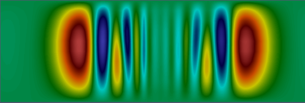
Figure 4: Potential temperature perturbation from the mean initial state, $\theta_{p}=\theta-\theta_{m}(t=0)$ at time $3000s$ for the 2D non-hydrostatic gravity wave test case (projected from discontinuous space $\mathbb{W}_{3}$ to continuous space $\mathbb{W}_{0}$). Colors range from $-0.00162^{\circ}K$ to $+0.00265^{\circ}K$. Vertical axes is scaled by a factor of 10 with respect to the horizontal.

The perturbed potential temperature (difference between the current value and the mean initial value, $\theta_{m}$) is given at time $3000s$ in Figure 4. Since this is represented on the discontinuous piecewise constant space $\mathbb{W}_{3}$ within the model, for clarity this is projected into the continuous piecewise linear space $\mathbb{W}_{0}$ in the figure. Despite the low resolution of the test configuration and long time step, this agrees well with a previous high resolution solution [26], both in terms of position and amplitude of the disturbance.

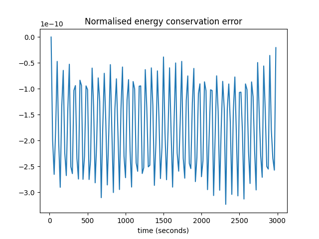
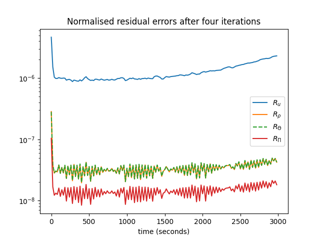
Figure 5: Energy conservation error (top), and residual errors after four nonlinear iterations (bottom) for the 2D non-hydrostatic gravity wave test case.

The energy conservation and residual errors on the fourth Newton iteration as a function of time are given in Figure 5. There is no observable drift in the energy conservation error, while the residual errors increase somewhat as the solution evolves, indicating that the solution is perhaps slightly under-damped. Both exhibit an oscillation on a time scale of $2\Delta t$, perhaps due to the presence of acoustic modes, which are not explicitly resolved for a spatial resolution of $\Delta x=1000m$ and a time step of $\Delta t=20s$.

4.3 2D rising bubble

The new preconditioner is further verified against a modified version of a standard test case [27] for a rising thermal bubble within an otherwise isothermal, hydrostatic atmosphere [26]. The model is run on a domain of size $[0,1000]\times[0,1500]m$ using $288\times 432$ lowest order elements and a time step of $\Delta t=2.5s$ for a total of $1200s$. The dynamics are driven by a perturbation of the potential temperature of the form

$$\theta_{p}=0.25(1+\cos(r\pi/250))\quad r\leq 250\ ,$$ (32)

where $r^{2}=(x-500)^{2}+(y-260)^{2}$, against an isothermal background state of $\theta_{0}=300K$.

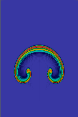
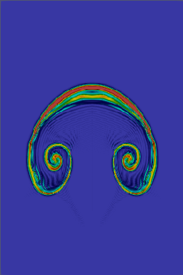
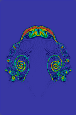
Figure 6: Potential temperature, $\theta$ at times $800s$ (left), $1000s$ (center) and $1200s$ (right) for the 2D warm bubble test case. Colors range from $300^{\circ}K$ to $300.5^{\circ}K$.

Figure 6 shows the potential potential temperature field at times $800s$, $1000s$ and $1200s$ respectively. While the overall shape of the bubble compares well against previous results [26], the evolution of the bubble is somewhat delayed compared to those results, and the secondary instability is slightly different. This is perhaps due to the lower polynomial order, the absence of upwinding or monotonicity, as well as the application of the APVM term, which while energy conserving, is also known to be inconsistent with respect to the original continuous system (1) [28]. Also there is an oscillatory tail that develops in the wake of the bubble, owing to the absence of upwinding in (3c). Nevertheless, the continuous interior penalty term (6) and APVM are effective at stabilising the simulation, as reflected in the temporal profile of the energy conservation error as given in Figure 7. This figure also gives the residual errors after four nonlinear iterations as a function of time. While these reduce throughout the course of the simulation, there is a slight upturn in the residual and energy conservation errors at long times, which first appear in the velocity and density residuals, suggesting that the simulation may ultimately go unstable over very long times, and that the interior penalty term may be somewhat under-damped.

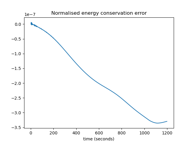
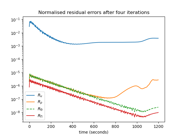
Figure 7: Energy conservation error (top), and residual errors after four nonlinear iterations (bottom) for the 2D warm bubble test case.

5 Conclusions

A new Helmholtz preconditioner for the compressible Euler equations with flux form density weighted potential temperature transport on the Lorenz grid using mixed finite elements is presented. A transformation of the density and density weighted potential temperature residuals into a material transport equation for the thermodynamic entropy allows the new preconditioner to preserve a similar block structure as an existing preconditioner for the material transport of potential temperature on the Charney-Phillips grid. One dimensional comparisons against this and another previous formulation for material form transport on the Lorenz grid show the new preconditioner to be more stable, both when run to convergence using exact matrix inverses and for when using just four Newton nonlinear iterations per time step with approximate lumped matrix inverses within the compound Helmholtz operator. Comparisons to an alternative energy conserving formulation for material form potential temperature transport on the Lorenz grid show little variation for converged solutions, but less energy damping and lower condition numbers for a finite number of nonlinear iterations.

The new preconditioner is further verified for existing two dimensional test cases within vertical slice configurations. For these more challenging configurations a continuous interior penalty term is introduced in order to damp grid scale jumps in the mass flux gradient by way of kinetic energy dissipation.

Appendix: Vertical profiles for the hydrostatically balanced 1D atmosphere

The 1D vertical profiles are taken from [24]. Constants are given as: $T_{e}=310K$, $T_{p}=240K$, $g=9.80616ms^{-2}$, $\gamma=0.005Km^{-1}$, $p_{0}=10^{5}Pa$, $c_{p}=1004.5Jkg^{-1}K^{-1}$, $R=287Jkg^{-1}K^{-1}$. In order to determine the reference profiles, we first introduce some intermediate variables as:

$$T_{0} =(T_{e}+T_{p})/2$$ (33a)

$$B =(T_{e}-T_{p})/((T_{e}+T_{p})T_{p})$$ (33b)

$$C =5(T_{e}-T_{p})/(2T_{e}T_{p})$$ (33c)

$$D =\cos^{3}(2\pi/9)-(3/5)\cos^{5}(2\pi/9)$$ (33d)

$$E =(gz/(2RT_{0}))^{2}$$ (33e)

$$\tau_{1} =T_{0}^{-1}e^{\gamma z/T_{0}}+B(1-2E)e^{-E}$$ (33f)

$$\tau_{2} =C(1-2E)e^{-E}$$ (33g)

$$\chi_{1} =\gamma^{-1}(e^{\gamma z/T_{0}}-1)+Bze^{-E}$$ (33h)

$$\chi_{2} =Cze^{-E}\ .$$ (33i)

From the intermediate values given above, the initial vertical profiles for the temperature, pressure, Exner pressure, density and potential temperature may be given respectively as

$$T =(\tau_{1}-\tau_{2}D)^{-1}$$ (34a)

$$p =p_{0}e^{-g\chi_{1}/R+g\chi_{2}D/R}$$ (34b)

$$\Pi =c_{p}(p/p_{0})^{R/c_{p}}$$ (34c)

$$\rho =p/(RT)$$ (34d)

$$\theta =T(p_{0}/p)^{R/c_{p}}\ .$$ (34e)

References

- [1] K-S Yeh, J Côté, S Gravel, A Méthot, A Patoine, M Roch and A Staniforth. The CMC-MRB Global Environmental Multiscale (GEM) Model. Part III: Nonhydrostatic Formulation. Mon. Wea. Rev., 130:339–356, 2002.
- [2] N Wood, A Staniforth, A White, T Allen, M Diamantakis, M Gross, T Melvin, C Smith, S Vosper, M Zerroukat and J Thuburn. An inherently mass-conserving semi-implicit semi-Lagrangian discretization of the deep-atmosphere global non-hydrostatic equations. Q. J. R. Meteorol. Soc., 140:1505–1520, 2014.
- [3] T Melvin, T Benacchio, B Shipway, N Wood, J Thuburn, and C Cotter. A mixed finite-element, finite-volume, semi-implicit discretisation for atmospheric dynamics: Cartesian geometry. Q. J. R. Meteorol. Soc., 145:1–19, 2019.
- [4] C Maynard, T Melvin, and E H Müller. Multigrid preconditioners for the mixed finite element dynamical core of the LFRic atmospheric model. Q. J. R. Meteorol. Soc., 146:3917–3936, 2020.
- [5] D Lee. An energetically balanced, quasi-Newton integrator for non-hydrostatic vertical atmospheric dynamics. J. Comp. Phys., 429:109988, 2021.
- [6] D Lee and A Palha. Exact spatial and temporal balance of energy exchanges within a horizontally explicit/vertically implicit non-hydrostatic atmosphere. J. Comp. Phys., 440:110432, 2021.
- [7] S Reddy, M Waruszewski, F A V de Braganca Alves, and F X Giraldo. Schur complement IMplicit-EXplicit formulations for discontinuous Galerkin non-hydrostatic atmospheric models. J. Comp. Phys., 491:112361, 2023.
- [8] T H Gibson, L Mitchell, D A Ham, C J Cotter. Slate: extending Firedrake’s domain-specific abstraction to hybridized solvers for geoscience and beyond. Geosci. Model. Dev., 13:735–761, 2020.
- [9] J D Betteridge, C J Cotter, T H Gibson, M J Griffiths, T Melvin and E H Müller. Hybridised multigrid preconditioners for a compatible finite-element dynamical core. Q. J. R. Meteorol. Soc., 149:2454–2476, 2023.
- [10] A Arakawa and C S Connor. Vertical differencing of the primitive equations based on the Charney-Phillips grid in hybrid vertical coordinates. Mon. Wea. Rev., 124:511–528, 1996.
- [11] J Thuburn and T J Woolings. Vertical discretizations for compressible Euler equation atmospheric models giving optimal representation of normal modes J. Comp. Phys., 203:386–404, 2005.
- [12] T M Bendall, T H Gibson, J Shipton, C J Cotter, B Shipway. A compatible finite-element discretisation for the moist compressible Euler equations. Q. J. R. Meteorol. Soc., 146:3187–3205, 2020.
- [13] T Melvin, T Benacchio, J Thuburn, and C Cotter. Choice of function spaces for thermodynamic variables in mixed finite-element methods Q. J. R. Meteorol. Soc., 144:900–916, 2018.
- [14] M A Taylor, O Guba, A Steyer, P A Ullrich, D M Hall, and C Eldred. An Energy Consistent Discretization of the Nonhydrostatic Equations in Primitive Variables. Journal of Advances in Modelling Earth Systems, 12:(1), 2020.
- [15] C Eldred, T Dubos, and E Kritsikis. A quasi-Hamiltonian discretization of the thermal shallow water equations. J. Comp. Phys., 379:1–31, 2019.
- [16] K Ricardo, D Lee, and K Duru. Entropy and energy conservation for thermal atmospheric dynamics using mixed compatible finite elements J. Comp. Phys., 496:112605, 2024
- [17] A Natale, J Shipton, and C J Cotter. Compatible finite element spaces for geophysical fluid dynamics. Dyn. Stat. Climate Sys., 1:1–31, 2016.
- [18] W Bauer and C J Cotter. Energy–enstrophy conserving compatible finite element schemes for the rotating shallow water equations with slip boundary conditions. J. Comp. Phys., 373:171–187, 2018.
- [19] E Burman and A Ern. Continuous interior penalty -finite element methods for advection and advection-diffusion equations. Mathematics of Computation, 76:1119–1140, 2007.
- [20] R Sadourny, C Basdevant. Parameterization of Subgrid Scale Barotropic and Baroclinic Eddies in Quasi-geostrophic Models: Anticipated Potential Vorticity Method J. Atmos. Sci., 42:1353–1363, 1985.
- [21] J Thuburn. Numerical entropy conservation without sacrificing Charney–Phillips grid optimal wave propagation. Q. J. R. Meteorol. Soc., 148:2755–2768, 2022.
- [22] S. Badia and F. Verdugo. Gridap: An extensible finite element toolbox in Julia. J. Open Source Softw., 5:2520, 2020.
- [23] S. Badia, A. F. Martín, and F. Verdugo. GridapDistributed: a massively parallel finite element toolbox in Julia. J. Open Source Softw., 7:4157, 2022.
- [24] P A Ullrich, T Melvin, C Jablonowski, and A Staniforth. A proposed baroclinic wave test case for deep‐ and shallow‐atmosphere dynamical cores. Q. J. R. Meteorol. Soc., 140:1590–1602, 2014.
- [25] W C Skamarock and J B Klemp. Efficiency and Accuracy of the Klemp-Wilhelmson Time-Splitting Technique. Mon. Wea. Rev., 122:2623–2630, 1994.
- [26] F X Giraldo and M Restelli. A study of spectral element and discontinuous Galerkin methods for the Navier–Stokes equations in nonhydrostatic mesoscale atmospheric modeling: Equation sets and test cases. J. Comp. Phys., 227:3849–3877, 2008.
- [27] A Robert. Bubble convection experiments with a semi-implicit formulation of the Euler equations. J. Atmos. Sci., 50:1865–1873, 1993.
- [28] D Lee, A Martin, C Bladwell, and S Badia. A comparison of variational upwinding schemes for geophysical fluids, and their application to potential enstrophy conserving discretisations in space and time. arXiv 2203:04629, 2022.