Galaxies lensing quadruply imaged quasars lie close to the centers of their lensing potentials

Abstract

In modeling the potentials of quadruply lensed quasars, investigators often employ models for the stellar surface brightness profile of the lensing galaxy for the sole purpose of eliminating its contamination of the light from the quasar images and their hosts. When the center of that profile is used, it is usually as a weak prior on the center of the potential. But the central maxima in the light from single lensing galaxies lie closer the centers of the lens potentials than has heretofore been thought. New measurements are presented here of the positions of the compact central regions of lensing galaxies observed with the Hubble Space Telescope. Comparing these with modeled positions for the centers of the lensing potential (constrained only by the positions of the four quasar images) we find agreement consistent with the larger of either our measurement uncertainties or 1% of the radius of the Einstein ring.

1 Eliminate free parameters when you can

A model for a quadruply lensed quasar (or supernova) includes both a model for the lensed object (a point source, and sometimes an extended host) and a model for the gravitational potential that deflects light from the source. However small the number of parameters for a particular model might be, one would almost always choose to eliminate a free parameter if doing so did not introduce an unmanageable systematic error.

Modelers frequently forego constraining the center of the potential with the observed center of the lensing galaxy with good reason. There are numerous cases where the two are not coincident, from the Local Group to lensing galaxies in cluster environments. In their paper on automated lens modeling, Ertl et al. (2023) adopt a prior on the centers of their lensing potentials that is more than a hundred times larger than the GAIA calibrated uncertainty with which they measure the centers of their lensing potentials.

In this paper, we demonstrate that, for the case of point sources quadruply lensed by relatively isolated galaxies, they coincide more closely than has heretofore been thought. The principal result of this paper the specification of a prior for use in modeling of such systems.

In what follows, we make extensive use of the results of Witt (1996), Wynne & Schechter (2018), and Schechter & Wynne (2019), who show that for the singular isothermal elliptical potential (henceforth SIEP), the four images of a quadruply lensed quasar are the intersection points of a uniquely determined rectangular hyperbola and an ellipse. Both the source and the center of the potential lie on the same (“primary”) branch of the hyperbola, and the ellipse is centered on the source. Luhtaru et al. (2021) give a detailed argument that the Witt-Wynne construction also works for a family of models comprised of an SIEP with shear centered on the source and parallel to the flattening of the potential (henceforth SIEP+XS_∥).

Consequently, the Witt-Wynne construction (using only the four image positions) predicts a one-dimensional locus (a hyperbola) for the center of the potential. By showing that the observed center of most systems lies close to the hyperbola, we provide evidence that the observed center also lies close to the center of the potential. Although this method strictly demonstrates closeness in only one dimension, the two centers must be close in both dimensions if we assume the projection axis is randomly oriented.

We did not set out to study the centrality of lensing galaxies. It emerged from an effort on our part to improve upon the measurements of the relative importance of the relative contributions of the flattening of lens galaxies and the tidal shear from neighboring galaxies to the quadrupole moment of the potential, following the method developed by Luhtaru et al. (2021). We relegate the description of that effort to Appendix A, as it is rather technical and of interest primarily to lens modelers. The most reliable positions for the centers of the potentials and lensing galaxies found in the Appendix are used in the main body of this paper to determine the degree of centrality of the lensing galaxies.

2 Two quasars predict a unique galaxy position

If a system is perfectly modeled by a family of SIEP+XS_∥ models, the four images detemine a unique rectangular hyperbola on which the galaxy potential lies but not its location on that hyperbola. If the system includes a second multiply lensed quasar, there is a second, distinct Witt-Wynne construction, each with its own hyperbola. The center of the SIEP must lie where the two hyperbolae intersect.

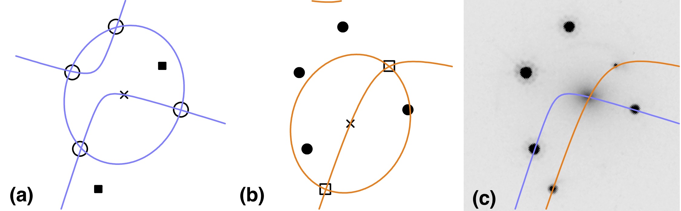
Figure 1: The Witt-Wynne construction for PS J1721+88. Panel (a) shows the four images of one of the two quasars as open circles. Panel (b) shows the two images of the other source as open squares. The centers of the ellipses are marked with an $x$ on each of the primary branches of the hyperbolae. The secondary branch of the doubly lensed quasar is just visible at the top of panel (b). The lensing galaxy, whose position was not used in the construction, is predicted to lie at the intersection of the two primary branches, and is shown in panel (c), an HST F814W image of the system.

The gravitationally lensed quasar system PS J1721+88 (Lemon et al., 2018) is very nearly such a case, with one galaxy lensing two quasars, one quadruply and the other doubly, and is shown in Figure 1.

The Witt-Wynne construction for the doubly lensed quasar, shown in Figure 1b, proceeded as follows. First, the Wynne ellipse for the quadruply lensed quasar was translated parallel to itself until it passed through the two quasar images. Then we found the rectangular hyperbola with the same semi-major axis and orientation as the first Witt hyperbola that passed through the center of the second Wynne ellipse (with the secondary branch of Witt’s hyperbola at the very top of the panel).

In Figure 1c, we show the two hyperbolae superposed on an HST F814W image of the system. The observed center of the lensing galaxy lies very close to the intersection of the two hyperbolae, whose locii were determined only by the positions of the quasar images.

The authors acknowledge that confirmation bias is at work in our decision to present this case, but it is the only system lensing two quasars that is presently known.

3 New Shear/Ellipticity Decompositions and “Centralities”

Luhtaru et al. (2021) analyzed 39 systems with a single lensing galaxy inside the Einstein radius of the system. They used SIEP + XS_|| models,

$$\psi(b,\eta,\gamma)=b\sqrt{q_{pot}x^{2}+\frac{y^{2}}{q_{pot}}}-\frac{\gamma}{2}(x^{2}-y^{2})\,.$$ (1)

where $\psi$ is the dimensionless prodected potential and $\gamma$ is the shear. They define a “semi-ellipticity”, $\eta$, such that

$$q_{pot}=(1-\eta)/(1+\eta)\quad,$$ (2)

and an “effective quadrupole”, $\Gamma_{eff}$,

$$\Gamma_{eff}\equiv\frac{\gamma+\eta}{1+\gamma\eta}\quad,$$ (3)

in which $\gamma$ and $\eta$ enter interchangeably. $\Gamma_{eff}\approx\eta+\gamma$ for values of the semi-ellipticity and shear typical of quadruply lensed quasars.

The effective quadrupole is tightly constrained by the elongation of the image configuration. The parameter $b$, roughly equal to the Einstein radius, $\theta_{E}$, is also well constrained by the four quasar images. By contrast, the ratio of the semi-ellipticity to the shear, by construction, is unconstrained. We have $\eta\approx\Gamma_{eff}-\gamma$.

In Table 3 we give new shear/ellipticity decompositions for all of the systems analyzed by Luhtaru et al. (2021). They incorporate the new measurements reported in Appendix A.

As discussed at length in A, one can measure the position of the center of a lensing galaxy with a precision of roughly $0\farcs 005$. This varies from system to system depending upon details of the the lens’ surface brightness distribution.

The entries for $d\gamma$, the uncertainty in the shear, (and also in semi-ellipticity $\eta$) has been recalculated taking into account a generic $0\farcs 005$ measurement uncertainty in the positions measured for all of lenses. This is specific to the measurement scheme described in the appendix, but was otherwise typical of the uncertainties estimated in the fitting program, clumpfit.

For each system we give the measured perpendicular offset $D_{\perp}$ of the lens position from Witt’s hyperbola. We assume (not quite correctly) that the offset along the hyperbola of the true center of the potential, $D_{\parallel}$, is equal to $D_{\perp}$. The uncertainty along the hyperbola is then given by

$$\Delta D_{\parallel}\approx\sqrt{(0\farcs 005)^{2}+D_{\perp}^{2}}\quad.$$ (4)

Taking the uncertainty $\Delta D_{\perp}$ to be equal to $\Delta D_{\parallel}$ and normalizing these by $b$ the strength of the lens, we have

$$\Delta\left(\frac{D_{\perp}}{b}\right)\approx\sqrt{\left(\frac{0\farcs 005}{b}\right)^{2}+\left(\frac{D_{\perp}}{b}\right)^{2}}\quad,$$ (5)

and adopt the word “centrality” for the quantity on the left hand side. This definition is specific to the SIEP+XS_∥ model.

Table 1: Estimated shear and ellipticity values of all 39 analyzed single-lens systems, observed lens offsets and centralities

System name	$\gamma$		$\eta$		$\Delta\gamma$		$\Gamma_{\text eff}$	$D_{\perp}(\arcsec)$	$\Delta\left(\frac{D_{\perp}}{b}\right)$	ref
J0029-3814	0.445	-0.113	0.016	0.350	0.011	0.015	1
J0030-1525	-0.034	0.100	0.002	0.066	0.002	0.005	1
PS J0147+4630	0.180	-0.020	0.017	0.160	0.063	0.033	2
SDSS J0248+1913	0.120	-0.020	0.012	0.100	0.005	0.009	2
ATLAS J0259-1635	0.031	0.038	0.062	0.069	0.020	0.028	2
DES J0405-3308	-0.011	0.034	0.051	0.023	0.014	0.021	2
DES J0420-4037	0.000	0.034	0.004	0.034	0.002	0.007	2
HE0435-1223	0.049	0.026	0.019	0.075	0.008	0.008	3
J0530-3730	0.088	0.040	0.026	0.128	0.017	0.030	1
J0659+1629	0.013	0.066	0.033	0.079	0.077	0.032	1
B0712+472	0.078	0.028	0.003	0.106	0.001	0.007	4
HS0810+2554	0.011	0.008	0.051	0.019	0.015	0.034	3
RXJ0911+0551	0.271	0.030	0.003	0.299	0.001	0.004	3
SDSS0924+0219	0.041	0.017	0.005	0.058	0.000	0.006	3
J1042+1641	-0.028	0.056	0.044	0.028	0.035	0.040	5
PG1115+080	0.109	0.001	0.009	0.110	0.007	0.007	3
RXJ1131-1231	0.118	0.020	0.011	0.138	0.036	0.020	3
J1131-4419	0.002	0.031	0.007	0.033	0.004	0.008	1
J1134-2103	0.295	0.045	0.066	0.336	0.042	0.033	1
SDSS1138+0314	0.110	-0.010	0.019	0.100	0.004	0.010	3
SDSS J1251+2935	0.053	0.053	0.005	0.105	0.005	0.008	2
HST12531-2914	0.258	-0.088	0.081	0.174	0.009	0.017	3
SDSS J1330+1810	-0.030	0.078	0.012	0.048	0.005	0.008	6
HST14113+5211	0.260	0.015	0.077	0.273	0.022	0.026	3
H1413+117	0.137	-0.027	0.155	0.110	0.033	0.054	3
HST14176+5226	0.162	0.000	0.144	0.162	0.075	0.053	3
B1422+231	0.174	0.057	0.006	0.229	0.007	0.011	3
SDSS J1433+6007	0.197	0.001	0.038	0.198	0.071	0.041	2
J1537-3010	0.209	-0.062	0.045	0.148	0.004	0.004	1
PS J1606-2333	0.234	-0.026	0.139	0.209	0.033	0.047	2
J1721+8842	0.108	0.013	0.008	0.121	0.016	0.008	1
J1817+27	-0.095	0.120	0.091	0.025	0.051	0.057	1
WFI2026-4536	0.115	-0.008	0.037	0.107	0.013	0.021	3
DES J2038-4008	0.035	0.056	0.007	0.091	0.006	0.006	2
B2045+265	0.145	0.018	0.005	0.163	0.014	0.013	7
J2100-4452	0.034	0.037	0.012	0.071	0.014	0.011	1
J2145+6345	0.112	0.038	0.061	0.150	0.062	0.062	1
J2205-3727	0.041	0.038	0.004	0.079	0.000	0.007	1
WISE J2344-3056	-0.168	0.232	0.016	0.067	0.001	0.010	2

References. — (1)Luhtaru et al. (2021); (2) newly measured, Table A1; (3) Kochanek et al. (1999); (4) Hsueh et al. (2017); (5) Glikman et al. (2018); (6) Rusu et al. (2016); (7) McKean et al. (2007)

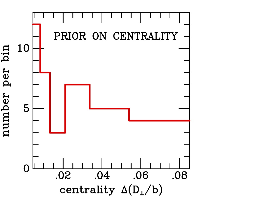
Figure 2: A prior on the centralities, $\Delta\left(\frac{D_{\perp}}{b}\right)$, defined in equation (5), can be constructed from the observed offsets, $D_{\perp}$, for each of the 39 systems analyzed by Luhtaru et al. (2021) and constructing a histogram. One then scales the values on the abscissa by the total number of systems. For each centrality bin, the prior is taken to be a Gaussian whose width is specified by that scaled abscissa. The binning is logarithmic, with each bin 1.6 times wider than the previous bin. Half of the systems analyzed by Luhtaru et al. have centralities less than 0.01.

In Figure 2 we show a histogram of the centralities, $\Delta\left(\frac{D_{\perp}}{b}\right)$, for the 39 relatively isolated systems studied by Luhtaru et al. (2021). The histogram can be used to construct a prior on centralities by first scaling the abscissa by the total number of systems and then taking the prior on each bin to be a Gaussian whose width is given by the abscissa. The bins are logarithmic, with each spanning a factor of 1.6 in centrality. Half of the Luhtaru et al. systems have (dimensionless) centralities of less than $0.01$.

4 The centrality of quadruply lensing galaxies

The histogram of Figure 2 constitutes the principal result of this paper. Galaxies that are both relatively isolated and produce four quasar images lie very close to the centers of the lensing potential if it is modeled by a singular isothermal elliptical with parallel external shear.

Small though the observed offsets may be, they are much larger than the normalized rms differences between the GLEE measurements and the clumpfit measurements described in Appendix A. Most of the offset of isolated lensing galaxies from Witt’s hyperbola must therefore be due to errors in the Witt-Wynne model. These errors are typically only 1% of the size of the Einstein ring.

5 Conclusions

We have shown when a relatively isolated galaxy produces a quadruply lensed quasar, its center is closer to the center of the potential than has heretofore been thought. This permits the use of stronger priors in the modeling of such systems, with an attendant reduction in the uncertainties in model parameters. We suggest a prior on a quantity that we call centrality, defined with respect to the Witt-Wynne model.

Appendix A New measurements of the centers of galaxies quadruply lensing quasars

A.1 Why astrometric accuracy needs improvement

We did not set out to study the centrality of lensing galaxies. Our finding emerged from an effort to improve upon the estimate of the relative contributions of flattening of lens galaxies and tidal shear to the quadrupole moments potentials obtained by Luhtaru et al. (2021). Their method is succinctly summarized in Section 1.

It is limited by the accuracy with which one can measure the positions of the quasar images and the position of the lensing galaxy, which is assumed to have a singular isothermal elliptical potential with parallel external shear (SIEP+XS_∥). The uncertainty in flattening/shear decomposition is estimated from the offset the lensing galaxy from the Witt (1996) hyperbola.

Luhtaru et al. concluded that shear contributes roughly twice as much as galaxy flattening to the “effective shear”, $\Gamma_{eff}$, the overall quadrupole component of a potential that quadruply lenses a quasar. Were the uncertainties in their adopted positions larger than reported, the reliability of that conclusion might be challenged.

Measuring positions for the four images of a quadruply lensed quasar is less clear cut than one might at first imagine. The quasars are embedded in host galaxies and their images are projected onto the lensing galaxies. Perfect modeling of an exposure must take into account the point spread function, the various shapes and sizes of galaxies (lenses and quasar hosts), and the gravitational potential that produces four images from a single quasar and host. While multiple software suites are widely available to analyze quadruply lensed quasar systems, each of them incorporates different choices in accounting for these the relative importance of these features.

A.2 Discrepant reports of image and lens center positions

Ertl et al. (2023) compared positions for the images of nine quadruply lensed quasars measured using two different automated schemes on the same set of HST images. One of those was a version of Lenstronomy developed by Schmidt et al. (2023) and described therein. The other was a version of GLEE, developed and described by Ertl et al. (2023)

After discarding one extremely discrepant system, the rms differences in the quasar image positions differed by $0\farcs 006$ and $0\farcs 005$ in right ascension and declination. This was larger than had been anticipated. Comparing the GLEE results with astrometry from Gaia DR3 (Gaia Collaboration et al., 2021), Ertl et al. reported differences of $0\farcs 0017$ and $0\farcs 0023$, respectively.

Luhtaru et al. (2021) was based on astrometry drawn from the literature, much of it from the CASTLES (Kochanek et al., 1999) data base. They also reported new measurements on thirteen recently acquired HST exposures. They described their measurements, using a program called clumpfit, as “preliminary” deferring to the anticipated measurements by Schmidt et al. (2023) which they called “authoritative.” Ertl et al. compared their GLEE astrometry with the “preliminary” results of Luhtaru et al. (2021), they found rms differences marginally smaller than with Gaia DR3, $0\farcs 0017$ in each direction. It would therefore seem that Luhtaru et al. were mistaken in deferring to the Schmidt et al. (2023) measurements.

Luhtaru et al. also used measurements for ten systems reported by Shajib et al. (2019) which were obtained with an earlier version of lenstronomy. If the errors in these were as large as those of the Schmidt et al. (2023) astrometry, the Luhtaru et al. conclusion regarding the relative importance of shear and ellipticity might be compromised. We therefore remeasured, using clumpfit, the same ten HST images analyzed by Shajib et al. (2019).

In comparing clumpfit and GLEE, we were impressed that the agreement for some systems was better than $0\farcs 001$. With positions this good, the uncertainties in the modeled centers of the potentials would be correspondingly accurate. This motivated us to compare the clumpfit positions for the maximum in lens surface brightness with the theoretical centers for the potential computed from the positions of the quasar images.

A.3 New clumpfit astrometry

The Luhtaru et al. (2021) measurements were carried out with the program clumpfit described briefly in Agnello et al. (2018). It incorporates elements of DoPHOT (Schechter et al., 1993), fitting point sources with either an elliptical “pseudo-Gaussian” or a lookup table taken from a nearby star. Galaxies are fit with elliptical pseudo-Gaussians. These do not allow for curved images and so is ill suited toward modeling the images of quasar hosts. The clumpfit model does not couple the images to a lensing potential, which can be modeled subsequently using the image parameters.

We used nearby stars as PSF templates when possible. Unfortunately there were no stars on the HST images sufficiently bright for this purpose for the majority of systems, so we used pseudo-Gaussians. For some of the systems for which PSF templates were available we nevertheless tried pseudo-Gaussians and found no substantial differences.

The position of the lensing galaxy is of primary importance in distinguishing between ellipticity and shear, so the clumpfit residuals were examined for effects that might influence the position of the lensing galaxy.

The two greatest concern were that a) the very substantial residuals from the four point sources would “pull” or “push” the outer isophotes of the much lower surface brightness lensing galaxy and b) that the unmodeled flux from the quasar host might similarly pull those isophotes.

To minimize this effect, the lensing galaxy was often taken to be smaller than its isophotes would indicate, so as to weight the light from the center of the lens more heavily. In some cases, the width of the pseudo-Gaussian model was fixed at a value smaller than the best fitting value. In others, the lens galaxy was taken to have the PSF of a stellar template. Either way, the central intensity of the model for the starlight was adjusted by hand to exactly account for the flux at the center of the lens.

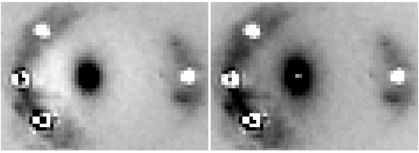
Figure 3: The left and right panels show residuals at the same contrast from fits of two different models to an HST F814W exposure of J1251+29. In the left panel, the lensing galaxy was taken to be an elliptical pseudo-Gaussian. In the right panel, it was taken to be a point source producing zero residual flux in the central pixel. The residuals in the left panel are asymmetric, the result of the outer isophotes of the elliptical Gaussian having been pulled toward the extended structure of the quasar host.

The effect is illustrated in Figure 3, which shows results from two alternative fits of surface brightness profiles to an HST F814 image of the lensed quasar system J1251+29. The left panel shows residuals when stellar PSFs are fit to the four images and the central galaxy is taken to be a unconstrained elliptical pseudo-Gaussian. Note that the galaxy has been pulled toward the extended structure of the quasar host, leaving positive residuals at the center of the lensing galaxy and negative residuals toward the triplet of quasar images. Using this fit, Luhtaru et al. (2021) found the system to be shear-dominated.

The right panel shows residuals from the fit of the stellar PSF to the center of the galaxy, with the amplitude constrained to give zero residual in the brightest pixel. The resulting center is our best estimate of the true position, giving shear and ellipticity contributing equally. This result is still somewhat suspect, as the angle of the resultant quadrupole lies very close to the position angle of the isophotes of the lensing galaxy.

The lesson to be learned (or reinforced) from Figure 3 is that residuals tell you more than side-by-side comparisons of models and data.

As we worked through the sample, system by system, to improve upon derived centroids, different schemes were developed on an ad hoc basis. The effects of imperfect point source subtraction on the lens position could in some cases be minimized by measuring an F475X exposure rather than the F814W exposure, but we this was done only when the F814W frame gave a suspect result. For some systems the lensing galaxy was too faint to make the F475X exposure useful. Each of the ten systems for which we present results was therefore treated slightly differently, depending upon the particular circumstances.

Table 2: Newly measured relative positions for galaxies and images of quadruply lensed quasars

	Image A				Image B				Image C			Image D		Galaxy
System name	$\Delta\alpha\cos\delta$		$\Delta\delta$		$\Delta\alpha\cos\delta$		$\Delta\delta$		$\Delta\alpha\cos\delta$		$\Delta\delta$	$\Delta\alpha\cos\delta$	$\Delta\delta$	$\Delta\alpha\cos\delta$	$\Delta\delta$
	($\arcsec$)		($\arcsec$)		($\arcsec$)		($\arcsec$)		($\arcsec$)		($\arcsec$)	($\arcsec$)	($\arcsec$)	($\arcsec$)	($\arcsec$)
PS J0147+4630	$0.0000$	$0.0000$	$1.1697$	$-0.4141$	$-1.2404$	$-0.0993$	$-0.3394$	$-3.2351$	$-0.1650$	$-2.0671$
SDSS J0248+1913	$0.0000$	$0.0000$	$-0.1472$	$-0.8344$	$0.8543$	$-1.4463$	$0.9050$	$-0.0366$	$0.4905$	$-0.6361$
ATLAS J0259-1635	$0.0000$	$0.0000$	$-0.3192$	$0.8789$	$-1.4736$		$-0.7163$	$-0.3845$	$-0.6812$	$0.2950$
DES J0405-3308	$0.0000$	$0.0000$	$-1.0656$	$-0.3261$	$-0.3416$	$0.8332$	$-1.2232$	$0.6967$	$-0.7007$	$0.2364$
DES J0420-4037	$0.0000$	$0.0000$	$0.2432$	$1.0271$	$0.8732$	$1.1431$	$1.4018$	$-0.2268$	$0.6938$	$0.3468$
SDSS J1251+2935	$0.0000$	$0.0000$	$0.2913$	$0.9626$	$0.3581$	$0.3756$	$-1.4249$	$0.9553$	$-0.3459$	$0.6239$
SDSS J1433+6007	$0.0000$	$0.0000$	$2.0455$	$1.5804$	$0.0017$	$3.7554$	$-0.7599$	$1.6262$	$0.9332$	$1.7008$
PS J1606-2333	$0.0000$	$0.0000$	$-1.6211$	$-0.5888$	$-0.7919$	$-0.9052$	$-1.1278$	$0.1504$	$-0.8345$	$-0.3669$
DES J2038-4008	$0.0000$	$0.0000$	$1.5128$	$-0.0274$	$1.3873$	$2.0594$	$-0.7923$	$1.6769$	$0.6779$	$1.1833$
ATLAS J2344-3056	$0.0000$	$0.0000$	$-0.2915$	$0.6696$	$-0.8744$	$0.3207$	$-0.6332$	$-0.3364$	$-0.4173$	$0.1515$

Our astrometric measurements for the ten quadruply lensed quasars for which Luhtaru et al. (2021) used those of Shajib et al. (2019) are presented in Table A.3. The agreement between the “provisional” ad hoc clumpfit astrometry of Luhtaru et al. (2021) and the GLEE astrometry of Ertl et al. (2023) was unexpectedly good. If we assume that the two programs contribute equally to the rms differences in the quasar astrometry, we get errors of of $0\farcs 0013$ in each coordinate. We have therefore included a fourth decimal place in Table A.3.

A.4 Uncertainties in the shear/ellipticity decomposition

Table 3 is a newly computed version the table presented by Luhtaru et al. (2021) which gave shear/ellipticity decompositions. It includes the new measurements of Table A.3 and an improved definition of $d\gamma$, the uncertainty in the shear (and in the uncertainty in the semi-ellipticity, $\eta$). It takes into account an estimated $0\farcs 005$ measurement uncertainty for all of lenses. For each system the offset $D_{\perp}$ of the lens position from Witt’s hyperbola is given. We take the uncertainty along the hyperbola to be $\sqrt{(0\farcs 005)^{2}+D_{\perp}^{2}}$.

A.5 Confirmation of shear dominance

While individual entries differ, comparison of Table 3 with its predecessor in Luhtaru et al. (2021) yields no substantial change in the conclusion that shear dominates ellipticity by roughly a factor of 2:1. This would have been the conclusion of the paper that we originally intended to write, but as described in Section 1, it seemed less consequential than the question of centrality.

A.6 Implications for Centrality

The measured offsets $D_{\perp}$ reported in Table 3 for the newly measured lensing galaxies of Table A.3 are typically $0\farcs 005$. These were all systems with only one lensing galaxy. Assuming that the measurement and model mismatch errors along the hyperbola are comparable to the perpendicular offsets, the lensing galaxies lie considerably closer to the center of the potential than has heretofore been assumed. This is the principal conclusion of the main body of this paper.

A.7 Afterthoughts

With the benefit of hindsight, we might obtain better astrometry than the “preliminary” measurements of Luhtaru et al. (2021) by applying the lessons learned in producing Table A.3. It seems unlikely, however, that they would further affect the Luhtaru et al. shear-dominance result.

References

- Agnello et al. (2018) Agnello, A., Schechter, P. L., Morgan, N. D., et al. 2018, MNRAS, 475, 2086, doi: 10.1093/mnras/stx3226
- Ertl et al. (2023) Ertl, S., Schuldt, S., Suyu, S. H., et al. 2023, A&A, 672, A2, doi: 10.1051/0004-6361/202244909
- Gaia Collaboration et al. (2021) Gaia Collaboration, Brown, A. G. A., Vallenari, A., et al. 2021, A&A, 649, A1, doi: 10.1051/0004-6361/202039657
- Glikman et al. (2018) Glikman, E., Rusu, C. E., Djorgovski, S. G., et al. 2018, arXiv e-prints, arXiv:1807.05434. https://arxiv.org/abs/1807.05434
- Hsueh et al. (2017) Hsueh, J. W., Oldham, L., Spingola, C., et al. 2017, MNRAS, 469, 3713, doi: 10.1093/mnras/stx1082
- Kochanek et al. (1999) Kochanek, C. S., Falco, E. E., Impey, C., et al. 1999, CASTLES Gravitational Lens Data Base. https://www.cfa.harvard.edu/castles/
- Lemon et al. (2018) Lemon, C. A., Auger, M. W., McMahon, R. G., & Ostrovski, F. 2018, MNRAS, 479, 5060, doi: 10.1093/mnras/sty911
- Luhtaru et al. (2021) Luhtaru, R., Schechter, P. L., & de Soto, K. M. 2021, ApJ, 915, 4, doi: 10.3847/1538-4357/abfda1
- McKean et al. (2007) McKean, J. P., Koopmans, L. V. E., Flack, C. E., et al. 2007, MNRAS, 378, 109, doi: 10.1111/j.1365-2966.2007.11744.x
- Rusu et al. (2016) Rusu, C. E., Oguri, M., Minowa, Y., et al. 2016, MNRAS, 458, 2, doi: 10.1093/mnras/stw092
- Schechter et al. (1993) Schechter, P. L., Mateo, M., & Saha, A. 1993, PASP, 105, 1342, doi: 10.1086/133316
- Schechter & Wynne (2019) Schechter, P. L., & Wynne, R. A. 2019, ApJ, 876, 9, doi: 10.3847/1538-4357/ab1258
- Schmidt et al. (2023) Schmidt, T., Treu, T., Birrer, S., et al. 2023, MNRAS, 518, 1260, doi: 10.1093/mnras/stac2235
- Shajib et al. (2019) Shajib, A. J., Birrer, S., Treu, T., et al. 2019, MNRAS, 483, 5649, doi: 10.1093/mnras/sty3397
- Witt (1996) Witt, H. J. 1996, ApJ, 472, L1, doi: 10.1086/310358
- Wynne & Schechter (2018) Wynne, R. A., & Schechter, P. L. 2018, arXiv e-prints, arXiv:1808.06151. https://arxiv.org/abs/1808.06151