Automated Multi-Task Learning for Joint Disease Prediction on Electronic Health Records

Abstract.

In the realm of big data and digital healthcare, Electronic Health Records (EHR) have become a rich source of information with the potential to improve patient care and medical research. In recent years, machine learning models have proliferated for analyzing EHR data to predict patients’ future health conditions. Among them, some studies advocate for multi-task learning (MTL) to jointly predict multiple target diseases for improving the prediction performance over single task learning. Nevertheless, current MTL frameworks for EHR data have significant limitations due to their heavy reliance on human experts to identify task groups for joint training and design model architectures. To reduce human intervention and improve the framework design, we propose an automated approach named AutoDP, which can search for the optimal configuration of task grouping and architectures simultaneously. To tackle the vast joint search space encompassing task combinations and architectures, we employ surrogate model-based optimization, enabling us to efficiently discover the optimal solution. Experimental results on real-world EHR data demonstrate the efficacy of the proposed AutoDP framework. It achieves significant performance improvements over both hand-crafted and automated state-of-the-art methods, also maintains a feasible search cost at the same time.

1. Introduction

In the era of big data and digital healthcare, the voluminous Electronic Health Records (EHR) have emerged as a treasure trove of valuable information that can revolutionize patient care, medical research, and clinical decision-making. As a result, the data mining community has been working on designing machine learning models to predict patients’ future health conditions by extracting patterns from their EHR data, such as mortality prediction (Ma et al., 2020), diagnosis prediction (Choi et al., 2016a; Ma et al., 2017) and hospital readmission (Huang et al., 2019).

Although most of the existing machine learning based prediction models are designed to be single-task, i.e. predicting the risk of a single target disease, some of the existing works (Suo et al., 2017; Razavian et al., 2016; Wang et al., 2014; Zhao et al., 2022; Xu et al., 2019) proposed to design multi-task learning (MTL) models to jointly predict for multiple targets. The motivation behind this lies in the fact that two or more diseases might be related to each other in terms of sharing common comorbidities, symptoms, risk factors, etc. Consequently, training on related diseases simultaneously can offer additional insights and potentially enhance prediction performance. While multi-task learning offers potential advantages, the existing MTL frameworks for EHR data still suffer from the following limitations.

Limitations of the existing MTL frameworks for EHR data To design an effective MTL framework, two fundamental challenges need to be addressed: (1) How can we determine which tasks should be trained together? (2) How can we design the model architecture for MTL?

The first issue refers to the task grouping problem (Standley et al., 2020), which involves the selection of suitable task groups for joint training. Multi-task learning only provides advantages when the tasks are synergistic, i.e., training on the tasks together makes the model learn general knowledge that helps in performing the tasks better in the test set and prevents overfitting. Thus, given a large set of related tasks in a domain, we may need to group the tasks (allowing tasks to belong to multiple groups) together to create groups of tasks on each of which we will train a model. However, existing works usually rely on human expert discretion to select multiple tasks upfront and create a shared model for those tasks (Suo et al., 2017; Razavian et al., 2016; Wang et al., 2014; Zhao et al., 2022; Xu et al., 2019); hence, none of them has addressed the general problem of task grouping for EHR data. Moreover, due to the complexity of disease correlations, grouping synergistic tasks together is extremely challenging for human experts. It not only demands substantial effort (trying out every possible task combination) but also introduces the risk of task interference (putting disparate diseases together), potentially leading to performance degradation. Therefore, how to design the appropriate task grouping for MTL on EHR data presents a critical challenge.

For the second concern, existing works typically rely on hand-crafted architectures for multi-task learning, which consist of a shared EHR encoder followed by several task-specific classifiers. However, due to the large number of possible operations as well as network topologies, it is near impossible to manually tune an optimal architecture for MTL. Furthermore, the optimal architectures for different task groups might also be distinct, so things can even get worse when the number of tasks grows and different task combinations are involved for joint tuning. Therefore, we need a more efficient and effective approach to design the optimal MTL architectures for EHR data.

Automating the MTL framework design for EHR data To address the aforementioned challenges, we look to Automated Machine Learning (AutoML) (He et al., 2021) as a promising solution. Since AutoML relies on data-driven approaches to automate the design of machine learning algorithms, it has the potential to improve the design of MTL framework for EHR data by reducing human interventions. Moreover, several attempts have been explored in general domain (i.e. computer vision) for improving the design of task grouping (Fifty et al., 2021; Standley et al., 2020; Song et al., 2022) and MTL architectures (Ahn et al., 2019; Bragman et al., 2019; Sun et al., 2020; Guo et al., 2020; Gao et al., 2020). Therefore, AutoML has enormous promise to provide better solutions for MTL on EHR data. However, the exploration of AutoML in healthcare domain remains relatively limited (Waring et al., 2020). To the best of our knowledge, there are no existing work that automates the MTL framework design for EHR data, which is a notable gap in the field.

Joint optimization over task grouping and architecture search More importantly, there is currently no end-to-end optimization framework for automating multi-task learning, even in the general domain. Current approaches separately address the problems of task grouping and architecture design. Firstly, a line of work (Fifty et al., 2021; Standley et al., 2020; Song et al., 2022) solves the task grouping problems by learning the task correlations. They operate under the underlying assumption that MTL architectures are the same across different task groups, which might not be practical. Secondly, researchers also apply Neural Architecture Search (NAS) (Elsken et al., 2019) to automatically design MTL architectures for a given set of tasks (Ahn et al., 2019; Bragman et al., 2019; Sun et al., 2020; Guo et al., 2020; Gao et al., 2020; Zhang et al., 2022), without considering the task grouping problem. However, optimizing these two aspects independently can lead to sub-optimal or even inaccurate estimations for the other, which, in turn, might lead to sub-optimal results for both aspects. Therefore, we need a more generalized AutoML framework for the joint optimization of both task grouping and architecture search. A significant challenge of this joint optimization is the enormous search space for all possible task combinations and candidate architectures. Brute force global optimization would demand significant computational resources and is infeasible. Hence, we need more efficient and effective solutions.

Overview of the proposed approach Therefore, in this paper, we propose an Automated multi-task learning framework named AutoDP for joint Disease Prediction on electronic health records, which aims at jointly searching for the optimal task grouping and the corresponding neural architectures that maximize the multi-task performance gain. Specifically, we employ a surrogate model-based optimization approach (Liu et al., 2022) for efficient search. First, we define the joint search space of task combinations and architectures that includes all possible configurations for MTL. Our goal is to find the optimal solutions in this search space. To achieve that, the first question is how we can evaluate the performance of each configuration. Performing the ground truth evaluation for every configuration is infeasible, since it requires an entire multi-task learning procedure for each pair of architecture and task combination. Therefore, instead of exhaustively evaluating all the configurations, we build a surrogate model to predict the multi-task gains for any given configurations from the search space. In this way, we only need to evaluate the ground truth gains for a subset of samples from the search space, and use them to train the surrogate model for estimating the rest ones. The intuition is that there exists an underlying mapping from each configuration to the expected multi-task gains, thus it can be learned by a neural network. To train the surrogate model, we further propose an active sampling strategy to progressively collect training samples. This method is able to effectively train the surrogate model with only a small portion of ground truth evaluations from the search space. Eventually, after we obtain the trained surrogate model, we further use it to derive the final optimal task grouping and architectures. Because of the huge search space, it is not practical to use brute-force search. Therefore, we develop a greedy search method to find the near-optimal solution.

To sum up, our contributions are as follows:

• To the best of our knowledge, we are the first to propose an automated machine learning approach for multi-task learning on electronic health records AutoDP, which largely improves the design of task grouping and model architectures by reducing human interventions.

• We propose a surrogate model based optimization framework that is able to jointly search for the optimal task grouping and corresponding model architectures with high efficiency, which has not been solved by any previous works as well.

• We propose an active sampling strategy to progressively construct the training set for the surrogate model, which improves sample efficiency by reducing the number of samples required for training the surrogate model.

• We develop a greedy search algorithm for deriving the final MTL configuration using the trained surrogate model, making it practical to find the near-optimal solution from the huge search space.

• Experimental results on real world EHR data - MIMIC IV (Johnson et al., 2020) demonstrate that the proposed AutoDP is capable of outperforming existing hand-crafted and automated methods under feasible computation cost.

2. Related Work

2.1. Multi-Task Learning with EHR

Predictive modeling using electronic health records (EHR) (Ma et al., 2021) is a well-explored field. Researchers have applied deep learning methods to forecast patients’ future health conditions based on their historical EHR data. To enhance prediction performance further, some existing studies suggest employing multi-task learning framework to simultaneously predict multiple related target diseases or conditions, resulting in improved performance compared to single-task training. In particular, Wang, et al. (Wang et al., 2014) investigated the advantages of joint disease prediction using traditional machine learning models. More recently, researchers have applied recurrent neural network (RNN) based models to conduct multi-task learning on EHR data (Harutyunyan et al., 2019; Razavian et al., 2016; Suo et al., 2017), which is able to predict tasks like mortality, length of stay, ICD-9 diagnoses and etc. Additionally, Zhao, et al. (Zhao et al., 2022) also utilized a transformer based method for multi-task clinical risk prediction on multi-modal EHR data. However, all these studies manually select the set of tasks for joint training without task grouping and utilize a hand-crafted MTL model architecture, which largely limits their performance.

2.2. Multi-Task Grouping

Multi-Task Grouping refers to the problem of identifying appropriate task groups for joint training. Due to the limitation of manually selected task groups, some of the work focus on obtaining the optimal task grouping through searching. Specifically, Standley, et al. (Standley et al., 2020) is the first work that systematically analyze the task correlations. For improving the efficiency, they use pair-wise MTL gains to estimate the high-order MTL gains, and obtain the pair-wise gains by training one model for each task pair. Based on the estimated gains, they derive the optimal task grouping using brute-force search. Fifty, et al. (Fifty et al., 2021) further improves the efficiency by training one model to derive all the pair-wise gains. They derive the task affinity based on the gradient information during training. Furthermore, Song, et al. (Song et al., 2022) propose a more general method that employs a meta model to learn the task correlations and estimates the high-order MTL gains more effectively. These works normally assume that the model architecture is the same across different task groups. But in practice, we can maximize performance gains by applying different model architectures with respect to each task group. Thus, we need a more general framework that considers the model architectures during task grouping.

2.3. Multi-Task NAS

Neural Architecture Search (NAS) (Elsken et al., 2019) stands as a prominent research area in AutoML, focusing on the exploration of optimal deep network architectures through a data-driven approach. Popular search algorithm for NAS includes but is not limited to, reinforcement learning (Zoph and Le, 2016; Zoph et al., 2018), evolutionary search (Real et al., 2019), surrogate model based optimization (Liu et al., 2022) and differentiable methods (Liu et al., 2019). Although the main stream of NAS focuses on the setting of single task learning, some researchers also try to employ NAS in multi-task learning applications, predominantly for searching computer vision MTL architectures. Notably, studies done by Ahn, et al. (Ahn et al., 2019) and Bragman, et al. (Bragman et al., 2019) employ reinforcement learning and variational inference, respectively, to determine whether each filter in convolutions should be shared across tasks. Furthermore, other recent works (Sun et al., 2020; Guo et al., 2020; Gao et al., 2020; Zhang et al., 2022) leverage differentiable search algorithms (Liu et al., 2019), to determine the optimal sharing patterns across multiple network layers for diverse tasks. Despite the demonstrated advancements, a common limitation is their reliance on human experts to pre-define a set of tasks for joint training. This constraint poses challenges in practical scenarios where task grouping is not readily available, thereby limiting their broader applicability. What is more, their frameworks often search for better MTL architectures on top of one or several backbone architectures such as ResNet (He et al., 2016). However, such backbone architectures might not be available for EHR applications in medical domain. Therefore, a new multi-task NAS framework is needed for EHR data.

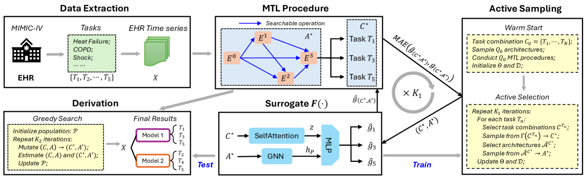
Figure 1. Overview of the proposed AutoDP

3. Methodology

3.1. Preliminaries

3.1.1. Problem definition

Assume we have the input EHR data for multiple patients where each patient is represented as $\mathbf{X}\in\mathbb{R}^{L\times d_{e}}$, where $L$ is the time sequence length and $d_{e}$ is the hidden dimension of the input features. And for each patient, we have totally $N$ prediction tasks conditioned on the EHR data, denoted as $\mathcal{T}=\{T_{1},T_{2},\cdots,T_{N}\}$. Our goal is to maximize the overall MTL performance gain for all these prediction tasks compared to single task training.

First, we make formal definition of MTL gain. We first conduct single task training on each task independently using a specific backbone model (such as RNN), and obtain the single-task performance for all tasks in terms of a predefined metric (such as averaged precision), denoted as $\{s_{1},s_{2},\cdots,s_{N}\}$. Then, the MTL gain is defined as:

(1) $$g_{i}=\frac{(m_{i}-s_{i})}{s_{i}},i=1,\cdots,N,$$

where $m_{i}$ is the multi-task performance for $T_{i}$. Therefore, our objective is to maximize the overall gain for all tasks: $G=\frac{1}{N}\sum_{i=1}^{N}g_{i}$.

In order to achieve that, our proposed method solves two searching problems at the same time using AutoML. First, we search for a list of task combinations that defines which tasks should be trained together. Second, we determine the optimal model architecture for each task combination. We aim at finding the optimal configuration for both, such that the highest overall gain $G$ is attained.

3.1.2. Task grouping search space

Given $N$ tasks, we can have totally $2^{N}-1$ task combinations, denoted as $\mathcal{C}=\{C_{1},C_{2},\cdots,C_{2^{N}-1}\}$, where every $C$ is a subset of $\mathcal{T}$. Given a budget $B$, we aim at searching for maximally $B$ task combinations from $\mathcal{C}$ to determine which tasks should be trained together such that the task combinations should cover all $N$ tasks so that we are able to obtain $\{m_{1},m_{2},\cdots,m_{N}\}$. If one task $T_{n}$ appears in multiple task combinations, we simply choose the highest performance for it as $m_{n}$.

3.1.3. Architecture search space

For every task combination, we also need to search for an MTL architecture to model the EHR data. We adopt the hard sharing mechanism as in most existing works (Harutyunyan et al., 2019; Suo et al., 2017), which consists of a shared encoder for extracting the latent representation of the input EHR and multiple task specific classifiers to generate the output for every task.

Specifically, we enable the search for the optimal shared encoder. For the search space of the encoder, we adopt the setting of directed acyclic graph (DAG) (Liu et al., 2019). The architecture is represented as a DAG that consists of $P$ ordered computation nodes, and each node is a latent feature that has connections to all previous nodes. For each connection (also called edge), we can choose one operation from a predefined set of candidate operations $\mathcal{O}$ for feature transformation. Let $\mathbf{E}^{0}=\mathbf{X}$, the formulation of node $p$ is defined as follows:

(2) $$\mathbf{E}^{p}=\sum_{i=0}^{p-1}o_{(i,p)}(\mathbf{E}^{i}),o_{(i,p)}\in\mathcal{O},$$

where node features $\mathbf{E}^{i}\in\mathbb{R}^{L\times d_{e}}$’s all have the same dimension as $\mathbf{X}$, and $o_{(i,p)}$ is the operation that transform $\mathbf{E}^{i}$ to $\mathbf{E}^{p}$. Essentially, sampling one architecture from the search space is equivalent to sampling one operation for every edge in the DAG. In this way, we can get the set of all possible architectures denoted as $\mathcal{A}$.

To make final prediction, we take the last node representation $\mathbf{E}^{P}$ as the encoded feature for the input EHR, and use task specific classifiers to output final predictions, which are all fixed fully connected network layers.

3.1.4. MTL procedure

To evaluate a specific sample from the joint search space $\mathcal{C}\times\mathcal{A}$, we need to conduct an MTL experiment to obtain the multi-task performances. Specifically, given an architecture $A\in\mathcal{A}$ and a task combination $C\in\mathcal{C}$, we train the model $A$ to predict for all tasks in $C$ and get the multi-task performances for those tasks. Then, we can compute their gains by Eq.(1). In this way, we are able to evaluate how much gains that this sample $(C,A)$ could achieve.

3.2. Overview

We propose a surrogate model based AutoML framework to search for the optimal task grouping and corresponding architectures simultaneously. To achieve that, we need to first evaluate the MTL gains for all the samples in the joint search space $\mathcal{C}\times\mathcal{A}$, and then select the best $B$ samples (pairs of task combinations and architectures) that maximize $G$. However, it is not practical to obtain the ground-truth gains for every sample, since the whole search space is normally very huge and every MTL procedure is also considerably expensive. Therefore, we build a neural network (called surrogate model) to learn the mapping from a pair of task combination and architecture to the multi-task gains:

(3) $$\mathbf{g}_{(C,A)}=F(C,A),C\in\mathcal{C},A\in\mathcal{A},$$

where $\mathbf{g}_{(C,A)}\in\mathbb{R}^{|C|}$ is the per-task gains for task combination $C\in\mathcal{C}$ if using $A$ as the model, and $F(\cdot)$ is the surrogate model. In this way, we only need to evaluate the ground truth gains for a small subset of samples from the search space, and use them to train the surrogate model for estimating all other unseen samples. The assumption is that the multi-task gains are essentially determined by the configuration of the task combination and the architecture, so there exists an underlying mapping that could be learned by a neural network. We set universal hyperparameters and optimization settings for all MTL procedures, hence the influence of other factors can be ignored.

Specifically, we introduce the model architecture of the surrogate model in Section 3.3. Then, we outline the training procedure of the surrogate model in Section 3.4, where we propose an active learning strategy to collect training samples. Eventually, we use greedy search to derive the final configuration of task grouping and architectures by utilizing the trained surrogate model, as discussed in Section 3.5. The framework overview is shown in Figure 1.

1

Input: Training set $\mathcal{D}$, surrogate model parameter $\mathbf{\Theta}$, $Q_{1}$, $Q_{2}$, $K_{1}$; $Q_{1}>Q_{2}$.

Output: Updated $\mathcal{D}$ and $\mathbf{\Theta}$

2

3for $k=1,2,\cdots,K_{1}$ do

4       for $n=1,2,\cdots,N$ do

5             Collect all task combinations that contains $T_{n}$: $\mathcal{C}^{T_{n}}=\{C_{j}|\forall C_{j}\in\mathcal{C},T_{n}\in C_{j}\}$;

6             for $\forall C_{j}\in\mathcal{C}^{T_{n}}$ do

7                   Randomly sample $Q_{1}$ architectures from $\mathcal{A}$, denote the set as $\mathcal{A}^{C_{j}}$;

8                   Forward the surrogate model to collect gains for $T_{n}$ with every architecture in $\mathcal{A}^{C_{j}}$: $\mathcal{G}=\{\mathbf{g}[T_{n}]|\forall A\in\mathcal{A}^{C_{j}},\mathbf{g}=F(C_{j},A)\}$;

9                   Select the top $Q_{2}$ architectures from $\mathcal{A}^{C_{j}}$ with highest gains in $\mathcal{G}$, denoted as $\hat{\mathcal{A}}^{C_{j}}$;

10                   Calculate the mean over top $Q_{2}$ gains from $\mathcal{G}$, denoted as ${g}^{C_{j}}$;

11                  

12             end for

13            Build the sampling distribution over $\mathcal{C}^{T_{n}}$ as: $\mathbf{\Gamma}(\mathcal{C}^{T_{n}})=\{{\rm exp}({g}^{C_{j}}),\forall C_{j}\in\mathcal{C}^{T_{n}}\}$;

14             Sample a task combination $C^{*}$ from $\mathcal{C}^{T_{n}}$ based on $\mathbf{\Gamma}(\mathcal{C}^{T_{n}})$, and randomly sample an architecture $A^{*}$ from $\hat{\mathcal{A}}^{C^{*}}$;

15             Conduct an MTL procedure on $(C^{*},{A}^{*})$, and collect the ground truth labels $\mathbf{g}_{(C^{*},{A}^{*})}$;

16             Add $(C^{*},{A}^{*},\mathbf{g}_{(C^{*},{A}^{*})})$ to $\mathcal{D}$;

17            

18       end for

19      Update $\mathbf{\Theta}$ by training the surrogate model on $\mathcal{D}$;

20      

21 end for

22

Algorithm 1 Active Sampling

3.3. Surrogate Model

For learning the mapping from an input configuration to the multi-task gains, the surrogate model is required to encode both architectures and task combinations. Also, the model needs to output multi-task gains. Therefore, we design a new surrogate model that consists of two encoders that respectively transform the input architecture and task combination into latent representations. Then, two representations are fused together to predict the multi-task gains.

3.3.1. Architecture Encoding

For encoding a given architecture $A$, we apply a graph encoder (Zhang et al., 2019) that is specifically designed for modeling DAGs, which is suitable for encoding the architectures in our search space. It can sequentially update the hidden states for the $P$ computation nodes in preceding order by aggregating information from all predecessors. For node $p$, we have:

(4) $$\mathbf{h}_{p}={\rm Aggregate}(\mathbf{W}_{0}\cdot\mathbf{h}_{0},\mathbf{W}_{1}\cdot\mathbf{h}_{1},\cdots,\mathbf{W}_{p-1}\cdot\mathbf{h}_{p-1}),$$

where $\mathbf{h}_{0}\in\mathbb{R}^{d_{s}}$ is the input node representation which contains trainable parameters, and $\mathbf{W}\in\mathbb{R}^{d_{s}\times d_{s}}$’s are learnable transition matrices constructed for each operation in $\mathcal{O}$. For every operation in the architecture, we also apply the corresponding $\mathbf{W}$ in our graph encoder. For aggregating all incoming representations, we apply average pooling to obtain the node representation $\mathbf{h}_{p}$. Finally, we use the node representation for the last node $\mathbf{h}_{P}$ as the overall encoding for the input architecture.

3.3.2. Task Combination Encoding

For encoding a given task combination $C$, we use the self attention mechanism (Vaswani et al., 2017) to model the high order interactions among the selected tasks in $C$. Specifically, we randomly initialize the embedding for all $N$ tasks, and for task combination $C$, we have:

(5) $$\mathbf{z}={\rm Pool}({\rm SelfAttention}(\mathbf{u}_{1},\mathbf{u}_{2},\cdots,\mathbf{u}_{|C|})),$$

where $\mathbf{u}\in\mathbb{R}^{d_{s}}$’s are corresponding embeddings for the selected tasks and $\mathbf{z}\in\mathbb{R}^{d_{s}}$ is final representation for task combination $C$. Additionally, we also use average pooling on top of the self attention layers to obatin $\mathbf{z}$.

Eventually, we apply a two layer MLP to fuse both architecture encoding $\mathbf{h}_{P}$ and task combination encoding $\mathbf{z}$, and output the predicted gains for all selected tasks $\hat{\mathbf{g}}_{(C,A)}\in\mathbb{R}^{|C|}$. We use the mean absolute error to supervise the surrogate model as follows:

(6) $$\mathcal{L}(\hat{\mathbf{g}}_{(C,A)},\mathbf{g}_{(C,A)})=||\hat{\mathbf{g}}_{(C,A)}-\mathbf{g}_{(C,A)}||_{1},$$

where $\mathbf{g}_{(C,A)}\in\mathbb{R}^{|C|}$ is the ground truth gains generated by conducting an MTL procedure for $(C,A)$.

3.4. Active Sampling

In order to efficiently train the surrogate model defined in previous section, we develop an active sampling method to collect training samples. That is, our method progressively selects the samples that bring higher predicted gains for each task. In this way, the trained surrogate model is able to better facilitate the final selection of optimal task groupings and architectures, which also also improves the sample efficiency for achieving the expected performance gain.

3.4.1. Warm start

Firstly, we warmup the surrogate model by selecting a small number of samples from the search space. Specifically, we use the task combination that contains all $N$ tasks $C_{0}=\{T_{1},\cdots,T_{n}\}$ and randomly sample $Q_{0}$ architectures from $\mathcal{A}$. Then we conduct $Q_{0}$ MTL procedures to evaluate their transferring gains by training on $C_{0}$. In this way, we collect $Q_{0}$ training samples as the initial training set denoted as $\mathcal{D}$. And, we train the surrogate model on $D$, and denote the model parameters as $\mathbf{\Theta}$.

3.4.2. Active selection

Then, we conduct $K_{1}$ rounds of active sampling. For each round, we iterate through all $N$ tasks. With respect to each task $T_{n}$, we build a distribution $\mathbf{\Gamma}$ over the the set of task combinations that contains $T_{n}$ based on the predicted gains for $T_{n}$. From the distribution, we sample one task combination $C^{*}$ that has a large probability to achieve higher gain for $T_{n}$. Then, we also select one architecture $A^{*}$ with high predicted gain for $T_{n}$ when combined with $C^{*}$. The selection of $C^{*}$ and $A^{*}$ is interdependent, and the details are introduced in Algorithm 1. In this way, we collect one sample $(C^{*},A^{*})$ to update the training set $\mathcal{D}$ with respect to each $T_{n}$. At the end of each round, we also update the surrogate model parameters $\mathbf{\Theta}$ with the updated $\mathcal{D}$. After $K_{1}$ rounds, we are able to obtain a well trained surrogate model for estimating the whole search space.

1

Input: Trained surrogate model $F(\cdot)$, $B$, $V$.

Output: Searched population $\mathcal{P}$.

2 Randomly sample $B$ pairs from $\mathcal{C}\times\mathcal{A}$ to initialize $\mathcal{P}$ ;

3 for $v=1,2,\cdots,V$ do

4       Randomly select one pair $(C,A)$ from $\mathcal{P}$;

5       Mutate $(C,A)$ to $(C^{\prime},A^{\prime})$ by changing one task in $C$ or one operation in $A$, and obtain a new population $\mathcal{P}^{\prime}$;

6       Estimate $\mathcal{P}^{\prime}$ and $\mathcal{P}$ using $F(\cdot)$;

7       Choose the better one: $\mathcal{P}\leftarrow Select(\mathcal{P}^{\prime},\mathcal{P})$ ;

8      

9 end for

Algorithm 2 Greedy Search

3.5. Derivation

We derive the final results using only the trained surrogate model. Because of the huge search space, it is still not practical to use brute force search to get the global optimum. Therefore, we propose to apply a greedy method to search for near-optimal solutions.

Given the budget $B$, we aim at searching for $B$ samples from the search space $\mathcal{C}\times\mathcal{A}$ such that the overall gain $G$ is maximized. We use a greedy algorithm to search for the optimal results as shown in Algorithm 2. Specifically, we first randomly initialize the population $\mathcal{P}$ that contains $B$ pairs of task combinations and architectures. Then, at every iteration, we randomly mutate one pair $(C,A)$ from the population and see whether the overall multi-task gain will increase. If so, we update $\mathcal{P}$ accordingly. After $K_{2}$ iterations, we can obtain a near-optimal solution. In practice, we also apply multiple initial populations to avoid getting stuck on local optima. Although we only get approximate solution, our method can already achieve significant improvement over baselines as shown in Section 4.2.

4. Experiments

4.1. Set Up

4.1.1. Dataset & Tasks

We adopt MIMIC - IV dataset (Johnson et al., 2020) for our experiments, which is a publicly available database sourced from the electronic health record of the Beth Israel Deaconess Medical Center. Specifically, we extract the clinical time series data for the 56,908 ICU stays from the database as our input EHR data, with an average sequence length of 72.9. With respect to each ICU stay, we also extract 25 prediction tasks, including chronic, mixed, and acute care conditions. Each condition is associated with a binary label indicating whether the patient has the corresponding condition during the ICU stay.

To prepare our dataset, we adopt the data pre-processing pipeline outlined in Harutyunyan, et al. (Harutyunyan et al., 2019). Given that the original implementation is designed for MIMIC-III (Johnson et al., 2016), we make specific modifications to tailor it for MIMIC-IV. The 25 labels are defined using the Clinical Classifications Software (CCS) for ICD-9 code. Consequently, we first map the ICD-10 codes in the MIMIC-IV database to ICD-9 codes before generating the labels. After processing, we have the feature dimension $d_{e}$ as 76. We partition the dataset as train, validation and test sets with a ratio of $0.7:0.15:0.15$.

4.1.2. Baselines

To compare the proposed method with existing work, we choose several state-of-art-baselines, including both hand-crafted and automated methods. Specifically, as described below, we include several human-designed EHR encoders to compare with the searched architecture we defined in Eq. (2). Also, we include one NAS method and one multi-task grouping method as the automated baselines. More importantly, we combine the multi-task grouping method with the NAS method and hand-crafted encoders to show the superiority of our joint optimization method.

• EHR encoders: We choose four models that are widely utilized for analyzing EHR time series, including LSTM (Hochreiter and Schmidhuber, 1997), Transformer (Vaswani et al., 2017), Retain (Choi et al., 2016b) and Adacare (Ma et al., 2020).

• NAS: We choose DARTS (Liu et al., 2019) as the NAS baseline, which proposes a differentiable search method for efficient architecture search. We apply it to our search space $\mathcal{A}$ to find better EHR encoders. It has also been adopted for searching better MTL architectures in most state-of-the-art works (Sun et al., 2020; Guo et al., 2020; Gao et al., 2020; Zhang et al., 2022).

• Multi-task grouping: MTG-Net (Song et al., 2022) is the current state-of-the-art multi-task grouping algorithm, which uses a meta learning approach to learn the high-order relationships among different tasks. We refer to this method as MTG in latter sections.

4.1.3. Evaluation Metric

We use two widely used metrics for binary classification to evaluate our method and baselines: ROC (Area Under the Receiver Operating Characteristic curve) and AVP (Averaged Precision). During surrogate model training, we use AVP as the metric to compute multi-task gains as in Eq. (1).

Table 1. Performance of the single task backbone.

Task	ROC	AVP
Acute and unspecified renal failure	0.7827	0.5647
Acute cerebrovascular disease	0.9079	0.4578
Acute myocardial infarction	0.7226	0.1761
Cardiac dysrhythmias	0.6948	0.5168
Chronic kidney disease	0.7296	0.4383
Chronic obstructive pulmonary disease and bronchiectasis	0.6791	0.2689
Complications of surgical procedures or medical care	0.7229	0.4045
Conduction disorders	0.6712	0.1880
Congestive heart failure; nonhypertensive	0.7601	0.5129
Coronary atherosclerosis and other heart disease	0.7351	0.5589
Diabetes mellitus with complications	0.8844	0.5559
Diabetes mellitus without complication	0.7484	0.3355
Disorders of lipid metabolism	0.6730	0.5816
Essential hypertension	0.6298	0.5258
Fluid and electrolyte disorders	0.7396	0.6129
Gastrointestinal hemorrhage	0.7076	0.1281
Hypertension with complications and secondary hypertension	0.7141	0.4243
Other liver diseases	0.6849	0.2303
Other lower respiratory disease	0.6371	0.1417
Other upper respiratory disease	0.7602	0.2228
Pleurisy; pneumothorax; pulmonary collapse	0.7051	0.1417
Pneumonia	0.8171	0.3786
Respiratory failure; insufficiency; arrest (adult)	0.8651	0.5497
Septicemia (except in labor)	0.8291	0.4866
Shock	0.8792	0.5574

Table 2. Hyperparameter setting.

Parameters		Task @ 5	Task @ 10	Task @ 25
# of tasks	$N$	5	10	25
Dimension of $F(\cdot)$	$d_{s}$	32	32	64
# of nodes	$P$	2	2	3
Active sampling	$Q_{0}$	10	10	20
	$Q_{1}$	50	50	50
	$Q_{2}$	5	5	5
	$K_{1}$	15	30	30
Greedy search	$K_{2}$	1000	1000	1000
	$B$	3	5	10
Runtime	GPU Hours	$\thicksim$ 20	$\thicksim$ 75	$\thicksim$ 250

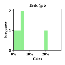
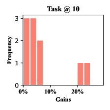
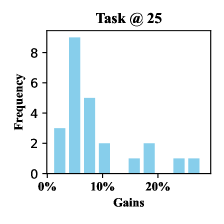
Figure 2. Histogram of task gains for AutoDP in terms of Averaged Precision.

4.1.4. Implementation

We implement the framework using the PyTorch framework and run it on an NVIDIA A100 GPU. Given the dataset we have, we first train a vanilla LSTM for every task independently, and report the backbone performance in Table 1, which can be further used to compute multi-task gains. For, the proposed method, we run three settings of experiments: Task @ 5, Task @ 10 and Task @ 25, which refers to using the first 5 tasks, 10 tasks and 25 tasks respectively. For different settings, we use specific hyperparameters as shown in Table 2. Besides that, we define the candidate operation set $\mathcal{O}$ as {Identity, Zero, FFN, RNN , Attention}, which includes widely used operations for processing EHR time series. Among them, Identity means maintaining the output identical to the input. Zero means setting all the values of the input feature to 0. Attention and FFN represents one self-attention layer and one feed-forward layer respectively, which are the same as in Transformer (Vaswani et al., 2017). RNN is one recurrent layer, and we adopt LSTM (Hochreiter and Schmidhuber, 1997) in our framework. For all the MTL procedures and baseline training, we apply the batch size of 64 and learning rate of $3e-4$. For training the surrogate model, we use the batch size of 5 and learning rate of $5e-5$. During searching, we compute all multi-task gains on the validation set for guiding the surrogate model training. After we obtain the optimal configuration, we train the searched models and report their multi-task gains on the test set.

Table 3. Performance comparison in terms of averaged per-task gain over single task backbone (All results are in the form of percentage values %).

Task Groups	Tasks @ 5		Tasks @ 10		Tasks @ 25
Metric	ROC	AVP	ROC	AVP	ROC	AVP
LSTM	+0.09	+0.18	+1.06	+3.22	+1.83	+7.46
Transformer	+0.97	+4.82	+1.41	+4.14	+1.75	+7.45
Retain	+0.46	+1.80	+0.66	+0.75	+1.41	+5.88
Adacare	+1.03	+5.21	+1.32	+4.05	+1.68	+6.94
DARTS	+1.28	+5.01	+2.01	+6.87	+1.87	+7.71
MTG+LSTM	+0.51	+2.10	+0.65	1.87	+1.74	+7.40
MTG+Transformer	+0.91	+3.64	+1.20	+3.95	+1.79	+9.15
MTG+Retain	+0.55	+3.11	+1.51	+5.20	+1.54	+8.87
MTG+Adacare	+1.25	+5.78	+1.44	+4.63	+1.75	+7.84
MTG+DARTS	+1.47	+6.41	+2.02	+6.65	+2.41	+11.76
AutoDP	+1.49	+7.12	+2.08	+7.53	+2.68	+12.70

4.2. Performance Evaluation

We compare our method with various baselines and show the results in Table 3. Our method can outperform the baselines at all three settings in terms of averaged per-task gain for ROC and AVP, which is a significant improvement over existing MTL frameworks for EHR data.

First, without considering task grouping, we train one shared model to predict for all tasks in three settings and compute the multi-task gain for them. For the hand-crafted encoders, they can only bring minimal average performance gain over single-task backbones, especially for Task @ 5. Note that even if the average per-task gain is positive, there is a great chance for some tasks to have negative gains. Also, we apply DARTS to the architecture search space we defined $\mathcal{A}$ for each setting and use the searched encoder to predict for all tasks. We can observe that the searched architectures generally perform better than hand-crafted models, but might get worse results in some rare cases. Without the task grouping, it is difficult to achieve higher performance gains even for searched architectures. This means naively putting all tasks together to train will not provide much improvement over single task training.

Moreover, we combine all the encoders with the multi-task grouping baseline to achieve better results. Specifically, we first run the MTG method to perform task grouping under the same budgets with our method as defined in Table 2. For each task group, we employ all four EHR encoders and the DARTS search algorithm. The results show that the sequential optimization over task grouping and architecture search (MTG+DARTS) performs better than other hand-crafted encoders. Compared to the best baseline, our method is able to achieve higher gains at all three setting. We attribute this to the superiority of joint optimization over task grouping and architecture search, which can potentially find global optimal configurations for both aspects.

Beside the overall performance gain, we also look at the distribution of performance gains for each individual task as shown in Figure 2. We can observe that the proposed method does not have the issue of negative transfer, since all tasks have a positive gain. Also, for some of the tasks, it can achieve over $20\%$ improvement, which further shows the effectiveness of AutoDP.

4.3. Hyperparameter Analysis

Here, we analyze the effect of two vital hyperparameters of our method: $K_{1}$ and $B$. We try out different values of them under the setting of Task @ 25 and report the corresponding averaged per-task gain of AVP in Figure 3.

First, $K_{1}$ determines the number of training samples collected during searching. Given that each sample involves an MTL procedure, it constitutes a major portion of the computation cost. Therefore, our goal is to find an optimal value for $K_{1}$, striking a balance between cost-effectiveness and achieving commendable performance. Examining the left figure, we observe a direct correlation between the increase of $K_{1}$ and a corresponding improvement in performance. This relationship is obvious, as more rounds lead to more training data for the surrogate model. Furthermore, we notice that the performance change become less pronounced after $K_{1}$ reaches 25. This suggests that the surrogate model effectively learns the distribution of the search space after consuming $25\times 25$ training samples during active selection (25 samples per round). As a result, we can empirically decide to halt the iteration at this point with little impact on performance.

Second, $B$ determines the number of task groups for the final configuration, which indicates the number of MTL models needed for achieving the expected performance gain after searching. We also observe similar phenomenon that the performance becomes stable after $B$ reaches certain amount. We could also choose the optimal value for $B$ accordingly.

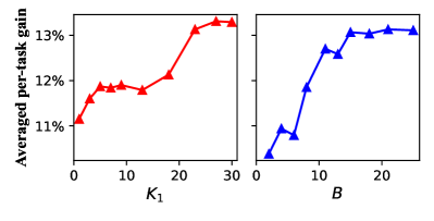
Figure 3. Analysis for the number of active sampling rounds $K_{1}$ and the budget of task groups $B$ under the setting of Task @ 25.

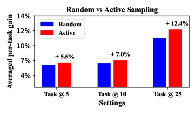
Figure 4. Comparing the proposed active sampling strategy with random sampling.

4.4. Random vs Active Sampling

We further analyze the effect of the proposed active sampling strategy. In order to demonstrate its effectiveness, we conduct a comparative analysis with the random sampling method. In the case of the random method, an equivalent number of training samples is randomly selected from the search space to train the surrogate model. Then, the trained surrogate model is employed for deriving the final configuration in same way as introduced in Section 3.5. Finally, we compare the averaged per-task gain of AVP achieved by each approach, which are shown in Figure 4.

Under all three settings, the proposed active sampling strategy is able to achieve significant improvement over random baseline, ranging from $5.48\%$ to $12.39\%$. It is noteworthy that active sampling tends to have larger improvement when the number of tasks grows. We attribute this to the expansion of the search space. By progressively selecting samples capable of yielding higher performance gains during searching, the active sampling method has superior sample efficiency than the random method. Therefore, in the case of Task @ 25, where the fraction of samples with ground-truth evaluations is exceptionally small (approximately $2e-5\%$), the active sampling method can achieve larger improvement over random method.

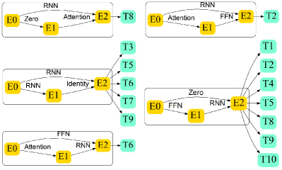
Figure 5. Illustration of the searched configuration under the setting of Task @ 10.

4.5. Visualization of the Searched Configurations

Here, we show one example of the final configuration for setting Task @ 10 in Figure 5. The proposed AutoDP identifies 5 different task groups and also searches for the corresponding architectures. We can observe that some of the tasks tend to be trained independently, while others are grouped together for joint training. This supports our claim that fine-grained task grouping is necessary to bring the optimal performance gain. Also, the optimal architecture is also different for each task group, which further justifies the necessity of joint optimization over task grouping and architecture search.

5. Conclusions

In this paper, we propose AutoDP, an automated multi-task learning framework for joint disease prediction on EHR data. Compared to existing work, our method largely improves the design of task grouping and model architectures by reducing human interventions. Experimental results on real-world EHR data demonstrate that the proposed framework not only outperforms existing state-of-the-art methods, but also maintains a feasible search cost. In future work, we will try to enable the searching for more aspects of MTL, such as hyperparameters, optimization methods, etc.

References

- (1)
- Ahn et al. (2019) Chanho Ahn, Eunwoo Kim, and Songhwai Oh. 2019. Deep elastic networks with model selection for multi-task learning. In Proceedings of the IEEE/CVF international conference on computer vision. 6529–6538.
- Bragman et al. (2019) Felix JS Bragman, Ryutaro Tanno, Sebastien Ourselin, Daniel C Alexander, and Jorge Cardoso. 2019. Stochastic filter groups for multi-task cnns: Learning specialist and generalist convolution kernels. In Proceedings of the IEEE/CVF International Conference on Computer Vision. 1385–1394.
- Choi et al. (2016a) Edward Choi, Mohammad Taha Bahadori, Andy Schuetz, Walter F Stewart, and Jimeng Sun. 2016a. Doctor ai: Predicting clinical events via recurrent neural networks. In Machine learning for healthcare conference. PMLR, 301–318.
- Choi et al. (2016b) Edward Choi, Mohammad Taha Bahadori, Jimeng Sun, Joshua Kulas, Andy Schuetz, and Walter Stewart. 2016b. Retain: An interpretable predictive model for healthcare using reverse time attention mechanism. In Advances in Neural Information Processing Systems. 3504–3512.
- Elsken et al. (2019) Thomas Elsken, Jan Hendrik Metzen, and Frank Hutter. 2019. Neural architecture search: A survey. The Journal of Machine Learning Research 20, 1 (2019), 1997–2017.
- Fifty et al. (2021) Chris Fifty, Ehsan Amid, Zhe Zhao, Tianhe Yu, Rohan Anil, and Chelsea Finn. 2021. Efficiently identifying task groupings for multi-task learning. Advances in Neural Information Processing Systems 34 (2021), 27503–27516.
- Gao et al. (2020) Yuan Gao, Haoping Bai, Zequn Jie, Jiayi Ma, Kui Jia, and Wei Liu. 2020. Mtl-nas: Task-agnostic neural architecture search towards general-purpose multi-task learning. In Proceedings of the IEEE/CVF Conference on computer vision and pattern recognition. 11543–11552.
- Guo et al. (2020) Pengsheng Guo, Chen-Yu Lee, and Daniel Ulbricht. 2020. Learning to branch for multi-task learning. In International conference on machine learning. PMLR, 3854–3863.
- Harutyunyan et al. (2019) Hrayr Harutyunyan, Hrant Khachatrian, David C Kale, Greg Ver Steeg, and Aram Galstyan. 2019. Multitask learning and benchmarking with clinical time series data. Scientific data 6, 1 (2019), 96.
- He et al. (2016) Kaiming He, Xiangyu Zhang, Shaoqing Ren, and Jian Sun. 2016. Deep residual learning for image recognition. In Proceedings of the IEEE conference on computer vision and pattern recognition. 770–778.
- He et al. (2021) Xin He, Kaiyong Zhao, and Xiaowen Chu. 2021. AutoML: A survey of the state-of-the-art. Knowledge-Based Systems 212 (2021), 106622.
- Hochreiter and Schmidhuber (1997) Sepp Hochreiter and Jürgen Schmidhuber. 1997. Long short-term memory. Neural computation 9, 8 (1997), 1735–1780.
- Huang et al. (2019) Kexin Huang, Jaan Altosaar, and Rajesh Ranganath. 2019. Clinicalbert: Modeling clinical notes and predicting hospital readmission. arXiv preprint arXiv:1904.05342 (2019).
- Johnson et al. (2020) Alistair Johnson, Lucas Bulgarelli, Tom Pollard, Steven Horng, Leo Anthony Celi, and Roger Mark. 2020. Mimic-iv. PhysioNet. Available online at: https://physionet. org/content/mimiciv/1.0/(accessed August 23, 2021) (2020).
- Johnson et al. (2016) Alistair EW Johnson, Tom J Pollard, Lu Shen, Li-wei H Lehman, Mengling Feng, Mohammad Ghassemi, Benjamin Moody, Peter Szolovits, Leo Anthony Celi, and Roger G Mark. 2016. MIMIC-III, a freely accessible critical care database. Scientific data 3, 1 (2016), 1–9.
- Liu et al. (2019) Hanxiao Liu, Karen Simonyan, and Yiming Yang. 2019. DARTS: Differentiable Architecture Search. In International Conference on Learning Representations.
- Liu et al. (2022) Shiqing Liu, Haoyu Zhang, and Yaochu Jin. 2022. A survey on surrogate-assisted efficient neural architecture search. arXiv preprint arXiv:2206.01520 (2022).
- Ma et al. (2017) Fenglong Ma, Radha Chitta, Jing Zhou, Quanzeng You, Tong Sun, and Jing Gao. 2017. Dipole: Diagnosis prediction in healthcare via attention-based bidirectional recurrent neural networks. In Proceedings of the 23rd ACM SIGKDD international conference on knowledge discovery and data mining. 1903–1911.
- Ma et al. (2021) Fenglong Ma, Muchao Ye, Junyu Luo, Cao Xiao, and Jimeng Sun. 2021. Advances in Mining Heterogeneous Healthcare Data. In Proceedings of the 27th ACM SIGKDD Conference on Knowledge Discovery & Data Mining. 4050–4051.
- Ma et al. (2020) Liantao Ma, Junyi Gao, Yasha Wang, Chaohe Zhang, Jiangtao Wang, Wenjie Ruan, Wen Tang, Xin Gao, and Xinyu Ma. 2020. AdaCare: Explainable Clinical Health Status Representation Learning via Scale-Adaptive Feature Extraction and Recalibration. In AAAI.
- Razavian et al. (2016) Narges Razavian, Jake Marcus, and David Sontag. 2016. Multi-task prediction of disease onsets from longitudinal laboratory tests. In Machine learning for healthcare conference. PMLR, 73–100.
- Real et al. (2019) Esteban Real, Alok Aggarwal, Yanping Huang, and Quoc V Le. 2019. Regularized evolution for image classifier architecture search. In Proceedings of the aaai conference on artificial intelligence, Vol. 33. 4780–4789.
- Song et al. (2022) Xiaozhuang Song, Shun Zheng, Wei Cao, James Yu, and Jiang Bian. 2022. Efficient and effective multi-task grouping via meta learning on task combinations. Advances in Neural Information Processing Systems 35 (2022), 37647–37659.
- Standley et al. (2020) Trevor Standley, Amir Zamir, Dawn Chen, Leonidas Guibas, Jitendra Malik, and Silvio Savarese. 2020. Which tasks should be learned together in multi-task learning?. In International Conference on Machine Learning. PMLR, 9120–9132.
- Sun et al. (2020) Ximeng Sun, Rameswar Panda, Rogerio Feris, and Kate Saenko. 2020. Adashare: Learning what to share for efficient deep multi-task learning. Advances in Neural Information Processing Systems 33 (2020), 8728–8740.
- Suo et al. (2017) Qiuling Suo, Fenglong Ma, Giovanni Canino, Jing Gao, Aidong Zhang, Pierangelo Veltri, and Gnasso Agostino. 2017. A multi-task framework for monitoring health conditions via attention-based recurrent neural networks. In AMIA annual symposium proceedings, Vol. 2017. American Medical Informatics Association, 1665.
- Vaswani et al. (2017) Ashish Vaswani, Noam Shazeer, Niki Parmar, Jakob Uszkoreit, Llion Jones, Aidan N Gomez, Łukasz Kaiser, and Illia Polosukhin. 2017. Attention is all you need. In Advances in neural information processing systems. 5998–6008.
- Wang et al. (2014) Xiang Wang, Fei Wang, Jianying Hu, and Robert Sorrentino. 2014. Exploring joint disease risk prediction. In AMIA annual symposium proceedings, Vol. 2014. American Medical Informatics Association, 1180.
- Waring et al. (2020) Jonathan Waring, Charlotta Lindvall, and Renato Umeton. 2020. Automated machine learning: Review of the state-of-the-art and opportunities for healthcare. Artificial intelligence in medicine 104 (2020), 101822.
- Xu et al. (2019) Enliang Xu, Shiwan Zhao, Jing Mei, Eryu Xia, Yiqin Yu, and Songfang Huang. 2019. Multiple MACE risk prediction using multi-task recurrent neural network with attention. In 2019 IEEE International Conference on Healthcare Informatics (ICHI). IEEE, 1–2.
- Zhang et al. (2022) Lijun Zhang, Xiao Liu, and Hui Guan. 2022. Automtl: A programming framework for automating efficient multi-task learning. Advances in Neural Information Processing Systems 35 (2022), 34216–34228.
- Zhang et al. (2019) Muhan Zhang, Shali Jiang, Zhicheng Cui, Roman Garnett, and Yixin Chen. 2019. D-vae: A variational autoencoder for directed acyclic graphs. Advances in Neural Information Processing Systems 32 (2019).
- Zhao et al. (2022) Xiongjun Zhao, Xiang Wang, Fenglei Yu, Jiandong Shang, and Shaoliang Peng. 2022. UniMed: Multimodal Multitask Learning for Medical Predictions. In 2022 IEEE International Conference on Bioinformatics and Biomedicine (BIBM). IEEE, 1399–1404.
- Zoph and Le (2016) Barret Zoph and Quoc V Le. 2016. Neural architecture search with reinforcement learning. arXiv preprint arXiv:1611.01578 (2016).
- Zoph et al. (2018) Barret Zoph, Vijay Vasudevan, Jonathon Shlens, and Quoc V Le. 2018. Learning transferable architectures for scalable image recognition. In Proceedings of the IEEE conference on computer vision and pattern recognition. 8697–8710.