Density and Affinity Dependent Social Segregation and Arbitrage Equilibrium in a Multi-class Schelling Game
Abstract
Contrary to the widely believed hypothesis that larger, denser cities promote socioeconomic mixing, a recent study [1] reports the opposite behavior, i.e. more segregation. Here, we present a game-theoretic model that predicts such a density-dependent segregation outcome in both one- and two-class systems. The model provides key insights into the analytical conditions that lead to such behavior. Furthermore, the arbitrage equilibrium outcome implies the equality of effective utilities among all agents. This could be interpreted as all agents being equally ”happy” in their respective environments in our ideal society. We believe that our model contributes towards a deeper mathematical understanding of social dynamics and behavior, which is important as we strive to develop more harmonious societies.
I Introduction
The increasing economic inequality and the related increase in socioeconomic segregation are of concern in many societies. In the U.S., for example, this segregation leads to wide variations in lifestyles and life outcomes. This lack of mixing and social interactions across the socioeconomic spectrum contributes to social tensions and political polarization. It is generally believed that in large, dense, urbanized environments, the diverse happenstance of social interactions among people leads to more mixing and less segregation. However, in a recent study, Nilforoshan et al.[1] report that large cities increase rather than reduce socioeconomic segregation, as they can offer a greater choice of differentiated spaces aimed at specific socioeconomic groups. They observe that ”The consistent result that larger, denser cities are more segregated runs counter to the hypothesis that such cities promote socioeconomic mixing by attracting diverse individuals and constraining space in ways that oblige them to encounter one
other. Our results support the opposite hypothesis: big cities allow their inhabitants to seek out people who are more like themselves.”
In this work, we present a mathematical model and its agent-based simulation that demonstrate this density-dependent segregation outcome. Our work is related to Schelling’s seminal game-theoretic model of social segregation[2]. It is an agent-based model in which agents move according to a specified utility function that depends on their neighbors. He showed that although agents may only have a mild preference, they still choose to segregate into neighborhoods of similar individuals over time. Schelling’s model was originally proposed to study social segregation phenomena but can also be related to phase separation in chemistry and physics [3, 4, 5, 6, 7]. Hence, in this paper, we use the terms phase separation and social segregation interchangeably.
It turns out that this connection between two apparently very different domains, sociology/economics and physics/chemistry, is not just coincidental. There exists a deep connection between game theory (the mathematical framework for modeling phenomena in sociology/economics) and statistical mechanics (the mathematical framework for modeling equilibrium phenomena in physics/chemistry) that was identified by Venkatasubramanian [8]. Inspired by this insight, he developed a novel analytical framework, called statistical teleodynamics, which is a synthesis of the central concepts and techniques of statistical mechanics and population game theory [9, 8, 10]. In this paper, we use this framework to model the dynamics of socioeconomic segregation, which reveals interesting insights. We study Schelling-like systems with one-class and two-class models to determine the analytical conditions under which they would undergo socioeconomic segregation. We extend the analysis first introduced by Venkatasubramanian et al.[10] to two-class systems and a wider range of parameters.
II Mathematical Formulation: Pursuit of Maximum Utility and Arbitrage Equilibrium
Our goal is to understand the fundamental principles and mechanisms of self-organization of goal-driven social agents. Toward that end, we develop simple models that offer an appropriate coarse-grained description of the system. Unlike atoms and molecules, social agents do not behave precisely and predictably. Therefore, we have deliberately tried to keep the models as simple as possible and not be restricted by system-specific details and nuances without losing key insights and relevance to empirical phenomena [10].
We also wish to stress that the spirit of our modeling is similar to that of the ideal gas or the Ising model in statistical thermodynamics. Just as real molecules are not point-like objects or are devoid of intermolecular interactions, as assumed in the ideal gas model in statistical mechanics, we make similar simplifying assumptions about the social agents in our model. These can be relaxed to make them more realistic in subsequent refinements like, for example, van der Walls did in thermodynamics. Ideal versions serve as useful starting points and reference states for developing more comprehensive models of self-organization in sociological systems.
The central theme in our theory is that goal-driven social agents constantly pursue maximum utility by jockeying for better positions via self-organization. So, we formulate the problem by first defining the effective utility, , for an agent in state . The effective utility is the net sum of the benefits minus the costs for the agents. Social agents constantly make benefit-cost trade-offs in their self-driven dynamical behavior to improve their socioeconomic fitness, i.e. the effective utility. This results in a delicate dynamic balance of the benefits of aggregation versus the costs of overcrowding the agents. In other words, the benefits of cooperation are balanced with the costs of competition.
Furthermore, driven by natural instincts, agents also balance two competing strategies - exploitation and exploration. Exploitation takes advantage of the opportunities in the immediate, local neighborhood. On the other hand, exploration examines possibilities outside.
We believe that this combination of two main strategies, namely, the benefit-cost trade-offs of the cooperation-competition strategy with an exploitation-exploration strategy, is a fundamental and universal evolutionary mechanism found in most living systems.
We motivate our model by initially considering a one-class system, which is simpler to start with. Here, all agents belong to the same socioeconomic category. As is generally done in Schelling games, we also model the space where the agents operate as a large lattice of local neighborhoods or blocks, each with sites that agents can occupy. There are such blocks, sites, and a total of agents, with an average agent density of . The state of an agent is defined by specifying the block in which it is located, and the state of the system is defined by specifying the number of agents, , in block , for all blocks (). The density of the agents block is given by . Let block also have vacant sites, so . This approach is an extension of our recent model developed for a Schelling-like game scenario [10].
We further formulate the problem by defining the effective utility, , for the one-class agents in block , which agents try to maximize by moving to better locations (i.e., other blocks), if possible. The effective utility is the net sum of the benefits minus the costs and has four components. The first is that an agent prefers to have more agents in its neighborhood, as this aggregation improves its socioeconomic quality of life. Therefore, this affinity benefit term, representing cooperation among agents, is proportional to the number of agents in its neighborhood. We model this as , where is a parameter.
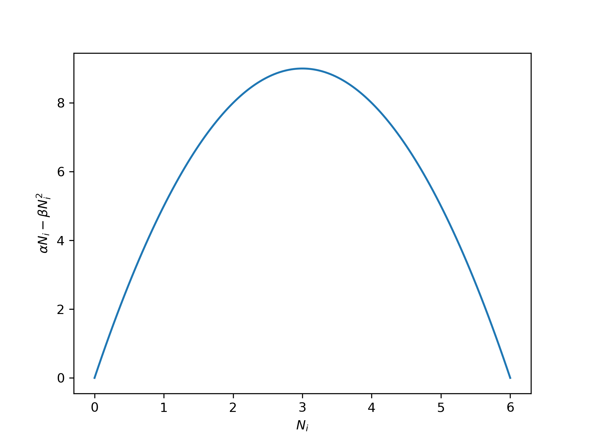
However, this affinity benefit comes with a cost. As more and more agents aggregate, this overcrowding results in a congestion cost term. As Venkatasubramanian explains [8], the resulting net benefit (= benefit - cost) function has an inverted U-like profile (see Fig. 1). This profile is found in many net benefit vs. resource relationships in the real world. As one consumes a resource, it initially leads to increasing net benefit; but after a point, the cost of the resource goes up more quickly than the benefit, thus resulting in decreasing net benefit. The simplest model of this is a quadratic function, , with the quadratic term () modeling the congestion cost.
Regarding exploration, agents derive a benefit by having a large number of vacant sites to potentially move to in the future should such a need arise. This is the instinct to explore other opportunities, as new vacant sites are potentially new sources of socioeconomic benefits. We call this the option benefit term, as agents have the option to move elsewhere if needed. Again, following Venkatasubramanian [8, 11, 10], we model this as , . The logarithmic function captures the diminishing utility of this option, a commonly used feature in economics and game theory. As before, this benefit is also associated with a cost as a result of competition among agents for these vacant sites. We model this disutility of competition as , [9, 8, 11].
Combining these four components, we have the following effective utility function for the agents in block as,
| (1) |
Intuitively, the first two terms in the equation model the benefit-cost trade-off in the exploitation behavior, while the last two model a similar trade-off in exploration.
We can set without any loss of generality. In addition, we set to gain analytical simplicity, but this can be relaxed later if necessary. So we now have
| (2) |
Rewriting this in terms of the density () of agents in block , , and absorbing the constant into and , we have
| (3) |
For simplicity, we define . Therefore, the potential becomes
One can generalize the discrete formulation to a continuous one by replacing by , where the density is a continuous function of radius of the neighborhood as demonstrated by Sivaram and Venkatasubramanian [12] in the self-organized flocking behavior of birds.
Now, according to the theory of potential games [13], an arbitrage equilibrium is reached when the potential is maximized. We can determine the equilibrium utility, , by maximizing the potential (see [8]), but there exists a simpler alternative that is more convenient for our purposes here. To analyze the equilibrium behavior, we can take the simpler agent-based perspective and exploit the fact that at equilibrium, all agents have the same effective utility, i.e. , for all . In other words,
| (5) |
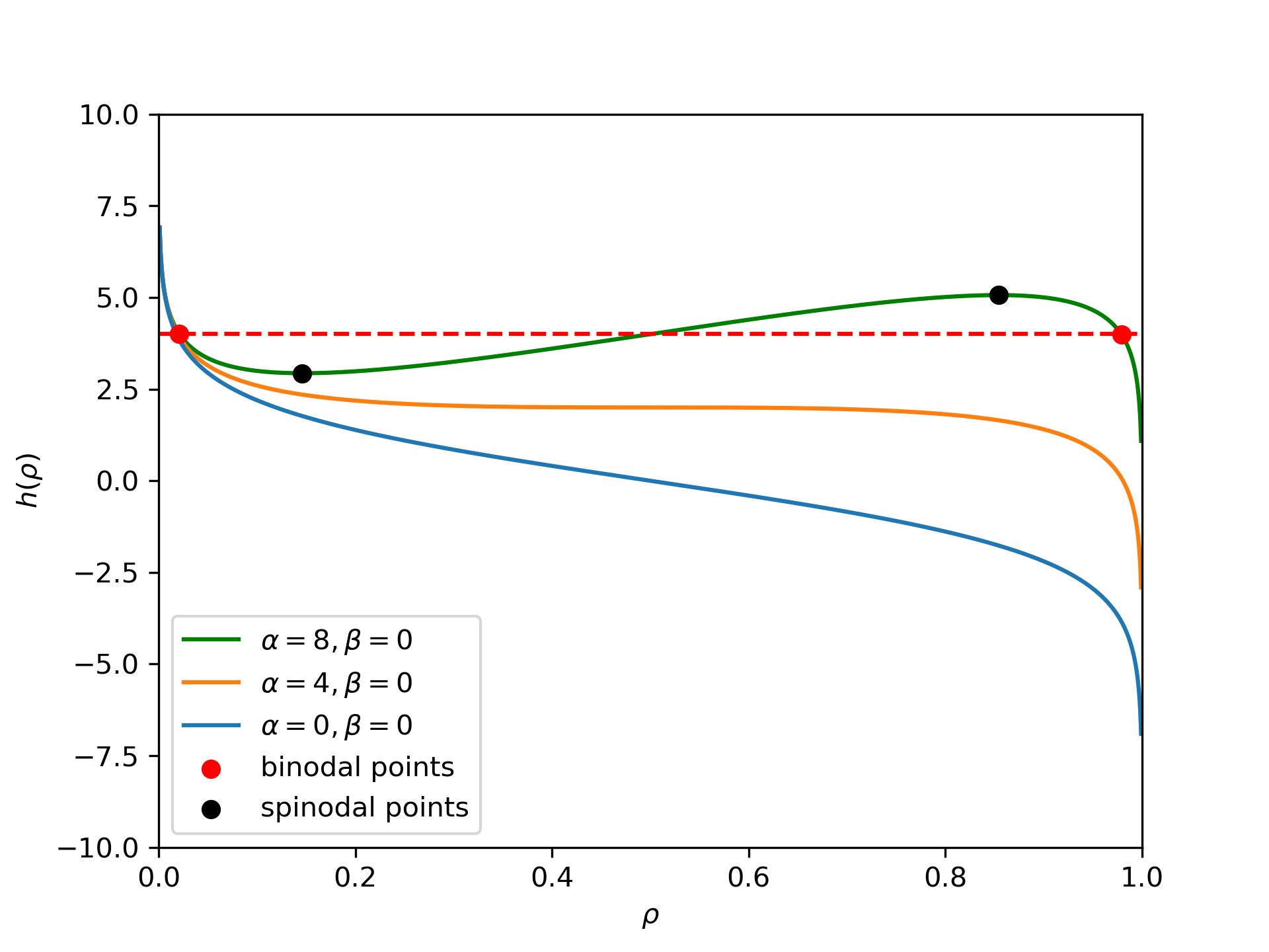
We explore numerically the behavior of as a function of in (5), as shown in Fig. 2 ( , different ). Below a threshold value of and , the utility function is monotonic and has a unique density (blue curve) for a given utility value. Above the threshold, the utility is non-monotonic (green curve) and can have multiple density values for the same utility. The red dotted line shows this. The orange curve is the threshold behavior.
Note that whether all agents remain in a single phase of uniform density dispersed throughout the region or separate into various groups is determined by the slope , which is the second derivative of , . This behavior is mathematically equivalent to spinodal decomposition in thermodynamics, widely studied, for example, in the phase separation of alloys and polymer blends [14, 15].
Although the mathematics of spinodal decomposition is equivalent to the segregation of social agents, there are significant differences in the mechanism of phase separation. In spinodal decomposition in a binary alloy formed with atoms of two metals, say and , spinodal decomposition occurs when the change in free energy during the formation of bonds is less than that of the formation of bonds. However, our utility formulation allows phase separation even in systems with one-class agents. This is because our formulation introduces a disutility due to crowding and competition. These factors encourage agents to be part of large groups. The same behavior is also exhibited by systems with multiclass agents.
In thermodynamics, the phase between the spinodal points (discussed in Appendix A in more detail) is unstable as it corresponds to increasing the free energy of the system, and hence the single phase splits into two phases of different densities to lower the free energy. For the same reason, the phases between the spinodal and binodal points are metastable, and the phases at the binodal points are stable. A similar behavior happens here in statistical teleodynamics as well (see Appendix A).
III Social Segregation in the one-class system: Parametric Regimes
In this section, we determine the parametric regime in which social segregation occurs. To have social segregation in one-class systems, the utility curve should be non-monotonic in nature; more specifically, it should have a minimum and a maximum, as shown in Figure 2. Differentiating Eq.(3) we get
| (6) |
We know that the condition to have minimum or maximum is . To have a minimum and a maximum, there should be two distinct real solutions for in the domain .
| (7) |
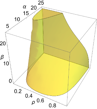
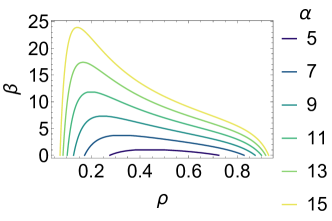
This cubic equation can be solved numerically or using the Cardano formula. One can search in the - space for values that produce two real roots for Eq.(7) in the domain . Fig. 3, shows the -- region (shaded in yellow) within which phase separation occurs. In Fig. 4, we show the 2-D slices of the yellow region of spontaneous phase separation. For a given value of , , and , they show the loci of the two densities (i.e., the low and high density groups) of the corresponding equilibrium states of agents.
IV Agent-based simulations: One-class system
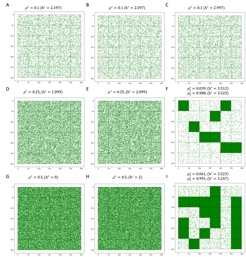
Agent-based simulations were performed for the parameters shown in Figure 2. From the theory we had discussed earlier, we cannot expect phase separation to occur for and . However, phase separation can occur for and when the initial average density is within the spinodal densities. Our agent-based simulations agree with this theoretical prediction.
The equilibrium configuration of the agents for nine sets of simulations is shown in Figure 5. The configurations shown in each row of Figure 5 are for a constant density, and those shown in each column are for the same set of and . As expected, for (configurations A, D, and G) and (configurations B, E, and H), there is no phase separation at any densities. For , phase separation does not occur for (configuration C) because this density is outside the range of spontaneous decomposition.
However, at higher densities (configurations F and I), phase separation occurs because the densities are now within the spinodal region (the yellow region in Fig. 3). In addition, note that the utility of both phases is equal (see Fig. 5 captions). Similar behavior was observed in cases where we kept constant and varied .
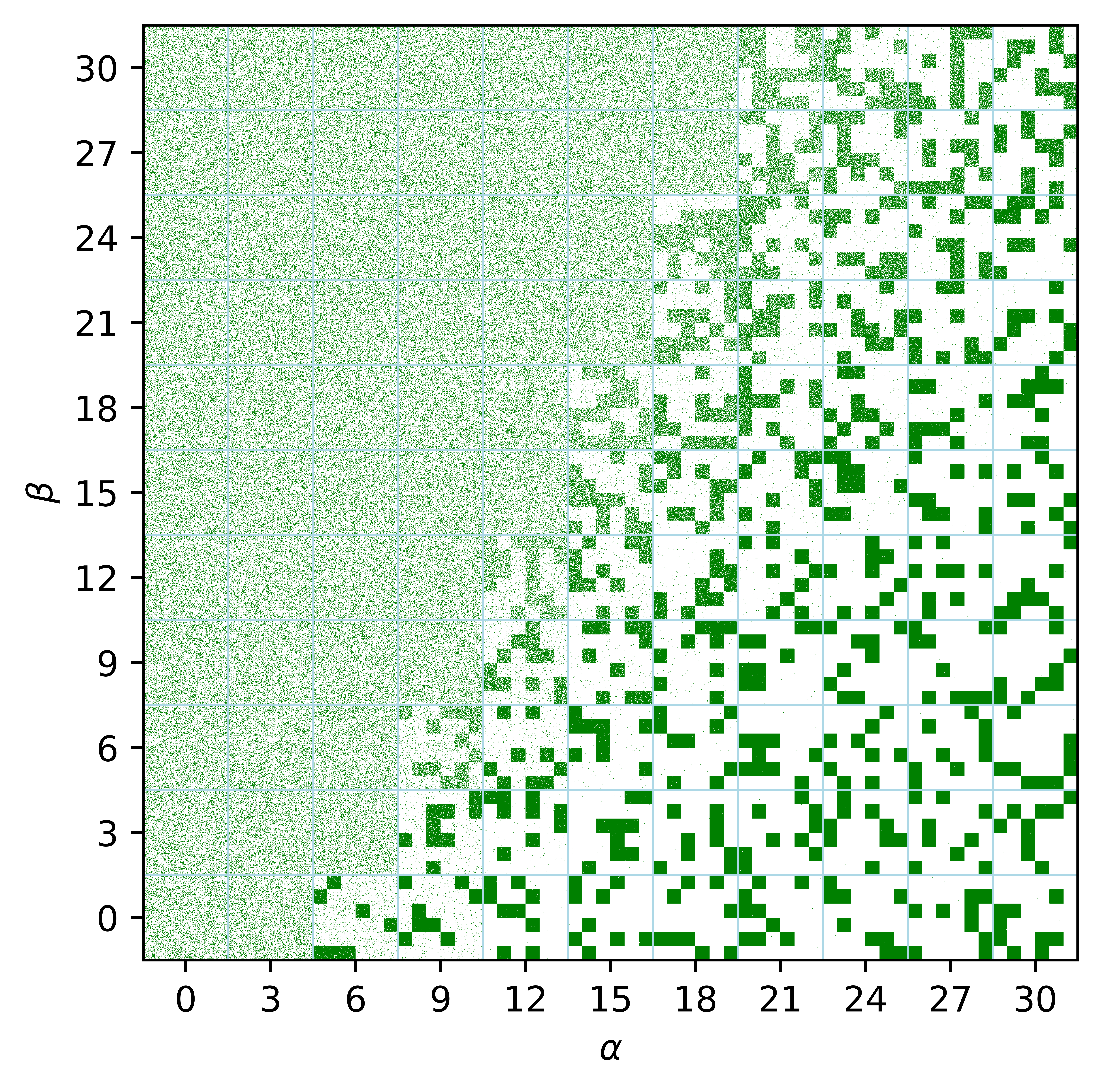
The parameter regime in which phase separation occurs was theoretically predicted and plotted in Figure 3. Our numerical simulations agree with the theoretical predictions. The equilibrium agent configurations for a range of - values are shown in Figure 6. The and coordinates of each configuration indicate the values and used in the simulation.
At low values of , there is no phase separation (for any , see the uniform green region in Figure 6) because there is not much incentive to socially aggregate. However, this changes as increases, because the benefit of aggregation increases (see Eq. 3). So, social segregation occurs spontaneously, and the space divides itself into low-density (white squares) and high-density (green squares) blocks.
This behavior can also be explained by the monotonicity of the curve. At low values of and high values of , the curve is monotonically decreasing. For any fixed , larger values of result in nonmonotonic behavior for the curve. Similarly, for any fixed (), small values of lead to the non-monotonic behavior of the curve. This behavior can be observed in Figure 6. All the simulations shown in Figure 6 are performed for N=22,500.
V Segregation in a Two-class system: Mathematical Analysis
The formulation of a one-class system can readily be generalized to multiclass systems. Here, we discuss a two-class system, as an example, by modifying the vacancy terms in Eq. (2). Consider a class of agents identified as green agents and another class of agents identified as red agents. Their utilities can be defined as follows.
| (8) | |||||
| (9) | |||||
The utilities can be rewritten in terms of densities of the two classes, and , as
| (10) | |||||
| (11) | |||||
where , , , , , and . (Refer to the supplementary material for the derivation.)
For one-class systems, we showed that phase separation occurs when the utility-density curve is nonmonotonic. For two-class systems, the utility of a class depends not only on its density, but also on the density of the other class as well. The utility of each class in a two-class system is shown in Figure 7A. and result in a nonconcave potential function. The nonconcavity of the potential is the primary requirement for phase separation. The conditions that result in non-concave potential are discussed in Appendix B.
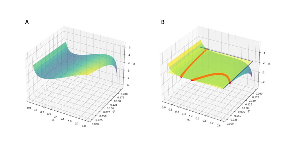
In a one-class system, there were only three densities corresponding to utility in the phase-separation region. However, in two-class systems, infinite combinations of () can exist for a specific utility value. These infinite density pairs are marked in red in Figure 7B. However, the interaction of the two classes of agents restricts the number of possible combinations of coexisting densities. The detailed analysis is provided in Appendix B.
VI Agent-based simulations: two-class system
Previously, we analyzed a one-class system and explained the qualitative changes in equilibrium configurations with changes in , , and the initial densities. Similar analysis can be performed for the two-class system.
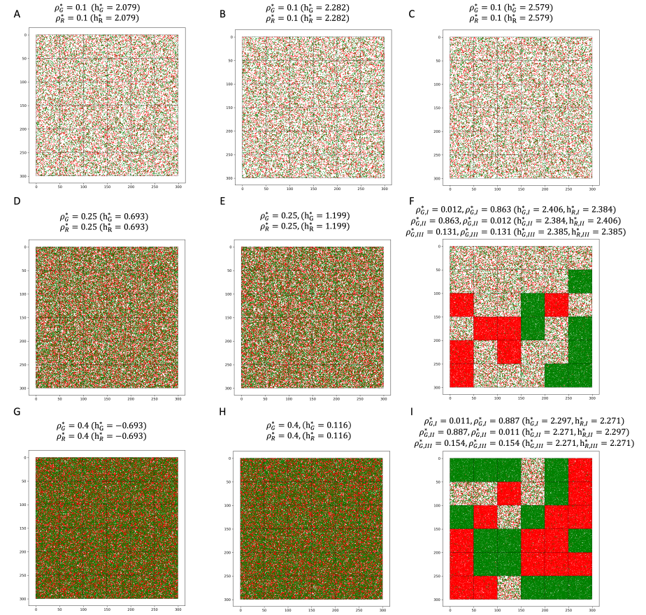
Consider Figure 8 showing equilibrium configurations of agents for different densities and s.
For simplicity, , and are assumed to be equal (= and and are assumed to be equal (=) in all the simulations reported in Figure 8. is fixed to 0 in all simulations. Each row of Figure 8 displays the equilibrium configurations for fixed densities of the two classes; in the upper row (A, B, C), in the middle row (D, E, F) and in the bottom row (G, H, I). Simulations were performed for three values of (). Each column in Figure 8 shows the equilibrium configuration for a fixed ; in the left column (A,D,G), in the middle column (B, E, H), and in the right column (C, F, I).
Like the one-class system, phase separation is not observed in the two-class system for small values of ( and ) (Figure 8A, B, D, E, G, H) for any densities. For , phase separation does not occur at .
However, separation is observed at higher densities ( and ). The nature of the game-theoretic potential can explain this behavior. Phase separation is observed when the potential-density surface is non-concave. In Appendix B, we explain the conditions for the concavity of the potential. For concave functions, the eigenvalues of the Hessian will be non-positive. When at least one eigenvalue is positive, the potential is non-concave. The Hessian eigenvalues are provided in Table 1 for each set of parameters reported in Figure 8. It can be seen from Table 1 that both Hessian eigenvalues (EV-1 and EV-2) are non-positive when and and therefore the potential is concave for configurations A, B, D, E, G and H in Figure 8.
Theoretically, it can be verified that the potential is concave in the entire density domain when . The potential is globally non-concave when and . For and , the potential is locally concave at the density (0.1,0.1) because, at this point, both eigenvalues of the Hessian are non-positive. Therefore, phase separation is not observed at this set of densities. However, one of the eigenvalues is positive at densities (0.25,0.25) and (0.4,0.4) (EV-1 for configuration F and EV-1 for configuration I). Therefore, the potential is non-concave, and as a consequence, phase separation is observed in configurations F and I.
| Configuration | EV-1 | EV-2 | Local | ||||
|---|---|---|---|---|---|---|---|
| in Figure 8 | concavity | ||||||
| A | 0 | 0 | 0.1 | 0.1 | -10 | -12.5 | Concave |
| B | 2.023 | 0 | 0.1 | 0.1 | -7.977 | -10.477 | Concave |
| C | 5 | 0 | 0.1 | 0.1 | -5. | -7.5 | Concave |
| D | 0 | 0 | 0.25 | 0.25 | -4 | -8 | Concave |
| E | 2.023 | 0 | 0.25 | 0.25 | -1.977 | -5.977 | Concave |
| F | 5 | 0 | 0.25 | 0.25 | 1 | -3 | Non-concave |
| G | 0 | 0 | 0.4 | 0.4 | -2.5 | -12.5 | Concave |
| H | 2.023 | 0 | 0.4 | 0.4 | -0.477 | -10.477 | Concave |
| I | 5 | 0 | 0.4 | 0.4 | 2.5 | -7.5 | Non-concave |
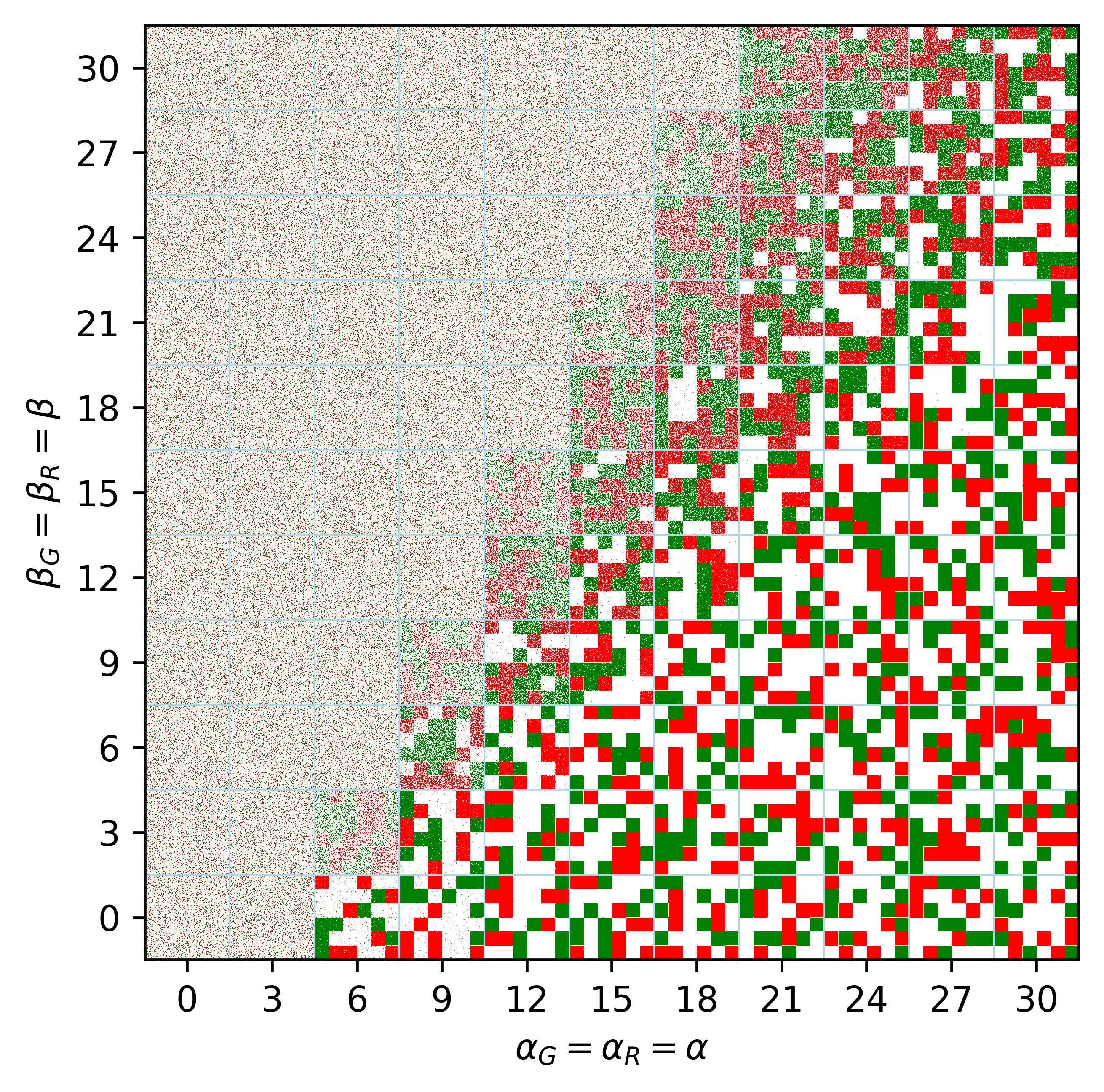
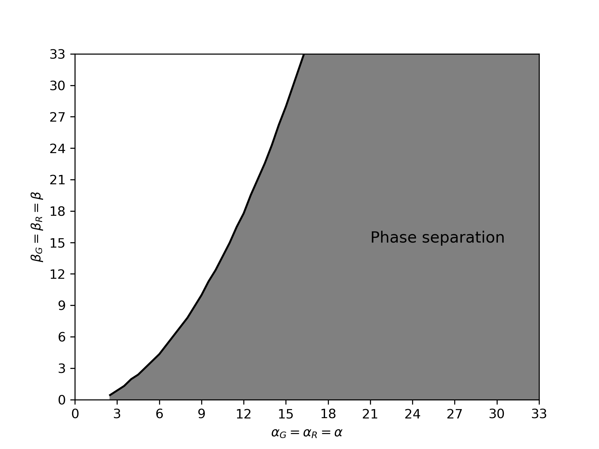
The parameter regime where phase separation occurs was theoretically predicted and plotted in Figure 13. Our numerical simulations agree with the theoretical predictions. The equilibrium agent configurations for a range of - values are shown in Figure 9. The and coordinates of each configuration indicate the values and used in the simulation. At low values of , there is no phase separation because there is not much incentive to get together. As increases, the agents come together. For any , the disutility due to crowding increases as increases. Mathematically, at low values of and high values of , the potential is concave (characterised by non-positive eigenvalues). For any fixed , larger values of results in non-concave potential. Similarly, for any fixed (), small values of leads to the non-concave potential. Therefore, phase separation is expected at large values of for a specific and at small values of for a specific . This behavior is observed in our simulations reported in Figure 9. All the simulations shown in Figure 9 performed for .
VII Methodology-Python Simulations
We developed Schelling-like models for one-class and two-class systems in the Python environment. The inputs to the program are the number of agents of each type, s and s. The number of agents in each class remains fixed through the simulation and is given by for the green agents and for the red agents. At each iteration, an agent and a vacant coordinate outside of the agent’s neighborhood are chosen at random. The agent’s utility in the current position is compared to the agent’s utility if the agent were to hypothetically move to the new vacant coordinate. If the agent’s utility is increased by moving to the new location, the agent moves and the respective density and utility values are updated. If not, the agent stays in its original position. Five million such offers are made to the agents. For the appropriate parameter set, the movement of the agents results in phase separation.
VIII Discussion
In this paper, we have presented a mathematical analysis of the decision dynamics of socioeconomic segregation in one- and two-class systems using a utility-driven game-theoretic model. For one-class systems, we showed both analytically and in simulations that the non-monotonic structure of the utility model causes social segregation. Depending on the parameters and , this usually occurs at higher densities. One can also predict and explain this segregation from the perspective of a system trying to maximize its game-theoretic potential. We have connected these two ideas by showing that the non-monotonic nature of the utility function results in non-concave potentials. The results of our agent-based simulations support these theoretical predictions. The parametric regime of segregation was identified using theory and confirmed by agent-based simulations.
More importantly, these predictions align with the results reported in the study by Nilforoshan et al.[1], where they observed social segregation in larger, denser cities. As noted, they observe that ”The consistent result that larger, denser cities are more segregated runs counter to the hypothesis that such cities promote socioeconomic mixing by attracting diverse individuals and constraining space in ways that oblige them to encounter one
other.” Our theory predicts this density-dependent segregation, as we discussed above.
They further state, ”Our results support the opposite hypothesis: big cities allow their inhabitants to seek out people who are more like themselves.” This is also expected in our theory, as seen in Fig. 6. As increases, the system tends to segregate. The parameter measures the social utility that an agent enjoys by being with others. In larger cities, as Nilforoshan et al.[1] study observes, there are many social options. This implies that will be higher in larger cities than in smaller ones. Therefore, as seen in Fig. 6, it is not surprising that the population segregates into different groups. In fact, this is expected by our model.
For the two-class system, as in the one-class system, social segregation occurs when the potential is non-concave. The negative-definiteness of the Hessian of the game-theoretic potential determines the concavity. Our simulations of two-class systems agree with the theoretical predictions. We have also determined the parametric regime of phase separation for the two-class systems.
Finally, we wish to direct the reader’s attention to an interesting observation. We note that the effective utility () enjoyed by the agents in the low- and high-density phases is the same (see Fig. 5F and I), as expected, because this is an arbitrage equilibrium. From a socioeconomic perspective, this is an interesting result. Interpreting the effective utility as a measure of ”happiness” or ”satisfaction”, we see that the two different socioeconomic groups are equally ”happy” in their respective environments. Even though they are segregated, they are both equally ”satisfied” with their lifestyles in our ideal society. To put this a bit more colorfully, the person enjoying a beverage with a small group of friends in a low-density small town is just as ”happy” as his/her larger city counterpart in a fancy and crowded restaurant in our ideal society. This harmonious outcome, despite segregation, is not necessarily bad. However, since ”happiness” is such an elusive concept, we wish to emphasize and caution that this ideal harmonious outcome, as envisioned in our model, might not occur in real-world societies. Although segregated populations enjoy the same effective utility in our ideal society, this might not be the case in the real world due to various social, economic, and political policies and constraints.
Appendix A Stability analysis of one-class systems
In Fig 2, we observe that for (blue curve) and (orange curve), (i.e. negative slope; recall that = ). In such a parameter regime, phase separation does not occur. However, for higher values of , regions with (i.e., positive slope) phase separation develop.
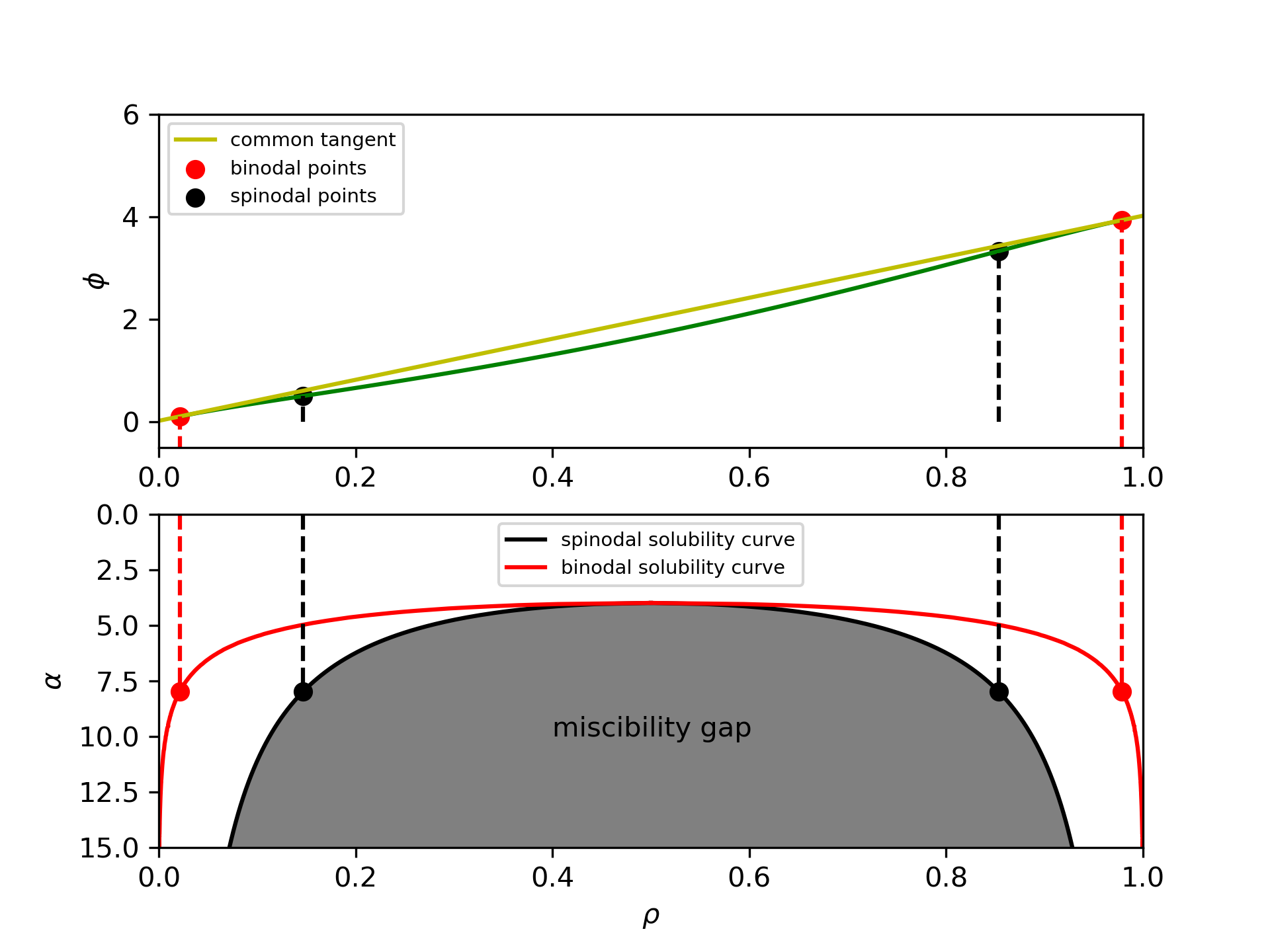
We better understand this from Fig. 10. The upper part of this figure shows the potential () vs the density () curve (in green) for , .
The plotted equation is
Spinodal points are shown as black dots, where = . The corresponding spinodal points are also shown in Fig. 2 as black dots on the green curve (, ). Fig. 10 also shows the binodal points (in red, connected by the common tangent line), where = . The corresponding binodal points are seen in Fig. 2 as red points connected by the red dotted line. As we see, the two binodal points enjoy the same utility (4.00), which is the arbitrage equilibrium.
The lower part of Fig. 10 shows the loci of binodal points (red curve) and spinodal points (black curve) for different values of (). As changes, the binodal and spinodal points change, and for () they disappear. Within the spinodal region, shown in dark gray, known as the miscibility gap in thermodynamics, a single phase of uniform density is unstable and would split into two phases of different densities. The reason is that the potential of a large group here is less than the sum of the two potentials of the low-density group and the high-density group at the binodal points.
We see this geometrically from the common tangent line connecting the binodal points, which is above the single-phase green curve between the spinodal points. Agents in such regions will be self-driven towards the high-density binodal point to increase their utility. Therefore, increases and the system splits into two groups of different densities.
Thus, for the green curve in Fig. 2, a self-organized, utility-driven, stable phase separation occurs spontaneously at the binodal points (red dotted line) at the arbitrage equilibrium. Although the miscibility gap is unstable, the region immediately outside it, between the black and red curves, is metastable. Beyond the red curve, one has a stable single phase of uniform density - no phase separation here.
In summary, for high values of (e.g., green curve in Fig. 2), combined with average densities in the miscibility gap, we observe the spontaneous emergence of two phases, high- and low-density groups of agents, at arbitrage equilibrium, socially driven by the self-actuated pursuit of maximum utility by the agents.
Intuitively, in the high-density phase, agents derive so much more benefit from the affinity term (due to the high ) that it more than compensates for the disutilities due to congestion and competition, thus yielding a high effective utility. Similarly, in the low-density phase, the benefits of reduced congestion and lower competition combined with increased option benefit more than compensate for the loss of utility from the affinity term.
Thus, every agent enjoys the same effective utility in one phase or the other at equilibrium. This causes equilibrium because, as noted, there is no more arbitrage incentive left for agents to switch neighborhoods.
As noted above, this analysis is mathematically equivalent to spinodal decomposition in statistical thermodynamics, with an important difference. In statistical thermodynamics, agents try to minimize their chemical potentials and the free energy of the system. Here, in statistical teleodynamics, agents try to maximize their utilities () and the game-theoretic potential (). In thermodynamics, chemical potentials are equal at phase equilibrium. In teleodynamics, the utilities are equal at the arbitrage equilibrium. The parallel is striking, but not surprising, because, as Venkatasubramanian has shown [8, 10], statistical teleodynamics is the generalization of statistical thermodynamics for goal-driven agents.
Appendix B Mathematical analysis of two-class systems
Consider the case, and . For now, assume that the equilibrium utility is (this is the equilibrium utility observed in the agent-based simulations). Due to the symmetry ( and ), both classes of agents are expected to exhibit identical behavior. This implies that if there exists a green-rich phase, referred to as Phase-I, with densities and , then there must also exist a red-rich phase, referred to as Phase-II with densities and such that and .
In addition to these phases, there may also exist other phases where both classes have the same densities. At equilibrium, the utilities of the two classes in each phase should be equal owing to the symmetry of the parameters, i.e.,
| (12) |
The constraint on the equilibrium densities emerging from Equation (12) is
| (13) |
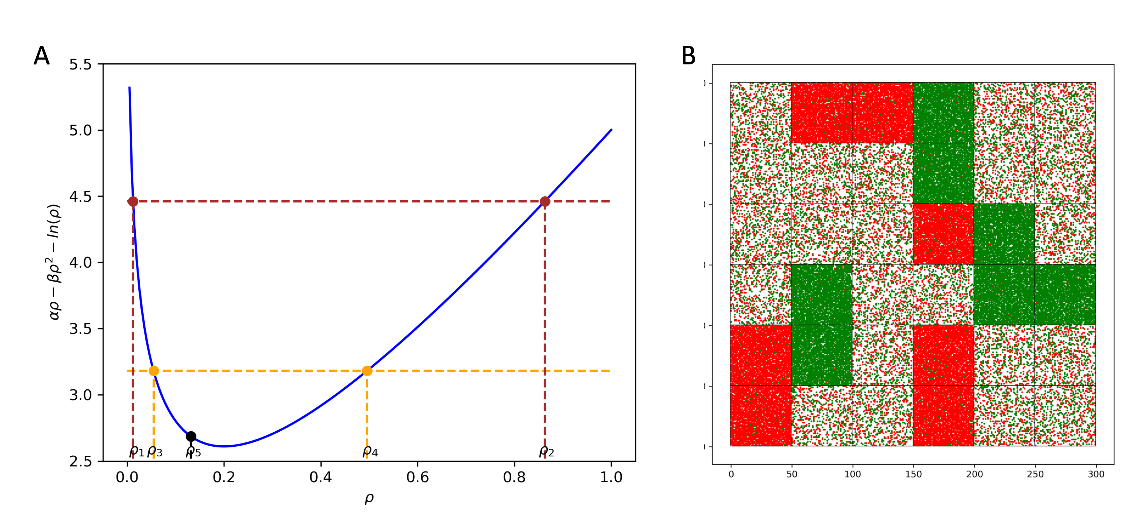
Let us determine the densities satisfying Eq.(12). Refer to the plot of shown in Figure 11 A. It can be observed that for a range of values of , there exist two densities () with the same value of . Two such solutions are shown with brown and orange points. The two densities represented by brown points have the same value of . Similarly, the two densities represented by the orange points have the same value of . Among the two brown points, let be the density of green agents, then will be the density of red agents in that phase (red-rich phase). Following the symmetry argument, there exists another phase (green-rich phase) with density for the red agents and density for the green agents. If any such pair of densities results in the equilibrium utility, , then that can be considered as a potential candidate for the densities in one of the phases.
Another possibility is the existence of other phases where both classes have equal density. An example of such a pair of densities is represented by the black point.
| Candidate Phase | h | ||||||
|---|---|---|---|---|---|---|---|
| I | 0.012 | 0.863 | 2.38 | -84.409 | -7.995 | -7.995 | -4.154 |
| II | 0.863 | 0.012 | 2.38 | -4.154 | -7.995 | -7.995 | -84.409 |
| III | 0132 | 0.132 | 2.38 | -3.951 | -1.358 | -1.358 | -3.951 |
| IV | 0.055 | 0.495 | 2.38 | -15.512 | -2.223 | -2.223 | 0.759 |
| V | 0.495 | 0.055 | 2.38 | 0.759 | -2.223 | -2.223 | -15.511 |
All densities marked in Figure 11A are solutions to Eq.(12), i.e., the density combinations (), (),(), () and () result in the same utility value, . Therefore, we have five potential phases into which the mixture may separate. Our extensive search in the density domain confirmed that there is no other solution to Eq. (12).
Can all these five phases coexist? Any phase with , , or is unstable. These derivatives evaluated in the five density pairs are provided in Table 2. Note that for Phases IV and V, one of the utility derivatives is positive. For Phase IV, , indicating that the red agents of other phases can move to Phase IV and increase their utility. These movements will increase the density of the red agents in Phase IV, and therefore Phase IV is unstable. Similar arguments can be applied to the green agents in Phase V. Therefore, for a phase to coexist with other phases, the utility derivatives must be non-positive. In summary, at equilibrium, we anticipate phases I, II, and III to coexist.
In addition to the above requirements, considering finite number of blocks and the definition of density of each class, the candidate density pairs must also satisfy the constraint that the number of blocks belonging to each phase must be an integer. Consider the separation of a mixture into three phases. Let the densities of the two classes in the three phases be represented as ,,,, and . The corresponding number of blocks in each phase is represented by , and . Then the conservation of the number of agents requires the following constraints to be satisfied.
| (14) | |||||
| (15) | |||||
| (16) |
where . These are soft constraints, meaning that minor differences in the calculated densities are expected in the simulations to ensure , and are integers.
The equilibrium configuration resulting from the simulation for and is provided in Figure 11B. As predicted by the theory, the simulation results in three phases. Moreover, the densities of the two classes in each phase observed in the simulation are exactly the same as those of the predictions.
Game-theoretic potential: Two-class system
The utilities of the two classes provided in Eq. (10) and (11) can be used to compute the game-theoretic potential of the system as shown in [13]. The potential is given by
| (17) | |||||
Parametric regime: Two-class system
For the one-class system, the parametric regime for phase separation was calculated from the derivative of the utility curve. For two-class systems, there are two independent densities, and therefore, one needs to consider the derivatives of utility with respect to both densities. In other words, one needs to analyze the Hessian of the potential to predict phase separation. Phase separation does not occur when the potential curve is purely concave. Phase separation can be expected for parameters that make the potential non-concave.
The Hessian of the potential is defined as:
| (18) |
Substituting the potential expression, we get,
| (19) |
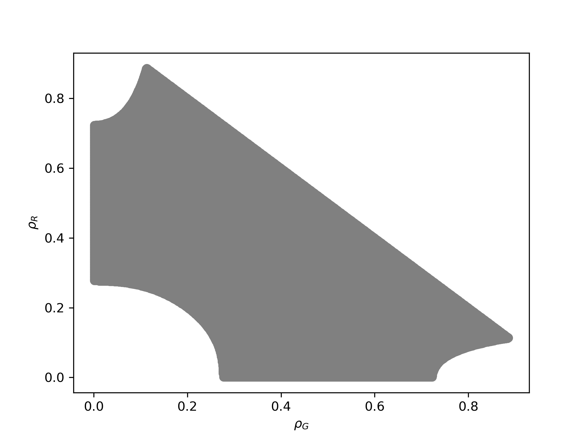
. Phase separation occurs when the density of the initial phase is in the shaded region.
.
The potential function is concave when the Hessian is negative semi-definite. The easiest way to check the negative semi-definiteness of the Hessian is to evaluate the sign of its eigenvalues. All the eigenvalues must be non-positive for a negative semi-definite matrix. Since we are interested in a non-concave potential function, our focus is on determining the parameter regime that leads to positive eigenvalues for the Hessian matrix.
Now, for any set of parameters , that result in a non-concave potential, there exists a region of densities where phase separation occurs. One of such density regions is shown for and in Figure 12. These densities were identified by evaluating the eigenvalues of the Hessian matrix. The points in the shaded region in Figure 12 represent densities of the two classes that result in at least one positive eigenvalue for the Hessian matrix.
Additionally, we performed a grid sweep in the parameter regime, searching for a non-concave potential function. The points in the shaded region in Figure 13 represent () values for which the potential function is non-concave in the density domain. The potential function is non-concave if the Hessian matrix has a positive eigenvalue for any pair of densities in the entire density domain.
References
- Nilforoshan et al. [2023] H. Nilforoshan, W. Looi, E. Pierson, B. Villanueva, N. Fishman, Y. Chen, J. Sholar, B. Redbird, D. Grusky, and J. Leskovec, Human mobility networks reveal increased segregation in large cities, Nature 624, 586 (2023).
- Schelling [1969] T. C. Schelling, Models of segregation, The American Economic Review 59, 488 (1969).
- Vinković and Kirman [2006] D. Vinković and A. Kirman, A physical analogue of the schelling model, Proceedings of the National Academy of Sciences 103, 19261 (2006).
- Gauvin et al. [2009] L. Gauvin, J. Vannimenus, and J.-P. Nadal, Phase diagram of a Schelling segregation model, The European Physical Journal B - Condensed Matter and Complex Systems 70, 293 (2009).
- Dall’Asta et al. [2008] L. Dall’Asta, C. Castellano, and M. Marsili, Statistical physics of the schelling model of segregation, Journal of Statistical Mechanics: Theory and Experiment 2008, L07002 (2008).
- Avetisov et al. [2018] V. Avetisov, A. Gorsky, S. Maslov, S. Nechaev, and O. Valba, Phase transitions in social networks inspired by the schelling model, Physical Review E 98, 032308 (2018).
- Grauwin et al. [2009] S. Grauwin, E. Bertin, R. Lemoy, and P. Jensen, Competition between collective and individual dynamics, Proceedings of the National Academy of Sciences 106, 20622 (2009), https://www.pnas.org/content/106/49/20622.full.pdf .
- Venkatasubramanian [2017] V. Venkatasubramanian, How Much Inequality Is Fair?: Mathematical Principles of a Moral, Optimal, and Stable Capitalist Society (Columbia University Press, 2017).
- Venkatasubramanian et al. [2015] V. Venkatasubramanian, Y. Luo, and J. Sethuraman, How much inequality in income is fair?: A microeconomic game theoretic perspective, Physica A: Statistical Mechanics and its Applications 435, 120 (2015).
- Venkatasubramanian et al. [2022] V. Venkatasubramanian, A. Sivaram, and L. Das, A unified theory of emergent equilibrium phenomena in active and passive matter, Computers & Chemical Engineering 164, 107887 (2022).
- Kanbur and Venkatasubramanian [2020] R. Kanbur and V. Venkatasubramanian, Occupational arbitrage equilibrium as an entropy maximizing solution, The European Physical Journal Special Topics 229, 1661 (2020).
- Sivaram and Venkatasubramanian [2022] A. Sivaram and V. Venkatasubramanian, Arbitrage equilibrium, invariance, and the emergence of spontaneous order in the dynamics of birds flocking, ArXiv:2207.13743v4 (2022).
- Sandholm [2010] W. H. Sandholm, Population games and evolutionary dynamics (MIT press, 2010).
- Cahn [1961] J. W. Cahn, On spinodal decomposition, Acta metallurgica 9, 795 (1961).
- Favvas and Mitropoulos [2008] E. Favvas and A. C. Mitropoulos, What is spinodal decomposition, Journal of Engineering Science and Technology Review 1, 25 (2008).