Energy-Energy Correlation in the back-to-back
region at N³LL+NNLO in QCD

Ugo Giuseppe Aglietti^(a) and  Giancarlo Ferrera^(b)

^(a) Dipartimento di Fisica, Università di Roma “La Sapienza” and

INFN, Sezione di Roma I-00185 Rome, Italy

^(b) Dipartimento di Fisica, Università di Milano and

INFN, Sezione di Milano, I-20133 Milan, Italy

Abstract

We consider the Energy-Energy Correlation function in electron-positron annihilation to hadrons. We concentrate on the back-to-back region, performing all-order resummation of the logarithmically enhanced contributions in QCD perturbation theory, up to next-to-next-to-next-to-leading logarithmic (N³LL) accuracy. Away from the back-to-back region, we consistently combine resummed predictions with the known fixed-order results up to next-to-next-to-leading order (NNLO). All perturbative terms up to order $\alpha_{S}^{3}$ are included in our calculation, which exactly reproduces, after integration over the angular separation variable, the next-to-next-to-next-to-leading order (N³LO) result for the total cross section. We regularize the Landau singularity of the QCD coupling within the so-called Minimal Prescription. We exhibit and discuss the reduction of the perturbative scale dependence of distributions at higher orders, as a means to estimate the corresponding residual perturbative uncertainty. We finally present an illustrative comparison with LEP data.

This paper is dedicated to the memory of Stefano Catani,
wonderful person, outstanding scientist.

March 2024

1 Introduction

One of the classical methods to test QCD predictions and obtain a precise determination of the strong coupling $\alpha_{S}$ at a reference scale, concerns the analysis of (infrared-safe) shape variable distributions in high-energy electron-positron annihilation to hadrons. In the two-jet region, in which the high-energy hadrons in final states are collimated into two opposite directions, the ordinary QCD perturbative expansion does not provide a good approximation, because its coefficients contain large double logarithms of infrared (soft and collinear) origin, the so-called Sudakov logarithms. The resummation to all orders in $\alpha_{S}$ of such logarithms for shape variables has been formulated in the classic paper [1].

Among the various shape variables, the Energy-Energy Correlation (EEC) function [2] has received considerable interest over the years both from the experimental and theoretical side. This function describes the distribution of the angular separation (usually called ”$\chi$”) of the hard particle pairs in the events (the precise definition will be given below in Eq. (1)). The resummation of Sudakov logarithms in the back-to-back region ($\chi\to\pi^{-}$) for the EEC function has been achieved in full QCD at next-to-leading logarithmic (NLL) [3, 4, 5, 6, 7], and at next-to-next-to-leading logarithmic (NNLL) [8, 9, 10] accuracies. More recently, the EEC function has also been analyzed within the framework of the Soft-Collinear Effective Theory (SCET) up to next-to-next-to-next-to-leading logarithmic (N³LL) accuracy [11, 12] and beyond [13]. The perturbative expansion of the EEC function also contains large (single) logarithmic corrections in the forward region ($\chi\to 0^{+}$), where two or more energetic hadrons are produced at small angular separations. However, these effects are physically quite different, being of hard-collinear nature [14]; in this paper we will focus on the back-to-back region.

Away from the endpoints of the angular domain, the perturbative series is well behaved, so that calculations based on the truncation at a fixed order in $\alpha_{S}$ are theoretically justified. Since hadron production away from the back-to-back region has to be accompanied by the radiation of at least one hard recoiling parton, the leading-order (LO) term for this observable is $\mathcal{O}(\alpha_{S})$. The LO distribution of the EEC function has been originally calculated in the late seventies in Ref. [2]. The next-to-leading-order (NLO) QCD corrections have been known numerically long ago [15, 16] and have been recently computed analytically in Ref. [17]. The next-to-next-to-leading-order (NNLO) correction has been obtained by numerical Monte Carlo integration of the fully differential cross section for three-jet production in electron-positron annihilation at NNLO order in QCD [18, 19]. The behavior of the EEC function in the back-to-back region has been determined analytically at next-to-next-to-next-to-leading order (N³LO) in [12].

In general, resummed and fixed-order calculations have to be consistently combined with each other at intermediate values of the angular separation, where they are both valid, in order to obtain accurate QCD predictions on a wide kinematical region.

In this work, we perform the resummation of infrared Sudakov logarithms in the back-to-back region of the EEC function up to N³LL accuracy in QCD, matching with the corresponding fixed-order results of Refs. [2, 17, 9] up to NNLO. All perturbative terms up to N³LO, i.e. up to $\mathcal{O}(\alpha_{S}^{3})$, are consistently included ; in particular, we determine the N³LO coefficients of the hard-virtual factor $H(\alpha_{S})$ and of the of single logarithmic function $B(\alpha_{S})$ of the Sudakov form factor from the calculation in Ref. [12]. Thanks to the unitarity constraint of the resummation formalism [20], our calculation exactly reproduce, after integration over the angular separation variable $\chi$, the corresponding fixed-order result for the total cross section of electron-positron annihilation into hadrons up to N³LO [25, 26].

The paper is organized as follows. In Sec. 2 we define the EEC observable and consider its standard, i.e. fixed-order perturbative expansion. In Sec. 3 we discuss the QCD impact-parameter ($b$-)space resummation formalism for the EEC distribution, which has a structure similar to (and simpler than) the one for the transverse-momentum ($q_{T}$-)distribution in hadron-hadron collisions  [21, 22, 23, 20]. In Sec. 4 we provide explicit formulae for the coefficients which are needed for the resummation up to N³LL+NNLO accuracy (including the hard-virtual coefficients up to N³LO). In Sec. 5 we present explicit formulae for the remainder component of the EEC function, which is relevant outside the back-to-back region, again at NNLO. In Sec. 6 we exhibit and discuss the dependence of our predictions on auxiliary perturbative scales at NLL+LO, NNLL+NLO and N³LL+NNLO. Such scale dependence is used to estimate the corresponding perturbative uncertainty of our prediction. We also present an illustrative comparison with experimental data from the OPAL Collaboration at LEP accelerator [24]. While we anticipate that the N³LL+NNLO prediction provides the best perturbative description of experimental data, we also remark that there is still a sizable difference between data and theory, especially in the peak region, where most data are taken, which calls for an explicit inclusion of Non-Perturbative (NP) QCD effects. A more detailed phenomenological analysis, together with the introduction of a consistent NP model, is left for a future work. Finally, Sec. 7 contains the conclusions of our analysis.

2 Energy-Energy Correlation Function

The differential distribution for the Energy-Energy Correlation (EEC) function in electron-positron annihilation to hadrons is defined as

$$\frac{d\Sigma}{d\cos\chi}\,=\,\sum_{i,j=1}^{n}\int\frac{E_{i}}{Q}\,\frac{E_{j}}{Q}\,\delta\left(\cos\chi\,-\,\cos\theta_{ij}\right)\,d\sigma\,,$$ (1)

where $Q\equiv\sqrt{s}$ is the center-of-mass energy of the colliding leptons, $n\geq 2$ is the number of hadrons in the (physical) event (partons in the perturbative QCD calculation) and $\theta_{ij}$ is the angle between the spatial momenta $\vec{p}_{i}$ and $\vec{p}_{j}$ of hadrons $i$ and $j$ respectively ($0\leq\theta_{ij}\leq\pi$). Note that self-correlation terms, namely the terms for $i=j$ (for which $\theta_{ij}\equiv 0$), are included in the (double) sum. This distribution characterizes the angular separation of pairs of hard hadrons in the events. By integrating over all the relative angles, the kinematical constraint given by the $\delta$-function disappears and the total cross section ($\sigma_{\rm tot}$) is recovered:

$$\int\limits_{-1}^{+1}\frac{d\Sigma}{d\cos\chi}\,d\cos\chi\,=\,\int\left(\sum_{i=1}^{n}\frac{E_{i}}{Q}\right)^{2}\,d\sigma\,=\,\sigma_{\rm tot}\,,$$ (2)

where we have used the relation

$$\sum_{i=1}^{n}\frac{E_{i}}{Q}\,=\,1\,.$$ (3)

In the center-of-mass frame (where $\vec{P}_{tot}=\sum_{i=1}^{n}\vec{p}_{i}=0$), at lowest order in the expansion in the QCD coupling $\alpha_{S}$, the final state consists of a back-to-back quark-antiquark pair ($E_{1}=E_{2}=Q/2$), implying:

$$\frac{1}{\sigma_{0}}\,\frac{d\Sigma}{d\cos\chi}\,=\,\frac{1}{2}\,\delta(1-\cos\chi)\,+\,\frac{1}{2}\,\delta(1+\cos\chi)\,+\,\mathcal{O}\left(\alpha_{S}\right)\,,$$ (4)

where $\sigma_{0}$ is the total cross section in Born approximation for the process $e^{+}e^{-}\mapsto\mathrm{hadrons}$. Let us remark that the factor 2 comes from the fact that the pair $(1,2)$ is counted two times in the double sum above over $i$ and $j$. The lowest-order distribution then consists of two peaks of the same strength, at the physical endpoints, $\chi=0$ and $\chi=\pi$ .

We will mostly consider the back-to-back region,

$$\chi\,\lesssim\,\pi\quad\mathrm{or,\,\,equivalently,}\,\,\pi\,-\,\chi\,\ll\,1.$$ (5)

To discuss (perturbative) higher-order corrections, it is convenient to introduce the unitary variable $z$ defined as:

$$z\,\equiv\,\frac{1\,-\,\cos\chi}{2}\,=\,\sin^{2}\left(\frac{\chi}{2}\right)\,,\qquad(0\leq z\leq 1)\,.$$ (6)

In the back-to-back region, it is also useful to consider the quantity

$$1\,-\,z\,=\,\frac{1\,+\,\cos\chi}{2}\,=\,\cos^{2}\left(\frac{\chi}{2}\right)\,\simeq\,\left(\frac{\pi\,-\,\chi}{2}\right)^{2}\qquad\mathrm{for}\,\,\,\pi\,-\,\chi\,\ll\,1.$$ (7)

In terms of the kinematical variable $z$, the lowest-order EEC function simply reads:

$$\frac{1}{\sigma_{0}}\,\frac{d\Sigma}{dz}\,=\,\frac{1}{2}\,\delta(1\,-\,z)\,+\,\frac{1}{2}\,\delta(z)\,+\,\mathcal{O}\left(\alpha_{S}\right)\,.$$ (8)

The general perturbative QCD expansion of the EEC function, normalized to the radiatively-corrected total cross section is written as:

$$\frac{1}{\sigma_{\rm tot}}\,\frac{d\Sigma}{dz} = \frac{1}{2}\big{[}\delta(1\,-\,z)\,+\,\delta(z)\big{]}\,+\,\mathcal{A}(z)\,\frac{\alpha_{S}}{\pi}\,+\,\mathcal{B}(z)\left(\frac{\alpha_{S}}{\pi}\right)^{2}$$

$$+ \,\mathcal{C}(z)\left(\frac{\alpha_{S}}{\pi}\right)^{3}\,+\,\mathcal{O}\left(\alpha_{S}^{4}\right).$$

The first-order function $\mathcal{A}(z)$ has been evaluated in the late seventies in [2]; by including the endpoints contributions [14] it reads:

$$\mathcal{A}(z) = \frac{4}{3}\Bigg{\{}-\frac{1}{2}\left[\frac{\log(1-z)}{1-z}\right]_{+}-\frac{3}{4}\left[\frac{1}{1-z}\right]_{+}+\frac{3}{8}\left[\frac{1}{z}\right]_{+}$$

$$- \left(\frac{z_{2}}{2}+\frac{11}{8}\right)\delta(1-z)-\frac{23}{96}\delta(z)$$

$$+ \frac{1}{8z^{5}}\left[4\left(-z^{4}-z^{3}+3z^{2}-15z+9\right)\log(1-z)-9z^{4}-6z^{3}-42z^{2}+36z\right]\Bigg{\}}.$$

The second-order function $\mathcal{B}(z)$ has been calculated analytically in Ref. [17], after the numerical computation in Ref. [15, 16]. Finally, the third-order function $\mathcal{C}(z)$ has been evaluated only numerically in the whole $z$ range in Refs. [18, 19]; its large $z$ behavior has been evaluated analytically in Ref. [12].

As can be seen from Eq.(2) and from a higher-order analysis, in the back-to-back region, large logarithms of infrared origin of the form

$$\alpha_{S}^{n}\left[\frac{\ln^{k}(1-z)}{1-z}\right]_{+},\qquad n=1,2,3,\cdots,\quad 0\leq k\leq 2n-1,$$ (11)

do occur in the perturbative expansion. The subscript ’+’ denotes the customary plus regularization of distributions:

$$\int\limits_{0}^{1}\left[F(z)\right]_{+}\varphi(z)\,dz\,\equiv\,\int\limits_{0}^{1}F(z)\big{[}\varphi(z)\,-\,\varphi(1)\big{]}\,dz,$$ (12)

with $\varphi(z)$ an arbitrary test (i.e. smooth) function. The occurrence of such large logarithmic terms in the back-to-back region ($z\to 1^{-}$) spoils the convergence of the ordinary, fixed order perturbative expansion. To have a reliable QCD prediction, these logarithms have to be resummed to all orders of $\alpha_{S}$; for consistency reasons, as we are going to show, one has also to include all the contribution proportional to $\delta(1-z)$.

3 Resummation of Energy-Energy Correlation in the back-to-back region

The differential distribution for the EEC function in Eq. (2) is decomposed as:

$$\frac{1}{\sigma_{\rm tot}}\,\frac{d\Sigma}{dz}\,=\,\frac{1}{\sigma_{\rm tot}}\,\frac{d\Sigma_{(\rm res.)}}{dz}\,+\,\frac{1}{\sigma_{\rm tot}}\,\frac{d\Sigma_{(\rm fin.)}}{dz}\,.$$ (13)

The first term on the right-hand side of Eq.(13) is the resummed $(\rm res.)$ component, containing all the logarithmically-enhanced contributions at large $z$ (see Eq.(11)), to be resummed to all orders (i.e. for any $n=1,2,3,\cdots$) together with the $\delta(1-z)$ contributions, while the second term, the finite $(\rm fin.)$ component, free from such contributions, can be computed by standard, fixed-order perturbation theory.

3.1 Resummed term

In order to consistently take into account the kinematics constraint of transverse-momentum conservation in multiple parton emissions, the resummation program has to be carried out in the impact-parameter space or $b$-space ($b$ is the conjugated variable to $Q\sqrt{1-z}$) [21] where the back-to-back region $1-z\ll 1$ corresponds to the region $bQ\gg 1$. The EEC distribution in the physical $z$-space is then recovered by performing an inverse Fourier-Bessel transformation with respect to the impact parameter $b$ [3, 4, 5, 6, 7]:

$$\frac{1}{\sigma_{\rm tot}}\,\frac{d\Sigma_{\rm(res.)}}{dz}\,=\,\frac{1}{2}\,H\left(\alpha_{S}\right)\int\limits_{0}^{\infty}d(Qb)\,\frac{Qb}{2}\,J_{0}\left(\sqrt{1-z}\,Qb\right)\,S\left(Q,b\right)\,,$$ (14)

where $J_{0}(x)$ is the Bessel function of first kind $J_{\nu}(x)$ with zero index, $\nu=0$. According to Eq.(14) the resummed component of the EEC distribution has been factorized, in $b$-space, in two factors, namely $H(\alpha_{S})$ and $S(Q,b)$. The function $H\left(\alpha_{S}\right)$ in Eq.(14) is a $b$-independent, hard factor, including hard-virtual contributions at a scale $q\sim Q$; it contains all the terms that behave as constants in the limit $b\to\infty$ which correspond, in a minimal factorization scheme, to corrections proportional to $\delta(1-z)$ in the physical (angle) space. The function $S\left(Q,b\right)$ in Eq.(14) is the QCD Sudakov form factor, which resums to all orders, in $b$-space, the large logarithmic corrections of the type $\alpha_{S}^{n}\ln^{k}(Q^{2}b^{2})$ ($n=1,2,3\dots$, $1\leq k\leq 2n$). The latter are divergent when $b\to+\infty$ and correspond, in physical space, to the infrared logarithms in Eq.(11). Note that the (perturbative) factorization of constants and logarithmic terms in Eq.(14) involves some degree of arbitrariness, since the argument of the large logarithms can always be rescaled as:

$$\ln\left(\frac{Q^{2}\,b^{2}}{b_{0}^{2}}\right)\,=\,\ln\left(\frac{\mu_{Q}^{2}\,b^{2}}{b_{0}^{2}}\right)\,+\,\ln\left(\frac{Q^{2}}{\mu_{Q}^{2}}\right),$$ (15)

where we have introduced the coefficient $b_{0}\equiv 2\exp\left(-\gamma_{E}\right)\simeq 1.123$ ($\gamma_{E}=0.5772\cdots$ is the Euler-Mascheroni constant) . The rescaling in Eq. (15) is governed by the arbitrary (but independent on $b$) energy scale $\mu_{Q}$, called resummation scale [20]. This scale has to be considered of the order of the hard scale, $\mu_{Q}\sim Q$, so that $\ln(Q^{2}/\mu_{Q}^{2})$ is a constant term $\mathcal{O}(1)$; in other words, it is assumed not to be a large logarithm. That implies, in particular, that the $\mu_{Q}$-dependent terms have not to be exponentiated in $S(Q,b)$, but rather factorized in $H(\alpha_{S})$ which therefore explicitly depends on $\mu_{Q}$. The large (logarithmic) expansion parameter is thus:

$$L\,\equiv\,\ln\left(\frac{\mu_{Q}^{2}\,b^{2}}{b_{0}^{2}}\right)\,$$ (16)

with $L\gg 1$ for $b\gg b_{0}/\mu_{Q}\sim 1/Q$. Let us notice that the role played by the resummation scale $\mu_{Q}$ in the resummation formalism is analog to the role played by the renormalization scale $\mu_{R}$ in the context of renormalization. If evaluated exactly, i.e. by including all the perturbative orders, the resummed cross section, Eq. (14), does not depend on $\mu_{Q}$. On the contrary, when evaluated approximately, i.e. at some level of logarithmic accuracy, the resummed cross section exhibits a residual dependence on $\mu_{Q}$. We choose the central or reference value of the resummation scale to be equal to the hard scale, $\mu_{Q}=Q$. Actually, conventional variations of $\mu_{Q}$ around its central value can be used to estimate the uncertainty coming from yet uncalculated higher-order logarithmic terms.

The resummation of the logarithmic contributions is achieved by showing that the Sudakov form factor can be expressed in the following exponential form [3, 6, 20]:

$$S\left(Q,b\right)\,=\,\exp\Bigg{\{}-\int\limits_{b_{0}^{2}/b^{2}}^{\mu_{Q}^{2}}\frac{dq^{2}}{q^{2}}\left[A\left(\alpha_{S}(q^{2})\right)\ln\left(\frac{Q^{2}}{q^{2}}\right)\,+\,B\left(\alpha_{S}(q^{2})\right)\right]\Bigg{\}}.$$ (17)

The double-logarithmic function $A(\alpha_{S})$ describes the effects of both soft and collinear parton emission off the primary partons in the process (a light quark-antiquark pair in our case), while the single-logarithmic function $B(\alpha_{S})$ describes the effect of soft wide-angle radiation or hard collinear radiation at scales $1/b\lesssim q\lesssim Q$ (since the EEC function is an infrared-safe observable, soft-virtual cancellation suppresses both soft and collinear contributions at energy/momentum scales $q\lesssim 1/b$). The functions $A(\alpha_{S})$, $B(\alpha_{S})$ and $H\left(\alpha_{S}\right)$ possess ordinary (i.e. without logarithmic coefficients) perturbative expansions in powers of $\alpha_{S}$ of the form:

$$A(\alpha_{S}) = \sum_{n=1}^{\infty}A_{n}\,\left(\frac{\alpha_{S}}{\pi}\right)^{n}\,,$$ (18)

$$B(\alpha_{S}) = \sum_{n=1}^{\infty}B_{n}\,\left(\frac{\alpha_{S}}{\pi}\right)^{n}\,,$$ (19)

$$H(\alpha_{S}) = 1\,+\,\sum_{n=1}^{\infty}H_{n}\,\left(\frac{\alpha_{S}}{\pi}\right)^{n}\,.$$ (20)

The integral on the right hand side (r.h.s.) of Eq. (17) can be explicitly evaluated order-by-order in $\alpha_{S}$ by using the iterative solution of the renormalization group equation for the QCD coupling:

$$\frac{d\ln\alpha_{S}(\mu_{R}^{2})}{d\ln\mu_{R}^{2}}\,=\,\beta(\alpha_{S})\,=\,-\,\beta_{0}\,\frac{\alpha_{S}}{\pi}\,-\,\beta_{1}\left(\frac{\alpha_{S}}{\pi}\right)^{2}\,-\,\beta_{2}\left(\frac{\alpha_{S}}{\pi}\right)^{3}\,-\,\beta_{3}\left(\frac{\alpha_{S}}{\pi}\right)^{4}\,-\,\cdots\,,$$ (21)

where $\mu_{R}$ is the renormalization scale.

The solution of Eq.(21) up to N³LO is given by:

$$\alpha_{S}(q^{2}) = \frac{\alpha_{S}}{l}\left\{1\,-\,\frac{\alpha_{S}}{\pi l}\frac{\beta_{1}}{\beta_{0}}\ln l+\left(\frac{\alpha_{S}}{\pi l}\right)^{2}\left[\frac{\beta_{1}^{2}}{\beta_{0}^{2}}(\ln^{2}l-\ln l+l-1)-\frac{\beta_{2}}{\beta_{0}}(l-1)\right]\right.$$ (22)

$$+ \left(\frac{\alpha_{S}}{\pi l}\right)^{3}\left[\frac{\beta_{1}^{3}}{\beta_{0}^{3}}\left(-\ln^{3}l+\frac{5}{2}\ln^{2}l-2(l-1)\ln l-\frac{(l-1)^{2}}{2}\right)\right.$$

$$~{}~{}~{}~{}~{}~{}~{}~{}~{}+\left.\left.\frac{\beta_{1}\beta_{2}}{\beta_{0}^{2}}\big{(}(l-1)l+(2l-3)\ln l\big{)}+\frac{\beta_{3}}{\beta_{0}}\frac{(1-l^{2})}{2}\right]+\mathcal{O}(\alpha_{S}^{4})\right\},$$

with $\alpha_{S}\equiv\alpha_{S}(\mu_{R}^{2})$ and $l\equiv 1+\beta_{0}\alpha_{S}/\pi\ln(q^{2}/\mu_{R}^{2})$.

After the analytic integration in the exponent in Eq. (17), the Sudakov form factor can be recast in the following form [23, 8]:

$$S(Q,b)\,=\,\exp\left\{L\,g_{1}(\lambda)\,+\,g_{2}(\lambda)\,+\,\frac{\alpha_{S}}{\pi}g_{3}(\lambda)\,+\,\left(\frac{\alpha_{S}}{\pi}\right)^{2}g_{4}(\lambda)\,+\,\sum_{n=5}^{+\infty}\left(\frac{\alpha_{S}}{\pi}\right)^{n-2}g_{n}(\lambda)\right\}\,,$$ (23)

where the variable

$$\lambda\,\equiv\,\frac{\alpha_{S}}{\pi}\,\beta_{0}\,L\,,$$ (24)

is assumed to be $\mathcal{O}(1)$. The exponent on the r.h.s. of Eq. (23) has thus a customary perturbative expansion in powers of $\alpha_{S}$, with $\lambda$-dependent coefficients. The truncation of such (function) series at a given order resums an infinite series of logarithmic corrections. The leading-logarithmic (LL) approximation is provided by the function $g_{1}(\lambda)$, the NLL approximation requires also the inclusion of the function $g_{2}(\lambda)$, the NNLL and N³LL approximations require also the functions $g_{3}(\lambda)$ and $g_{4}(\lambda)$ respectively, and so on. The resummation functions $g_{n}(\lambda)$, with $1\leq n\leq 4$, have the following explicit expressions:

$$g_{1}(\lambda)=\frac{A_{1}}{\beta_{0}}\,\frac{\lambda+\ln(1-\lambda)}{\lambda}\,,$$ (25)

$$g_{2}(\lambda) = -\frac{A_{2}}{\beta_{0}^{2}}\left[\frac{\lambda}{1-\lambda}+\ln(1-\lambda)\right]+\frac{{B}_{1}}{\beta_{0}}\ln(1-\lambda)$$ (26)

$$+ \frac{A_{1}\beta_{1}}{\beta_{0}^{3}}\left[\frac{\lambda}{1-\lambda}+\frac{1}{2}\ln^{2}(1-\lambda)+\frac{\ln(1-\lambda)}{1-\lambda}\right]$$

$$+ \frac{A_{1}}{\beta_{0}}\left[\frac{\lambda}{1-\lambda}+\ln(1-\lambda)\right]\ln\left(\frac{\mu_{Q}^{2}}{\mu_{R}^{2}}\right)\,,$$

$$g_{3}(\lambda) = -\frac{A_{3}}{2\beta_{0}^{2}}\frac{\lambda^{2}}{(1-\lambda)^{2}}-\frac{{B}_{2}}{\beta_{0}}\frac{\lambda}{1-\lambda}-\frac{A_{2}\beta_{1}}{2\beta_{0}^{3}}\frac{\lambda(2-3\lambda)+2(1-2\lambda)\ln(1-\lambda)}{(1-\lambda)^{2}}$$ (27)

$$+ \frac{A_{1}\beta_{2}}{2\beta_{0}^{3}}\left[\lambda\frac{2-3\lambda}{(1-\lambda)^{2}}+2\ln(1-\lambda)\right]+\frac{{B}_{1}\beta_{1}}{\beta_{0}^{2}}\frac{\lambda+\ln(1-\lambda)}{1-\lambda}$$

$$+ \frac{A_{1}\beta_{1}^{2}}{2\beta_{0}^{4}}\frac{\lambda^{2}+(1-2\lambda)\ln^{2}(1-\lambda)+2\lambda(1-\lambda)\ln(1-\lambda)}{(1-\lambda)^{2}}$$

$$- \frac{A_{1}}{2}\frac{\lambda^{2}}{(1-\lambda)^{2}}\ln^{2}\left(\frac{\mu_{Q}^{2}}{\mu_{R}^{2}}\right)+\Bigg{[}\frac{A_{2}}{\beta_{0}}\frac{\lambda^{2}}{(1-\lambda)^{2}}+{B}_{1}\frac{\lambda}{1-\lambda}$$

$$+ \frac{A_{1}\beta_{1}}{\beta_{0}^{2}}\frac{(1-2\lambda)\ln(1-\lambda)+\lambda(1-\lambda)}{(1-\lambda)^{2}}\Bigg{]}\ln\left(\frac{\mu_{Q}^{2}}{\mu_{R}^{2}}\right)\,,$$

$$g_{4}(\lambda) = -\frac{A_{4}}{6\beta_{0}^{2}}\lambda^{2}\frac{3-\lambda}{(1-\lambda)^{3}}-\frac{{B}_{3}}{2\beta_{0}}\lambda\frac{2-\lambda}{(1-\lambda)^{2}}+\frac{{B}_{2}\beta_{1}}{2\beta_{0}^{2}}\frac{2\ln(1-\lambda)+\lambda(2-\lambda)}{(1-\lambda)^{2}}$$ (28)

$$- \frac{A_{3}\beta_{1}}{12\beta_{0}^{3}}\frac{\lambda\left(5\lambda^{2}-15\lambda+6\right)+6(1-3\lambda)\ln(1-\lambda)}{(1-\lambda)^{3}}-\frac{2A_{2}\beta_{2}}{3\beta_{0}^{3}}\frac{\lambda^{3}}{(1-\lambda)^{3}}$$

$$+ \frac{A_{2}\beta_{1}^{2}}{12\beta_{0}^{4}}\frac{\lambda\left(11\lambda^{2}-9\lambda+6\right)+6(1-3\lambda)\ln^{2}(1-\lambda)+6(1-\lambda)\ln(1-\lambda)}{(1-\lambda)^{3}}$$

$$+ \frac{A_{1}\beta_{3}}{12\beta_{0}^{3}}\left[\lambda\frac{7\lambda^{2}-15\lambda+6}{(1-\lambda)^{3}}+6\ln(1-\lambda)\right]$$

$$- \frac{A_{1}\beta_{1}^{3}}{6\beta_{0}^{5}}\frac{\lambda^{3}+3\lambda^{2}(1+\lambda)\ln(1-\lambda)+3\lambda\ln^{2}(1-\lambda)+(1-3\lambda)\ln^{3}(1-\lambda)}{(1-\lambda)^{3}}$$

$$- \frac{A_{1}\beta_{1}\beta_{2}}{12\beta_{0}^{4}}\frac{\lambda\left(5\lambda^{2}-15\lambda+6\right)-6\left(2\lambda^{3}-2\lambda^{2}+3\lambda-1\right)\ln(1-\lambda)}{(1-\lambda)^{3}}$$

$$- \frac{{B}_{1}\beta_{2}}{2\beta_{0}^{2}}\frac{\lambda^{2}}{(1-\lambda)^{2}}+\frac{{B}_{1}\beta_{1}^{2}}{2\beta_{0}^{3}}\frac{\lambda^{2}-\ln^{2}(1-\lambda)}{(1-\lambda)^{2}}+\frac{A_{1}\beta_{0}}{6}\lambda^{2}\frac{3-\lambda}{(1-\lambda)^{3}}\ln^{3}\left(\frac{\mu_{Q}^{2}}{\mu_{R}^{2}}\right)$$

$$- \Bigg{[}\frac{A_{2}}{2}\lambda^{2}\frac{3-\lambda}{(1-\lambda)^{3}}+\frac{A_{1}\beta_{1}}{2\beta_{0}}\frac{\lambda+(1-3\lambda)\ln(1-\lambda)}{(1-\lambda)^{3}}+\frac{{B}_{1}\beta_{0}}{2}\lambda\frac{2-\lambda}{(1-\lambda)^{2}}\Bigg{]}\ln^{2}\left(\frac{\mu_{Q}^{2}}{\mu_{R}^{2}}\right)$$

$$+ \Bigg{[}\frac{A_{3}}{2\beta_{0}}\lambda^{2}\frac{3-\lambda}{(1-\lambda)^{3}}+{B}_{2}\lambda\frac{2-\lambda}{(1-\lambda)^{2}}+\frac{A_{2}\beta_{1}}{2\beta_{0}^{2}}\frac{2(1-3\lambda)\ln(1-\lambda)+\lambda\left(\lambda^{2}-3\lambda+2\right)}{(1-\lambda)^{3}}$$

$$+ \frac{A_{1}\beta_{2}}{2\beta_{0}^{2}}\lambda^{2}\frac{1+\lambda}{(1-\lambda)^{3}}-\frac{A_{1}\beta_{1}^{2}}{2\beta_{0}^{3}}\frac{\lambda^{2}(1+\lambda)+(1-3\lambda)\ln^{2}(1-\lambda)+2\lambda\ln(1-\lambda)}{(1-\lambda)^{3}}$$

$$- \frac{{B}_{1}\beta_{1}}{\beta_{0}}\frac{\ln(1-\lambda)}{(1-\lambda)^{2}}\Bigg{]}\ln\left(\frac{\mu_{Q}^{2}}{\mu_{R}^{2}}\right)\,.$$

The following remarks are in order.

1. The expression of the Sudakov form factor in Eq. (17) only has a formal meaning, as it involves the integration over the (non-integrable) Landau singularity of the running coupling (at lowest order the singularity is a simple pole as $\alpha_{S}(q^{2})\sim\pi/\beta_{0}/\ln(q^{2}/\Lambda_{QCD}^{2})$, where $\Lambda_{QCD}$ is the QCD scale). This singularity manifests itself in singularities of the $g_{n}(\lambda)$ functions at the point $\lambda=1$ (with increasing strength with the function order $n$) , which corresponds to the value of the impact parameter $b=b_{L}=b_{0}/Q\,\exp\{\pi/(2\beta_{0}\alpha_{S})\}\sim 1/\Lambda_{QCD}$. Therefore implies that some prescription is needed to regulate the Landau singularity for an effective evaluation of $S(Q,b)$ also in the short-distance (perturbative) region $b\lesssim b_{L}$. In our numerical study we have regularized the Landau singularity using the so-called Minimal Prescription [27, 28, 29], that is deforming the integration contour in the complex $b$ space.

2. The exact exponent of the form factor vanishes for $b\to 0^{+}$, while its logarithmic expansion involving the logarithmic variable $L$ in Eq. (16) does not ($L$ actually diverges in that limit). This property of the exact theory can be restored (imposing the the so-called unitarity constraint [20]) by replacing everywhere in the form factor the logarithmic variable $L$ with the variable

   $$\widetilde{L}\,\equiv\,\log\left(\frac{\mu_{Q}^{2}b^{2}}{b_{0}^{2}}\,+\,1\right).$$ (29)

   $\widetilde{L}$ indeed vanishes in the limit $b\to 0^{+}$ (which correspond to the total cross section) and, at the same time, has the same long-distance ($b\to+\infty$) behavior as $L$ (apart from power corrections $\sim 1/b^{2}$).

3. The functions $g_{n}(\lambda)$, for $n\geq 2$, do explicitly depend on the renormalization scale $\mu_{R}$ and on the resummation scale $\mu_{Q}$. The $\mu_{R}$ dependence is exactly canceled, order-by-order in the perturbation expansion of the exponent of the form factor in Eq. (23), by the renormalization scale dependence of the QCD coupling (see Eq. (22)). The $\mu_{Q}$ dependence is canceled, order-by-order, by the $\mu_{Q}$ dependence in the hard factor $H(\alpha_{S})$ .

4. The functional form of the functions $g_{n}(\lambda)$ in Eqs. (25, 26, 27, 28) is exactly the same as the one of the corresponding functions in transverse-momentum resummation in hadronic collisions (see e.g. Refs. [20, 32]).

The evaluation of the functions $g_{n}(\lambda)$ up to $n=4$ included, requires the knowledge of the functions $A(\alpha_{S})$ and $B(\alpha_{S})$ on the r.h.s. of Eqs.(18,19) up to the $A_{4}$ and $B_{3}$ coefficients respectively, together with the coefficients of the QCD $\beta$-function up to $\beta_{3}$ (see Eq.(21)). These coefficients will be given in Sec. 4.

3.2 Perturbative expansion of the resummed term

The resummed part of the distribution in Eq.(14) expanded in powers of $\alpha_{S}$ up to third order produces the following fixed-order (f.o.) expansion:

$$\frac{1}{\sigma_{\rm tot}}\,\frac{d\Sigma_{\rm(res.)}}{dz}\Bigg{|}_{\rm f.o.}\!\! = \frac{1}{2}\,\delta(1\,-\,z)\,+\,\mathcal{A_{\rm(res.)}}(z)\,\frac{\alpha_{S}}{\pi}\,+\,\mathcal{B_{\rm(res.)}}(z)\left(\frac{\alpha_{S}}{\pi}\right)^{2}$$ (30)

$$+ \mathcal{C_{\rm(res.)}}(z)\left(\frac{\alpha_{S}}{\pi}\right)^{3}\,+\,\mathcal{O}\left(\alpha_{S}^{4}\right)\,;$$

where:

$$\mathcal{A_{\rm(res.)}}(z) = -\frac{A_{1}}{4}I_{2}(z)-\frac{{B}_{1}}{2}I_{1}(z)+\frac{H_{1}}{2}\delta(1-z);$$ (31)

$$\mathcal{B_{\rm(res.)}}(z) = \frac{A_{1}^{2}}{16}I_{4}(z)+\frac{A_{1}}{2}\bigg{(}\frac{{B}_{1}}{2}-\frac{\beta_{0}}{3}\bigg{)}I_{3}(z)-\frac{1}{4}\bigg{[}A_{2}-{B}_{1}^{2}+{B}_{1}\beta_{0}+A_{1}H_{1}\bigg{]}I_{2}(z)$$ (32)

$$- \frac{1}{2}\left[{B}_{2}+{B}_{1}H_{1}\right]I_{1}(z)+\frac{H_{2}}{2}\delta(1-z);$$

$$\mathcal{C_{\rm(res.)}}(z) = -\frac{A_{1}^{3}}{96}I_{6}(z)-A_{1}^{2}\left(\frac{{B}_{1}}{8}-\frac{\beta_{0}}{6}\right)I_{5}(z)$$ (33)

$$+ \frac{A_{1}}{4}\left[A_{2}-{B}_{1}^{2}+\frac{7{B}_{1}\beta_{0}}{3}-\beta_{0}^{2}+A_{1}\frac{H_{1}}{2}\right]I_{4}(z)$$

$$+ \left[\frac{A_{2}{B}_{1}}{2}+\frac{A_{1}{B}_{2}}{2}-\frac{{B}_{1}^{3}}{6}-\frac{A_{1}\beta_{1}}{3}-\frac{2}{3}A_{2}\beta_{0}+\bigg{(}\frac{{B}_{1}}{2}-\frac{\beta_{0}}{3}\bigg{)}\bigg{(}A_{1}H_{1}+{B}_{1}\beta_{0}\bigg{)}\right]\frac{I_{3}(z)}{2}\!\!\!\!\!\!\!\!\!\!$$

$$+ \left[-\frac{A_{3}}{2}+({B}_{1}-\beta_{0})\bigg{(}\frac{{B}_{1}H_{1}}{2}+{B}_{2}\bigg{)}-\frac{{B}_{1}\beta_{1}}{2}-\frac{A_{2}H_{1}}{2}-\frac{A_{1}H_{2}}{2}\right]\frac{I_{2}(z)}{2}$$

$$- \left({B}_{3}+{B}_{2}H_{1}+{B}_{1}H_{2}\right)\frac{I_{1}(z)}{2}+\frac{H_{3}}{2}\delta(1-z)\,,$$

where we have set $\mu_{R}=\mu_{Q}=Q$. The complete dependence of the functions $\mathcal{A_{\rm(res.)}}(z)$, $\mathcal{B_{\rm(res.)}}(z)$ and $\mathcal{C_{\rm(res.)}}(z)$ on the renormalization and resummation scales can be straightforward obtained by expanding Eq. (14) and using the results in Eqs. (23-28). The functions $I_{n}(z)$ are the Fourier-Bessel transform of the logarithmic terms in $b$-space:

$$I_{n}(z)\,\equiv\,\int_{0}^{\infty}d(Qb)\frac{Qb}{2}\,J_{0}\left(\sqrt{1-z}\,Qb\right)\,\ln^{n}\left(\frac{Q^{2}\,b^{2}}{b_{0}^{2}}\right);\qquad n=0,1,2,\cdots\,.$$ (34)

The explicit evaluation of these integrals gives [20]:

$$I_{0}(z) = \delta(1-z),\qquad I_{1}(z)=-\left[\frac{1}{1-z}\right]_{+}\,,\qquad I_{2}(z)=2\left[\frac{\ln(1-z)}{1-z}\right]_{+}\,,\quad$$

$$I_{3}(z) = -4z_{3}\delta(1-z)-3\left[\frac{\ln^{2}(1-z)}{1-z}\right]_{+}\,,\qquad I_{4}(z)=4\left[\frac{\ln^{3}(1-z)+4z_{3}}{1-z}\right]_{+}\,,\quad$$

$$I_{5}(z) = -48z_{5}\delta(1-z)-5\left[\frac{\ln^{4}(1-z)+16z_{3}\ln(1-z)}{1-z}\right]_{+}\,,$$

$$I_{6}(z) = 160z_{3}^{2}\delta(1-z)+6\left[\frac{\ln^{5}(1-z)+40z_{3}\ln^{2}(1-z)+48z_{5}}{1-z}\right]_{+}\,.$$ (35)

The application of the unitarity constraint $L\mapsto\widetilde{L}$ of Eq. (29) modifies the asymptotic expansion of Eq. (30) in the following way

$$\frac{1}{\sigma_{\rm tot}}\,\frac{d\widetilde{\Sigma}_{\rm(res.)}}{dz}\Bigg{|}_{\rm f.o.}\!\! = \frac{1}{2}\,\delta(1\,-\,z)\,+\,\mathcal{\widetilde{A}_{\rm(res.)}}(z)\,\frac{\alpha_{S}}{\pi}\,+\,\mathcal{\widetilde{B}_{\rm(res.)}}(z)\left(\frac{\alpha_{S}}{\pi}\right)^{2}$$ (36)

$$+ \mathcal{\widetilde{C}_{\rm(res.)}}(z)\left(\frac{\alpha_{S}}{\pi}\right)^{3}\,+\,\mathcal{O}\left(\alpha_{S}^{4}\right)\,;$$

where the functions $\mathcal{\widetilde{A}_{\rm(res.)}}(z)$, $\mathcal{\widetilde{B}_{\rm(res.)}}(z)$ and $\mathcal{\widetilde{C}_{\rm(res.)}}(z)$ can be obtained from the corresponding ones in Eqs. (31–33) simply replacing $I_{n}(z)$ with the following functions:

$$\widetilde{I}_{n}(z)\,\equiv\,\int_{0}^{\infty}d(Qb)\frac{Qb}{2}\,J_{0}\left(\sqrt{1-z}\,Qb\right)\,\ln^{n}\left(\frac{Q^{2}\,b^{2}}{b_{0}^{2}}+1\right);\qquad n=0,1,2,\cdots\,.$$ (37)

The explicit evaluation of the functions $\widetilde{I}_{n}(z)$ is more involved than the case of $I_{n}(z)$. However they can be can be expressed in terms of the modified Bessel function of imaginary argument $K_{\nu}(z)$ (see Appendix B of Ref. [20]). We observe that the functions $I_{n}(z)$ and $\widetilde{I}_{n}(z)$ have the same large-$z$ behavior while they differ for small $z$ (in particular $\widetilde{I}_{n}(z)$ is integrable over $z$ while $I_{n}(z)$ it is not).

We can now compare the expressions on the r.h.s. of Eq.(30) with (explicit) fixed-order calculations. By comparing the first-order term $\mathcal{A_{\rm(res.)}}(z)$ with the large-$z$ contributions of the function $\mathcal{A}(z)$ on the r.h.s. of Eq.(2), one directly determines the first-order coefficients $A_{1}$, $B_{1}$ and $H_{1}$.

The comparison of the second-order function $\mathcal{B_{\rm(res.)}}(z)$ with the large-$z$ part of the analytic computation of $\mathcal{B}(z)$ made in [17], has two different aspects:

1. an explicit and non-trivial (passed) check of the coefficients of the integrals $I_{4},I_{3},I_{2},I_{1}$, by using the resummation coefficients $A_{2}$ [33] and $B_{2}$ [8] are already known from the literature;

2. the extraction of the new coefficient $H_{2}$ (note that a contribution to the $\delta(1-z)$ coefficient also comes from $I_{3}$).

The comparison of the third-order function $\mathcal{C_{\rm(res.)}}(z)$ with the large-$z$ analytic computation of $\mathcal{C}(z)$ made in [12], is similar to the previous one; after a (highly non-trivial) check of the resummation formula, passed also in this case, we extracted the new coefficients $B_{3}$ and $H_{3}$.

4 Resummation coefficients

The explicit values of the coefficients $A_{1}$, $A_{2}$, $A_{3}$, $A_{4}$, $B_{1}$, $B_{2}$, $B_{3}$, $H_{1}$, $H_{2}$ and $H_{3}$ needed up to N³LL+NNLO accuracy are:

$$A_{1} = C_{F}\,,$$ (38)

$$A_{2} = C_{F}\left[C_{A}\left(\frac{67}{36}-\frac{z_{2}}{2}\right)-\frac{5}{18}n_{f}\right]\,,$$ (39)

$$A_{3} = C_{F}\Bigg{[}C_{A}^{2}\left(\frac{15503}{2592}-\frac{67}{36}z_{2}+\frac{11}{8}z_{4}-\frac{11}{4}z_{3}\right)+C_{A}n_{f}\left(-\frac{2051}{1296}+\frac{5}{18}z_{2}\right)$$ (40)

$$+ C_{F}n_{f}\left(-\frac{55}{96}+\frac{z_{3}}{2}\right)+\frac{25}{324}n_{f}^{2}\Bigg{]}\,,$$

$$A_{4} = C_{F}\Bigg{[}C_{A}^{3}\left(-\frac{z_{3}^{2}}{16}+\frac{33}{16}z_{2}z_{3}-\frac{16475}{864}z_{3}-\frac{6613}{864}z_{2}+\frac{1859}{384}z_{4}+\frac{1925}{288}z_{5}-\frac{313}{96}z_{6}\right.$$ (41)

$$+ \left.\frac{4520317}{186624}\right)+C_{A}^{2}n_{f}\left(\frac{z_{2}z_{3}}{8}+\frac{1757}{864}z_{2}+\frac{689}{288}z_{3}-\frac{11}{96}z_{4}-\frac{85}{144}z_{5}-\frac{571387}{62208}\right)$$

$$+ C_{A}C_{F}n_{f}\left(-\frac{1}{2}z_{2}z_{3}+\frac{55}{96}z_{2}+\frac{7}{2}z_{3}+\frac{5}{8}z_{5}-\frac{100225}{20736}\right)$$

$$+ C_{A}n_{f}^{2}\left(-\frac{47}{432}z_{2}+\frac{31}{144}z_{3}-\frac{3}{32}z_{4}+\frac{58045}{62208}\right)$$

$$+ C_{F}^{2}n_{f}\left(\frac{37}{48}z_{3}-\frac{5}{4}z_{5}+\frac{143}{576}\right)+C_{F}n_{f}^{2}\left(\frac{7001}{10368}-\frac{13}{24}z_{3}\right)-\left(\frac{z_{3}}{54}+\frac{125}{5832}\right)n_{f}^{3}\Bigg{]}$$

$$+ \left(z_{2}-\frac{z_{3}}{3}-\frac{5}{3}z_{5}\right)n_{f}\frac{d_{\text{FF}}^{(4)}}{N_{c}}+\left(-\frac{3}{2}z_{3}^{2}+\frac{z_{3}}{6}-\frac{z_{2}}{2}+\frac{55}{12}z_{5}-\frac{31}{8}z_{6}\right)\frac{d_{\text{FA}}^{(4)}}{N_{c}}\,.$$

$$B_{1} = -\frac{3}{2}C_{F}\,,$$ (42)

$$B_{2} = C_{F}\Bigg{[}C_{A}\left(-\frac{35}{16}+\frac{11}{4}z_{2}+\frac{3}{2}z_{3}\right)+C_{F}\left(-\frac{3}{16}+\frac{3}{2}z_{2}-3z_{3}\right)+n_{f}\left(\frac{3}{8}-\frac{z_{2}}{2}\right)\Bigg{]},$$ (43)

$$B_{3} = C_{F}\Bigg{[}C_{A}n_{f}\left(-\frac{377}{72}z_{2}-\frac{7}{12}z_{3}+\frac{7}{12}z_{4}+\frac{707}{432}\right)$$ (44)

$$+ C_{A}C_{F}\left(-\frac{1}{2}z_{2}z_{3}+\frac{161}{48}z_{2}+\frac{49}{6}z_{3}-\frac{413}{48}z_{4}-\frac{15}{4}z_{5}-\frac{97}{144}\right)$$

$$+ C_{A}^{2}\left(\frac{1105}{72}z_{2}+\frac{17}{12}z_{3}-\frac{163}{48}z_{4}-\frac{5}{4}z_{5}-\frac{4241}{864}\right)$$

$$+ C_{F}n_{f}\left(-\frac{2}{3}z_{2}-\frac{5}{3}z_{3}+\frac{31}{24}z_{4}+\frac{505}{576}\right)+n_{f}^{2}\left(\frac{7}{18}z_{2}+\frac{z_{3}}{6}-\frac{49}{432}\right)$$

$$+ C_{F}^{2}\left(z_{2}z_{3}-\frac{9}{16}z_{2}-\frac{17}{8}z_{3}-\frac{9}{2}z_{4}+\frac{15}{2}z_{5}-\frac{29}{64}\right)\Bigg{]}\,.$$

$$H_{1} = -C_{F}\left(\frac{11}{4}+z_{2}\right)\,,$$ (45)

$$H_{2} = C_{F}\Bigg{[}C_{A}\left(-\frac{2635}{288}-\frac{13}{9}z_{2}-z_{4}+\frac{82}{9}z_{3}\right)+C_{F}\left(\frac{371}{96}+\frac{55}{8}z_{2}+6z_{4}-13z_{3}\right)$$ (46)

$$+ n_{f}\left(\frac{215}{144}+\frac{z_{2}}{9}-\frac{z_{3}}{9}\right)\Bigg{]}\,,$$

$$H_{3} = C_{F}\Bigg{[}C_{A}^{2}\left(-\frac{437}{72}z_{2}z_{3}-\frac{701}{2592}z_{2}-\frac{7}{4}z_{3}^{2}+\frac{157393}{2592}z_{3}+\frac{3815}{576}z_{4}-\frac{625}{24}z_{5}+\frac{59}{32}z_{6}\right.$$ (47)

$$- \left.\frac{493351}{10368}\right)+C_{A}n_{f}\left(\frac{73}{36}z_{2}z_{3}-\frac{2257}{1296}z_{2}-\frac{6113}{648}z_{3}-\frac{145}{144}z_{4}+\frac{25}{12}z_{5}+\frac{19453}{1296}\right)$$

$$+ C_{A}C_{F}\left(-\frac{127}{36}z_{2}z_{3}+\frac{1601}{48}z_{2}+5z_{3}^{2}-\frac{4103}{48}z_{3}+\frac{299}{36}z_{4}+\frac{121}{12}z_{5}+\frac{11}{16}z_{6}+\frac{26945}{864}\right)$$

$$+ C_{F}^{2}\left(22z_{2}z_{3}-\frac{1553}{96}z_{2}-\frac{14}{3}z_{3}^{2}+\frac{1111}{48}z_{3}-\frac{385}{8}z_{4}+\frac{125}{3}z_{5}-21z_{6}-\frac{2353}{384}\right)$$

$$+ C_{F}n_{f}\left(-\frac{55}{18}z_{2}z_{3}-\frac{1207}{288}z_{2}+\frac{809}{72}z_{3}+\frac{29}{144}z_{4}-\frac{8}{3}z_{5}-\frac{10213}{3456}\right)$$

$$+ n_{f}^{2}\left(\frac{181}{648}z_{2}-\frac{25}{324}z_{3}-\frac{z_{4}}{18}-\frac{715}{648}\right)\Bigg{]}$$

$$+ \frac{d_{FF}^{(3)}N_{FV}}{N_{c}}\left(\frac{19}{96}z_{3}-\frac{5}{12}z_{5}+\frac{1}{192}+\frac{5}{32}z_{2}-\frac{z_{4}}{64}\right)\,.$$

The standard color factors of $SU(N_{c})$ are $C_{F}\,=\,(N_{c}^{2}\,-\,1)/(2N_{c})\,=\,4/3$, $C_{A}\,=\,N_{c}\,=\,3$ for $N_{c}=3$ colors and $n_{f}$ is the number of $QCD$ active (effective massless) flavors at the scale $Q$ ($n_{f}=5$ for $Q=m_{Z}$). The coefficients $z_{n}$ are the values of the Riemann zeta-function at the integer points $n=2,3,4,5,6$: $z_{2}=\pi^{2}/6=1.64493\cdots$, $z_{3}=1.20206\cdots$, $z_{4}=\pi^{4}/90=1.08232\cdots$, $z_{5}=1.03693\cdots$ and $z_{6}=\pi^{6}/945=1.01734\cdots$.

The following third-order and fourth-order color factors are present in the expression of the coefficients $H_{3}$ and $A_{4}$ respectively:

$$d_{FF}^{(3)} \equiv d^{abc}_{F}d^{abc}_{F}=\frac{(N_{c}^{2}-4)(N_{c}^{2}-1)}{16N_{c}},$$

$$d_{FF}^{(4)} \equiv d^{abce}_{F}d^{abce}_{F}=\frac{\left(N_{c}^{4}-6N_{c}^{2}+18\right)\left(N_{c}^{2}-1\right)}{96N_{c}^{2}};$$

$$d_{FA}^{(4)} \equiv d^{abce}_{F}d^{abce}_{A}=\frac{N_{c}\left(N_{c}^{2}+6\right)\left(N_{c}^{2}-1\right)}{48}.$$ (48)

The factor $N_{FV}$ originates by diagrams where the virtual gauge boson does not couple directly to the final state quarks but to a closed quark loop. It is thus proportional to the charge weighted sum of the quark flavors. For (single) photon exchange it values is simply

$$N_{F\gamma}\,=\frac{\sum_{f=1}^{n_{f}}e_{f}}{e_{q}}\,=\,\frac{1}{3\,e_{q}},$$ (49)

where $e_{q}$ is the flavor of the final state quark in the Born level cross section. Its exact value in case of $\gamma^{*}/Z$ exchange turns out to be irrelevant for phenomenological applications (see comments below Eq. (59)).

Finally the coefficients $\beta_{0}$, $\beta_{1}$, $\beta_{2}$ [34, 35] and $\beta_{3}$ [36, 37] of the QCD $\beta(\alpha_{S})$ function are also needed. In our conventions they are explicitly given by:

$$\beta_{0} = \frac{11C_{A}\,-\,2n_{f}}{12}\,,$$

$$\beta_{1} = \frac{1}{24}\left(17C_{A}^{2}-5C_{A}n_{f}-3C_{F}n_{f}\right)\,,$$ (50)

$$\beta_{2} = \frac{1}{64}\left[\frac{2857}{54}\,C_{A}^{3}\,-\,\left(\frac{1415}{54}C_{A}^{2}\,+\,\frac{205}{18}C_{A}C_{F}\,-\,C_{F}^{2}\right)n_{f}\,+\,\left(\frac{79}{54}C_{A}+\frac{11}{9}C_{F}\right)n_{f}^{2}\right]\,,$$

$$\beta_{3} = \frac{1093}{186624}n_{f}^{3}+n_{f}^{2}\left(\frac{809z_{3}}{2592}+\frac{50065}{41472}\right)+n_{f}\left(-\frac{1627z_{3}}{1728}-\frac{1078361}{41472}\right)+\frac{891}{64}z_{3}+\frac{149753}{1536}\,,$$

where, for simplicity’s sake, in the $\beta_{3}$ coefficient we have replaced the explicit value of the color factors.

The coefficient $A_{1}$ is the leading one in the resummation formula. Being positive, it is responsible for the well-known Sudakov suppression of elastic (non-radiative) channels and it was already included in the original papers on the EEC resummation [2]. Unlike the higher-order coefficients, it is kinematical, i.e. it does not involve ”irreducible” many soft-gluon effects. The coefficient $A_{2}$ has been originally computed in [33], by looking at the soft-enhanced part of the next-to-leading splitting function $P_{qq}^{(1)}(z)$. The third-order and fourth-order coefficients $A_{3}$ and $A_{4}$ can be derived for $q_{T}$-resummation from the results of Refs. [38, 39, 40, 41, 42].

The coefficient $B_{1}$, like $A_{1}$, is kinematical and has been already included in the original resummation papers. Being negative, it has an opposite effect to the coefficient $A_{1}$, i.e. it reduces the Sudakov suppression. The coefficient $B_{2}$ has been originally computed around twenty years ago in [8] by using approximate QCD matrix elements having the correct relevant infrared limits. The expression for the third-order coefficient $B_{3}$ on the r.h.s. of Eq.(42) within the resummation formalism in full QCD is new.

Let us remark that, in order to reach full N³LL accuracy for the physical cross-section (and not merely in the exponent of the Sudakov form factor), the hard-virtual coefficient function $H(\alpha_{S})$ has to be evaluated up to third order included. At NLL, the coefficient $H_{1}$ is required because the multiplication of the term $\alpha_{S}H_{1}$ with, for example, the term $\alpha_{S}L^{2}$ in $\exp{[Lg_{1}(\lambda)]}$ (see Eq. (23)) generates terms of the same order of the NLL corrections in the function $g_{2}(\lambda)$. For the same reason, the coefficients $H_{2}$ and $H_{3}$ are needed at NNLL and N³LL accuracy respectively.

The coefficient $H_{1}$ was known since long time [2], while the expressions of the coefficients $H_{2}$ and $H_{3}$ are, within the QCD resummation formalism, as far as we know, new.

The higher-order $H_{2}$ and $H_{3}$ coefficients explicitly depend both on the resummation and renormalization scales, while $H_{1}$ only depends on $\mu_{Q}$. The explicit renormalization-scale dependence is exactly canceled, order-by-order in perturbation theory, by the renormalization scale dependence of the QCD coupling (see Eq. (22)). The resummation-scale dependence of $H(\alpha_{S})$ is canceled by the $\mu_{Q}$ dependence of the Sudakov form factor $S(Q,b)$ and (in case of unitarity constraint) of the finite component of the distribution, leaving a residual subleading logarithmic dependence on $\mu_{Q}$. In Sec. 6 we will exploit the $\mu_{R}$ and $\mu_{Q}$ dependence in order to estimate the perturbative uncertainty of our calculation due respectively to the renormalization and resummation procedures.

4.1 Numerical values of the resummation coefficients

We now comment on the numerical values of the resummation coefficients in the case of $n_{f}=5$ active flavors.

The coefficients $A_{1}$ and $A_{2}$ are positive:

$$\frac{A_{1}}{\pi}\,\simeq\,0.42;\quad\frac{A_{2}}{\pi^{2}}\,\simeq\,0.23;\qquad(n_{f}=5).$$ (51)

On the contrary, coefficients $A_{3}$ and $A_{4}$ turns out to be negative:

$$\frac{A_{3}}{\pi^{3}}\,\simeq\,-\,0.21;\quad\frac{A_{4}}{\pi^{4}}\,\simeq\,-\,0.76\qquad(n_{f}=5).$$ (52)

Therefore $A_{1}$, and $A_{2}$ tend to suppress the rate close to Born kinematics (a back-to-back quark-antiquark pair, $\theta_{q\bar{q}}=\pi$, in the center-of-mass frame), producing the well-known Sudakov suppression, while the coefficients $A_{3}$ and $A_{4}$ tend to (slightly) enhance it.

As far as the single-log function $B(\alpha_{S})$ is concerned, we find that $B_{1}$ is negative,

$$\frac{B_{1}}{\pi}\,\simeq\,-\,0.64,$$ (53)

while the second and third-order coefficients are both positive and larger in size:

$$\frac{B_{2}}{\pi^{2}}\,\simeq\,1.14;\qquad\frac{B_{3}}{\pi^{3}}\,\simeq\,2.76\qquad(n_{f}=5).$$ (54)

Therefore, unlike $B_{1}$, the higher-order coefficients $B_{2}$ and $B_{3}$ tend to suppress the rate close to Born kinematics. Compared to $B_{1}$, the coefficient $B_{2}$ it is of the expected size, as:

$$\left|\frac{B_{2}}{\pi B_{1}}\right|\,\simeq\,1.79\quad\mathrm{and}\quad\frac{C_{A}}{C_{F}}\,=\,2.25.$$ (55)

Note also that:

$$\frac{B_{3}}{\pi B_{2}}\,=\,2.43,$$ (56)

close to the previous ratio.

Let’s finally consider the hard coefficient function $H(\alpha_{S})$. The first-order term is negative and relatively large in size:

$$\frac{H_{1}}{\pi}\,\simeq\,-\,1.87.$$ (57)

With $\alpha_{S}(m_{Z})=0.118$, for example, the first-order correction reduces the lowest-order coefficient by over $20\%$:

$$1\,+\,H_{1}\frac{\alpha_{S}}{\pi}\,\simeq\,0.78.$$ (58)

The second-order coefficient $H_{2}$ is positive and it is of similar size to $H_{1}$:

$$\frac{H_{2}}{\pi^{2}}\,\simeq\,1.46\qquad(n_{f}=5).$$ (59)

The coefficient $H_{3}$ is negative and smaller in size. In the case of photon exchange, for example, and for a down-type quark:

$$\frac{H_{3}}{\pi^{3}}\,\simeq\,-\,0.62\qquad(n_{f}=5).$$ (60)

In particular the impact of the part proportional to $N_{FV}$ is, for $\alpha_{S}(m_{Z})=0.118$,

$$\left(\frac{\alpha_{S}}{\pi}\right)^{3}\,H_{3}\bigg{|}_{N_{FV}}\,\simeq\,-\,1.2\,\times\,10^{-5}\,N_{FV}\,.$$ (61)

Therefore the effect of the diagrams where the virtual gauge boson does not couple directly to the initial state quarks is completely negligible.

5 The finite (remainder) component

The finite component, or remainder function, of the EEC distribution, appearing on the r.h.s. of Eq. (13), is a short-distance, process-dependent function, which dominates the cross section away from the back-to-back region. Therefore its knowledge is necessary in order to reach a uniform theoretical accuracy over the entire kinematical region. The remainder function can be obtained from the fixed-order expression in Eq.(2), by subtracting the perturbative expansion of the resummed component, truncated at the same order:

$$\frac{1}{\sigma_{\rm tot}}\,\frac{d\Sigma_{\rm(fin.)}}{dz}\,=\,\frac{1}{\sigma_{\rm tot}}\,\frac{d\Sigma}{dz}\,-\,\frac{1}{\sigma_{\rm tot}}\,\frac{d\Sigma_{\rm(res.)}}{dz}\Bigg{|}_{\rm f.o.}\,,$$ (62)

where the subscript “f.o.” indicates the customary fixed-order expansion. In order to ensure that the finite component is free from large infrared logarithms, we require that the second term in the r.h.s. of Eq.(62) exactly contains all the infrared logarithmic corrections (see Eq.(11)) of the fixed-order expansion of the EEC distribution. In principle, this matching requirement can always be fulfilled if the logarithmic accuracy of the resummed term is sufficiently high. In particular, the remainder functions at LO ($\mathcal{O}(\alpha_{S})$), NLO ($\mathcal{O}(\alpha_{S}^{2})$) and NNLO ($\mathcal{O}(\alpha_{S}^{3})$) have to be matched with the NLL, NNLL and N³LL resummed terms respectively. We thus refer to NLL+LO, N²LL+NLO and N³LL+NNLO perturbative accuracies.

The remainder function, for $z>0$, has a perturbative expansion of the form:

$$\frac{1}{\sigma_{\rm tot}}\,\frac{d\Sigma_{\rm(fin.)}}{dz} = \mathcal{A_{\rm(fin.)}}(z)\,\frac{\alpha_{S}}{\pi}+\mathcal{B_{\rm(fin.)}}(z)\left(\frac{\alpha_{S}}{\pi}\right)^{2}+\mathcal{C_{\rm(fin.)}}(z)\left(\frac{\alpha_{S}}{\pi}\right)^{3}+\mathcal{O}\left(\alpha_{S}^{4}\right)$$ (63)

$$= \left(\mathcal{A}(z)-\mathcal{A_{\rm(res.)}}(z)\right)\frac{\alpha_{S}}{\pi}+\left(\mathcal{B}(z)-\mathcal{B_{\rm(res.)}}(z)\right)\left(\frac{\alpha_{S}}{\pi}\right)^{2}$$

$$+ \left(\mathcal{C}(z)-\mathcal{C_{\rm(res.)}}(z)\right)\left(\frac{\alpha_{S}}{\pi}\right)^{3}+\mathcal{O}\left(\alpha_{S}^{4}\right)\,.$$

The LO term of the remainder is derived from Eq.(2); it has, for $z>0$, this simple analytic expression:

$$\mathcal{A_{\rm(fin.)}}(z)=-\frac{2}{3\,z^{5}}\left(z^{4}+z^{3}-3z^{2}+15z-9\right)\ln(1-z)-\frac{z^{3}+z^{2}+7z-6}{z^{4}}\,,\qquad(0<z<1).$$ (64)

where, for simplicity’s sake, we have replaced the explicit value of $C_{F}=4/3$.

The NLO remainder function is extracted from the analytic computation in [17]. In order to obtain a more compact formula, we substitute in $\mathcal{B_{\rm(fin.)}}(z)$ the explicit values of the color factors (the general formulae can be found in [17]). The expression for $z>0$ at the central value of the renormalization scale $\mu_{R}=Q$ reads:

$$\mathcal{B_{\rm(fin.)}}(z) = \frac{1080z^{6}-3240z^{5}+4164z^{4}-2924z^{3}+1134z^{2}-229z+1}{9z(1-z)}\,z_{3}\,+$$ (65)

$$+ \frac{1}{54(1-z)z^{5}}\big{(}+1080z^{10}-3240z^{9}+4164z^{8}-2934z^{7}+1155z^{6}+$$

$$\qquad\qquad\qquad\,\,-251z^{5}+8z^{4}-33z^{3}+153z^{2}-177z+41\big{)}\ln^{3}(1-z)+$$

$$+ \frac{161z^{6}-274z^{5}+2020z^{4}+1505z^{3}+4165z^{2}-5176z+3404}{540z^{5}}\ln^{2}(1-z)+$$

$$- \frac{360z^{6}-1080z^{5}+1388z^{4}-980z^{3}+386z^{2}-78z+3}{18(1-z)z}\ln(z)\ln^{2}(1-z)+$$

$$- \frac{1}{3240z^{5}}\big{(}+129600z^{8}-226800z^{7}+190080z^{6}-72672z^{5}+5936z^{4}+$$

$$\qquad\qquad-9878z^{3}+38043z^{2}-117752z+68243\big{)}\ln(1-z)+$$

$$+ \frac{1}{54(1-z)z^{4}}\big{(}+360z^{9}-1080z^{8}+1388z^{7}-980z^{6}+380z^{5}-93z^{4}+z^{3}+$$

$$\qquad\qquad\qquad-2z^{2}+6z-6\big{)}\pi^{2}\ln(1-z)+$$

$$+ \frac{1}{9(1-z)z^{5}}\big{(}+360z^{10}-1080z^{9}+1388z^{8}-974z^{7}+383z^{6}-71z^{5}+2z^{4}+$$

$$\qquad\qquad\qquad-33z^{3}+153z^{2}-177z+41\big{)}\text{Li}_{2}(z)\ln(1-z)+$$

$$+ \pi^{2}\frac{1}{3240(1-z)z^{5}}\big{(}-322z^{7}+630z^{6}-5038z^{5}+650z^{4}+4954z^{3}+$$

$$\qquad\qquad\qquad\qquad-22850z^{2}+30827z-12391\big{)}+$$

$$+ \frac{1}{6480(1-z)z^{4}}\big{(}+64800z^{7}-129600z^{6}+115836z^{5}-43548z^{4}+6460z^{3}+$$

$$\qquad\qquad\qquad\quad\,\,+143397z^{2}-236547z+79202\big{)}+$$

$$- \frac{2z^{5}-z^{4}+2z^{3}+z^{2}+3}{18z^{4}}\ln^{2}\left(\frac{1+\sqrt{z}}{1-\sqrt{z}}\right)\ln\left(\frac{1-z}{z}\right)+$$

$$+ \frac{-360z^{5}+1080z^{4}-1388z^{3}+974z^{2}-377z+69}{54(1-z)}\pi^{2}\ln(z)+$$

$$- \frac{1}{3240(1-z)z^{4}}\big{(}+129600z^{8}-291600z^{7}+287280z^{6}-146700z^{5}+$$

$$\qquad\qquad\qquad+35204z^{4}-2386z^{3}+67175z^{2}-150039z+74346\big{)}\ln(z)+$$

$$+ \frac{480z^{4}-80z^{3}+496z^{2}+381z+735}{1080z^{7/2}}\ln\left(\frac{1-\sqrt{z}}{1+\sqrt{z}}\right)\ln(z)+$$

$$+ \frac{1}{540z^{5}}\big{(}-21600z^{8}+32400z^{7}-25680z^{6}+7680z^{5}-1960z^{4}+$$

$$\qquad\qquad-720z^{3}+4054z^{2}-18436z+12391\big{)}\text{Li}_{2}(1-z)+$$

$$+ \frac{-480z^{4}+80z^{3}-496z^{2}-381z-735}{540z^{7/2}}\text{Li}_{2}\left(-\sqrt{z}\right)+$$

$$+ \frac{480z^{4}-80z^{3}+496z^{2}+381z+735}{540z^{7/2}}\text{Li}_{2}\left(\sqrt{z}\right)+$$

$$- \frac{1}{540(1-z)z^{5}}\big{(}+21600z^{9}-54000z^{8}+58402z^{7}-34230z^{6}+10688z^{5}+$$

$$\qquad\qquad\qquad\quad-2270z^{4}+546z^{3}+3808z^{2}-13667z+5583\big{)}\text{Li}_{2}(z)+$$

$$- \frac{360z^{6}-1080z^{5}+1388z^{4}-980z^{3}+386z^{2}-78z+3}{9(1-z)z}\ln(z)\text{Li}_{2}(z)+$$

$$+ \frac{4\left(2z^{5}-z^{4}+2z^{3}+z^{2}+3\right)}{9z^{4}}\text{Li}_{3}\left(-\frac{\sqrt{z}}{1-\sqrt{z}}\right)+$$

$$+ \frac{4\left(2z^{5}-z^{4}+2z^{3}+z^{2}+3\right)}{9z^{4}}\text{Li}_{3}\left(\frac{\sqrt{z}}{\sqrt{z}+1}\right)+$$

$$+ \frac{2(-6z^{7}+3z^{6}-7z^{5}+z^{4}+33z^{3}-153z^{2}+177z-41)}{9(1-z)z^{5}}\text{Li}_{3}(z)+$$

$$- \frac{1}{9(1-z)z^{5}}\big{(}1080z^{10}-3240z^{9}+4164z^{8}-2940z^{7}+1158z^{6}-234z^{5}+$$

$$~{}~{}+\,9z^{4}-65z^{3}+303z^{2}-351z+82\big{)}\text{Li}_{3}\left(-\frac{z}{1-z}\right)\,,\qquad(0<z<1).$$

where $\text{Li}_{2}(z)$ and $\text{Li}_{3}(z)$ denote the standard dilogarithm and trilogarithm respectively.

Let’s now discuss the (non trivial) evaluation of the NNLO remainder function. The latter is evaluated numerically for $0<z<1$ in the following way. One first subtracts from the third-order (complete) QCD distribution $\mathcal{C}(z)$, known as a numerical table, the $\ln^{k}(1-z)/(1-z)$ terms, $k=0,1,\cdots,5$, i.e. the large logarithms of $1-z$, which are all known analytically at $\mathcal{O}(\alpha_{S}^{3})$ and are factorized, as already discussed, in the Sudakov form factor. The next step is to fit the subtracted $\mathcal{C}_{\rm(fin.)}(z)$ function. The individual points of this (tabulated) function have indeed large statistical errors, being computed with a Monte Carlo numerical program. Since the statistical errors of the $\approx 100$ different points of the table can be assumed to be independent, by fitting these points with a reasonable function without too many free parameters, a substantial reduction of the statistical fluctuations is expected to occur. The functional form of the third-order remainder can be obtained by means of the following considerations. The first-order remainder behaves, for $z\to 1^{-}$, as $a_{1}\ln(1-z)+a_{0}$ (with $a_{1}$ and $a_{0}$ constants of order one (or, if preferred, $\pi$)), while the second-order remainder behaves, in the same limit, as $b_{3}\ln^{3}(1-z)+b_{2}\ln^{2}(1-z)+b_{1}\ln(1-z)+b_{0}$ (with the $b_{i}$’s again of order one (or $\pi^{2}$)). We can conjecture that, at order $n$, the remainder function is a polynomial in $c_{k}\ln^{k}(1-z)$ of order $2n-1$. Indeed these terms all come from the $\left[\ln^{k}(1-z)/(1-z)\right]_{+}$ terms contained in the Sudakov form factor, when multiplied by $1-z$. A good fit for the third-order remainder function for the central value of the renormalization scale $\mu_{R}=Q$ is provided by the following function:

$$\mathcal{C_{\rm(fin.)}}(z) \approx \,7.5\,\log^{5}(1-z)\,+\,65\,\log^{4}(1-z)\,+\,204\,\log^{3}(1-z)$$

$$+ \,272\,\log^{2}(1-z)\,+\,154\,\log(1-z)\,+\,113\,$$

$$+ \,0.3527\,\frac{\log^{2}(z)}{z}\,-\,7.747\,\frac{\log(z)}{z}\,+\,19.784\,\frac{1}{z}\,,\qquad(0.01\lesssim z\lesssim 0.98).$$

In order to improve the quality of the fit, we have reduced the number of free parameters by replacing the analytic values of the coefficients of the terms enhanced for $z\to 0^{+}$ (the terms in the last line, containing the factor $1/z$). The latter coefficients have been not fitted but derived from the jet-calculus analysis in Ref.[14].

We have also performed the numerical calculation of the reminder functions in the case of resummation with the unitarity constraint of Eq. (29):

$$\frac{1}{\sigma_{\rm tot}}\,\frac{d\widetilde{\Sigma}_{\rm(fin.)}}{dz} = \mathcal{\widetilde{A}_{\rm(fin.)}}(z)\,\frac{\alpha_{S}}{\pi}+\mathcal{\widetilde{B}_{\rm(fin.)}}(z)\left(\frac{\alpha_{S}}{\pi}\right)^{2}+\mathcal{\widetilde{C}_{\rm(fin.)}}(z)\left(\frac{\alpha_{S}}{\pi}\right)^{3}+\mathcal{O}\left(\alpha_{S}^{4}\right)\,,$$ (67)

where (see Eqs. (30,36,63,64))

$$\mathcal{\widetilde{A}_{\rm(fin.)}}(z) = \mathcal{{A}_{\rm(fin.)}}(z)+\mathcal{{A}_{\rm(res.)}}(z)-\mathcal{\widetilde{A}_{\rm(res.)}}(z)\,,$$ (68)

$$\mathcal{\widetilde{B}_{\rm(fin.)}}(z) = \mathcal{{B}_{\rm(fin.)}}(z)+\mathcal{{B}_{\rm(res.)}}(z)-\mathcal{\widetilde{B}_{\rm(res.)}}(z)\,,$$ (69)

$$\mathcal{\widetilde{C}_{\rm(fin.)}}(z) = \mathcal{{C}_{\rm(fin.)}}(z)+\mathcal{{C}_{\rm(res.)}}(z)-\mathcal{\widetilde{C}_{\rm(res.)}}(z)\,.$$ (70)

In this case the reminder functions depend also on the resummation scale $\mu_{Q}$. The fit for the third-order remainder function $\mathcal{\widetilde{C}_{\rm(fin.)}}(z)$ for $\mu_{Q}=\mu_{R}=Q$ is provided by the following function:

$$\mathcal{\widetilde{C}_{\rm(fin.)}}(z) \approx \,7.5\,\log^{5}(1-z)\,+\,65\,\log^{4}(1-z)\,+\,204\,\log^{3}(1-z)$$

$$+ \,274\,\log^{2}(1-z)\,+\,152\,\log(1-z)\,+\,69\,$$

$$+ \,0.3527\,\frac{\log^{2}(z)}{z}\,-\,7.747\,\frac{\log(z)}{z}\,+\,19.784\,\frac{1}{z}\,,\qquad(0.01\lesssim z\lesssim 0.98).$$

We note that the (fitted) coefficients of the $\ln(1-z)$ terms are basically unchanged ($\mathcal{C_{\rm(fin.)}}(z)$ and $\mathcal{\widetilde{C}_{\rm(fin.)}}(z)$ have the same large-$z$ behavior) while only the constant term changes.

6 Numerical results

In this section we apply the resummation formalism described in the previous sections and we present some illustrative numerical results for the EEC distribution. In particular we show perturbative predictions at NLL+LO, NNLL+NLO and N³LL+NNLO and we compare them with experimental data at the LEP collider. We evaluate the QCD running coupling $\alpha_{S}(\mu_{R}^{2})$ in the $\rm\overline{MS}$ renormalization scheme at ($n+1$)-loop order at NⁿLL accuracy with $\alpha_{S}(m_{Z}^{2})=0.118$ and we set the center–of–mass energy at the $Z^{0}$ peak ($Q=m_{Z}=91.1876\,$GeV). We apply the unitarity constraint (see Eq. (29) and relative discussion) such that our calculation exactly reproduces, after integration over the angular separation variable $\chi$, the corresponding fixed-order results for the total cross section of electron-positron annihilation into hadrons up to N³LO [25, 26]. In order to estimate the size of yet uncalculated higher-order terms and the ensuing perturbative uncertainties we consider the dependence of the results from the auxiliary scales $\mu_{R}$ and $\mu_{Q}$. In particular we perform an independent variation of $\mu_{R}$ and $\mu_{Q}$ in the range

$$\frac{m_{Z}}{2}\,\leq\,\{\mu_{R},\mu_{Q}\}\,\leq\,2\,m_{Z}\,.$$ (72)

with the constraint

$$\frac{1}{2}\,\leq\,\mu_{R}/\mu_{Q}\,\leq\,2\,.$$ (73)

As for the non-perturbative effects at large $\chi$ [43, 44, 45] in this paper we do not introduce any specific model. The Landau singularity of the QCD coupling has been regularized in a minimal way within the so-called Minimal Prescription [27, 28, 29]. We have also used the simpler procedure of integrating over the real $b$-axis with a sharp cut-off at a large value of $b\lesssim b_{L}$ or using the so-called “$b^{\star}$ prescription” [4, 22] which smoothly freeze the integration over $b$ below a fixed upper limit $b\lesssim b_{L}$. We found that the numerical differences between the results obtained by these procedures are extremely small (i.e. much smaller than the perturbative uncertainties) up to very large values of $\chi\to\pi$.

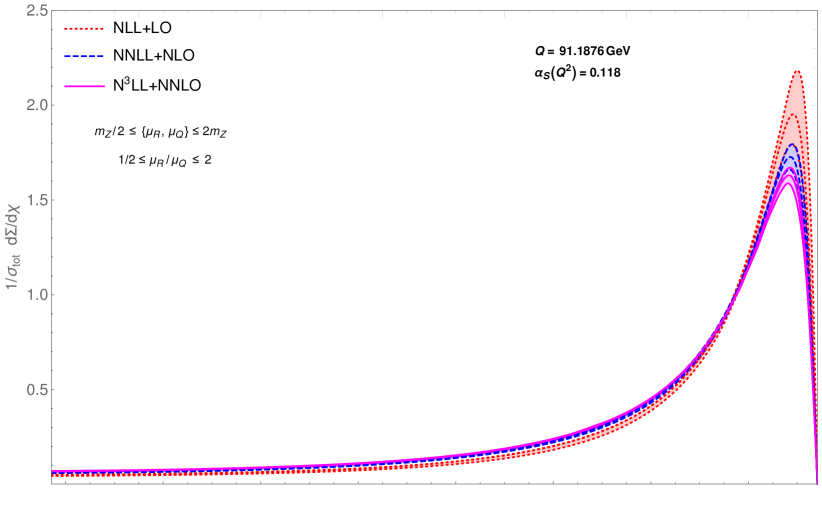
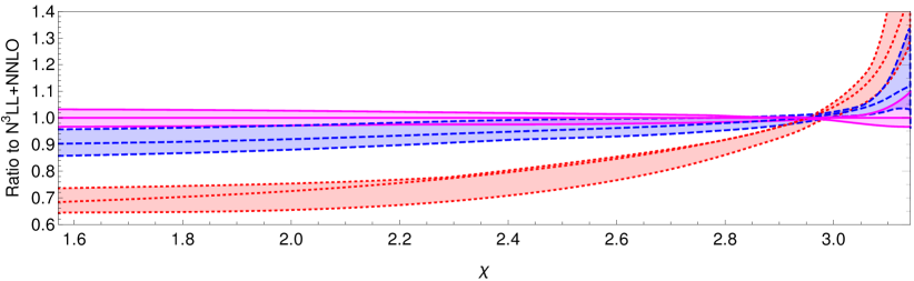
Figure 1: The EEC spectrum at $\sqrt{s}=91.1876$ GeV at various perturbative orders in QCD.

In Fig.1 we show the NLL+LO, NNLL+NLO and N³LL+NNLO predictions for the differential distribution of the EEC function. We observe that by increasing the logarithmic accuracy, the distribution becomes harder, i.e. the peak becomes smaller and broader and the low-$\chi$ tail becomes higher. This effect is not unexpected since at higher perturbative accuracy subleading effects from parton radiation are included.

In the lower panel of Fig. 1 we show the ratio of the predictions with respect to the N³LL+NNLO prediction at the central value of the scales $\mu_{R}=\mu_{Q}=Q$. We observe that the NLL+LO and NNLL+NLO scale dependence bands do overlap only for $\chi\gtrsim 2.9$ thus showing that the NLL+LO scale variation underestimates the true perturbative uncertainty in the wide region of $\chi\lesssim 2.9$. This is a typical feature of lower order perturbative predictions. In fact we point out that the NLL+LO prediction away from the back-to-back limit $\chi\to\pi$ is effectively a LO calculation. Conversely the NNLL+NLO and N³LL+NNLO scale dependence bands (slightly) overlap in the entire range considered of $\pi/2\leq\chi\leq\pi$ thus indicating that the scale variation at NNLL+NLO and (presumably) at N³LL+NNLO give a reasonably estimate of the true perturbative uncertainty. The N³LL+NNLO (NNLL+NLO) scale dependence is about $\pm 3\%$ ($\pm 5\%$) at $\chi\sim\pi/2$, then it constantly reduces for higher values of $\chi$ down to $\pm 0.5\%$ ($\pm 1\%$) for $\chi\sim 3$ (i.e. slightly before the peak) and it rapidly increases in the $\chi\to\pi$ limit. Overall going from NNLL+NLO to N³LL+NNLO the scale uncertainty reduces by about a factor of 2.

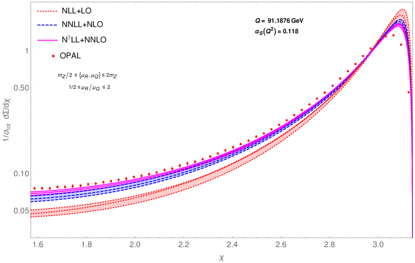
Figure 2: The EEC spectrum at $\sqrt{s}=91.1876$ GeV at various perturbative orders, compared with LEP data from the OPAL Collaboration [24].

Finally, in Fig. 2 we compare our perturbative predictions with the experimental EEC distribution measured by the OPAL Collaboration at LEP [24]. The perturbative scales are varied as in Fig. 1. We note that, by increasing the perturbative accuracy, the agreement with the experimental data improves, as expected. However, the N³LL+NNLO scale uncertainty band is definitively below the experimental distribution in the peak region and above it in the tail region. This discrepancy calls for an explicit and consistent inclusion of non-perturbative effects of parton hadronization.

7 Conclusions

In conclusion, in this paper we have presented the implementation of the QCD impact-parameter resummation formalism for the Energy-Energy-Correlation (EEC) distribution in the back-to-back region up to next-to-next-to-next-to-leading logarithmic (N³LL) accuracy. Away from the back-to-back region, we consistently combine resummed predictions with the known fixed-order results up to next-to-next-to-leading order (NNLO).

By expanding our QCD resummation formula up to second order in $\alpha_{S}$ and comparing the result with an exact QCD computation of the same order [17], we have been able to extract the NNLO coefficient of hard-virtual factor $H_{2}$. The latter was the last missing piece for reaching the (full) next-to-next-to-leading logarithmic (NNLL) accuracy in QCD. We have also been able to determine analytically the second-order remainder function, which is relevant outside the back-to-back region.

By extending the expansion of the resummation formula up to $\mathcal{O}(\alpha_{S}^{3})$ and comparing with an analytic computation in the Soft-Collinear Effective Theory (SCET) in the back-to-back region [12], we have also been able to determine the N³LO coefficients of the hard-virtual factor and of the of single logarithmic function of the Sudakov form factor $H_{3}$ and $B_{3}$. This allowed us for a complete resummation of the EEC function in the back-to-back region at full N³LL in QCD. By subtracting the $\mathcal{O}(\alpha_{S}^{3})$ part of the resummed distribution from a third-order numerical computation of the EEC in QCD in the full angular range ($0<\chi<\pi$) [9], we have also been able to estimate the NNLO (i.e. $\mathcal{O}(\alpha_{S}^{3})$) remainder function.

We have performed an independent variation of the renormalization scale $\mu_{R}$ and the resummation scale $\mu_{Q}$ as a way to estimate the perturbative theoretical error. The scale variation band at N³LL+NNLO is reduced by about a factor of 2 with respect to the previous order and it ranges from $\pm 3\%$ at $\chi\sim\pi/2$ down to $\pm 0.2\%$ for $\chi\sim 3$ and then increase again for $\chi\gtrsim 3$.

In the framework of a pure perturbative calculation by going from NNLL+NLO to the N³LL+NNLO accuracy, we find reasonably small corrections indicating a good convergence of the perturbative expansion.

Finally, we have compared our perturbative predictions to the EEC distribution measured by the OPAL Collaboration at the LEP collider at the $Z^{0}$ peak. Increasing the perturbative accuracy improves the compatibility of the theoretical predictions with the experimental data. However, there is still a substantial discrepancy between N³LL+NNLO prediction and data calling for the explicit inclusion of non-perturbative (NP) hadronization effects.

A more detailed phenomenological analysis, together with the introduction of a consistent NP model, is left for a future work.

Acknowledgments

We would like to thank Gabor Somogyi for providing us the numerical results of Ref. [9].

References

- [1] S. Catani, L. Trentadue, G. Turnock and B. R. Webber, “Resummation of large logarithms in e+ e- event shape distributions,” Nucl. Phys. B 407 (1993), 3-42 doi:10.1016/0550-3213(93)90271-P
- [2] C. L. Basham, L. S. Brown, S. D. Ellis and S. T. Love, “Energy Correlations in electron - Positron Annihilation: Testing QCD,” Phys. Rev. Lett. 41 (1978), 1585 doi:10.1103/PhysRevLett.41.1585
- [3] J. C. Collins and D. E. Soper, “Back-To-Back Jets in QCD,” Nucl. Phys. B 193 (1981), 381 [erratum: Nucl. Phys. B 213 (1983), 545] doi:10.1016/0550-3213(81)90339-4
- [4] J. C. Collins and D. E. Soper, “Back-To-Back Jets: Fourier Transform from B to K-Transverse,” Nucl. Phys. B 197 (1982), 446-476 doi:10.1016/0550-3213(82)90453-9
- [5] J. C. Collins and D. E. Soper, “The Two Particle Inclusive Cross-section in Annihilation at PETRA, PEP and LEP Energies,” Nucl. Phys. B 284 (1987), 253-270 doi:10.1016/0550-3213(87)90035-6
- [6] J. Kodaira and L. Trentadue, “Summing Soft Emission in QCD,” Phys. Lett. B 112 (1982), 66 doi:10.1016/0370-2693(82)90907-8.
- [7] J. Kodaira and L. Trentadue, “Single Logarithm Effects in electron-Positron Annihilation,” Phys. Lett. B 123 (1983), 335-338 doi:10.1016/0370-2693(83)91213-3
- [8] D. de Florian and M. Grazzini, “The Back-to-back region in e+ e- energy-energy correlation,” Nucl. Phys. B 704 (2005), 387-403 doi:10.1016/j.nuclphysb.2004.10.051 [arXiv:hep-ph/0407241 [hep-ph]].
- [9] Z. Tulipánt, A. Kardos and G. Somogyi, “Energy–energy correlation in electron–positron annihilation at NNLL + NNLO accuracy,” Eur. Phys. J. C 77 (2017) no.11, 749 doi:10.1140/epjc/s10052-017-5320-9 [arXiv:1708.04093 [hep-ph]].
- [10] A. Kardos, S. Kluth, G. Somogyi, Z. Tulipánt and A. Verbytskyi, “Precise determination of from a global fit of energy–energy correlation to NNLO+NNLL predictions,” Eur. Phys. J. C 78 (2018) no.6, 498 doi:10.1140/epjc/s10052-018-5963-1 [arXiv:1804.09146 [hep-ph]].
- [11] I. Moult and H. X. Zhu, “Simplicity from Recoil: The Three-Loop Soft Function and Factorization for the Energy-Energy Correlation,” JHEP 08 (2018), 160 doi:10.1007/JHEP08(2018)160 [arXiv:1801.02627 [hep-ph]].
- [12] M. A. Ebert, B. Mistlberger and G. Vita, “The Energy-Energy Correlation in the back-to-back limit at N3LO and N3LL’,” JHEP 08 (2021), 022 doi:10.1007/JHEP08(2021)022 [arXiv:2012.07859 [hep-ph]].
- [13] C. Duhr, B. Mistlberger and G. Vita, “Four-Loop Rapidity Anomalous Dimension and Event Shapes to Fourth Logarithmic Order,” Phys. Rev. Lett. 129 (2022) no.16, 162001 doi:10.1103/PhysRevLett.129.162001 [arXiv:2205.02242 [hep-ph]].
- [14] L. J. Dixon, I. Moult and H. X. Zhu, “Collinear limit of the energy-energy correlator,” Phys. Rev. D 100 (2019) no.1, 014009 doi:10.1103/PhysRevD.100.014009 [arXiv:1905.01310 [hep-ph]].
- [15] D. G. Richards, W. J. Stirling and S. D. Ellis, “Second Order Corrections to the Energy-energy Correlation Function in Quantum Chromodynamics,” Phys. Lett. B 119 (1982), 193-197 doi:10.1016/0370-2693(82)90275-1
- [16] D. G. Richards, W. J. Stirling and S. D. Ellis, “Energy-energy Correlations to Second Order in Quantum Chromodynamics,” Nucl. Phys. B 229 (1983), 317-346 doi:10.1016/0550-3213(83)90335-8
- [17] L. J. Dixon, M. X. Luo, V. Shtabovenko, T. Z. Yang and H. X. Zhu, “Analytical Computation of Energy-Energy Correlation at Next-to-Leading Order in QCD,” Phys. Rev. Lett. 120 (2018) no.10, 102001 doi:10.1103/PhysRevLett.120.102001 [arXiv:1801.03219 [hep-ph]].
- [18] V. Del Duca, C. Duhr, A. Kardos, G. Somogyi and Z. Trócsányi, “Three-Jet Production in Electron-Positron Collisions at Next-to-Next-to-Leading Order Accuracy,” Phys. Rev. Lett. 117 (2016) no.15, 152004 doi:10.1103/PhysRevLett.117.152004 [arXiv:1603.08927 [hep-ph]].
- [19] V. Del Duca, C. Duhr, A. Kardos, G. Somogyi, Z. Szőr, Z. Trócsányi and Z. Tulipánt, “Jet production in the CoLoRFulNNLO method: event shapes in electron-positron collisions,” Phys. Rev. D 94 (2016) no.7, 074019 doi:10.1103/PhysRevD.94.074019 [arXiv:1606.03453 [hep-ph]].
- [20] G. Bozzi, S. Catani, D. de Florian and M. Grazzini, “Transverse-momentum resummation and the spectrum of the Higgs boson at the LHC,” Nucl. Phys. B 737 (2006), 73-120 doi:10.1016/j.nuclphysb.2005.12.022 [arXiv:hep-ph/0508068 [hep-ph]].
- [21] G. Parisi and R. Petronzio, “Small Transverse Momentum Distributions in Hard Processes,” Nucl. Phys. B 154 (1979), 427-440 doi:10.1016/0550-3213(79)90040-3
- [22] J. C. Collins, D. E. Soper and G. F. Sterman, “Transverse Momentum Distribution in Drell-Yan Pair and W and Z Boson Production,” Nucl. Phys. B 250 (1985), 199-224 doi:10.1016/0550-3213(85)90479-1
- [23] S. Catani, D. de Florian and M. Grazzini, “Universality of nonleading logarithmic contributions in transverse momentum distributions,” Nucl. Phys. B 596 (2001), 299-312 doi:10.1016/S0550-3213(00)00617-9 [arXiv:hep-ph/0008184 [hep-ph]].
- [24] P. D. Acton et al. [OPAL], “A Determination of alpha-s (M (Z0)) at LEP using resummed QCD calculations,” Z. Phys. C 59 (1993), 1-20 doi:10.1007/BF01555834
- [25] S. G. Gorishnii, A. L. Kataev and S. A. Larin, “The -corrections to and in QCD,” Phys. Lett. B 259 (1991), 144-150 doi:10.1016/0370-2693(91)90149-K.
- [26] L. R. Surguladze and M. A. Samuel, “Total hadronic cross-section in e+ e- annihilation at the four loop level of perturbative QCD,” Phys. Rev. Lett. 66 (1991), 560-563 [erratum: Phys. Rev. Lett. 66 (1991), 2416] doi:10.1103/PhysRevLett.66.560
- [27] S. Catani, M. L. Mangano, P. Nason and L. Trentadue, “The Resummation of soft gluons in hadronic collisions,” Nucl. Phys. B 478 (1996), 273-310 doi:10.1016/0550-3213(96)00399-9 [arXiv:hep-ph/9604351 [hep-ph]].
- [28] E. Laenen, G. F. Sterman and W. Vogelsang, “Higher order QCD corrections in prompt photon production,” Phys. Rev. Lett. 84 (2000), 4296-4299 doi:10.1103/PhysRevLett.84.4296 [arXiv:hep-ph/0002078 [hep-ph]].
- [29] A. Kulesza, G. F. Sterman and W. Vogelsang, “Joint resummation in electroweak boson production,” Phys. Rev. D 66 (2002), 014011 doi:10.1103/PhysRevD.66.014011 [arXiv:hep-ph/0202251 [hep-ph]].
- [30] U. G. Aglietti, “Winter model in the quasi-continuum limit,” Int. J. Mod. Phys. A 35 (2020) no.06, 2050026 doi:10.1142/S0217751X20500268 [arXiv:1903.05051 [quant-ph]].
- [31] U. G. Aglietti and A. Cubeddu, “Winter (or -shell) model at small and intermediate volumes,” Annals Phys. 444 (2022), 169047 doi:10.1016/j.aop.2022.169047 [arXiv:2202.07616 [quant-ph]].
- [32] S. Camarda, L. Cieri and G. Ferrera, “Drell–Yan lepton-pair production: qT resummation at N4LL accuracy,” Phys. Lett. B 845 (2023), 138125 doi:10.1016/j.physletb.2023.138125 [arXiv:2303.12781 [hep-ph]].
- [33] J. Kodaira and L. Trentadue, “SOFT GLUON EFFECTS IN PERTURBATIVE QUANTUM CHROMODYNAMICS,” SLAC-PUB-2934.
- [34] O. V. Tarasov, A. A. Vladimirov and A. Y. Zharkov, “The Gell-Mann-Low Function of QCD in the Three Loop Approximation,” Phys. Lett. B 93 (1980), 429-432 doi:10.1016/0370-2693(80)90358-5
- [35] S. A. Larin and J. A. M. Vermaseren, “The Three loop QCD Beta function and anomalous dimensions,” Phys. Lett. B 303 (1993), 334-336 doi:10.1016/0370-2693(93)91441-O [arXiv:hep-ph/9302208 [hep-ph]].
- [36] T. van Ritbergen, J. A. M. Vermaseren and S. A. Larin, “The Four loop beta function in quantum chromodynamics,” Phys. Lett. B 400 (1997), 379-384 doi:10.1016/S0370-2693(97)00370-5 [arXiv:hep-ph/9701390 [hep-ph]].
- [37] M. Czakon, “The Four-loop QCD beta-function and anomalous dimensions,” Nucl. Phys. B 710 (2005), 485-498 doi:10.1016/j.nuclphysb.2005.01.012 [arXiv:hep-ph/0411261 [hep-ph]].
- [38] S. Moch, J. A. M. Vermaseren and A. Vogt, “The Three loop splitting functions in QCD: The Nonsinglet case,” Nucl. Phys. B 688 (2004), 101-134 doi:10.1016/j.nuclphysb.2004.03.030 [arXiv:hep-ph/0403192 [hep-ph]].
- [39] T. Becher and M. Neubert,“Drell-Yan Production at Small , Transverse Parton Distributions and the Collinear Anomaly,” Eur. Phys. J. C 71 (2011), 1665 doi:10.1140/epjc/s10052-011-1665-7 [arXiv:1007.4005 [hep-ph]].
- [40] S. Moch, B. Ruijl, T. Ueda, J. A. M. Vermaseren and A. Vogt, “On quartic colour factors in splitting functions and the gluon cusp anomalous dimension,” Phys. Lett. B 782 (2018), 627-632 doi:10.1016/j.physletb.2018.06.017 [arXiv:1805.09638 [hep-ph]].
- [41] A. von Manteuffel, E. Panzer and R. M. Schabinger, “Cusp and collinear anomalous dimensions in four-loop QCD from form factors,” Phys. Rev. Lett. 124 (2020) no.16, 162001 doi:10.1103/PhysRevLett.124.162001 [arXiv:2002.04617 [hep-ph]].
- [42] Y. Li and H. X. Zhu, “Bootstrapping Rapidity Anomalous Dimensions for Transverse-Momentum Resummation,” Phys. Rev. Lett. 118 (2017) no.2, 022004 doi:10.1103/PhysRevLett.118.022004 [arXiv:1604.01404 [hep-ph]].
- [43] J. Kodaira and L. Trentadue, “CAN SOFT GLUON EFFECTS BE MEASURED IN ELECTRON - POSITRON ANNIHILATION?,” Prog. Theor. Phys. 69 (1983), 693 doi:10.1143/PTP.69.693
- [44] R. Fiore, A. Quartarolo and L. Trentadue, “Energy-energy correlation for Theta — 180-degrees at LEP,” Phys. Lett. B 294 (1992), 431-435 doi:10.1016/0370-2693(92)91545-K
- [45] Y. L. Dokshitzer, G. Marchesini and B. R. Webber, “Nonperturbative effects in the energy energy correlation,” JHEP 07 (1999), 012 doi:10.1088/1126-6708/1999/07/012 [arXiv:hep-ph/9905339 [hep-ph]].