Chance-Constrained Control for Safe Spacecraft Autonomy:
Convex Programming Approach

Abstract

This paper presents a robust path-planning framework for safe spacecraft autonomy under uncertainty and develops a computationally tractable formulation based on convex programming. We utilize chance-constrained control to formulate the problem. It provides a mathematical framework to solve for a sequence of control policies that minimizes a probabilistic cost under probabilistic constraints with a user-defined confidence level (e.g., safety with 99.9% confidence). The framework enables the planner to directly control state distributions under operational uncertainties while ensuring the vehicle safety. This paper rigorously formulates the safe autonomy problem, gathers and extends techniques in literature to accommodate key cost/constraint functions that often arise in spacecraft path planning, and develops a tractable solution method. The presented framework is demonstrated via two representative numerical examples: safe autonomous rendezvous and orbit maintenance in cislunar space, both under uncertainties due to navigation error from Kalman filter, execution error via Gates model, and imperfect force models.

I Introduction

Safety is crucial in spacecraft autonomy. As any space vehicles must operate under various operational uncertainties, safety assurance under such uncertainties is prerequisite for any autonomous guidance navigation control (GNC) algorithms to be deployed on real-world space vehicles. Notable uncertainties in spacecraft GNC include navigation (estimation) error, maneuver execution error, and imperfect force models. It is a challenging task to ensure the safety of autonomous vehicles under such uncertainties with severe constraints in space operations, such as the limited onboard computation, communication bandwidth, and stringent safety constraints (e.g., keep-out zone, approach cone, tube/box constraints about nominal trajectories) [1].

To address the challenge, this paper leverages recent advances in chance-constrained control [2, 3, 4]. Chance-constrained control is a class of stochastic control that seeks a sequence of control policies that minimizes a probabilistic cost while imposing probabilistic constraints with a user-defined confidence level. A chance constraint is defined as:

$$\begin{aligned} \mathbb{P}\left[\mathrm{safe}\right]\geq 1-\varepsilon,\quad\end{aligned}$$ (1)

where $\varepsilon$ is a risk bound (e.g., $\varepsilon=0.01$ for $99\%$ confidence). Chance-constrained approaches directly control and impose safety constraints on state distributions under uncertainty, which is in sharp contrast to conventional GNC algorithms, such as those based on Gauss equations [5], convex programming [6, 7], predictor-corrector [8, 9], sliding-mode control [10], and model predictive control (MPC) [11, 12]. A key advantage over other robust control approaches, such as robust MPC [13, 14, 15, 16], lies in its ability to handle unbounded distributions, which are common in spacecraft GNC, e.g., Gaussian-distributed state estimate from a Kalman filter.

Fig. 1 illustrates the safe autonomy framework envisioned in this study. In this framework, a chunk of chance-constrained control policies, $\pi_{1:N}$ ($N$: planning horizon), are computed on ground via convex programming, infrequently uploaded to spacecraft, and run on-board to calculate maneuvers every time a new state estimate becomes available via filtering. Maneuvers derived from the policies are safe by design under uncertainties that are modeled in the planner.

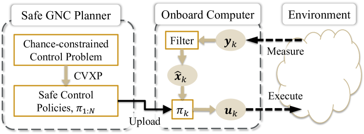
Figure 1: Safe autonomy framework based on chance-constrained control

The main contributions of this paper are threefold. First, this paper rigorously formulates the safe spacecraft autonomy concept envisioned in Fig. 1 as an output-feedback chance-constrained control problem. Second, we extend techniques in literature to incorporate notable cost function and constraints in spacecraft GNC and to exploit the Markovian property of the system. Third, this paper demonstrates the autonomy framework via two representative scenarios: safe autonomous rendezvous and station-keeping on a cislunar near rectilinear halo orbit (NRHO).

Notation

$\mathbb{Z}_{0}^{N}$ denotes the set of integers from $0$ to $N$. $\lVert\cdot\rVert_{p}$ denotes $l_{p}$ norm for a vector. For a matrix $A$, $\lVert A\rVert_{2}$ is its spectral norm while $\lambda_{\max}(A)(=\lVert A\rVert_{2}^{2})$ is its maximum eigenvalue. For a matrix $A\succeq 0$, $A^{1/2}$ is lower-triangular and satisfies $A=A^{1/2}[A^{1/2}]^{\top}$. $\mathbb{P}\left[\cdot\right]$, $\mathbb{E}{[\cdot]}$, and $\mathrm{Cov}[\cdot]$ are probability, expectation, and covariance operators.

II Orbital Mechanics under Control

II-A Generic Formulation

Let $\bm{x}\in\mathbb{R}^{n_{x}}$ be the spacecraft orbital state and $\bm{u}\in\mathbb{R}^{n_{u}}$ be the control input. In general, spacecraft orbital dynamics under control are expressed as a control-affine system:

$$\begin{aligned} \dot{\bm{x}}=&\bm{f}(\bm{x},\bm{u},t)=\bm{f}_{0}(\bm{x},t)+B\bm{u},\quad B=\begin{bmatrix}0_{n_{u}\times n_{u}}\\ I_{n_{u}}\end{bmatrix}\end{aligned}$$ (2)

where $\bm{f}_{0}(\cdot)$ represents orbital dynamics under no control. The control input $\bm{u}$ may model impulsive maneuvers (delta-V) or continuous acceleration. We characterize $\bm{u}(t)$ by a finite number of control inputs $\bm{u_{k}},k\in\mathbb{Z}_{0}^{N-1}$ as:

$$\begin{aligned} \bm{u}(t)=\begin{cases}\sum_{k=0}^{N-1}\bm{u}_{k}\delta(t-t_{k})&\text{(impulsive)}\\ \bm{u}_{k},\quad\forall t\in[t_{k},t_{k+1})&\text{(continuous)}\end{cases}\end{aligned}$$ (3)

where $\delta(\cdot)$ is the Dirac delta function, and the zero-order-hold (ZOH) is assumed for continuous control.

II-B Specific Formulations

Appropriate equations of motion (EoMs) to use depend on the orbital regime and operation scenario. Let us review some popular forms of $\bm{f}_{0}(\cdot)$ with underlying assumptions.

II-B1 Perturbed 2BP

The perturbed two-body problem (2BP) expressed in Cartesian coordinates is a common dynamical system in spacecraft GNC. The state is defined as $\bm{x}=[\bm{r}^{\top},\bm{v}^{\top}]^{\top}$, where $\bm{r},\bm{v}$ are the spacecraft position and velocity, and $\bm{f}_{0}(\cdot)$ is given by [17]:

$$\begin{aligned} \bm{f}_{0}(\bm{x},t)=\begin{bmatrix}\bm{v}\\ -\frac{\mu}{\lVert\bm{r}\rVert_{2}^{3}}\bm{r}\end{bmatrix}+B\bm{a}(\bm{x},t)\end{aligned}$$ (4)

where $\mu$ is the gravitational parameter of the body, and $\bm{a}$ is perturbing acceleration due to the surrounding environment.

II-B2 CWH equation

Clohessy-Wiltshire Hill (CWH) equation approximates Eq. 4 to model orbital motion in proximity of another object (called chief satellite) . CWH equation is derived with assumptions that (i) the chief and our spacecraft is sufficiently close, and (ii) the chief orbit is circular about the gravitational body. The state is defined as $\bm{x}=[\bm{r}^{\top},\bm{v}^{\top}]^{\top}$, where $\bm{r},\bm{v}\in\mathbb{R}^{3}$ are the spacecraft position and velocity in a rotating frame that rotates with the chief orbit about the gravitational body. $\bm{f}_{0}(\cdot)$ is given by [18]:

$$\begin{aligned} &\bm{f}_{0}(\bm{x},t)=A\bm{x}+B\bm{a}(\bm{x},t),\quad A=\begin{bmatrix}0_{3\times 3}&I_{3}\\ A_{21}&A_{22}\end{bmatrix},\\ &A_{21}=\begin{bmatrix}3n^{2}&0&0\\ 0&0&0\\ 0&0&-n^{2}\end{bmatrix},\quad A_{22}=\begin{bmatrix}0&2n&0\\ -2n&0&0\\ 0&0&0\end{bmatrix}\end{aligned}$$ (5)

where $n=\sqrt{{\mu}/{r_{0}^{3}}}$, and $r_{0}$ is the chief orbit radius.

II-B3 CR3BP

Circular Restricted Three-Body Problem (CR3BP) is the simplest possible expression of the three-body problem. It assumes that two massive bodies with gravitational parameters $\mu_{1}$ and $\mu_{2}$ are in a circular orbit about their barycenter. The state vector is defined as $\bm{x}=[\bm{r}^{\top},\bm{v}^{\top}]^{\top}$, where $\bm{r}=[x,y,z]^{\top}$ and $\bm{v}=[\dot{x},\dot{y},\dot{z}]^{\top}$ are non-dimensional spacecraft position and velocity in the rotating frame that rotates with the two massive bodies. $\bm{r}$ and $\bm{v}$ can be dimensionalized by multiplying the characteristic length $l_{*}$ and velocity $v_{*}$, where $l_{*}$ is the distance between the two massive bodies, $v_{*}=l_{*}/t_{*}$, and $t_{*}$ (characteristic time) is given by $t_{*}=\sqrt{l_{*}^{3}/(\mu_{1}+\mu_{2})}$. $\bm{f}_{0}(\cdot)$ is given by [19]:

$$\bm{f}_{0}(\bm{x},t)=\begin{bmatrix}\bm{v}\\ \bm{f}_{a}(\bm{x})\end{bmatrix}+B\bm{a}$$ (6)

$\bm{f}_{a}(\cdot)$ is given in Eq. 7, where $\mu=\mu_{2}/(\mu_{1}+\mu_{2})$, $r_{1}=\sqrt{(x+\mu)^{2}+y^{2}+z^{2}}$, and $r_{2}=\sqrt{(x-1+\mu)^{2}+y^{2}+z^{2}}$.

$$\bm{f}_{a}(\bm{x})=\begin{bmatrix}2\dot{y}+x-\frac{(1-\mu)(x+\mu)}{r_{1}^{3}}-\frac{\mu(x-1+\mu)}{r_{2}^{3}}\\ -2\dot{x}+y-\frac{(1-\mu)y}{r_{1}^{3}}-\frac{\mu y}{r_{2}^{3}}\\ \frac{-(1-\mu)z}{r_{1}^{3}}-\frac{\mu z}{r_{2}^{3}}\end{bmatrix}$$ (7)

III Chance-Constrained Control Problem

III-A Uncertainty Modeling

III-A1 Initial state dispersion

We model the distributions of $\hat{\bm{x}}$ (estimate of $\bm{x}$) and $\widetilde{\bm{x}}(=\bm{x}-\hat{\bm{x}})$ at $t_{0}$ via independent Gaussian distributions as

$$\hat{\bm{x}}_{0}^{-}\sim\mathcal{N}(\mskip 1.5mu\overline{\mskip-1.5mu{\bm{x}}\mskip-1.5mu}\mskip 1.5mu_{0},\hat{P}_{0^{-}}),\ \widetilde{\bm{x}}_{0}\sim\mathcal{N}(0,\widetilde{P}_{0^{-}}),$$ (8)

which implies $\bm{x}_{0}=\hat{\bm{x}}_{0}^{-}+\widetilde{\bm{x}}_{0}\sim\mathcal{N}(\mskip 1.5mu\overline{\mskip-1.5mu{\bm{x}}\mskip-1.5mu}\mskip 1.5mu_{0},\hat{P}_{0^{-}}+\widetilde{P}_{0})$.

III-A2 Maneuver execution error

The Gates model [20] is a common approach to execution error modeling. For a given $\bm{u}_{k}$, it models the control error, $\widetilde{\bm{u}}_{k}$, as [21, 22]:

$$\begin{aligned} &\widetilde{\bm{u}}(t)=\begin{cases}\sum_{k=0}^{N-1}\widetilde{\bm{u}}_{k}\delta(t-t_{k})&\text{(impulsive)}\\ \widetilde{\bm{u}}_{k},\forall t\in[t_{k},t_{k+1})&\text{(continuous)}\end{cases},\\ &\widetilde{\bm{u}}_{k}=G_{\mathrm{exe}}(\bm{u}_{k})\bm{w}_{\mathrm{exe},k},\quad\bm{w}_{\mathrm{exe},k}\sim\mathcal{N}(0,I_{3}),\\ &G_{\mathrm{exe}}(\bm{u}_{k})=T(\bm{u}_{k})P_{\mathrm{gates}}^{1/2}(\bm{u}_{k})\end{aligned}$$ (9)

where $\bm{w}_{\mathrm{exe},k}$ are i.i.d. standard Gaussian vectors, and

$$\begin{aligned} &P_{\mathrm{gates}}(\cdot)=\mathrm{diag}(\sigma_{p}^{2},\sigma_{p}^{2},\sigma_{m}^{2}),\ T(\cdot)=\begin{bmatrix}\hat{\bm{S}}&\hat{\bm{E}}&\hat{\bm{Z}}\end{bmatrix},\\ &\hat{\bm{Z}}=\frac{\bm{u}_{k}}{\lVert\bm{u}_{k}\rVert_{2}},\ \hat{\bm{E}}=\frac{[0,0,1]^{\top}\times\hat{\bm{Z}}}{\lVert[0,0,1]^{\top}\times\hat{\bm{Z}}\rVert_{2}},\ \hat{\bm{S}}=\hat{\bm{E}}\times\hat{\bm{Z}}\end{aligned}$$ (10)

Here, $\sigma_{p}^{2}=\sigma_{3}^{2}+\sigma_{4}^{2}\lVert\bm{u}_{k}\rVert_{2}^{2}$ and $\sigma_{m}^{2}=\sigma_{1}^{2}+\sigma_{2}^{2}\lVert\bm{u}_{k}\rVert_{2}^{2}$. Note that $\{\sigma_{1},\sigma_{2}\}$ are {fixed, proportional} magnitude errors while $\{\sigma_{3},\sigma_{4}\}$ are {fixed, proportional} pointing errors.

III-A3 Stochastic acceleration

Stochastic acceleration due to imperfect force modeling can be naturally modeled by a Brownian motion: $G(\bm{x})\mathrm{d}\bm{w}(t)$, where $G(\cdot)$ is the intensity of disturbances; $\mathrm{d}\bm{w}(t)$ is a standard Brownian motion vector, i.e., $\mathbb{E}{[\mathrm{d}\bm{w}]}=0_{3}$ and $\mathbb{E}{[\mathrm{d}\bm{w}(t)\mathrm{d}\bm{w}^{\top}(t)]}=I_{3}\mathrm{d}t$.

III-A4 Navigation uncertainty

In essence, navigation is a filtering process with discrete observations, modeled as:

$$\begin{aligned} \bm{y}_{k}=&\bm{f}_{\mathrm{obs}}(\bm{x}_{k})+G_{\mathrm{obs}}(\bm{x}_{k})\bm{w}_{\mathrm{obs},k},\end{aligned}$$ (11)

where $\bm{f}_{\mathrm{obs}}(\cdot)$ and $G_{\mathrm{obs}}(\cdot)$ are the measurement function and noise intensity, respectively; $\bm{w}_{\mathrm{obs},k}\in\mathbb{R}^{n_{y}}$ is an i.i.d. standard Gaussian vector. A navigation solution at time $t_{k}$, denoted by $\hat{\bm{x}}_{k}$, is expressed in terms of its probability density function (pdf) conditioned on all the past measurements $\bm{y}_{1:k}$:

$$\begin{aligned} &\hat{\bm{x}}_{k}\sim f_{\mathrm{pdf}}(\bm{x}_{k}|\bm{y}_{1:k})=\mathcal{F}(\bm{x}_{k},\bm{y}_{1:k})\end{aligned}$$ (12)

where $\mathcal{F}(\cdot)$ denotes the filtering process. Filtering typically utilizes the innovation process $\widetilde{\bm{y}}_{k}^{-}$, defined as:

$$\begin{aligned} \widetilde{\bm{y}}_{k}^{-}=\bm{y}_{k}-\bm{f}_{\mathrm{obs}}(\hat{\bm{x}}_{k}^{-}).\end{aligned}$$ (13)

III-A5 Nonlinear Stochastic System

The evolution of stochastic state is naturally modeled by nonlinear stochastic differential equation (SDE) as:

$$\begin{aligned} \mathrm{d}\bm{x}=&[\bm{f}(\bm{x},\bm{u},t)+B\widetilde{\bm{u}}]\mathrm{d}t+G(\bm{x})\mathrm{d}\bm{w}(t)\end{aligned}$$ (14)

III-B Orbit Control under Uncertainty

III-B1 Cost Function

In stochastic settings, the classical form $J=\int_{t_{0}}^{t_{f}}L(\bm{u})\mathrm{d}t$ ($L$: Lagrangian cost) is not well defined because $\bm{u}$, hence $L(\cdot)$, may be now stochastic. Instead, we minimize the integral of the $p$-quantile of $L(\cdot)$, i.e.,

$$\begin{aligned} J=\int_{t_{0}}^{t_{f}}Q_{L(\bm{u})}(p)\mathrm{d}t\end{aligned}$$ (15)

where $Q_{X}(p)$ is the quantile function of a random variable $X$ evaluated at probability $p$, formally defined as:

$$Q_{X}(p)=\min\{a\in\mathbb{R}\mid\mathbb{P}\left[X\leq a\right]\geq p\}.$$ (16)

This paper is focused on minimizing $\Delta V_{99}$, i.e., $99\%$ quantile of fuel cost, corresponding to $L(\cdot)=\lVert\bm{u}\rVert_{2}$ with $p=0.99$.

III-B2 Path chance constraints

As our state and control are subject to uncertainty, constraints are not deterministic anymore and need to be treated probabilistically. We use chance constraints Eq. 1 to replace classical path constraints.

This paper is focused on chance constraints imposed at discrete epochs, although there are studies that extend the concept to continuous-time chance constraints [23].

A simple yet versatile form of state chance constraints is an intersection of hyperplane constraints:

$$\begin{aligned} \mathbb{P}\left[\bigwedge_{j}\bm{a}_{j}^{\top}\bm{x}_{k}+b_{j}\leq 0\right]\geq 1-\varepsilon_{x},\ k\in\mathbb{Z}_{0}^{N}\end{aligned}$$ (17)

which can conservatively represent any convex feasible regions, including box constraints about a reference trajectory.

If a tube-like constraint about a reference trajectory is preferred over box constraints, we could also consider

$$\begin{aligned} \mathbb{P}\left[\lVert H(\bm{x}_{k}-\bm{x}_{k}^{*})\rVert_{2}\leq d_{\max}\right]\geq 1-\varepsilon_{x},\ k\in\mathbb{Z}_{0}^{N}\end{aligned}$$ (18)

where $H\in\mathbb{R}^{n_{h}\times n_{x}}$ extracts specific elements from $\bm{x}$ (e.g., $H=[I_{3},0_{3\times 3}]$ to extract position), $\bm{x}_{k}^{*}$ is the reference state at the epoch, and $d_{\max}$ is the state deviation bound.

Let us then consider control chance constraints. A common control constraint is the magnitude constraint, $\lVert\bm{u}_{k}\rVert_{2}\leq u_{\max}$, whose chance-constraint counterpart is given by:

$$\begin{aligned} \mathbb{P}\left[\lVert\bm{u}_{k}\rVert_{2}\leq u_{\max}\right]\geq 1-\varepsilon_{u},\ k\in\mathbb{Z}_{0}^{N-1}\end{aligned}$$ (19)

In addition, constraints on control change rate may be crucial when the time for an attitude maneuver can be a bottleneck to thrust direction change; such a constraint is given by:

$$\begin{aligned} \mathbb{P}\left[\lVert\bm{u}_{k+1}-\bm{u}_{k}\rVert_{2}\leq\Delta u_{\max}\right]\geq 1-\varepsilon_{u},\ k\in\mathbb{Z}_{0}^{N-2}\end{aligned}$$ (20)

III-B3 Distributional terminal constraints

A natural extension of deterministic terminal constraints would ensure the spacecraft to nominally arrive at the target $\bm{x}_{f}$ within some prescribed accuracy represented by the final covariance $P_{f}$:

$$\begin{aligned} \mathbb{E}[{\bm{x}}_{N}]-\bm{x}_{f}=0,\quad P_{N}\preceq P_{f}\end{aligned}$$ (21)

where $P_{N}$ denotes the covariance of the $N$-th state.

III-B4 State-triggered chance constraints

State-triggered constraints may arise in many spacecraft GNC problems, especially when we have multiple phases in a mission. In deterministic form, a state-triggered constraint (STC) is expressed as: if $g_{\mathrm{stc}}(\bm{x},\bm{u})<0$, then $c_{\mathrm{stc}}(\bm{x},\bm{u})\leq 0$. This STC is shown in [24] to be logically equivalent to

$$h_{\mathrm{stc}}(\bm{x},\bm{u})\triangleq-\min\{g_{\mathrm{stc}}(\bm{x},\bm{u}),0\}\cdot c_{\mathrm{stc}}(\bm{x},\bm{u})\leq 0$$ (22)

The equivalence can be understood by noting that Eq. 22 implies that, if $g_{\mathrm{stc}}(\cdot)<0$, then $h_{\mathrm{stc}}(\cdot)=-g_{\mathrm{stc}}(\cdot)c_{\mathrm{stc}}(\cdot)\leq 0$, and hence $c_{\mathrm{stc}}(\cdot)\leq 0$; on the other hand, if $g_{\mathrm{stc}}(\cdot)\geq 0$, then $h_{\mathrm{stc}}(\cdot)=0$ regardless of the value of $c_{\mathrm{stc}}(\cdot)$.

An extension of this concept to a chance constraint with risk level $\epsilon$ can be expressed as:

$$\text{if }\mathbb{E}[g(\bm{x},\bm{u})]<0,\text{ then }\mathbb{P}\left[c(\bm{x},\bm{u})\leq 0\right]\geq 1-\epsilon$$ (23)

which means that $\mathbb{P}\left[c(\bm{x},\bm{u})\leq 0\right]\geq 1-\epsilon$ is imposed when the trigger condition $g(\bm{x},\bm{u})<0$ is satisfied in expectation.

In this paper, we consider an approach-cone constraint that is triggered when our satellite is near the origin (e.g., chief satellite). An approach cone can be represented by a second-order cone $\lVert A_{\mathrm{cone}}\bm{r}\rVert_{2}\leq\bm{b}_{\mathrm{cone}}^{\top}\bm{r}$; for instance, if the satellite is allowed to approach the chief from ${+}y$ direction, $\sqrt{r_{x}^{2}+r_{z}^{2}}\leq r_{y}\tan{\theta_{\max}}$, where $\theta_{\max}$ is half of the cone angle. Thus, we can specialize Eq. 23 as follows:

$$\begin{aligned} &\text{if}&&\mathbb{E}\left[\lVert H_{r}\bm{x}_{k}\rVert_{2}\right]<r_{\mathrm{trigger}},\\ &\text{then}&&\mathbb{P}\left[\lVert A_{\mathrm{cone}}H_{r}\bm{x}_{k}\rVert_{2}\leq\bm{b}_{\mathrm{cone}}^{\top}H_{r}\bm{x}_{k}\right]\geq 1-\epsilon_{x}\end{aligned}$$ (24)

where $H_{r}\in\mathbb{R}^{3\times n_{x}}$ extracts the position vector from $\bm{x}$, and $r_{\mathrm{trigger}}$ is the critical radius about the origin.

III-B5 Control policy

Since spacecraft never has access to the perfect state knowledge, control policies must calculate maneuvers using imperfect navigation solutions from Eq. 12. We model the control policy generically as:

$$\begin{aligned} \bm{u}_{k}=\pi_{k}(\hat{\bm{x}}_{k};\Omega_{k}),\end{aligned}$$ (25)

where $\Omega_{k}$ is a set of parameters that parameterize $\pi_{k}$.

III-C Original Chance-Constrained Orbit Control Problem

Problem 1.

Find $\pi_{k}(\cdot),\ k\in\mathbb{Z}_{0}^{N-1}$ that minimize Eq. 15 while obeying the SDE Eq. 14 and satisfying the chance constraints Eqs. 17, 18, 19 and 20, terminal constraint Eq. 21, and state-triggered chance constraints Eq. 24 under control policies given by Eq. 25 with the state estimates Eq. 12.

IV Solution Method via Convex Programming

IV-A Linear State Statistics Dynamics

IV-A1 Linear, discrete-time system

Linearizing Eq. 14 about the reference state $\bm{x}^{*}(t)$ and control $\bm{u}^{*}(t)$, we have

$$\mathrm{d}\bm{x}=(A\bm{x}+B^{*}\bm{u}+\bm{c}+B^{*}\widetilde{\bm{u}}^{*})\mathrm{d}t+G^{*}\mathrm{d}\bm{w}(t),$$

$$A=\left({\partial\bm{f}}/{\partial\bm{x}}\right)^{*},\ \bm{c}=\left(\bm{f}-A\bm{x}-B\bm{u}\right)^{*}$$ (26)

where $(\cdot)^{*}$ indicates the evaluation at $\bm{x}^{*}(t),\bm{u}^{*}(t)$.

Integrating Eq. 26 over an interval $[t_{k},t_{k+1})$ yields

$$\begin{aligned} \bm{x}_{k+1}=A_{k}\bm{x}_{k}+B_{k}\bm{u}_{k}+\bm{c}_{k}+G_{\mathrm{exe},k}\bm{w}_{\mathrm{exe},k}+G_{k}\bm{w}_{k}\end{aligned}$$ (27)

where $\bm{w}_{\mathrm{exe},k}\sim\mathcal{N}(0,I_{n_{u}})$ and $\bm{w}_{k}\sim\mathcal{N}(0,I_{n_{x}})$. The system matrices $A_{k},B_{k},\bm{c}_{k},G_{\mathrm{exe},k}$ are given by:

$$A_{k}=\Phi(t_{k+1},t_{k}),$$

$$B_{k}=\begin{cases}A_{k}B^{*}(t_{k})&\text{(impulsive)}\\ A_{k}\int_{t_{k}}^{t_{k+1}}\Phi^{-1}(t,t_{k})B^{*}(t)\mathrm{d}t&\text{(continuous)}\end{cases},$$ (28)

$$\bm{c}_{k}=A_{k}\int_{t_{k}}^{t_{k+1}}\Phi^{-1}(t,t_{k})\bm{c}(t)\mathrm{d}t,\ G_{\mathrm{exe},k}=B_{k}G_{\mathrm{exe}}(\bm{u}_{k}^{*})$$

while $G_{k}$ is any matrix such that $G_{k}\bm{w}_{k}$ has covariance

$$\begin{aligned} A_{k}\left\{\int_{t_{k}}^{t_{k+1}}\Phi^{-1}(t,t_{k})G(t)[\Phi^{-1}(t,t_{k})G(t)]^{\top}\mathrm{d}t\right\}A_{k}^{\top}\end{aligned}$$

Note that $\Phi(t,t_{k})$ denotes a state transition matrix from $t_{k}$ to $t$, obtained by solving the ordinary differential equation:

$$\begin{aligned} \dot{\Phi}(t,t_{k})=A(t)\Phi(t,t_{k}),\quad\Phi(t_{k},t_{k})=I\end{aligned}$$ (29)

If $\bm{u}_{k}^{*}=0$, then $T(\bm{u}_{k}^{*})$ in Eq. 10 is undefined and so is $G_{\mathrm{exe}}(\bm{u}_{k}^{*})$; in such a case, we model it as $T(\bm{u}_{k}^{*})=I_{3}$.

IV-A2 Filtered state dynamics

We assume that the spacecraft is equipped with a Kalman filter to calculate navigation solutions onboard. Hence, Eq. 11 is approximated as:

$$\bm{y}_{k}=C_{k}\bm{x}_{k}+D_{k}\bm{w}_{\mathrm{obs},k}+\bm{c}_{\mathrm{obs},k},\ \mathrm{with}\ C_{k}=[{\partial\bm{f}_{\mathrm{obs}}}/{\partial\bm{x}}]^{*},$$

$$D_{k}=G_{\mathrm{obs}}(\bm{x}_{k}^{*}),\ \bm{c}_{\mathrm{obs},k}=\bm{f}_{\mathrm{obs}}(\bm{x}_{k}^{*})-C_{k}\bm{x}_{k}^{*}$$ (30)

Likewise, $\bm{f}_{\mathrm{obs}}(\hat{\bm{x}}_{k}^{-})\approx\bm{c}_{\mathrm{obs},k}+C_{k}\hat{\bm{x}}_{k}^{-}$, leading Eq. 13 to

$$\begin{aligned} \widetilde{\bm{y}}_{k}^{-}=\bm{y}_{k}-(\bm{c}_{\mathrm{obs},k}+C_{k}\hat{\bm{x}}_{k}^{-})=C_{k}\widetilde{\bm{x}}_{k}+D_{k}\bm{w}_{\mathrm{obs},k}\end{aligned}$$ (31)

whose distribution is derived as (with $\widetilde{P}_{k}\triangleq\mathrm{Cov}[\widetilde{\bm{x}}_{k}]$):

$$\begin{aligned} \widetilde{\bm{y}}_{k}^{-}\sim\mathcal{N}(0,P_{\widetilde{y}_{k}^{-}}),\ P_{\widetilde{y}_{k}^{-}}=C_{k}\widetilde{P}_{k}^{-}C_{k}^{\top}+D_{k}D_{k}^{\top}\end{aligned}$$ (32)

The Kalman filter sequentially updates the state estimate as:

$$\hat{\bm{x}}_{k}^{-} =A_{k-1}\hat{\bm{x}}_{k-1}+B_{k-1}\bm{u}_{k-1}+\bm{c}_{k-1}\quad(\mathrm{time\ update})$$

$$\hat{\bm{x}}_{k} =\hat{\bm{x}}_{k}^{-}+L_{k}\widetilde{\bm{y}}_{k}^{-}\quad(\mathrm{measurement\ update})$$ (33)

which can be combined to yield

$$\begin{aligned} \hat{\bm{x}}_{k+1}=A_{k}\hat{\bm{x}}_{k}+B_{k}\bm{u}_{k}+\bm{c}_{k}+L_{k+1}\widetilde{\bm{y}}_{k+1}^{-}\end{aligned}$$ (34)

where $\hat{\bm{x}}_{0}=\hat{\bm{x}}_{0}^{-}+L_{0}\widetilde{\bm{y}}_{0}^{-}$. Here, $L_{k}$ is the Kalman gain:

$$\begin{aligned} L_{k}=\widetilde{P}_{k}^{-}C_{k}^{\top}(C_{k}\widetilde{P}_{k}^{-}C_{k}^{\top}+D_{k}D_{k}^{\top})^{-1}\end{aligned}$$ (35)

which can be analytically calculated a priori in linear Kalman filter since $\widetilde{P}_{k}$ and $\widetilde{P}_{k}^{-}$ are also available a priori:

$$\widetilde{P}_{k}^{-} =A_{k-1}\widetilde{P}_{k-1}A_{k-1}^{\top}+G_{\mathrm{exe},k-1}G_{\mathrm{exe},k-1}^{\top}+G_{k-1}G_{k-1}^{\top}$$

$$\widetilde{P}_{k} =(I-L_{k}C_{k})\widetilde{P}_{k}^{-}(I-L_{k}C_{k})^{\top}+L_{k}D_{k}D_{k}^{\top}L_{k}^{\top}$$ (36)

IV-A3 Linear output-feedback control policy

We model the control policy Eq. 25 in a linear output feedback form as:

$$\begin{aligned} \bm{u}_{k}&=\mskip 1.5mu\overline{\mskip-1.5mu{\bm{u}}\mskip-1.5mu}\mskip 1.5mu_{k}+K_{k}\bm{z}_{k},\ k\in\mathbb{Z}_{0}^{N-1}\end{aligned}$$ (37)

where $\mskip 1.5mu\overline{\mskip-1.5mu{\bm{u}}\mskip-1.5mu}\mskip 1.5mu_{k}$ is a nominal control input, $K_{k}$ is a feedback gain matrix, and $\bm{z}_{k}$ is a stochastic process given by

$$\begin{aligned} \bm{z}_{k+1}=A_{k}\bm{z}_{k}+L_{k+1}\widetilde{\bm{y}}_{k+1}^{-},\quad\bm{z}_{0}=\hat{\bm{x}}_{0}-\mskip 1.5mu\overline{\mskip-1.5mu{\bm{x}}\mskip-1.5mu}\mskip 1.5mu_{0}.\end{aligned}$$ (38)

This approach, originally proposed by the author and collaborators in [25], exploits the system’s Markovian property.

IV-A4 State and control statistics

Let us first analytically derive the statistics—mean and covariance—of the state and control. We express Eq. 34 in a block-matrix form as:

$$\begin{aligned} &\begin{bmatrix}\hat{\bm{x}}_{0}\\ \hat{\bm{x}}_{1}\\ \hat{\bm{x}}_{2}\\ \vdots\end{bmatrix}=\begin{bmatrix}I_{n_{x}}\\ A_{0}\\ A_{1}A_{0}\\ \vdots\end{bmatrix}\hat{\bm{x}}_{0}^{-}+\begin{bmatrix}0&0&\\ B_{0}&0&\\ A_{1}B_{0}&B_{1}&\\ &&{\ddots}\end{bmatrix}\begin{bmatrix}\bm{u}_{0}\\ \bm{u}_{1}\\ \bm{u}_{2}\\ \vdots\end{bmatrix}+\\ &\begin{bmatrix}0&0&\\ I_{n_{x}}&0&\\ A_{1}&I_{n_{x}}&\\ &&{\ddots}\end{bmatrix}\begin{bmatrix}\bm{c}_{0}\\ \bm{c}_{1}\\ \bm{c}_{2}\\ \vdots\end{bmatrix}+\begin{bmatrix}L_{0}&0&\\ A_{0}L_{0}&L_{1}&\\ A_{1}A_{0}L_{0}&A_{1}L_{1}&\\ &&{\ddots}\end{bmatrix}\begin{bmatrix}\widetilde{\bm{y}}_{0}^{-}\\ \widetilde{\bm{y}}_{1}^{-}\\ \widetilde{\bm{y}}_{2}^{-}\\ \vdots\end{bmatrix}\end{aligned}$$

which can be expressed in a compact form as:

$$\begin{aligned} \hat{\bm{X}}=\mathbf{A}\hat{\bm{x}}_{0}^{-}+\mathbf{B}\bm{U}+\mathbf{C}+\mathbf{L}{\bm{Y}},\end{aligned}$$ (39)

where $\hat{\bm{X}}=[\hat{\bm{x}}_{0}^{\top},\hat{\bm{x}}_{1}^{\top},...,\hat{\bm{x}}_{N}^{\top}]^{\top}$, $\bm{U}=[\bm{u}_{0}^{\top},\bm{u}_{1}^{\top},...,\bm{u}_{N-1}^{\top}]^{\top}$, $\bm{Y}=[\widetilde{\bm{y}}_{0}^{-1^{\top}},\widetilde{\bm{y}}_{1}^{-1^{\top}},...,\widetilde{\bm{y}}_{N}^{-1^{\top}}]^{\top}$, and $\mathbf{A},\mathbf{B},\mathbf{C},\mathbf{L}$ are defined accordingly. See [3, 4] on this construction. Here, we define matrices $E_{x_{k}}$ ($E_{u_{k}}$) to extract $\bm{x}_{k}$ ($\bm{u}_{k}$) from $\mskip 1.5mu\overline{\mskip-1.5mu{X}\mskip-1.5mu}\mskip 1.5mu$ ($\mskip 1.5mu\overline{\mskip-1.5mu{U}\mskip-1.5mu}\mskip 1.5mu$) as:

$$\begin{aligned} &\bm{x}_{k}=E_{x_{k}}\bm{X},\ \bm{u}_{k}=E_{u_{k}}\bm{U}.\end{aligned}$$ (40)

Under the control policy Eq. 37, $\bm{U}$ is given by:

$$\begin{aligned} &\bm{U}=\mskip 1.5mu\overline{\mskip-1.5mu{\bm{U}}\mskip-1.5mu}\mskip 1.5mu+\mathbf{K}\bm{Z},\ \mathbf{K}=\begin{bmatrix}K_{0}&0&0&\ldots&0\\ 0&K_{1}&\ddots&\ldots&0\\ \vdots&\vdots&\ddots&0&0\\ 0&0&\ldots&K_{N-1}&0\\ \end{bmatrix}\end{aligned}$$

where $\bm{Z}=[\bm{z}_{0}^{\top},\bm{z}_{1}^{\top},...,\bm{z}_{N}^{\top}]^{\top}$ is calculated as:

$$\begin{aligned} &\bm{Z}=\mathbf{A}\bm{z}_{0}+\mathbf{L}_{Z}\bm{Y}\\ &\mathbf{L}_{Z}=\begin{bmatrix}0&0&0&0&\\ 0&L_{1}&0&0&\\ 0&A_{1}L_{1}&L_{2}&\\ 0&A_{2}A_{1}L_{1}&A_{2}L_{2}&L_{3}&\\ &&&&{\ddots}\end{bmatrix}\end{aligned}$$ (41)

Hence, Eq. 39 under Eq. 37 is expressed as:

$$\begin{aligned} \hat{\bm{X}}=\mathbf{A}\hat{\bm{x}}_{0}^{-}+\mathbf{B}\mskip 1.5mu\overline{\mskip-1.5mu{\bm{U}}\mskip-1.5mu}\mskip 1.5mu+\mathbf{B}\mathbf{K}\bm{Z}+\mathbf{C}+\mathbf{L}{\bm{Y}},\end{aligned}$$ (42)

which, since $\mathbb{E}[\bm{Y}]=0$, $\mathbb{E}[\bm{Z}]=0$, and $\mathbb{E}[\bm{U}]=\mskip 1.5mu\overline{\mskip-1.5mu{\bm{U}}\mskip-1.5mu}\mskip 1.5mu$, implies

$$\mathbb{E}[\hat{\bm{X}}]\triangleq\mskip 1.5mu\overline{\mskip-1.5mu{\bm{X}}\mskip-1.5mu}\mskip 1.5mu=\mathbf{A}\mskip 1.5mu\overline{\mskip-1.5mu{\bm{x}}\mskip-1.5mu}\mskip 1.5mu_{0}+\mathbf{B}\mskip 1.5mu\overline{\mskip-1.5mu{\bm{U}}\mskip-1.5mu}\mskip 1.5mu+\mathbf{C}.$$ (43)

From $\bm{z}_{0}=\hat{\bm{x}}_{0}-\mskip 1.5mu\overline{\mskip-1.5mu{\bm{x}}\mskip-1.5mu}\mskip 1.5mu_{0}$ and $\hat{\bm{x}}_{0}=\hat{\bm{x}}_{0}^{-}+L_{0}\widetilde{\bm{y}}_{0}^{-}$, we have

$$\begin{aligned} \bm{Z}&=\mathbf{A}(\hat{\bm{x}}_{0}^{-}-\mskip 1.5mu\overline{\mskip-1.5mu{\bm{x}}\mskip-1.5mu}\mskip 1.5mu_{0}+L_{0}\widetilde{\bm{y}}_{0}^{-})+\mathbf{L}_{Z}\bm{Y}\\ &=\mathbf{A}(\hat{\bm{x}}_{0}^{-}-\mskip 1.5mu\overline{\mskip-1.5mu{\bm{x}}\mskip-1.5mu}\mskip 1.5mu_{0})+\mathbf{L}\bm{Y}\end{aligned}$$ (44)

where $\mathbf{A}L_{0}\widetilde{\bm{y}}_{0}^{-}+\mathbf{L}_{Z}\bm{Y}=\mathbf{L}\bm{Y}$. From Eqs. 44, 43 and 42,

$$\begin{aligned} \hat{\bm{X}}-\mskip 1.5mu\overline{\mskip-1.5mu{\bm{X}}\mskip-1.5mu}\mskip 1.5mu&=(I+\mathbf{B}\mathbf{K})[\mathbf{A}(\hat{\bm{x}}_{0}^{-}-\mskip 1.5mu\overline{\mskip-1.5mu{\bm{x}}\mskip-1.5mu}\mskip 1.5mu_{0})+\mathbf{L}{\bm{Y}}]\end{aligned}$$ (45)

Thus, in addition to the state mean Eq. 43, the state estimate covariance, $\hat{\mathbf{P}}$, is calculated as:

$$\begin{aligned} \hat{\mathbf{P}}\triangleq\mathrm{Cov}[\hat{\bm{X}}]=(I+\mathbf{BK})\mathbf{S}(I+\mathbf{BK})^{\top}\end{aligned}$$ (46)

where, noting the independency between $\hat{\bm{x}}_{0},\widetilde{\bm{x}}_{0},\bm{w}_{\mathrm{obs},k}\forall k$,

$$\begin{aligned} \mathbf{S}\triangleq\mathrm{Cov}[\mathbf{A}(\hat{\bm{x}}_{0}^{-}-\mskip 1.5mu\overline{\mskip-1.5mu{\bm{x}}\mskip-1.5mu}\mskip 1.5mu_{0})+\mathbf{L}\bm{Y}]=\mathbf{A}\hat{P}_{0^{-}}\mathbf{A}^{\top}+\mathbf{L}\mathbf{P}_{Y}\mathbf{L}^{\top}\end{aligned}$$ (47)

Here, $\mathbf{P}_{Y}$, the innovation process covariance, is given by

$$\begin{aligned} \mathbf{P}_{Y}\triangleq\mathrm{Cov}[{\bm{Y}}]=\mathrm{blkdiag}(P_{\widetilde{y}_{0}^{-}},P_{\widetilde{y}_{1}^{-}},...,P_{\widetilde{y}_{N}^{-}})\end{aligned}$$ (48)

where $\mathrm{blkdiag}(\cdot)$ forms a block diagonal matrix, and $P_{\widetilde{y}_{k}^{-}}$ is given in Eq. 32. Using Eq. 44, $\mathbf{U}-\mskip 1.5mu\overline{\mskip-1.5mu{\mathbf{U}}\mskip-1.5mu}\mskip 1.5mu=\mathbf{K}\bm{Z}=\mathbf{K}[\mathbf{A}(\hat{\bm{x}}_{0}^{-}-\mskip 1.5mu\overline{\mskip-1.5mu{\bm{x}}\mskip-1.5mu}\mskip 1.5mu_{0})+\mathbf{L}\bm{Y}]$, the control covariance is derived as:

$$\begin{aligned} \mathbf{P}_{U}\triangleq\mathrm{Cov}[{\bm{U}}]=\mathbf{KSK}^{\top}\end{aligned}$$ (49)

Now, we are ready to show a key result, given in Proposition 1, to express the statistics of state and control in terms of the decision variables $\mskip 1.5mu\overline{\mskip-1.5mu{\bm{U}}\mskip-1.5mu}\mskip 1.5mu$ and $\mathbf{K}$ in an affine form.

Proposition 1.

Under the filtered state dynamics Eq. 34 with the output-feedback control policy Eq. 37, $\mskip 1.5mu\overline{\mskip-1.5mu{\bm{x}}\mskip-1.5mu}\mskip 1.5mu_{k}$, $\hat{P}_{k}^{1/2}$, and ${P}_{u_{k}}^{1/2}$ are affine in $\mskip 1.5mu\overline{\mskip-1.5mu{\bm{U}}\mskip-1.5mu}\mskip 1.5mu$ and $\mathbf{K}$, given by:

$$\begin{aligned} &\mskip 1.5mu\overline{\mskip-1.5mu{\bm{x}}\mskip-1.5mu}\mskip 1.5mu_{k}=E_{x_{k}}(\mathbf{A}\mskip 1.5mu\overline{\mskip-1.5mu{\bm{x}}\mskip-1.5mu}\mskip 1.5mu_{0}+\mathbf{B}\mskip 1.5mu\overline{\mskip-1.5mu{\bm{U}}\mskip-1.5mu}\mskip 1.5mu+\mathbf{C}),\\ &\hat{P}_{k}^{1/2}=E_{x_{k}}(I+\mathbf{BK})\mathbf{S}^{1/2},\ {P}_{u_{k}}^{1/2}=E_{u_{k}}\mathbf{K}\mathbf{S}^{1/2}\end{aligned}$$ (50)

where $\mathbf{S}^{1/2}$ is given by $\mathbf{S}^{1/2}=\begin{bmatrix}\mathbf{A}\hat{P}_{0^{-}}^{1/2}&\mathbf{L}\mathbf{P}_{Y}^{1/2}\end{bmatrix}$.

Proof.

Combine Eqs. 40, 43, 46, 49 and 47. ∎

IV-B Convex Problem Formulation

Lemmas 1, 2 and 3 are useful for convex formulation.

Lemma 1.

Let $\bm{\xi}\sim\mathcal{N}(\mskip 1.5mu\overline{\mskip-1.5mu{\bm{\xi}}\mskip-1.5mu}\mskip 1.5mu,P_{\xi})\in\mathbb{R}^{n_{\xi}}$. Then a chance constraint $\mathbb{P}\left[\sum_{j}c_{j}(\bm{\xi})\leq 0\right]\geq 1-\varepsilon$ is implied by

$$\begin{aligned} &\bigwedge_{j}\mathbb{P}\left[c_{j}(\bm{\xi})\leq 0\right]\geq 1-\varepsilon_{j},\quad\sum_{j}\varepsilon_{j}\leq\varepsilon\end{aligned}$$ (51)

Proof.

Use the Boole’s inequality. See [26]. ∎

Lemma 2.

Let $\bm{\xi}\sim\mathcal{N}(\mskip 1.5mu\overline{\mskip-1.5mu{\bm{\xi}}\mskip-1.5mu}\mskip 1.5mu,P_{\xi})\in\mathbb{R}^{n_{\xi}}$ and $\varepsilon\in(0,0.5)$. Then, $\mathbb{P}\left[\bigwedge_{j}\bm{a}_{j}^{\top}\bm{\xi}+b_{j}\leq 0\right]\geq 1-\varepsilon$ is implied by

$$\begin{aligned} \bigwedge_{j}\bm{a}_{j}^{\top}\mskip 1.5mu\overline{\mskip-1.5mu{\bm{\xi}}\mskip-1.5mu}\mskip 1.5mu+b_{j}+m_{\mathcal{N}}\left(\varepsilon_{j}\right)\sqrt{\bm{a}^{\top}P_{\xi}\bm{a}}\leq 0,\ \sum_{j}\varepsilon_{j}\leq\varepsilon\end{aligned}$$ (52)

$m_{\mathcal{N}}(\varepsilon)=Q_{X\sim\mathcal{N}}(1-\varepsilon)$ denotes the quantile function of the standard normal distribution, evaluated at probability $(1-\varepsilon)$.

Proof.

Use the property of normal distribution. See [2]. ∎

Lemma 3.

Let $\bm{\xi}\sim\mathcal{N}(\mskip 1.5mu\overline{\mskip-1.5mu{\bm{\xi}}\mskip-1.5mu}\mskip 1.5mu,P_{\xi})\in\mathbb{R}^{n_{\xi}}$, $\varepsilon\in(0,1)$, and $\gamma>0$. Then, $\mathbb{P}\left[\lVert\bm{\xi}\rVert_{2}\leq\gamma\right]\geq 1-\varepsilon$ is implied by

$$\begin{aligned} \lVert\mskip 1.5mu\overline{\mskip-1.5mu{\bm{\xi}}\mskip-1.5mu}\mskip 1.5mu\rVert_{2}+m_{\chi^{2}}\left(\varepsilon,n_{\xi}\right)\sqrt{\lambda_{\max}(P_{\xi})}\leq\gamma\end{aligned}$$ (53)

$m_{\chi^{2}}(\varepsilon,n_{\xi})=\sqrt{Q_{X\sim\chi^{2}(n_{\xi})}(1-\varepsilon)}$. Here, $Q_{X\sim\chi^{2}(n_{\xi})}(1-\varepsilon)$ denotes the quantile function of the chi-squared distribution with $n_{\xi}$ degrees of freedom, evaluated at probability $(1-\varepsilon)$.

Proof (originally by the author in [27]).

Denoting $\bm{\xi}$ as $\bm{\xi}=\bar{\bm{\xi}}+P_{\xi}^{1/2}\bm{v}$ where $\bm{v}\sim\mathcal{N}(0,I_{n_{\xi}})$, and applying the triangle inequality, we have $\lVert\bm{\xi}\rVert_{2}\leq\lVert\bar{\bm{\xi}}\rVert_{2}+\lVert P_{\xi}^{1/2}\bm{v}\rVert_{2}\leq\lVert\bar{\bm{\xi}}\rVert_{2}+\lVert P_{\xi}^{1/2}\rVert_{2}\lVert\bm{v}\rVert_{2}$. Thus, $\mathbb{P}\left[\lVert\bm{\xi}\rVert_{2}\leq\gamma\right]\geq\mathbb{P}\left[\lVert\bm{v}\rVert_{2}\leq(\gamma-\lVert\bar{\bm{\xi}}\rVert_{2})/\lVert P_{\xi}^{1/2}\rVert_{2}\right]\cdots$(A). Noting $\lVert\bm{v}\rVert_{2}^{2}\sim\chi^{2}(n_{\xi})$, for a deterministic quantity $v_{\max}\geq 0$, we have $\mathbb{P}\left[\lVert\bm{v}\rVert_{2}\leq v_{\max}\right]=\mathbb{P}\left[\lVert\bm{v}\rVert_{2}^{2}\leq v_{\max}^{2}\right]\geq 1-\varepsilon$, which is equivalent to $m_{\chi^{2}}(\varepsilon,n_{\xi})=\sqrt{Q_{X\sim\chi^{2}(n_{\xi})}(1-\varepsilon)}\leq v_{\max}\cdots$(B). From (A), $\mathbb{P}\left[\lVert\bm{\xi}\rVert_{2}\leq\gamma\right]\geq 1-\varepsilon$ is implied by $\mathbb{P}\left[\lVert\bm{v}\rVert_{2}\leq(\gamma-\lVert\bar{\bm{\xi}}\rVert_{2})/\lVert P_{\xi}^{1/2}\rVert_{2}\right]\geq 1-\varepsilon$, which, due to (B), is equivalent to $m_{\chi^{2}}(\varepsilon,n_{\xi})\leq{(\gamma-\lVert\bar{\bm{\xi}}\rVert_{2})}/{\lVert P_{\xi}^{1/2}\rVert_{2}}\Leftrightarrow$ Eq. 53, where note that $\sqrt{\lambda_{\max}(P_{\xi_{k}})}=\lVert P_{\xi_{k}}^{1/2}\rVert_{2}$. ∎

$m_{\mathcal{N}}$ and $m_{\chi^{2}}$ are straightforward to calculate in modern programming languages. Use $\mathtt{norminv}(1-\varepsilon)$ in Matlab and $\mathtt{stats.norm.ppf}(1-\varepsilon)$ in Python’s scipy for $Q_{X\sim\mathcal{N}}(1-\varepsilon)$; $\mathtt{chi2inv}(1-\varepsilon,n_{\xi})$ in Matlab and $\mathtt{chi2.cdf}(1-\varepsilon,n_{\xi})$ in scipy for $Q_{X\sim\chi^{2}(n_{\xi})}(1-\varepsilon)$.

Remark 1.

$m_{\chi^{2}}$ given in Lemma 3 provides a tighter approximation than the one proposed in [28]. The values of $m_{\chi^{2}}$ in Lemma 3 and [28] coincide when $n_{\xi}=2$, whereas, for $n_{\xi}>2$, $m_{\chi^{2}}$ in Lemma 3 is smaller than [28], hence giving tighter constraints. [27] reports a quantitative comparison of the two approaches for various $n_{\xi}$ and $\varepsilon$.

IV-B1 Cost function

Eq. 15 in discrete-time is given by

$$J=\begin{cases}\sum_{k=0}^{N-1}Q_{X\sim\lVert\bm{u}_{k}\rVert_{2}}(p)&(\mathrm{impulsive})\\ \sum_{k=0}^{N-1}Q_{X\sim\lVert\bm{u}_{k}\rVert_{2}}(p)\Delta t_{k}&(\mathrm{continuous})\end{cases}$$ (54)

where $\Delta t_{k}=t_{k+1}-t_{k}$. While Eq. 54 is not easy to calculate, Lemma 4 gives an upper bound of Eq. 54.

Lemma 4.

Suppose $\bm{u}_{k}\sim\mathcal{N}(\mskip 1.5mu\overline{\mskip-1.5mu{\bm{u}}\mskip-1.5mu}\mskip 1.5mu_{k},P_{u_{k}})$. Then, $Q_{X\sim\lVert\bm{u}_{k}\rVert_{2}}(p)$ in Eq. 54 is bounded from above as:

$$\begin{aligned} Q_{X\sim\lVert\bm{u}_{k}\rVert_{2}}(p)\leq\lVert\mskip 1.5mu\overline{\mskip-1.5mu{\bm{u}}\mskip-1.5mu}\mskip 1.5mu_{k}\rVert_{2}+m_{\chi^{2}}\left(1-p,n_{u}\right)\sqrt{\lambda_{\max}(P_{u_{k}})}\end{aligned}$$

Proof.

Using Lemma 3, $\mathbb{P}\left[\lVert\bm{u}_{k}\rVert_{2}\leq a\right]\geq p$ is implied by $\lVert\mskip 1.5mu\overline{\mskip-1.5mu{\bm{u}}\mskip-1.5mu}\mskip 1.5mu_{k}\rVert_{2}+m_{\chi^{2}}\left(1-p,n_{u}\right)\sqrt{\lambda_{\max}(P_{u_{k}})}\leq a$. Hence, there exists a non-negative scalar $\delta\geq 0$ that satisfies

$$\begin{aligned} &\mathbb{P}\left[\lVert\bm{u}_{k}\rVert_{2}\leq a\right]\geq p\quad\Leftrightarrow\\ &\lVert\mskip 1.5mu\overline{\mskip-1.5mu{\bm{u}}\mskip-1.5mu}\mskip 1.5mu_{k}\rVert_{2}+m_{\chi^{2}}\left(1-p,n_{u}\right)\sqrt{\lambda_{\max}(P_{u_{k}})}-\delta\leq a\end{aligned}$$ (55)

which implies $\min\{a\in\mathbb{R}\mid\mathbb{P}\left[\lVert\bm{u}_{k}\rVert_{2}\leq a\right]\geq p\}=\lVert\mskip 1.5mu\overline{\mskip-1.5mu{\bm{u}}\mskip-1.5mu}\mskip 1.5mu_{k}\rVert_{2}+m_{\chi^{2}}\left(1-p,n_{u}\right)\sqrt{\lambda_{\max}(P_{u_{k}})}-\delta$, completing the proof. ∎

Applying Lemma 4 to Eq. 54, we have $J\leq J_{\mathrm{ub}}$, where

$$\begin{aligned} J_{\mathrm{ub}}=\begin{cases}\sum_{k}[\lVert\mskip 1.5mu\overline{\mskip-1.5mu{\bm{u}}\mskip-1.5mu}\mskip 1.5mu_{k}\rVert_{2}+m_{\chi^{2}}\left(0.01,n_{u}\right)\lVert P_{u_{k}}^{1/2}\rVert_{2}]\\ \sum_{k}[\lVert\mskip 1.5mu\overline{\mskip-1.5mu{\bm{u}}\mskip-1.5mu}\mskip 1.5mu_{k}\rVert_{2}+m_{\chi^{2}}\left(0.01,n_{u}\right)\lVert P_{u_{k}}^{1/2}\rVert_{2}]\Delta t_{k}\end{cases}\end{aligned}$$ (56)

Instead of $J$, we minimize $J_{\mathrm{ub}}$ in Eq. 56 for tractability.

IV-B2 Path chance constraints

Using Lemma 2, it is clear that Eq. 17 is implied by:

$$\bigwedge_{j}\bm{a}_{j}^{\top}\mskip 1.5mu\overline{\mskip-1.5mu{\bm{x}}\mskip-1.5mu}\mskip 1.5mu_{k}+b_{j}+m_{\mathcal{N}}(\varepsilon_{x,j})\lVert\bm{a}^{\top}\hat{P}_{k}^{1/2}\rVert_{2}\leq 0,\ k\in\mathbb{Z}_{0}^{N}$$ (57)

with $\sum_{j}\varepsilon_{x,j}\leq\varepsilon_{x}$. Using Lemma 3, it is clear that Eqs. 19 and 18 are respectively implied by:

$$\lVert H(\mskip 1.5mu\overline{\mskip-1.5mu{\bm{x}}\mskip-1.5mu}\mskip 1.5mu_{k}-\bm{x}_{k}^{*})\rVert_{2}+m_{\chi^{2}}\left(\varepsilon_{x},n_{h}\right)\lVert H\hat{P}_{x_{k}}^{1/2}\rVert_{2}\leq d_{\max}$$ (58)

$$\lVert\mskip 1.5mu\overline{\mskip-1.5mu{\bm{u}}\mskip-1.5mu}\mskip 1.5mu_{k}\rVert_{2}+m_{\chi^{2}}\left(\varepsilon_{u},n_{u}\right)\lVert P_{u_{k}}^{1/2}\rVert_{2}\leq u_{\max},\ k\in\mathbb{Z}_{0}^{N-1}$$ (59)

Noting that $\Delta\bm{u}_{k}=\bm{u}_{k+1}-\bm{u}_{k}=(E_{u_{k+1}}-E_{u_{k}})\bm{U}$ and applying Lemma 3, Eq. 20 can be expressed as:

$$\begin{aligned} &m_{\chi^{2}}\left(\varepsilon_{u},n_{u}\right)\lVert(E_{u_{k+1}}-E_{u_{k}})\mathbf{K}\mathbf{S}^{1/2}\rVert+\\ &\lVert(E_{u_{k+1}}-E_{u_{k}})\mskip 1.5mu\overline{\mskip-1.5mu{\bm{U}}\mskip-1.5mu}\mskip 1.5mu\rVert_{2}\leq\Delta u_{\max},\ k\in\mathbb{Z}_{0}^{N-2}\end{aligned}$$ (60)

IV-B3 Terminal constraints

Noting Eq. 50, the terminal mean constraint is equivalent to:

$$\begin{aligned} E_{x_{N}}(\mathbf{A}\mskip 1.5mu\overline{\mskip-1.5mu{\bm{x}}\mskip-1.5mu}\mskip 1.5mu_{0}+\mathbf{B}\mskip 1.5mu\overline{\mskip-1.5mu{\bm{U}}\mskip-1.5mu}\mskip 1.5mu+\bm{C})-\mskip 1.5mu\overline{\mskip-1.5mu{\bm{x}}\mskip-1.5mu}\mskip 1.5mu_{f}=0\end{aligned}$$ (61)

Since $P_{N}=\hat{P}_{N}+\widetilde{P}_{N}$, the terminal covariance constraint leads to $(0\prec)\hat{P}_{N}\preceq P_{f}-\widetilde{P}_{N}$, which, by noting Eq. 50, can be equivalently expressed in a convex form as [3]:

$$\begin{aligned} \lVert(P_{f}-\widetilde{P}_{N})^{-1/2}E_{x_{N}}(I+\mathbf{BK})\mathbf{S}^{1/2}\rVert_{2}-1\leq 0.\end{aligned}$$ (62)

where $P_{f}$ is defined by the user and $\widetilde{P}_{N}$ is given by Eq. 36.

IV-B4 State-triggered chance constraints

Eq. 24 is expressed in deterministic form as:

$$\text{if }g_{\mathrm{stc}}(\mskip 1.5mu\overline{\mskip-1.5mu{\bm{x}}\mskip-1.5mu}\mskip 1.5mu_{k})<0,\text{ then }c_{\mathrm{stc}}(\mskip 1.5mu\overline{\mskip-1.5mu{\bm{x}}\mskip-1.5mu}\mskip 1.5mu_{k},\hat{P}_{k}^{1/2})\leq 0,\ \forall k\in\mathbb{Z}_{0}^{N}$$ (63)

where $g_{\mathrm{stc}}(\cdot)=\lVert H_{r}\mskip 1.5mu\overline{\mskip-1.5mu{\bm{x}}\mskip-1.5mu}\mskip 1.5mu_{k}\rVert_{2}-r_{c}$, and, using Lemmas 2, 3 and 1,

$$c_{\mathrm{stc}}(\cdot)=\lVert A_{\mathrm{cone}}H_{r}\mskip 1.5mu\overline{\mskip-1.5mu{\bm{x}}\mskip-1.5mu}\mskip 1.5mu_{k}\rVert_{2}-\bm{b}_{\mathrm{cone}}^{\top}H_{r}\mskip 1.5mu\overline{\mskip-1.5mu{\bm{x}}\mskip-1.5mu}\mskip 1.5mu_{k}$$ (64)

$$+m_{\chi_{2}}(\frac{\epsilon_{x}}{2},2)\lVert A_{\mathrm{cone}}H_{r}\hat{P}_{k}^{1/2}\rVert_{2}+m_{\mathcal{N}}(\frac{\epsilon_{x}}{2})\lVert\bm{b}_{\mathrm{cone}}^{\top}H_{r}\hat{P}_{k}^{1/2}\rVert_{2}$$

Using Eq. 22, Eq. 63 is logically equivalent to

$$\begin{aligned} h_{\mathrm{stc}}(\cdot)=-\min\{g_{\mathrm{stc}}(\mskip 1.5mu\overline{\mskip-1.5mu{\bm{x}}\mskip-1.5mu}\mskip 1.5mu_{k}),0\}\cdot c_{\mathrm{stc}}(\mskip 1.5mu\overline{\mskip-1.5mu{\bm{x}}\mskip-1.5mu}\mskip 1.5mu_{k},\hat{P}_{k}^{1/2})\leq 0\end{aligned}$$ (65)

$\forall k\in\mathbb{Z}_{0}^{N}$, being non-convex because of the multiplication of convex functions. Hence, we approximate Eq. 65 as:

$$\begin{aligned} h_{\mathrm{stc}}(\cdot)=-\min\{g_{\mathrm{stc}}(\mskip 1.5mu\overline{\mskip-1.5mu{\bm{x}}\mskip-1.5mu}\mskip 1.5mu_{k}^{*}),0\}\cdot c_{\mathrm{stc}}(\mskip 1.5mu\overline{\mskip-1.5mu{\bm{x}}\mskip-1.5mu}\mskip 1.5mu_{k},\hat{P}_{k}^{1/2})\leq 0,\forall k\end{aligned}$$ (66)

IV-C Convex Chance-Constrained Orbit Control Problem

If the problem does not involve a state-triggered constraint, we find a history of chance-constrained control policies by solving Problem 2, which is convex as in Theorem 1.

Problem 2.

Find $\mskip 1.5mu\overline{\mskip-1.5mu{\bm{U}}\mskip-1.5mu}\mskip 1.5mu$ and $\mathbf{K}$ that minimize the cost Eq. 56 such that satisfy the path chance constraints Eqs. 59, 57, 60 and 58, terminal constraints Eqs. 61 and 62.

Theorem 1.

Problem 2 is a convex optimization problem.

Proof.

Combine Proposition 1 and Eqs. 56, 59, 57, 60, 58, 61 and 62. ∎

If the problem involves state-triggered constraints, we approximate Eq. 65 via Eq. 66 for convex formulation. To avoid artificial infeasibility due to the approximation, we introduce slack variables $\zeta_{k}\in\mathbb{R}$ and relax Eq. 66 as:

$$\begin{aligned} h_{\mathrm{stc}}(\cdot)=-\min\{g_{\mathrm{stc}}(\mskip 1.5mu\overline{\mskip-1.5mu{\bm{x}}\mskip-1.5mu}\mskip 1.5mu_{k}^{*}),0\}\cdot c_{\mathrm{stc}}(\mskip 1.5mu\overline{\mskip-1.5mu{\bm{x}}\mskip-1.5mu}\mskip 1.5mu_{k},\hat{P}_{k}^{1/2})\leq\zeta_{k}\end{aligned}$$ (67)

$\forall k\in\mathbb{Z}_{0}^{N}$, while penalizing the constraint violation in the cost function by introducing a penalty weight $w\in\mathbb{R}$ as:

$$\begin{aligned} J_{\mathrm{penalty}}(\mskip 1.5mu\overline{\mskip-1.5mu{\bm{U}}\mskip-1.5mu}\mskip 1.5mu,\mathbf{K},\bm{\zeta})=J_{\mathrm{ub}}(\mskip 1.5mu\overline{\mskip-1.5mu{\bm{U}}\mskip-1.5mu}\mskip 1.5mu,\mathbf{K})+w\lVert\bm{\zeta}\rVert_{1}\end{aligned}$$ (68)

where $\bm{\zeta}=[\zeta_{0},...,\zeta_{N}]^{\top}$. Control policies with state-triggered constraints are found by iteratively solving Problem 3, which is convex due to Theorem 2; at every iteration, $g_{\mathrm{stc}}(\mskip 1.5mu\overline{\mskip-1.5mu{\bm{x}}\mskip-1.5mu}\mskip 1.5mu_{k}^{*}),\forall k\in\mathbb{Z}_{0}^{N}$ in Eq. 67 are updated by using the previous solution. The iteration is terminated when the updates in $\mskip 1.5mu\overline{\mskip-1.5mu{\bm{X}}\mskip-1.5mu}\mskip 1.5mu$ and $\mskip 1.5mu\overline{\mskip-1.5mu{\bm{U}}\mskip-1.5mu}\mskip 1.5mu$ become smaller than a tolerance or when the number of iterations reaches a pre-determined number.

It is also possible to take a more sophisticated sequential convex programming (SCP) approach, e.g., SCvx [29] and SCvx* [30], which helps ensure the convergence.

Problem 3.

Find $\mskip 1.5mu\overline{\mskip-1.5mu{\bm{U}}\mskip-1.5mu}\mskip 1.5mu$, $\mathbf{K}$, $\bm{\zeta}$ that minimize the cost Eq. 68 such that satisfy the path chance constraints Eqs. 59, 57, 60 and 58, terminal constraints Eqs. 61 and 62, and state-triggered chance constraint Eq. 67.

Theorem 2.

Problem 3 is a convex optimization problem.

Proof.

Combine Proposition 1 and Eqs. 56, 68, 59, 57, 60, 58, 61, 62, 67 and 64; note $\min\{g_{\mathrm{stc}}(\mskip 1.5mu\overline{\mskip-1.5mu{\bm{x}}\mskip-1.5mu}\mskip 1.5mu_{k}^{*}),0\}\leq 0$ in Eq. 67. ∎

V Numerical Examples

V-A Safe Autonomous Rendezvous under Uncertainty

Consider a safe autonomous rendezvous scenario in proximity of a chief satellite in an Earth orbit under operational uncertainties, with impulsive maneuvers. As the spacecraft is close to the chief, it is appropriate to use CWH equation to approximate the EoMs. This scenario features chance constraints on control magnitude Eq. 19, control rate Eq. 20, terminal distribution Eq. 21, and state-triggered chance constraint Eq. 24, which models an approach cone constraint that is activated when the spacecraft is closer to the chief than a threshold. The used parameters are included in Appendix.

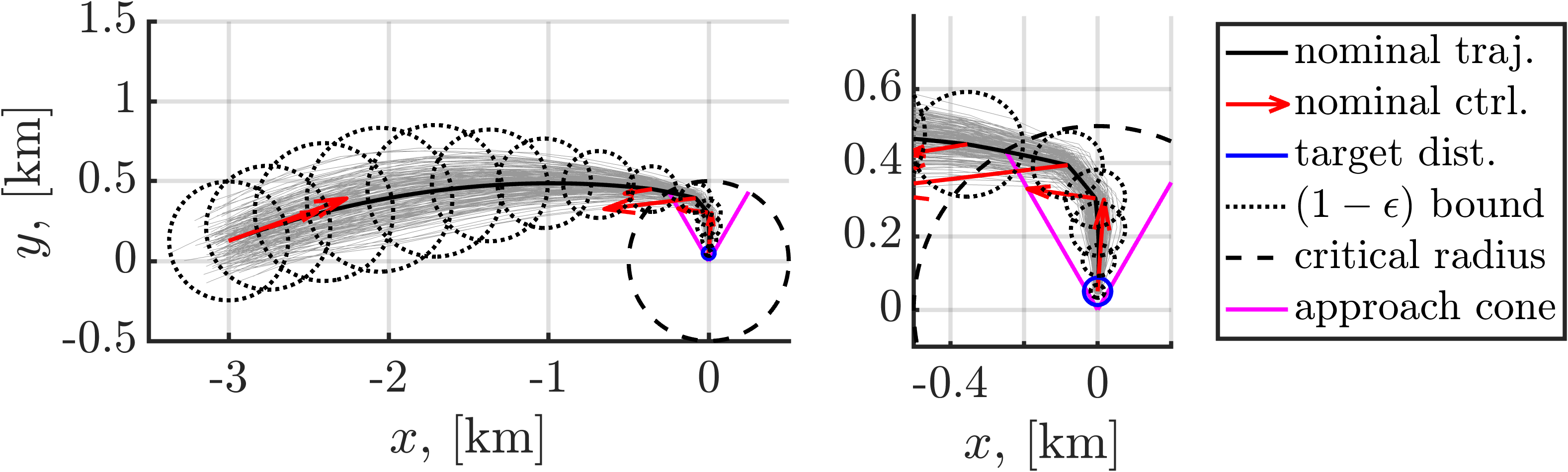
(a) Position 2-D projection: MC result with predicted statistics

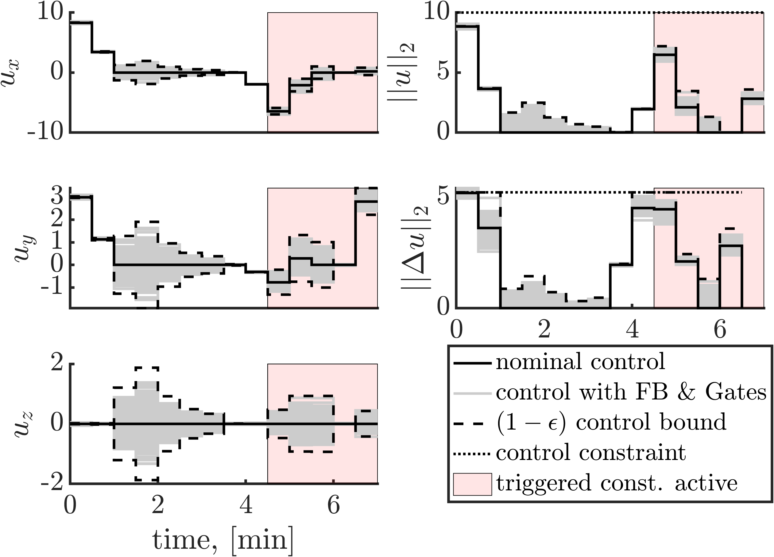
(b) MC results with predicted statistics, in (m/s)

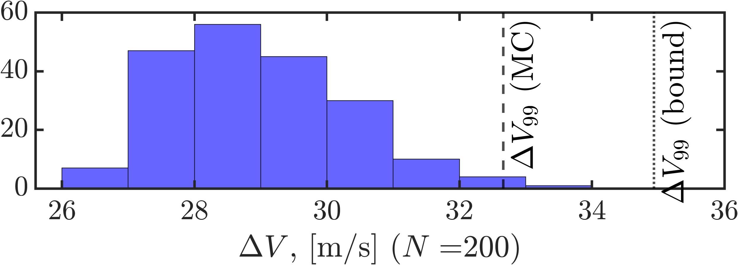
(c) MC total $\Delta V$ histogram & statistics

Figure 2: Safe autonomous rendezvous scenario with the approach cone constraint triggered when entering a sphere of critical radius $r_{\mathrm{trigger}}$.

As the problem involves a state-triggered constraint, Problem 3 is solved iteratively until the variable update is smaller than a tolerance $\epsilon_{\mathrm{tol}}{=}10^{-3}$. Each convex programming took $2.8{-}3.6$ seconds and the iteration was terminated by satisfying $\epsilon_{\mathrm{tol}}$ after 5 iterations. Monte Carlo (MC) simulation is performed using the designed control policies $\pi_{0:N-1}$.

Fig. 2 summarizes the MC result. Fig. 2(a) illustrates trajectories projected on the 2-D position space while Fig. 2(b) highlights $\bm{u}_{k}$, $\lVert\bm{u}_{k}\rVert_{2}$, and $\lVert\Delta\bm{u}_{k}\rVert_{2}$. These figures demonstrate that the designed policies $\pi_{1:N}$ successfully drive the state to the target distribution while satisfying all the chance constraints. Fig. 2(c) shows that $\Delta V_{99}$ from MC is indeed upper-bounded by $J_{\mathrm{ub}}$ with some optimality gap (${\sim}2$ m/s).

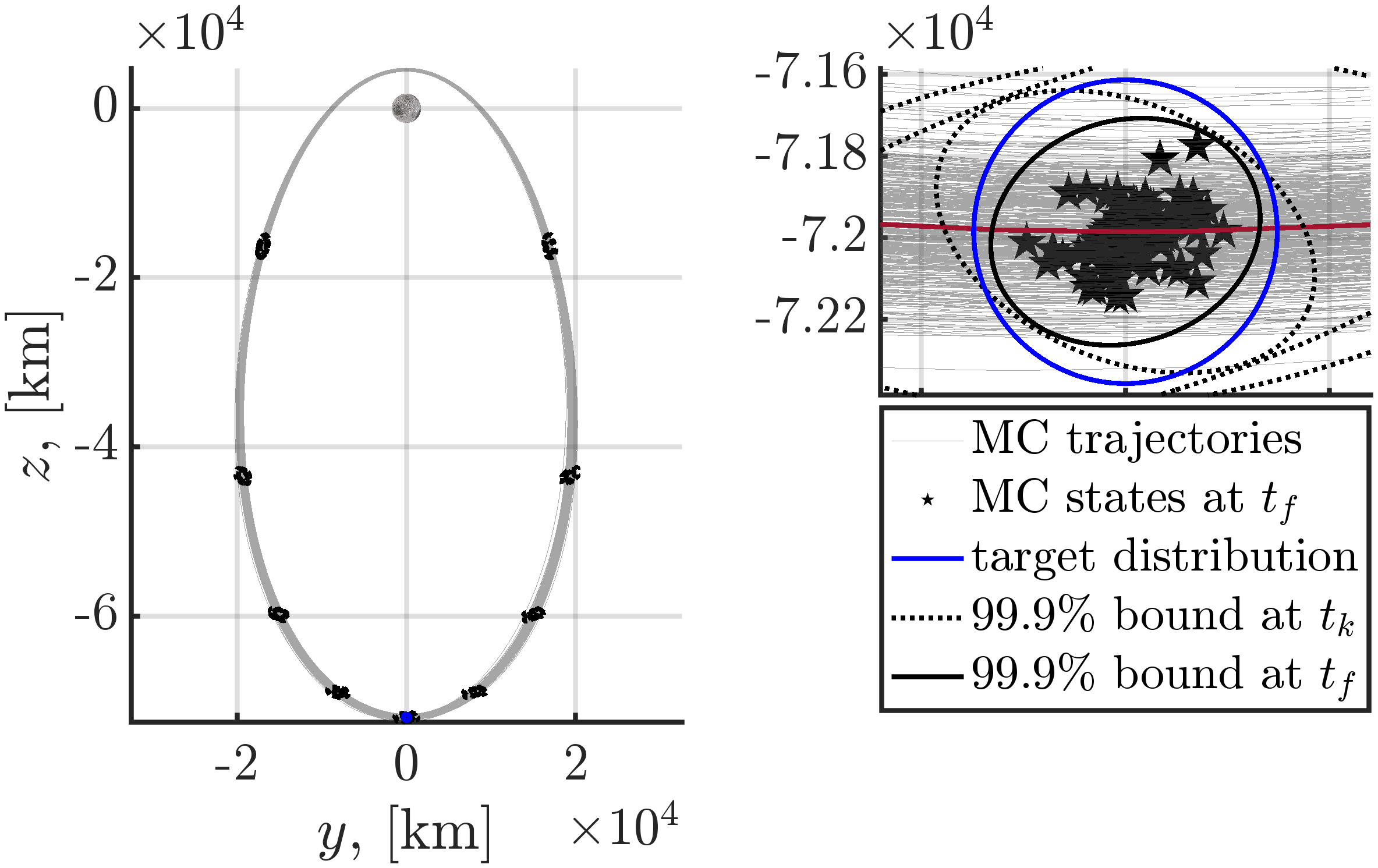
(a) Nonlinear MC trajectories & predicted statistics ($y$-$z$ projection)

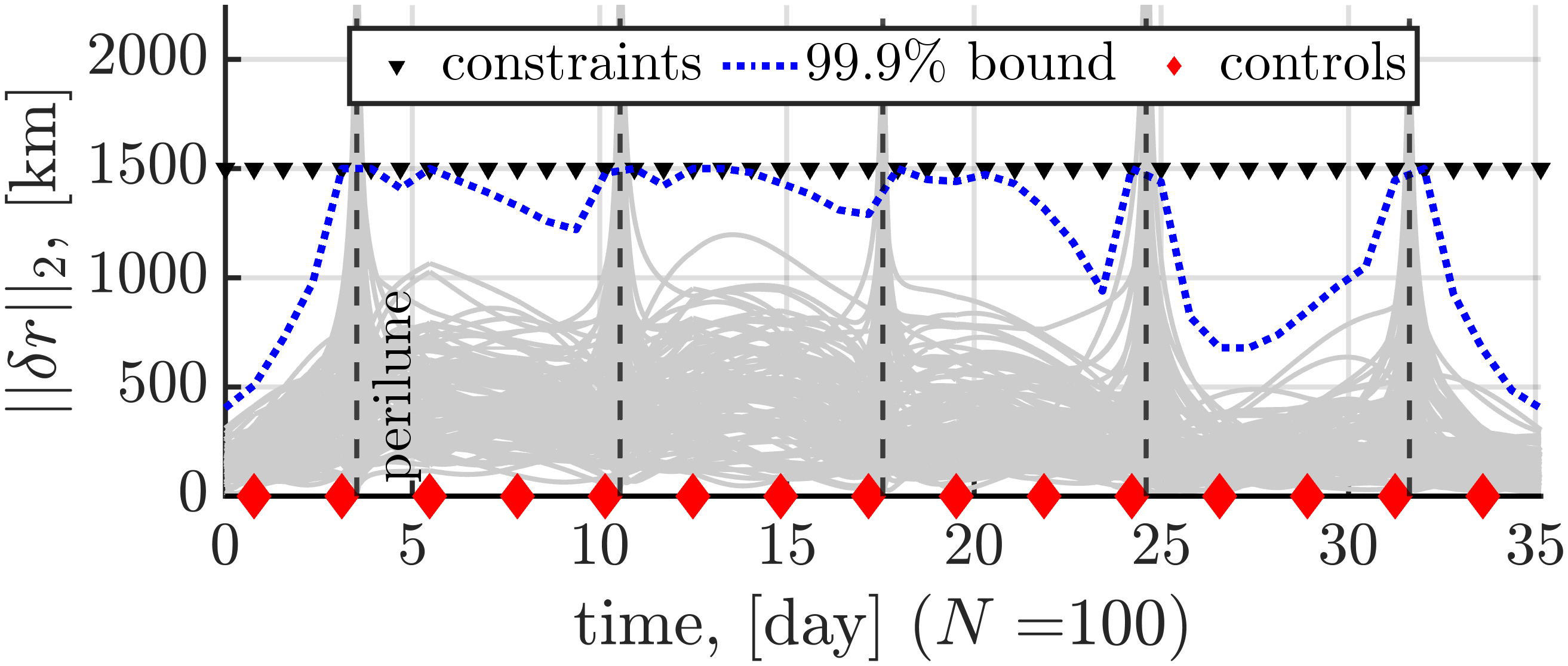
(b) MC position deviation; discrete-time c.c. successfully met

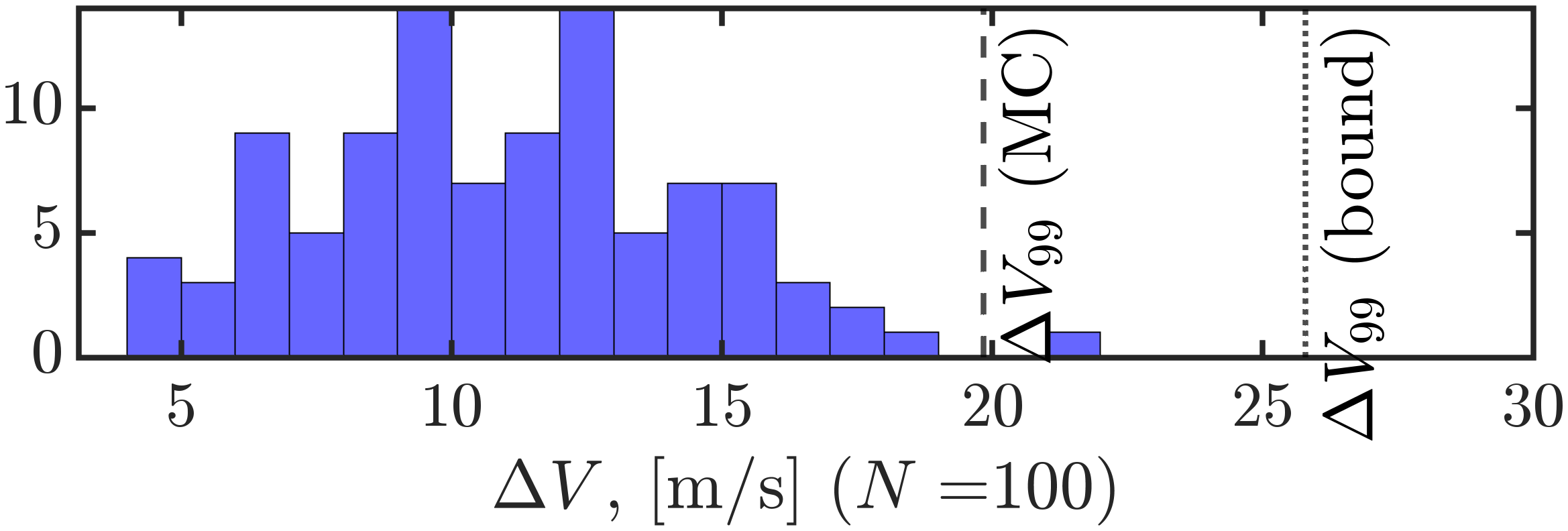
(c) MC total $\Delta V$ histogram & statistics

Figure 3: Safe autonomous cislunar L2 NRHO station-keeping scenario

V-B Safe NRHO Station-keeping Planning in Cislunar Space

Next consider safe station-keeping planning on a cislunar NRHO under uncertainty. For measurement modeling Eq. 11, we consider Moon horizon-based optical navigation (OpNav), which is originally proposed in [31] and applied to various cislunar orbits in [32]; we use the same OpNav parameters and filtering architecture as described in [32].

To apply the proposed framework, we linearize the nonlinear CR3BP EoM about a reference trajectory. We impose a tube-like constraint in Eq. 18 to constrain position deviations from the reference NRHO and control magnitude constraint in Eq. 19. The scenario begins at the apolune and considers 5 full NRHO revolutions, where $N=45$, i.e., 9 nodes are placed per orbit, evenly spaced in time, leading to $\Delta t\approx 0.8$ day. The spacecraft takes a measurement (moon image) at every node, and has trajectory correction maneuver (TCM) opportunities at every 3 nodes, that is, 3 TCM opportunities per orbit. Tube-like state chance constraints are imposed at every node. See Appendix for the parameters for NRHO, uncertainty modeling, and constraints.

Solving this problem does not require SCP as it does not have a state-triggered constraint, and is solved in ${\sim}8.4$ sec, producing about 35-day-worth safe control policy $\pi_{k}$.

Fig. 3 summarizes nonlinear MC results, verifying the robustness of $\pi_{k}$. The MC simulation nonlinearly evaluates $\bm{x}_{k}$, $\hat{\bm{x}}_{k}$, $\widetilde{\bm{y}}_{k}^{-}$, and $\bm{z}_{k}$: the nonlinear CR3BP EoM for $\bm{x}_{k}$ and OpNav-based extended Kalman filter (EKF) for $\hat{\bm{x}}_{k}$, $\widetilde{\bm{y}}_{k}^{-}$, and $\bm{z}_{k}$; EKF evaluates Eqs. 28, 29 and 30 along $\hat{\bm{x}}_{k}$ and $\hat{\bm{u}}_{k}$, and uses Eq. 13 instead of Eq. 31, which then affects $\bm{z}_{k}$ through Eq. 38. Fig. 3(a) shows the MC trajectories projected on $y$-$z$ plane and highlights the distributional constraint being met at $t_{f}$. Fig. 3(b) shows the satisfaction of the state chance constraints under the optimized policy. Fig. 3(c) indicates $\Delta V_{99}$ from MC is upper-bounded by $J_{\mathrm{ub}}$.

VI Conclusions

A safe spacecraft path-planning problem under uncertainty is formulated as an output-feedback, chance-constrained optimal control problem. The presented formulation exploits the Markovian property of the system and incorporates various chance constraints, including state-triggered chance constraints. The proposed planner designs a history of safe control policies by solving (sequential) convex programming, minimizing 99% quantile of control cost while ensuring the vehicle safety under uncertainties. The formulation is validated via safe autonomous rendezvous in proximity operations and safe cislunar NRHO station-keeping planning.

Appendix

Table I: CWH rendezvous scenario uncertainty parameters

Quantity	Symbol	Value	Unit
measurement error (pos.)	$\sigma_{\mathrm{obs},r}$	1.0	m
measurement error (vel.)	$\sigma_{\mathrm{obs},v}$	0.01	m/s
initial dispersion (pos.)	$\sigma_{r}$	100	m
initial dispersion (vel.)	$\sigma_{v}$	1.0	m/s
stochastic acceleration	$\sigma_{a}$	1.0	$\mathrm{mm/s^{3/2}}$
execution error (fixed mag.)	$\sigma_{1}$	1.0	cm/s
execution error (prop. mag.)	$\sigma_{2}$	1.0	%
execution error (fixed point.)	$\sigma_{3}$	1.0	cm/s
execution error (prop. point.)	$\sigma_{4}$	1.0	deg

Table II: CWH rendezvous scenario constraint parameters

Quantity	Symbol	Value	Unit
mean pos. at $t_{0}$	$\mskip 1.5mu\overline{\mskip-1.5mu{\bm{r}}\mskip-1.5mu}\mskip 1.5mu_{0}$	$[-3.0,\,0.126,\ 0]^{\top}$	km
mean vel. at $t_{0}$	$\mskip 1.5mu\overline{\mskip-1.5mu{\bm{v}}\mskip-1.5mu}\mskip 1.5mu_{0}$	$\bm{0}_{3\times 1}$	km/s
mean pos. at $t_{f}$	$\mskip 1.5mu\overline{\mskip-1.5mu{\bm{r}}\mskip-1.5mu}\mskip 1.5mu_{f}$	$[0.0,\,0.05,\ 0]^{\top}$	km
mean vel. at $t_{f}$	$\mskip 1.5mu\overline{\mskip-1.5mu{\bm{v}}\mskip-1.5mu}\mskip 1.5mu_{f}$	$\bm{0}_{3\times 1}$	km/s
pos. std. dev. at $t_{f}$	$\sigma_{r_{f}}$	10.0	m
vel. std. dev. at $t_{f}$	$\sigma_{v_{f}}$	0.1	m/s
max $\Delta V$ magnitude	$u_{\max}$	10.0	m/s
max attitude rate	$\omega_{\max}$	1.0	deg/s
approach cone angle	$\theta_{\max}$	30.0	deg
trigger critical radius	$r_{\mathrm{trigger}}$	0.5	km
rick bound (state)	$\epsilon_{x}$	$10^{-3}$	-
rick bound (control)	$\epsilon_{u}$	$10^{-3}$	-

VI-A Safe constrained rendezvous parameters

We consider $r_{0}=7228\leavevmode\nobreak\ \mathrm{km}$ for the chief’s orbit radius (${\sim}850$ km altitude). The time is discretized with interval $\Delta t=30\leavevmode\nobreak\ \mathrm{sec}$ with $N=14$.

We model the observation process as $\bm{f}_{\mathrm{obs}}(\bm{x}_{k})=\bm{x}_{k}$ and $G_{\mathrm{obs}}=\mathrm{blkdiag}(\sigma_{\mathrm{obs},r}I_{3},\sigma_{\mathrm{obs},v}I_{3})$, although the formulation can model more realistic measurements too (e.g., range, angle bearing). See Tables I and II for specific values.

Parameters that define other uncertainties are as follows. Initial state dispersion: $\hat{P}_{0}^{-}=\mathrm{blkdiag}(\sigma_{r}^{2}I_{3},\sigma_{v}^{2}I_{3})$. Initial estimate error: $\widetilde{P}_{0^{-}}=\mathrm{blkdiag}(\sigma_{\mathrm{obs},r}^{2}I_{3},\sigma_{\mathrm{obs},v}^{2}I_{3})$. Stochastic acceleration: $G=[0_{3\times 3},\sigma_{a}I_{3}]^{\top}$. The initial mean state and the target distribution are defined as: $\mskip 1.5mu\overline{\mskip-1.5mu{\bm{x}}\mskip-1.5mu}\mskip 1.5mu_{0}=[\mskip 1.5mu\overline{\mskip-1.5mu{\bm{r}}\mskip-1.5mu}\mskip 1.5mu_{0}^{\top},\mskip 1.5mu\overline{\mskip-1.5mu{\bm{v}}\mskip-1.5mu}\mskip 1.5mu_{0}^{\top}]^{\top}$, $\mskip 1.5mu\overline{\mskip-1.5mu{\bm{x}}\mskip-1.5mu}\mskip 1.5mu_{f}=[\mskip 1.5mu\overline{\mskip-1.5mu{\bm{r}}\mskip-1.5mu}\mskip 1.5mu_{f}^{\top},\mskip 1.5mu\overline{\mskip-1.5mu{\bm{v}}\mskip-1.5mu}\mskip 1.5mu_{f}^{\top}]^{\top}$, and $P_{f}=\mathrm{blkdiag}(\sigma_{r_{f}}^{2}I_{3},\sigma_{v_{f}}^{2}I_{3})$.

Parameters that define constraints are as follows. Maximum control rate: $\Delta u_{\max}=u_{\max}\omega_{\max}\Delta t$. Approach cone parameters: $A_{\mathrm{cone}}=\begin{bmatrix}1&0&0\\ 0&0&1\end{bmatrix}$ and $\bm{b}_{\mathrm{cone}}=[0,\tan{\theta_{\max}},0]^{\top}$, allowing the spacecraft to approach the chief from $+y$ direction with the cone angle $2\theta_{\max}$.

VI-B Safe NRHO station-keeping planning parameters

The observation process is modeled via Moon horizon-based oOpNav and uses the same parameters and filtering architecture as described in [32]. The parameters used for uncertainty modeling and constraints are listed in Tables III and IV. The NRHO initial condition is included in Table IV, where the state vector is in the non-dimensional unit, with the characteristic length and time in the Earth-Moon CR3BP being roughly $l_{*}=3.84748\times 10^{5}$ km and $t_{*}=3.75700\times 10^{5}$ sec. Note that the initial conditions must be obtained through a differential correction process [33] to design a tight multi-revolution NRHO for the use as a reference trajectory.

Table III: NRHO station-keeping scenario uncertainty parameters

Quantity	Symbol	Value	Unit
initial dispersion (pos.)	$\sigma_{r}$	100	km
initial dispersion (vel.)	$\sigma_{v}$	1.0	m/s
stochastic acceleration	$\sigma_{a}$	$10^{-4}$	$\mathrm{mm/s^{3/2}}$
execution error (fixed mag.)	$\sigma_{1}$	1.0	cm/s
execution error (prop. mag.)	$\sigma_{2}$	1.0	%
execution error (fixed point.)	$\sigma_{3}$	1.0	cm/s
execution error (prop. point.)	$\sigma_{4}$	1.0	deg

Table IV: NRHO station-keeping scenario constraint parameters

Quantity	Symbol	Value	Unit
mean pos. at $t_{0}$	$\mskip 1.5mu\overline{\mskip-1.5mu{\bm{r}}\mskip-1.5mu}\mskip 1.5mu_{0}$	$[1.0300,\,0.0,\ -0.1871]^{\top}$	nd
mean vel. at $t_{0}$	$\mskip 1.5mu\overline{\mskip-1.5mu{\bm{v}}\mskip-1.5mu}\mskip 1.5mu_{0}$	$[0.0,\,-0.1200,\ 0.0]^{\top}$	nd
mean pos. at $t_{f}$	$\mskip 1.5mu\overline{\mskip-1.5mu{\bm{r}}\mskip-1.5mu}\mskip 1.5mu_{f}$	$[1.0300,\,0.0,\ -0.1871]^{\top}$	nd
mean vel. at $t_{f}$	$\mskip 1.5mu\overline{\mskip-1.5mu{\bm{v}}\mskip-1.5mu}\mskip 1.5mu_{f}$	$[0.0,\,-0.1200,\ 0.0]^{\top}$	nd
pos. std. dev. at $t_{f}$	$\sigma_{r_{f}}$	100.0	km
vel. std. dev. at $t_{f}$	$\sigma_{v_{f}}$	1.0	m/s
max $\Delta V$ magnitude	$u_{\max}$	5.0	m/s
max state deviation	$d_{\max}$	1500	km
rick bound (state)	$\epsilon_{x}$	$10^{-3}$	-
rick bound (control)	$\epsilon_{u}$	$10^{-3}$	-

References

• [1] J. A. Starek, B. Açıkmeşe, I. A. Nesnas, and M. Pavone, “Spacecraft Autonomy Challenges for Next-Generation Space Missions,” in Advances in Control System Technology for Aerospace Applications (E. Feron, ed.), Lecture Notes in Control and Information Sciences, pp. 1–48, Berlin, Heidelberg: Springer, 2016.
• [2] M. Ono, B. C. Williams, and L. Blackmore, “Probabilistic planning for continuous dynamic systems under bounded risk,” Journal of Artificial Intelligence Research, vol. 46, pp. 511–577, 2013.
• [3] K. Okamoto, M. Goldshtein, and P. Tsiotras, “Optimal Covariance Control for Stochastic Systems Under Chance Constraints,” IEEE Control Systems Letters, vol. 2, pp. 266–271, Apr. 2018.
• [4] J. Ridderhof, K. Okamoto, and P. Tsiotras, “Chance Constrained Covariance Control for Linear Stochastic Systems With Output Feedback,” in 2020 59th IEEE Conference on Decision and Control (CDC), vol. 2020-Decem, pp. 1758–1763, IEEE, Dec. 2020.
• [5] G. Gaias and S. D’Amico, “Impulsive Maneuvers for Formation Reconfiguration Using Relative Orbital Elements,” Journal of Guidance, Control, and Dynamics, vol. 38, no. 6, pp. 1036–1049, 2015.
• [6] B. Açıkmeşe and S. R. Ploen, “Convex Programming Approach to Powered Descent Guidance for Mars Landing,” Journal of Guidance Control and Dynamics, vol. 30, no. 5, pp. 1353–1366, 2007.
• [7] P. Lu and X. Liu, “Autonomous Trajectory Planning for Rendezvous and Proximity Operations by Conic Optimization,” Journal of Guidance, Control, and Dynamics, vol. 36, pp. 375–389, Mar. 2013.
• [8] T. Ito and S. Sakai, “Throttled explicit guidance for pinpoint landing under bounded thrust acceleration,” Acta Astronautica, vol. 176, pp. 438–454, Nov. 2020.
• [9] P. Lu, “Predictor-Corrector Entry Guidance for Low-Lifting Vehicles,” Journal of Guidance, Control, and Dynamics, vol. 31, no. 4, pp. 1067–1075, 2008.
• [10] R. Furfaro, D. Cersosimo, and D. R. Wibben, “Asteroid precision landing via multiple sliding surfaces guidance techniques,” Journal of Guidance, Control, and Dynamics, vol. 36, no. 4, pp. 1075–1092, 2013.
• [11] A. Weiss, M. Baldwin, R. S. Erwin, and I. Kolmanovsky, “Model Predictive Control for Spacecraft Rendezvous and Docking: Strategies for Handling Constraints and Case Studies,” IEEE Transactions on Control Systems Technology, vol. 23, pp. 1638–1647, July 2015.
• [12] S. Di Cairano, H. Park, and I. Kolmanovsky, “Model Predictive Control approach for guidance of spacecraft rendezvous and proximity maneuvering,” International Journal of Robust and Nonlinear Control, vol. 22, no. 12, pp. 1398–1427, 2012.
• [13] M. V. Kothare, V. Balakrishnan, and M. Morari, “Robust constrained model predictive control using linear matrix inequalities,” Automatica, vol. 32, no. 10, pp. 1361–1379, 1996.
• [14] Y. Kuwata, A. Richards, and J. How, “Robust receding horizon control using generalized constraint tightening,” in American Control Conference, (New York, NY), pp. 4482–4487, Institute of Electrical and Electronics Engineers (IEEE), July 2007.
• [15] C. Buckner and R. Lampariello, “Tube-Based Model Predictive Control for the Approach Maneuver of a Spacecraft to a Free-Tumbling Target Satellite,” in 2018 Annual American Control Conference (ACC), pp. 5690–5697, June 2018.
• [16] C. E. Oestreich, R. Linares, and R. Gondhalekar, “Tube-Based Model Predictive Control with Uncertainty Identification for Autonomous Spacecraft Maneuvers,” Journal of Guidance, Control, and Dynamics, vol. 46, no. 1, pp. 6–20, 2023.
• [17] R. H. Battin, An Introduction to the Mathematics and Methods of Astrodynamics, Revised Edition. 1999.
• [18] K. T. Alfriend, S. R. Vadali, P. Gurfil, J. P. How, and L. S. Breger, Spacecraft Formation Flying: Dynamics, Control and Navigation. 2010.
• [19] V. Szebehely, Theory of Orbit: The Restricted Problem of Three Bodies. Academic Press Inc., 1967.
• [20] C. R. Gates, “A simplified model of midcourse maneuver execution errors,” tech. rep., Jet Propulsion Laboratory, California Institute of Technology (Report No. 32-504), Pasadena, CA, Oct. 1963.
• [21] K. Oguri and J. W. McMahon, “Robust Spacecraft Guidance Around Small Bodies Under Uncertainty: Stochastic Optimal Control Approach,” Journal of Guidance, Control, and Dynamics, vol. 44, pp. 1295–1313, July 2021.
• [22] N. Kumagai and K. Oguri, “Robust NRHO Station-keeping Planning with Maneuver Location Optimization under Operational Uncertainties,” in AAS/AIAA Astrodynamics Specialist Conference, (Big Sky, MT), 2023.
• [23] K. Oguri, M. Ono, and J. W. McMahon, “Convex Optimization over Sequential Linear Feedback Policies with Continuous-time Chance Constraints,” in IEEE 58th Conference on Decision and Control (CDC), pp. 6325–6331, Dec. 2019.
• [24] M. Szmuk, T. P. Reynolds, and B. Açıkmeşe, “Successive Convexification for Real-Time Six-Degree-of-Freedom Powered Descent Guidance with State-Triggered Constraints,” Journal of Guidance, Control, and Dynamics, vol. 43, pp. 1399–1413, Aug. 2020.
• [25] D. Aleti, K. Oguri, and N. Kumagai, “Chance-Constrained Output-Feedback Control without History Feedback: Application to NRHO Stationkeeping,” in AAS/AIAA Astrodynamics Specialist Conference, (Big Sky, MT), 2023.
• [26] A. Nemirovski and A. Shapiro, “Convex Approximations of Chance Constrained Programs,” SIAM Journal on Optimization, vol. 17, no. 4, pp. 969–996, 2006.
• [27] K. Oguri and G. Lantoine, “Stochastic Sequential Convex Programming for Robust Low-thrust Trajectory Design under Uncertainty,” in AAS/AIAA Astrodynamics Specialist Conference, 2022.
• [28] J. Ridderhof, J. Pilipovsky, and P. Tsiotras, “Chance-constrained Covariance Control for Low-Thrust Minimum-Fuel Trajectory Optimization,” in AAS/AIAA Astrodynamics Specialist Conference, (South Lake Tahoe, CA (Virtual)), AAS, Aug. 2020.
• [29] Y. Mao, M. Szmuk, and B. Acikmese, “Successive convexification of non-convex optimal control problems and its convergence properties,” in IEEE 55th Conference on Decision and Control (CDC), pp. 3636–3641, IEEE, Dec. 2016.
• [30] K. Oguri, “Successive Convexification with Feasibility Guarantee via Augmented Lagrangian for Non-Convex Optimal Control Problems,” in 2023 62nd IEEE Conference on Decision and Control (CDC), (Singapore, Singapore), pp. 3296–3302, IEEE, Dec. 2023.
• [31] J. A. Christian and S. B. Robinson, “Noniterative Horizon-Based Optical Navigation by Cholesky Factorization,” Journal of Guidance, Control, and Dynamics, vol. 39, pp. 2757–2765, Dec. 2016.
• [32] D. C. Qi and K. Oguri, “Analysis of Autonomous Orbit Determination in Various Near-Moon Periodic Orbits,” The Journal of the Astronautical Sciences, 2023.
• [33] T. A. Pavlak, Trajectory Design and Orbit Maintenance Strategies in Multi-Body Dynamical Regimes. PhD thesis, Purdue University, 2013.