A contact map method to capture the features of knot conformations
Abstract
Inspired by recent advances in the chromosome capture techniques, a method is proposed to study the structural organization of systems of polymers rings with topological constraints. To this purpose, the system is divided into compartments and a simple condition is provided in order to determine if two compartments are in contact or not. Next, a set of contact matrices is defined that count how many times during a simulation a compartment was found in contact with a non-contiguous compartment in conformations with a given energy or temperature. Similar strategies based on correlation maps have been applied to the study of knotted polymers in the recent past. The advantage of the present approach is that is coupled with the Wang-Landau algorithm. Once the density of states is computed, it is possible to generate the contact matrices at any temperature. This gives an immediate overview over the changes of phases that polymer systems undergo. The information on the structure of knotted polymers and links stored in the contact matrices is the result of averaging hundred of billions of conformations and visualized by means of colormaps. The obtained color patterns allow to identify the main properties of the structure of the system under investigation at any temperature. The method is applied to detect the structural rearrangements following the phase transitions of a knotted polymer ring and a circular polycatenane composed by four rings in a solution. It is shown that the colormaps have a finite number of patterns that can be clearly associated with the different phases of these systems. The results agree with the available data coming from the plots of the observables and the close inspection of snapshots of the system taken at different steps of the simulations. They also bring new knowledge, for instance predicting the average number of tails appearing in the conformations of the considered polymers at a given temperature.
I Introduction
In this work a method is presented to measure the frequency of the interactions between the segments of a system consisting of one or more polymers. The method is inspired by the recent advances in the techniques that capture the conformations of the chromosomes like the Hi-C technique Hi-C . Each polymer of the system is divided into compartments containing a number of monomers. A simple criterion to decide if two compartments and are getting close is provided: Namely, the distance between their centers of mass should be smaller than the sum of their radii of gyration. A set of contact matrices is defined, whose elements count the total number of times in which any pair of compartments of a conformation of energy has satisfied this criterion during a simulation of the analyzed polymer system. In our setup, the polymers are coarse grained and defined on a simple cubic lattice. The random sampling of their conformations is performed in the microcanonical ensemble using the Wang-Landau Monte Carlo algorithm wl that allows to compute the density of states for any value of the energy . It turns out that the contact matrices are an useful tool in order to understand the structural organization of a polymer system at the given energy . By passing from the microcanonical ensemble to the canonical ensemble, it is also possible to study the structural rearrangements following a phase transition. The method presented in this work is able to capture the main features of states of given energy or temperature after averaging over hundred of billions of sampled conformations. To analyze such a wealth of data using more traditional tools could slow down considerably the simulations. Here it is just sufficient to look at the darker or brighter tones of the colormaps generated from the contact matrices. Brighter or darker tones occur depending on the frequency with which two compartments were found to be close during a given simulation.
The validity of our approach has been checked by applying it to knotted polymers edwards ; degennes and circular polycatenanes LTFFEO2022 ; liu in a solution. We present here two study-cases: a knotted polymer with the topology of a knot and a circular catenane. The phase transitions of these systems are detected by looking at the plots of their specific heat capacity with respect to the temperature. The main changes of the structures characterizing the different phases of the considered polymers are determined using the colormaps obtained from the contact matrices computed at temperatures that are lower or higher than the temperature at which a given phase transition is occurring. Conformations stored randomly during the simulations are inspected in order to verify that the properties predicted from the colormap are frequently occurring as it is expected.
Concluding, we would like to mention some of the previous studies that use other approaches but are relevant for this work. The statistical mechanics of open or circular copolymers has been extensively investigated in the past, see e. g. marko ; vilgis ; holystvilgis ; huber ; metzler ; binder ; kudaibergenov . Systems similar to those treated here have been considered in velyaminov ; kardar and, more recently, in mella ; mella2 . There has been also some interest on circular diblock copolymers with non-trivial topologies orlandinibaiesizontaworkonstiffness ; daietal ; vlahosetal ; najafi ; kuriatasikorski ; benahmed ; mella ; kumar . Some more general systems have been considered in relation to specific aspects, like for instance the knotted Hydrophilic-Polar (HP) models in proteins dill ; wuest ; wuest2 , knotted proteins on the lattice achille ; patricia and the self-assembly of nanomaterials of specific topologies controlled by tuning the properties of patchy heteropolymers ivan . Previous studies of the statistical mechanics of knotted homopolymers and copolymers with the help of the Wang-Landau algorithm wl can be found for example in velyaminovhomopolymers ; swetnam (homopolymers) and wang ; NATFFMPLT2023 (copolymers). There exist also sophysticated alternative methods to investigate the structure of knots. For example, Kymoknot kymoknot is a C code to identify and localize knots based on the Alexander polynomial and Topoly is a Python package to characterize the topology of proteins topoly . The HOMFLYPT, Kauffman, and Jones polynomials are implemented in Knotplot knotplot , Topoly, in the Mathematica KnotData package, and in Python Sage sage . An approach similar in spirit to that discussed here has been recently applied to the study of the dynamics of prime knots lappala . The algorithm that has been used in that work to generate the contact matrices is based on the correlations between the root-mean-squared fluctuations of individual particles of a knot. In our approach not individual particles, but compartments are considered. The size of the compartments allows to change the resolution under which the knotted polymers or links are investigated. Another difference is that the present method has been combined with the Wang-Landau algorithm and is specialized to the study of the phase transitions. More in general, it is able to detect the properties of polymer systems in presence of topological constraints at any temperature.
The material presented in this work has been divided as follows. Section II is an introduction to the used methodology. In particular, in Subsection II.1 the main features of the Wang-Landau Monte Carlo algorithm are explained, while Subsection II.2 is dedicated to the construction of the contact matrix and to the visualization of the data stored in it using colormaps. The proposed method is then applied in Section III in order to understand the structural rearrangements following the phase transitions of a single knotted polymer (Subsection III.1) and a polycatenane composed by four concatenated rings (Subsection III.2).
II Methodology
II.1 The Wang-Landau method used
The method presented in this work has been tested using as a model polymer rings in a solution. The monomers are located on the sites of a simple cubic lattice and each lattice site can be occupied by at most one monomer. Two consecutive monomers on the loop are linked by one lattice bond, so that the total length of the knot in lattice units is equal to . The polymers considered here are diblock copolymers with monomers of type and monomers of type . Of course, . The short-range interactions between the monomers are described by following Hamiltonian:
| (1) |
In Eq. (1) is an arbitrary conformation of the system. For a given conformation , the quantities ’s, where , count the number of couples composed by a monomer of type and a monomer of type satisfying the following relations:
| (2) |
Here denote the locations of the monomers and the indices and take all values from to . The first condition of Eq. (2) is due to the fact that two contiguous monomers along the backbone of the polymer are not interacting. is an energy scale measuring the cost for two non-contiguous monomers and to be found at the minimal allowed distance: . can be positive or negative. Finally, the are coefficients that can take only three values: and . Two monomers and of types and respectively are said to form a bond whenever and the two conditions (2) are satisfied. They s are used together with to determine the setup. For instance, by putting , we obtain a system of charged monomers, with the monomers of type having opposite charge with respect to monomers of type . In this case, the Hamiltonian (1) describes the case discussed in NATFFMPLT2023 . of Coulomb interactions screened by the presence of ions in the solution. Alternatively, choosing , and , the knotted polymer becomes an homopolymer in a good solvent for and in a bad solvent for . The used setups are summarized in Table 1. In that table, the case diblock copolymers I refers to the charged monomers mentioned before. In diblock copolymers II the solvent is good for the monomers of type and bad for those of type .
| setup | ||||||
|---|---|---|---|---|---|---|
| homopolymers | ||||||
| in good solvent | ||||||
| homopolymers | ||||||
| in a bad solvent | ||||||
| diblock | ||||||
| copolymers I | ||||||
| diblock | ||||||
| copolymers II |
For convenience, thermodynamic units will be chosen in which the Boltzmann constant is equal to one. In these units the temperature is related to the usual temperature by the relation: . We will also introduce the rescaled temperature . Clearly, the ratio , where :
| (3) |
More details are given in Ref. NATFFMPLT2023 .
The simulations are performed using the Wang-Landau Monte Carlo algorithm wl . The initial knot conformations are obtained by elongating the existing conformations of minimal length knots rechnitzer ; sharein until the desired final length is attained. The details on the sampling and the treatment of the topological constraints can be found in Refs. yzff and yzff2013 . The random transformations that are necessary for sampling the different knot conformations are the pivot moves of Ref. madrasetal . In order to preserve the topological state of the system, the pivot algorithm and excluded area (PAEA) method of Ref. yzff is applied.
The partition function of the polymer knot is given by:
| (4) |
where denotes the density of states:
| (5) |
is the quantity to be evaluated via Monte Carlo methods. The expectation values of any observable may be computed using the formula:
| (6) |
Here denotes the average of over all sampled states with rescaled energy .
II.2 The contact matrix
To construct the contact matrix, the polymer under investigation is divided into ”compartments” with monomers each. Supposing that the polymer has a total of monomers, the number of compartments is .
Let’s label these compartments with the first letters of the Latin alphabet . During the sampling, every time a compartment gets ”in contact” with another compartment , the element of the contact matrix is updated as follows:
| (7) |
where is some small real number, for instance . Of course:
| (8) |
The condition for which two compartments are considered in contact will be provided in the following. First, the gyration radii and of the two compartments is computed. The two compartments and are said to be in contact if the distance between their centers of mass satisfies the relation:
| (9) |
The above procedure produces the contact matrix that counts how many times during a simulation a conformation is found such that two compartments and are in contact for . The data stored in may be visualized using a colormap. For instance, in the colormap darker colors can be assigned to pairs of compartments that have resulted to be more frequently distant from each other and lighter colors to pairs that were closer. This convention will be used in all the colormaps presented here.
At least in principle, these data deliver an information about the shape of knotted polymers. However, in a typical simulation hundred of billions of random conformations are generated. These conformations have very different shapes, from extremely compact to extremely expanded and any case inbetween. It is difficult to capture the average features of such a wealth of conformations. To obtain meaningful results, a further refinement is necessary consisting in the introduction of a new contact matrix . is defined exactly like the full matrix , but with the restriction that only conformations with a fixed energy are considered. Even with this restriction, the variety of shapes is still enormous. Yet, the performed simulations show that the matrix is able to capture the common features characterizing the conformations of given energy despite the fact that the shapes of these conformations strongly differ from each other. Indeed, we have observed that after a sufficient number of samples has been generated, the colormap stabilizes and there are no more significant changes of the patterns formed by the darker and lighter areas of the map. Of course, during the sampling the elements are steadily growing because of the addition of the small quantity in Eq. (7), However, denoting by and the contact matrices computed after taking into account and conformations respectively, we have that:
| (10) |
where and is a scaling factor independent of and . In other words, when large amounts of conformations have been explored, the ratio
| (11) |
converges to a given value which does not change if further samples are considered. While convergence require , this is not a problem because, during a simulation, a very high number of conformations is explored, usually of the order or higher. The conditions (10) and (11) have been verified in all performed simulations.
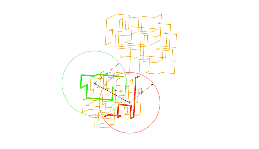
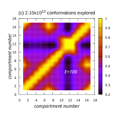
We would also like to stress that the information stored in the matrices is robust with respect to changes in the choice of , i. e. the parameter that determines the resolution under which a knotted polymer is observed. More precisely, supposing that , a colormap generated from a matrix computed using the lower resolution , but interpolated over a larger number of points, presents the same patterns of bright and dark areas as the colormap obtained with the higher resolution , see Fig. 2. Of course, in the limiting case , in which the compartment coincides with the whole system, the resolution will be too low to get some useful information about the polymer conformations from the matrix . On the other hand, too small compartments, let’s say with , have a too small radius, so that Eq. (9) can hardly be applied.
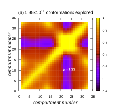
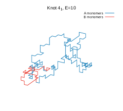
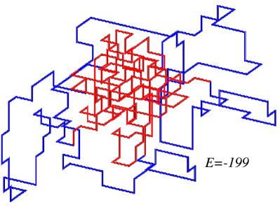
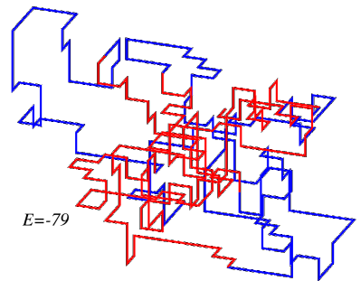
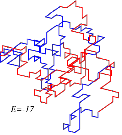
As an example to illustrate the above settings, in Fig. 2 a few colormaps are shown corresponding to the knotted homopolymer of Fig. 1. The topology of the system is that of a composite knot . The total number of monomers is . The resolution has been set by putting , so that there are compartments. To take into account the fact that the polymer forms a closed curve in space, a fictitious compartment has been added whose entries in the contact matrix coincide with those of the first compartment. Accordingly, the colormaps are divided into small sectors corresponding to the elements of . Moreover, the small sectors on the opposite edges of the colormaps are identified as in the rectangle representing a torus on a two dimensional plane. Finally, in the reduced Hamiltonian of Eq. (3) describing the energy of the system the parameters have been chosen according to the setup homopolymer in a good solvent, see Table 1. More information can be found in the captions of Fig. 1. We would like to stress the presence of cross-links constraining the knots and to be confined within the compartments and respectively.
The data used in panels (a) and (b) come from the matrices taken after considering and conformations respectively. The energy is the average energy of the system at the temperature . In panel (c) the resolution has been reduced to , but a higher interpolation level has been applied. As it is possible to see, the color patterns in panel (a) and (b) are practically the same and they are in a good agreement with that of panel (c). Let us notice that the range of values corresponding to the colors in panel (a) (from 0.4 to 1) is different from that of panel (b), which goes from 0.55 up to 1. However, the elements of the matrix in panel (a) that are within the interval consist of less than 7% of the total of elements. This is why their presence does not introduce substantial changes in the colormap of panel a) with respect to that of panel (b). Small discrepancies like this may occur even at very high values of because, while the system is ergodic, certain conformations need a considerable amount of time before being generated started from a given seed.
In the next Section we will use the following notation to identify an arbitrary sector on a colormap: . For instance, the sector coincides with the strip in panel (a) of Fig. 2 in which the purple color is dominant. This means that the compartments have a low chance to get in contact with the compartments .

III Application of the technique: capturing the structure of knotted polymers
The contact matrix method presented in the previous Section is a helpful tool in understanding the structure of knotted polymers and the structural reorganizations that they undergo during phase transitions. It is particularly useful within the Wang-Landau method, because in that case the sampling is performed in the microcanonical ensemble, where the temperature is not known. This makes it difficult to take snapshots of the conformations that could show the structure of knotted polymers below and above the transition temperature. Once the matrices defined in the previous Section are computed for all values of the energy , the matrices in the temperature domain can be recovered using Eq. (6):
| (12) |
counts how frequently two compartments and have been found in contact at a given temperature during a simulation.
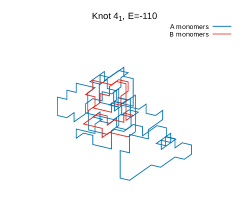
III.1 Case of a knotted polymer with topology and
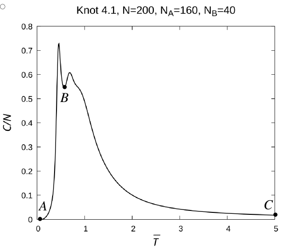
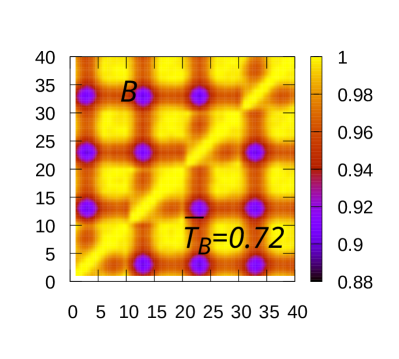
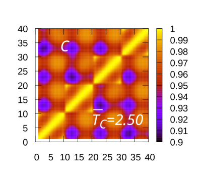
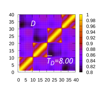
To show how an information about the structural organization of knotted polymers can be retrieved, we consider as a first example a ring with monomers and the topology of a knot. Let the setup be that of diblock copolymers I of Table 1 with and . The number of monomers in a compartment is , so that each conformation is divided into compartments. The first compartments contain monomers of type , while the last eight contain monomers of type . This system, characterized by an excess of monomers, is known to exhibit three distinct phases as explained in NATFFMPLT2023 : a mixed phase (phase) at the lowest temperatures, an intermediated phase (phase) and an unmixed phase (phase) at high temperatures. The mixing is between the and monomers. The plot of the specific heat capacity of this system shows two peaks, see Fig. 3. They correspond to the transitions and . In the figure the points and correspond to the temperatures and respectively. At the phase dominates, while at and the systems is in the and phases respectively.
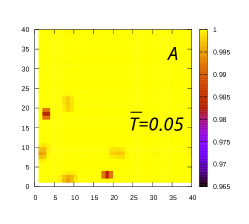
In Fig. 4 the colormaps obtained from the matrices are shown. As it is possible to see, in all of them the central diagonal is yellow, which is the color corresponding to the highest possible value in all colorbars. This is expected, because it is very likely that two contiguous compartments are getting in contact. Another common feature is that the values in the colorbars are ranging within small intervals, the largest of them being [0.955,1.000] in the right panel of Fig.4. This is explained by the fact that the colormaps are the result of the averaging over hundred of billions of conformations. As a consequence, no matter how two compartments and are located along the polymer backbone, it is well possible that there is a statistically relevant set of conformations in which and are close. For this reason, the differences between the elements can be small. However, as we will see these differences produce colormaps that are able to distinguish the various phases of knotted polymers . The range of the colorbar is of course sensitive to the presence of constraints. For instance, the interval of values in the colorbars of Fig. 2 is large because of the crosslinks that limit the movements of the compartments of the composite knot discussed in Section II. An extended range is likely to occur also when the set of conformations belonging to a given phase is small. In this case, the limited number of available conformations could be characterized by a restricted number of shapes preventing some of the compartments to get close to each other.
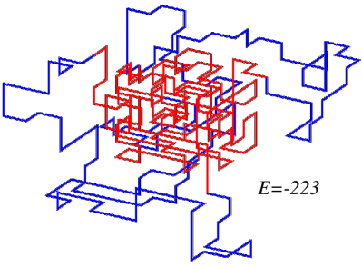
Coming back to Fig. 4, we note that the colormaps exhibit three quite distinct patterns. These patterns correspond to the structural organizations of the system in the three available phases. In fact, they remain stable if the temperature is increased or decreased and change only when one of the two peaks of the specific heat capacity is crossed. Similar colormaps as that in the left panel of Fig. 4 are observed at the lowest temperatures in which . The figure shows the colormap in the particular case . The distribution of darker and brighter colros is compatible with the conformations of the phase described in Ref. NATFFMPLT2023 . An example of such conformations, corresponding to the lowest possible energy , is provided in Fig. 5, left panel. In this phase there is a high level of mixing between the and monomers. The reason is that, in the chosen setup of diblock copolymers I, the and monomers are subjected to attractive forces. As a consequence, approximately in the range of temperatures , the monomers belonging to different types form bonds in order to minimize the energy of the knotted polymer. The result is that the conformations are very compact and the monomers are closely packed together. This is visible in the colormap of Fig. 4, left panel, where yellow is everywhere the dominant color. Of course, due to the excess of monomers, which repel themselves, not all the monomers are able to bind with the limited number of monomers available. As a result, small tails of monomers departing from the bulk are appearing, see Fig. 5, left panel. We associate these tails with the darker spots appearing in the colormap of Fig. 4, left panel. From the colormap it turns out that the comparments and are responsible for the largest tail, as they are the most likely to be distant from each other. Indeed, the sector is the darkest one.
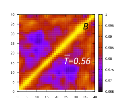

At higher temperatures, in the interval between the two peaks of the heat capacity of Fig. 3 around , knotted polymers with are in the phase NATFFMPLT2023 . The colormap in Fig. 4, central panel, corresponds to the structural organization of the conformations typical of this phase. The sector is predominantly yellow-red as a consequence of the fact that the monomers in compartments are forming bonds with the monomers in compartments . The result is a compact bulk held together by these bonds that is similar, but smaller than that of the phase. The level of mixing between the and monomers is high. The substantial difference from the previous phase is the large violet area showing that the monomers in different compartments have a lower chance to get close to each other. This is compatible with the presence in the phase of longer tails departing from the compact bulk. These tails are the effect of the increased thermal fluctuations that counteract the attractive interactions between the and monomers. As a consequence, the latter are no longer able to sustain a large bulk as in the phase and consistent portions of the segment containing the monomers are floating outside a smaller bulk. The polymer conformation in Fig. 5, central panel, of energy is indeed characterized by a compact bulk with long tails.
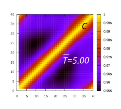
As the temperature increases further, the interactions between the monomers are overwhelmed by the strong thermal fluctuations. As it is possible to see in Fig. 4, right panel, the lighter yellow area is concentrated in the diagonal of colormap , implying that mainly the contiguous compartments are able to get close to each other. The remaining area of the colormap is predominantly black or violet. The fact that the violet color is concentrated in the sector has a simple explanation: It means that at the very high temperature there is still some residual effect of the attractive interactions between the monomers in compartments and the monomers in compartments .
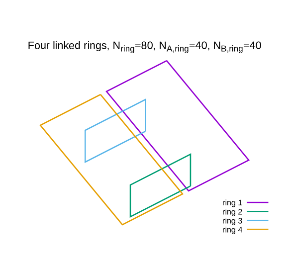
III.2 Case of a circular catenane
In this subsection, the contact matrices will be applied to study the structural organizations at different temperatures of the circular catenane shown in Fig. 6. This system is composed by four polymer rings concatenated together of length each. The setup of each ring is that of diblock copolymers II, see Table 1, with monomers of the type and monomers of the type. The total number of monomers in the system is . Each compartment contains monomers. Accordingly, there are compartments in the circular catenane and the Hi-C matrix has dimension . Since each ring composing the link contains 10 compartments, it is convenient to divide the Hi-C colormap into 16 sectors , , of dimension . For instance, denotes the sector x(21:30),y(31:40). The sectors may be considered as smaller colormaps providing information about the average locations of the compartments of the th ring with respect to the compartments of the th ring. The diagonal sectors , capture the structural organization of the single rings. It will also be convenient to distinguish inside a sector the four subsectors , , and . For example, represents the colormap of dimension which tells how distant are in the average the five compartments of ring containing monomers from the five compartments containing monomers of ring .
The specific heat capacity of the circular catenane is characterized by two peaks and a shoulder at , see Fig. 7.
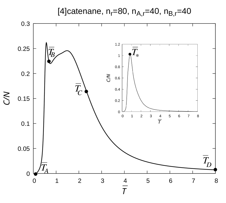
Following rampf ; janke ; janke2 ; hsieh ; privalov , peaks and shoulders appear in connections with phase transitions. This implies that the system admits four distinct phases and three phase transitions. The most important features of the structural organization of the circular catenane in all these four phases can be determined with the help of the Hi-C colormaps. It turns our that there are two levels of organization: that of the single rings and that of the circular catenane as a whole.
The first phase appears at the lowest temperatures. In the colormap taken at in Fig. 8, left panel, yellow is the dominant color. Since yellow corresponds in the colorbar to the highest probability that two compartments are found close to each other, it is possible to conclude that the rings composing the circular catenane as well as the whole system are in compact conformations.
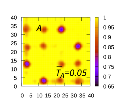
As already mentioned, the information about the th ring is stored in the sector , which is mainly colored with bright yellow. This means that the rings are in a collapsed phase. This could be expected in the case of the compartments containing the monomers because in the chosen setup diblock copolymer II they are subjected to attractive interactions. More surprisingly is that also the compartments with the monomers, which repel themselves, can be found near to each other as it is easy to realize by looking at the subsectors , of the colormap of Fig. 8, left panel. All these subsectors are indeed colored with yellow. This is however not a contradiction, because only the formation of bonds can change the energy according to the Hamiltonian (1). The condition (9) for two compartments to become close does not necessarily imply that the monomers of these compartments are forming bonds. Concerning the global structure of the circular catenane, we notice that yellow is the dominant color in the sectors outside the diagonal, i. e. with . The fact that the subsectors with are yellow suggest that the compartments with the monomers are densely packed together due to the attractive interactions and form a compact bulk within the circular catenane. Instead, the subsectors with are much darker than all the other subsectors. To fix the ideas, let’s consider in the colormap of Fig. 8, left panel, the three dark spots that are visible in the sector x(1:5),y(1:40). The presence of the first spot in the subsector in purple color reveals that, in the average, the lowest probability to find two non-contiguous compartments close to each other occurs in the case of the compartments with the monomers of the first ring and the compartments with the monomers of the second ring. The brighter red spots in subsectors and are telling instead that this probability is higher for the compartments of the monomers of the first ring and those of the third and fourth rings. Here the first ring has been singled out, but of course the situation is symmetric if select the second ring starting from the sector x(11:15),y(1:40)) or the remaining rings and , see the sectors x(21:25),y(1:40)) and x(31:35),y(1:40) respectively. In summary, the colormap of Fig. 8, left panel, obtained by considering hundred of billions of conformations, suggests that the structure of an overwhelming number of these conformations at the lowest temperatures is of the kind shown in Fig. 10, left panel: The monomers (in red) of all the rings are tightly packed together while the monomers (in blue), that are subjected to repulsive interactions, are organized in four long tails that stay far from each other in order to minimize the energy of the circular catenane. The signature of these four tails are the twelve darker spots visible in the colormap of Fig. 8, left panel. An example of conformations in the phase has been given in Fig. 10, left panel.
With raising temperatures, the circular catenane has a first phase transition at about , i. e. the temperature of the first peak of the specific heat capacity in Fig. 7. In the phase the conformations are very similar to those in , see the colormap in Fig. 8, right panel computed at . There are namely twelve darker spots corresponding to the four tails mentioned before and the four rings are still held strongly together by the bonds formed by the monomers. However, the conformations of the single rings as well as those of the whole system are not tight as in the phase . This can be seen by looking for instance at the subsectors which are yellow mainly near the diagonal line, while the upper and lower triangles are somewhat darker. Moreover, the compartments with the monomers are no longer sticking near the compartments with the monomers as it is in the phase . Indeed, all subsectors and in Fig. 8, right panel, that are yellow in the colormap of the left panel corresponding to the phase, are now reddish. The fact that the conformations in are more loosely packed than in implies that the monomers have an increased mobility. Indeed, the range between and in the colorbar of Fig. 8, left panel, is bigger that the range in the right panel which goes from to . As previously mentioned, the range of values in the colorbars is dependent on the presence of constraints or on the number of conformations that are accessible in a given phase. The typical conformation in the phase is shown in Fig. 10, right panel.
The next phase is . The main properties of its conformations are encoded in the colormap of Fig. 9, left panel. The temperature of the colormap is
Also this phase is characterized by four tails, whose signature are the twelve darker spots as explained before. The yellow color is dominant only in along the diagonal line of the colormap, showing that the contiguous compartments are the most likely to be found close to each other. The sectors with and are still colored with yellow like in the and phases. Even if the tone of this yellow is darker, this means that also at the relatively high temperature the circular catenane is in a compact conformation in which all the four rings are held together by the attractive interactions between the monomers. A difference from the previously discussed phases is that the single rings are now in an expanded and unmixed state 111Let’s notice that a single rings alone makes the transition from the compact/mixed phase to the expanded/unmixed phase at much lower temperatures, with the peak of the transition occurring at , see Fig. 7.. The diagonal sectors are in fact yellow colored only in the neighborhood of the diagonal line while the upper and lower triangles are darker. This is the typical signature of an unmixed/expanded ring in which the interactions between the monomers become negligible in comparison with the strong thermal fluctuations. A similar behavior has already been found in the phase of the knot, see Fig. 4, right panel and related comments.
Finally, in the last phase , which is dominant at the highest temperatures, the interactions become negligible due to the strong thermal fluctuations. In this situation, only the contiguous compartments have the highest chance to get close. This is why the colormap of Fig. 9, right panel, has dark tones apart from the diagonal. These tones are darker in correspondence of the sectors and lighter in the case of the sectors . This can be explained by the fact that the attractive interactions between the monomers and the repulsive ones between the monomers are still playing a role. The stuctural organization into a bulk held together by the monomers and the four tails has however been lost. A conformation that well summarizes these characteristics is shown in Fig. 11, right panel.
IV Conclusions
The plots of the heat capacity of knotted polymers and polycatenanes show that these systems undergo several phase transition, but it is often not easy to identify the differences in the structural organization of the conformations that characterize the various phases. The Hi-C inspired method introduced in this work is very useful in this respect, because the Hi-C matrices and the related colormaps are able to capture the relevant features that distinguish a given phase from the others.
The method has been illustrated here in the particular cases of a knotted diblock copolymer with the topology of the knot and a circular polycatenane consisting of four rings linked together, but several other topologies have been tested. There is an outstanding agreement between the number of phases predicted by the plots of the specific heat capacity and the number of patterns shown by the colormaps. The results concerning the knotted diblock copolymer confirm the previous findings of Ref. NATFFMPLT2023 , but also provide further information. For instance, they prove that the tails observed in the conformations analysed in NATFFMPLT2023 are a characteristics of the mixed and intermediate phases. In particular, the signature provided by the darker spots in the colormap of Fig. 4, left panel, suggests that the conformations of the knotted copolymer like that of Fig. 5, left panel, with three small tails, one of which somewhat bigger than the other two, are common at the lowest temperatures. We have also seen that the range of the values in the colorbars is related to the mobility of the monomers and can be bigger or smaller depending on the presence of constraints or not. The analysis of the circular catenane has revealed that the phase transitions are related to rearrangements of the polymer at two scales: that of the single rings composing the polycatenane and that of the whole system. The sectors along the diagonal of the main colormap are colormaps themselves providing information about the conformations of the ring. The sectors outside the diagonal describe how frequently the compartments belonging to different rings may be found in close vicinity in randomly generated conformations of the circular catenane.
The Hi-C inspired method relies on the condition of Eq. (9) that is simple to implement in a simulation without significantly increasing the time necessary for the calculations. The resolution of the polymer structure is determined by the parameter that fixes the number of monomers in a compartment. The results are robust with respect to the change of this resolution, see Fig. 2 and related comments. The set of Hamiltonians (1) used to model the systems discussed in this paper implies short interactions. Work is in progress to extend the results to other types of interactions.
Acknowledgements.
The simulations reported in this work were performed in part using the HPC cluster HAL9000 of the University of Szczecin. The research presented here has been supported by the Polish National Science Centre under grant no. 2020/37/B/ST3/01471. This work results within the collaboration of the COST Action CA17139 (EUTOPIA). L.T. acknowledges financial support from ICSC-Centro Nazionale di Ricerca in High Performance Computing, Big Data and Quantum Computing, funded by European Union- NextGenerationEU. The use of some of the facilities of the Laboratory of Polymer Physics of the University of Szczecin, financed by a grant of the European Regional Development Fund in the frame of the project eLBRUS (contract no. WND-RPZP.01.02.02-32-002/10), is gratefully acknowledged.References
- (1) E. Lieberman-Aiden, N. L. van Berkum, L. Williams, M. Imakaev, T. Ragoczy, A. Telling, I. Amit, B. R. Lajoie, P. J. Sabo, M. O. Dorschner, R. Sandstrom, B. Bernstein, M. A. Bender, M. Groudine, A. Gnirke, J. Stamatoyannopoulos, L. A. Mirny, E. S. Lander, J. Dekker, Comprehensive mapping of long-range interactions reveals folding principles of the human genome, Science 326 (5950) (2009), 289-93.
- (2) F. Wang and D. P. Landau, Phys. Rev. Lett. 86 (2001), 2050.
- (3) S. F. Edwards, Proc. Phys. Soc. 91 (1967), 513; Proc. Phys. Soc. 92 (1967), 9.
- (4) P. G. de Gennes, Phys. Lett. A 38 (1972), 339.
- (5) L. Tubiana, F. Ferrari and E. Orlandini, Circular Polycatenanes: Supramolecular Structures with Topologically Tunable Properties, Phys. Rev. Lett 129 (22) (2022), 227801.
- (6) J. Liu et al, Infinite Twisted Polycatenanes, Angewandte Chemie 135 (46) (2023), e202314481.
- (7) J.F. Marko, Macromolecules 26 (6) (1993), pp.1442-1444.
- (8) A. Weyersberg and T. A. Vilgis, Phys. Rev. E 48 (1) (1993), 377.
- (9) R. Hołyst and T. A. Vilgis, Macromolecular theory and simulations 5(4) (1996), pp.573-643.
- (10) K. Huber, Macromolecules 21 (5) (1988), 1305.
- (11) R. H. Abdolvahab, M. R. Ejtehadi, and R. Metzler, Physical Review E 83(1) (2011), p.011902.
- (12) M. P. Taylor, W. Paul and K. Binder, The Journal of chemical physics, 131(11) (2009), p.114907.
- (13) S. E. Kudaibergenov, Polym. Adv. Technol. 2020 (2020), 1.
- (14) N. A. Volkov, P.N. Vorontsov-Velyaminov, and A. P. Lyubartsev, Physical Review E 75 (1) (2007), p.016705.
- (15) P. G. Dommersnes, Y. Kantor, and M. Kardar, Phys. Rev. E 66 (2002), 031802.
- (16) A. Tagliabue, C. Micheletti, and M. Mella, ACS Macro Lett. 10 (11) (2021), 1365–1370.
- (17) A. Tagliabue, C. Micheletti and M. Mella, Macromolecules 55(23) (2022), 10761–10772.
- (18) E. Orlandini, M. Baiesi and F. Zonta, Macromolecules, 49 (12) (2016), 4656.
- (19) L. Dai and P. S. Doyle, Polymers 9(2) 2017, p.57.
- (20) C. Vlahos, N. Hadjichristidis, M. K. Kosmas, A. M. Rubio and J. J. Freire, Macromolecules 28 (1995), 6854.
- (21) S. Najafi, R. Potestio, PLoS ONE 10 (7) (2015), e0132132.
- (22) A. Kuriata and A. Sikorski, Macromolecular Theory and Simulations 27 (2018), 1700089.
- (23) H. Benahmed, Chinese Journal of Physics 73 (2021), pp.256-274.
- (24) T. Herschberg, J.-M. Y. Carrillo, B. G. Sumpter, E. Panagiotou, and R. Kumar Macromolecules 54 (16) (2021), 7492-7499.
- (25) K. A. Dill, S. Bromberg, K. Yue, K. M. Fiebig, D. P. Yee, P. D. Thomas,and H. S. Chan, REVIEW Principles of protein folding - A perspective from simple exact models. Protein Science, 4:561-602. Cambridge University Press, 1995.
- (26) T. Wüst, D. P. Landau, J. Chem. Phys. 137 (2012), 064903.
- (27) T. Wüst, D. Reith, and P. Virnau, Phys. Rev. Lett. 114 (2) (2015), 028102.
- (28) T. S̃krbić, J. R. Banavar, and A. Giacometti, Chain stiffness bridges conventional polymer and bio-molecular phases, The Journal of Chemical Physics 151 (17) (2019), 174901.
- (29) A. Nunes, and P. F. Faısca, Knotted proteins: Tie etiquette in structural biology Topology and Geometry of Biopolymers 746 (2020), 155.
- (30) C. Cardelli, L. Tubiana, V. Bianco, F. Nerattini, C. Dellago, and I. Coluzza, Macromolecules 51 (21) (2018), 8346–8356.
- (31) P.N. Vorontsov-Velyaminov, N. A. Volkov, and A. A. Yurchenko, Jour. Phys. A: Math. Gen. 37 (5) (2004), 1573.
- (32) A. Swetnam, C. Brett and M. P. Allen, Phys. Rev. E 8̱5 (2012), 031804.
- (33) W. Wang, Y. Li and Z. Lu, Science China Chem. 58 (9) (2015), 1471.
- (34) N. Abbasi Taklimi, F. Ferrari, M. R. Pia̧tek and L. Tubiana, On the thermal properties of knotted block copolymer rings with charged monomers subjected to short-range interactions , Phys. Rev. E 108 (2023), 034503.
- (35) L. Tubiana, G. Polles, E. Orlandini, C. Micheletti, Kymoknot: A web server and software package to identify and locate knots in trajectories of linear or circular polymers, The European Physical Journal—- E 41 (6) (2018), 72.
- (36) P. Dabrowski-Tumanski, P. Rubach, W. Niemyska, B. A. Gren, J. I. Sulkowska, Topoly: Python package to analyze topology of polymers, Briefings in Bioinformatics 000 (2020) 1–8, bbaa196.
- (37) R. G. Scharein, Knotplot (1998). URL https://www.knotplot.com/
- (38) W. Stein, D. Joyner, Sage: System for algebra and geometry experimentation, Acm Sigsam Bulletin 39 (2) (2005), 61–64.
- (39) H. J. Park, and A. Lappala, Cooperative Motions and Topology-Driven Dynamical Arrest in Prime Knots, arXiv:2211.01605 [cond-mat.soft].
- (40) E. J. Janse van Rensburg and A. Rechnitzer, J. Stat. Mech. (2011), P09008.
- (41) R. Scharein et al, J. Phys. A: Math. Theor. 42 (2009), 475006.
- (42) Y. Zhao and F. Ferrari, JSTAT J. Stat. Mech. (2012), P11022.
- (43) Y. Zhao and F. ferrari, J. Stat. Mech. (2013), P10010.
- (44) N. Madras, A. Orlistsky and L. A. Shepp, Journal of Statistical Physics 58, 159 (1990).
- (45) F. Rampf, W. Paul, and K. Binder, Europhys. Lett. 70 (2005), 628.
- (46) T. Vogel, M. Bachmann and W. Janke, Phys. Rev. E 76 (2007), 061803.
- (47) M. Bachmann and W. Janke, Phys. Rev. Lett. 91 (2003), 208105.
- (48) Y.-H. Hsieh, C.-N.Chen and C.-K. Hu, EPJ Web of Conferences 108 (2016), 01005.
- (49) P. L. Privalov, J. Mol. Biol. 258 (1996), 707–725.