A Swarm Coherence Mechanism for Jellyfish

Abstract

We present a theory of jellyfish swarm formation and exemplify it with simulations of active Brownian particles. The motivation for our analysis is the phenomenon of jellyfish blooms in the ocean and clustering of jellyfish in tank experiments. We argue that such clusters emerge due to an externally induced phase transition of jellyfish density, such as convergent flows, which is then maintained and amplified by self-induced stimuli. Our study introduces three mechanisms relevant for a better understanding of jellyfish blooming that have not been taken into account before which are a signaling tracer, jellyfish-wall interaction and ignorance of external stimuli. Our results agree with the biological fact that jellyfish exhibit an extreme sensitivity to stimuli in order to achieve favorable aggregations. Based on our theoretical framework, we are able to provide a clear terminology for future experimental analysis of jellyfish swarming and we pinpoint potential limitations of tank experiments.

Keywords

jellyfish swarming, coastal research, active Brownian particles, phase transition, behavioral modelling, pattern formation

Software availability

The software used in this study is available at https://gitlab.com/IUFRGMP.

1 Introduction

Scyphozoans are fascinating creatures that are among the oldest multi-cellular species on earth. They feature a complex life cycle involving a benthic polyp stage and the planktonic stage of the medusa (jellyfish) [1, 2, 3]. Scyphozoans are known to endure environmental conditions (such as hypoxia) that are harsh for many marine species, including their predators [4, 5]. This ability has lead to an extensive debate about possible ecological and economic threads placed by jellyfish in oceans that are transformed due to climate change and human actions [6, 7, 8, 9, 10, 11, 12, 13, 14].

One of the most recognized hallmarks for an increased abundance of jellyfish are massive jellyfish blooms in the open sea and in coastal waters during certain periods of the year [15]. Those blooms can be so dense that they form a separate habitat in which close-proximity positional clues such as pressure fluctuations of other jellyfish and avoidance maneuvers gain importance for the decision making of single individuals. However, the emergence process of those swarms is still not understood: Many times solitary jellyfish swim so far apart from each other that any directed communication among them, for example by pressure fluctuations, is highly unlikely. On the contrary, jellyfish are able to maintain dense swarms in a turbulent marine habitat. How are such swarms forming in the first place and how are these swarms maintained?

In fact, some studies exist that make use of phenomenological population dynamics models [16, 17, 18, 19], while other studies, on the hydrodynamics of single jellyfish [20, 21, 22, 23, 24, 25, 26], have provided an in-depth understanding of the interplay between physiology and swimming. Nevertheless, to the best of our knowledge, observations and numerical insights on single medusa swimming have remained largely disconnected on the level of swarms up until very recently. One reason for this is the scale separation between swarm and ocean dynamics and single-medusa swimming which gives rise to the long standing paradigm of jellyfish as passive tracers.

However, purely passive jellyfish seem to omit vital aspects of jellyfish swarming. One passive external driver for the formation of patches would be a certain converging current, for example due to an interplay of sea floor topography and surface wind stress [27]. In such a theory of blooming, the position of polyp habitats influence greatly the downstream transport of jellyfish [28]. Obviously, such external drivers have an effect on the transport of jellyfish. But is the dynamics of jellyfish indeed purely passive? Jellyfish swarms form in the open calm sea, while during storms a swarm dives deep into the water to avoid waves. In bays, estuaries and in experiments, jellyfish have been observed to swim actively against currents [29, 30]. Moreover, distributions of jellyfish are affected by a plethora of other external drivers, such as salinity and temperature [31, 32, 33], solar insulation [34, 35] and food availability [36].

In particular preying and sexual reproduction [37] can be hypothesized to have a profound effect on jellyfish transport: Observations suggest that jellyfish are attracted to chemicals that are secreted by their planktonic prey [36, 38]. In the open sea, the distribution of this prey gets elongated along the stable and unstable stream lines of an array of mesoscale eddies [39, 40]. Thus, already a persistent active swimming effort [41] on a relatively small scale, guided by a chemical gradient causes jellyfish to cross stream lines. Consequently, they will experience a distinct change in passive transport due to an activating external driver like prey. Similarly, there exists some limited evidence that jellyfish react to sexual pheromones [42]. Such a behavior would indeed compare to that of other cnidarians [43]. While such a bio-chemical stimulus remains to be understood in more detail, it is a fact that during periods of sexual reproduction, jellyfish use dense swarms to their advantage, to increase the success of fertilization. It can be hypothesized that those swarms form due to the presence of some self-induced stimulus.

In contradistinction, to a prey stimulus, the strength of a self-induced stimulus depends on the concentration of jellyfish in a swarm. This however suggests that jellyfish swarm formation is a phenomenon of phase transition, a commonly encountered process in active matter physics and swarm dynamics [44, 45, 46] which describes the emergence of collective swarm phenomena based on the interaction and decision rules of single swarm members. Particularly popular for a description of swarming phenomena are models based on active Brownian particles (ABPs) [47, 48]. Based on this theory, we have developed a model that connects behavioral patterns, environmental stimuli and first principles of computational neuroscience and physics into a comprehensive framework to understand active jellyfish swimming [49]. It represents a generalization of recently exploited passive tracer simulations [50, 51, 52] on ocean-basin scales.

The goal of this paper is to elucidate the different aspects of phase transitions for jellyfish swarms using the model. In particular, we will address tank experiments which are an important observational source for jellyfish research [53, 54, 55, 56, 57, 58]. However, tanks are a highly artificial environment for jellyfish. As a consequence, interpretation of emergent jellyfish behavior in laboratory observations requires a theory based on first principles that is able to distinguish passive and activating external stimuli from self-induced stimuli.

Our paper is organized as follows: In Sec. 2 we introduce the model and describe the simulation settings and means of statistical analysis. Results are presented in Sec. 3. The implications of these findings are discussed in Sec. 4 together with an outlook.

2 Methods

2.1 Jellyfish model

The essential mechanism of jellyfish swimming is that the bell oscillations of a medusa cause fluid perturbations in its proximity and a vortex structure in the wake based on which propulsion is achieved. We assume that the wakes simultaneously transport the self-induced stimulus which, can be either of physical, chemical or cellular type, accounting for pressure waves, pheromones or oocytes. Accordingly, jellyfish communication involves four aspects:

• The internal dynamics of individuals causes the ambient water to move.

• The flow field in close proximity and the wake field of an individual act as transfer media of information.

• The reactions and the decisions of jellyfish emanate based upon the received information.

• Changes of the environmental conditions can be induced by the presence of jellyfish.

Accordingly, we propose to model a jellyfish $j$ as an ABP with a position $\mathbf{x}_{j}$, an orientation $\theta_{j}$ and an internal state. In our model, jellyfish affect their environment only in terms of a signaling tracer $\phi$ that can attract jellyfish and which in turn is affected by the presence of jellyfish. Our model considers only horizontal dynamics of swimming in coordinates $\mathbf{x}_{j}=[x,y]_{j}$. Thus, it can be regarded as a description for a vertically averaged swarm dynamics. Further aspects are discussed in Sec. 5. Figure 1 depicts the jellyfish model in full detail [49].

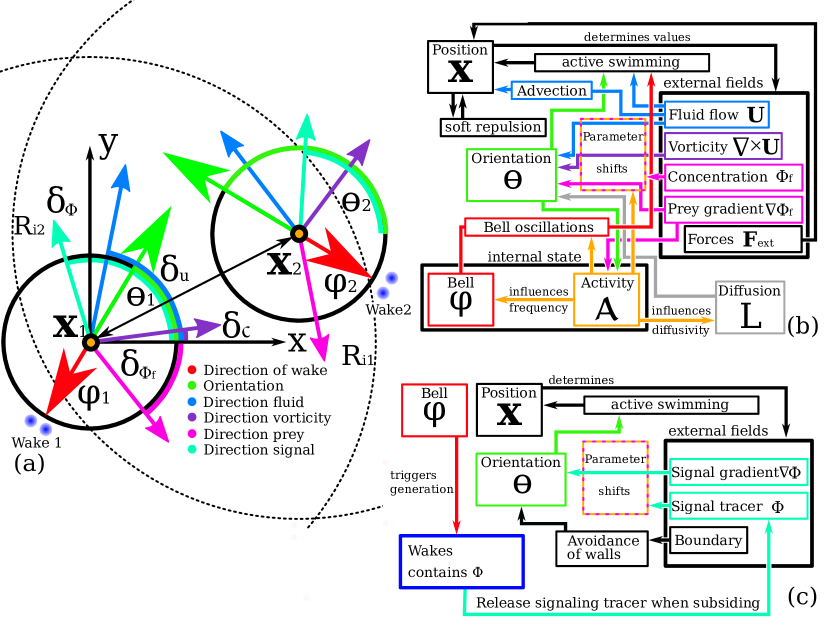
Figure 1: Depicted is a schematic of the jellyfish dynamics. (a): Schematics of agent-agent interaction and orientation inputs with colors corresponding to panel (b,c). The interaction radii $R_{i;1,2}$ are depicted by dashed lines. (b): The base model for jellyfish swarming, developed in [49]. This model considers only the passive external stimuli of a current $\mathbf{U}$ and the activating external stimulus of prey $\phi_{f}$ as drivers of pattern formation. (c): Augmentations of the model in panel (b) by self-induced signaling tracer coupling and turning near walls.

2.1.1 Bell Oscillations

Jellyfish possess a simplistic yet highly efficient neuronal net that is distributed over the bell. Its functional units often serve multiple purposes [59, 60, 61, 62, 25, 63]. We consider the fact that this network generates a macroscopic neuronal oscillation of the bell which we can represent by a phase, $\varphi_{j}$. Such a description still keeps essential features of the collective internal neuronal bell dynamics but reduces greatly the computational complexity [64, 65, 66, 67, 68]. In terms of the phase, the unperturbed bell dynamics is then given by

$$\dot{\varphi}_{j}=\omega_{j}=\Omega\;.$$ (1)

This equation states that the phase (of the bell) increases linearly because the bells oscillate approximately with a constant frequency, $\omega_{j}$, that can vary according to the size of individuals, species and seasons. Here, we assume a constant bell frequency of $\Omega$. The phase maps to different events in a pulsation cycle. Here, we adapt the convention that a closed bell is associated with a phase of $\varphi_{j}=2\pi m,m\in\mathds{N}$. (Hereafter we consider only the case $\phi_{j}=0$ due to symmetry.)

2.1.2 Wake Dynamics

Jellyfish eject wakes that consist of starting and stopping vortex rings and vortex super structures [69, 26, 70, 71]. The main thrust is produced when the bell contracts and closes, producing the starting vortex. In our model this corresponds to a bell phase of $\varphi=0$. We assume that the wake carries the tracer $\phi$ in its relatively coherent vortex structure. This vortex then subsides into the background turbulence where it releases the tracer. Here, we do not resolve this intermediate transport phenomenon explicitly. Instead, the tracer $\phi$ gets released immediately when the bell closes. This corresponds to the limit of infinitely large wake viscosity.

2.1.3 Positional Dynamics

We model the positional dynamics by

$$\dot{\mathbf{x}}_{j}=\mathbf{U}_{j}+V(\varphi_{j})\hat{e}_{j}(\theta_{j})+\frac{1}{N^{a}_{j}}\sum_{k\neq j}^{N^{a}_{j}}\mathbf{I}(\mathbf{x}_{k},\mathbf{x}_{j},\varphi_{k})+\mathbf{F}_{\text{ext}}\;.$$ (2)

It takes into account advection according to the background flow $\mathbf{U}_{j}=\mathbf{U}(\mathbf{x}_{j})$, volume exclusion and active swimming into direction $\theta_{j}=\text{arg}(\hat{e}_{j})$ with a speed

$$V(\varphi_{j})=\left(V_{0}+\frac{V_{1}|\mathbf{U}|}{V_{2}+|\mathbf{U}|}\right)\beta(\varphi_{j}),\qquad\beta(\varphi_{j})=e^{J_{v}(\cos(\varphi_{j})-1)}\;.$$ (3)

The function $\beta(.)$ mimics the pulsatile motion of jellyfish (see Fig. 2 panel (a)). Its shape depends on the parameter $J_{v}$. For large $J_{v}$, a jellyfish comes to a full stop in its bell cycle while for small $J_{v}$, an agent maintains a certain level of speed [49]. The additional nonlinear dependence of the velocity magnitude on the magnitude of the mean flow, $|\mathbf{U}|$ takes into account that jellyfish are able to swim faster against the direction of flow [29, 30]. The response is quasi-linear with slope $V_{1}/V_{2}$ at small flow velocities and it saturates at large flow velocities to $V_{1}$ [49]. Parameters of this mechanism are listed in Tab. 1

$N^{a}_{j}$ is the number of ABP-jellyfish found within a distance of $R_{i}$ around the jellyfish $j$. We model the interaction at short distances by a static and rotational symmetric repulsion

$$\mathbf{I}(\mathbf{x}_{j},\mathbf{x}_{k})=\frac{\mathbf{x}_{k}-\mathbf{x}_{j}}{|\mathbf{x}_{k}-\mathbf{x}_{j}|}-R_{i}\frac{\mathbf{x}_{k}-\mathbf{x}_{j}}{|\mathbf{x}_{k}-\mathbf{x}_{j}|^{2}}\;,$$ (4)

acting in between individuals $j$ and $k$ at distances $|\mathbf{x}_{k}-\mathbf{x}_{j}|<R_{i}$ [72, 73, 74] (see Fig. 2 panel (b)). At the edges of the computational domain, the walls repel agents by a reset force $\mathbf{F}_{\text{ext}}$.

Figure 2: Panel of coupling functions. (a): Phase dependence of the velocity magnitude Eq. (3) for parameters $J_{v}\in[5,1,0.5]$; (b): Radial dependence of the volume exclusion term in Eq. (4) for different interaction radii $R_{i}\in[0.15,0.5,1]$. Dashed lines indicate the omitted attractive part of the interaction; (i): Normalized coupling parameter $\varepsilon_{\phi}$ Eq. (9) for three sets of parameters $S_{\phi,1},S_{\phi,2}$.

2.1.4 Orientation Dynamics

The orientation of sparsely distributed jellyfish is affected only by environmental drivers and by the behavioral responses of individuals. To capture this effects, it suffices to consider the angular dynamics

$$\begin{aligned} \dot{\theta}_{j}&=L_{j}(t)+E(\mathbf{U}_{j},{\cal C}_{j},\phi_{f,j},\theta_{j})-\varepsilon_{\phi}(\phi)\sin(\theta_{j}-\delta_{\phi})+\pi\sin(\theta_{j}-\delta_{n,j}))K(\mathbf{x}_{j})\end{aligned}\;.$$ (5)

This dynamics is similar to that of an externally driven nonlinear oscillator with fluctuating frequency [66].

The fluctuation $L_{j}$ in Eq. (5) mirrors the effect of turbulence on the directional decision making of jellyfish (see Fig. 1 panel (b)). What stands behind this term is a neuro-mechanical feedback [71, 22] in which the turbulent fluid motion around a jellyfish causes a macroscopic tumbling. We assume this effect to be uncorrelated with other environmental drivers [75, 76, 77]. At the same time, a jellyfish induces the fluid motion such that the fluctuation $L_{j}$ is correlated in time. Accordingly, we model it by an Ornstein-Uhlenbeck process [78] following the dynamics

$$\dot{L}_{j}=-\lambda_{\theta}L_{j}+\eta(t),\qquad\langle\eta\rangle_{t}=0,\;\;\langle\eta(t)\eta(t^{\prime})\rangle_{t}=2D_{\theta}\delta(t-t^{\prime})\;.$$ (6)

Here, $D_{\theta}$ is the angular diffusion coefficient and $\lambda_{\theta}$ is the noise damping.

The behavioral effects of activating external stimuli, namely the flow field $\mathbf{U}_{j}$, the vorticity field ${\cal C}_{j}=\nabla\times\mathbf{U}_{j}$ and the distribution of prey (see Fig. 1 panel (a) and (b)) are taken into account by a phase coupling function, $E(.)$. In this study, we consider effects of flow and turbulence by

$$E(\mathbf{U},{\cal C},\theta_{j})=\varepsilon_{\mathbf{U}}(\mathbf{U})\sin(\theta_{j}-\delta_{\mathbf{U}})+\varepsilon_{{\cal C}}({\cal C})\sin(\theta_{j}-\delta_{{\cal C}})\;.$$ (7)

Herein, $\delta_{\mathbf{U}}=\text{arg}([U_{x},U_{y}])$ and $\delta_{\cal C}=\text{arg}([\partial_{x}|{\cal C}|,\partial_{y}|{\cal C}|])$ are the directions of flow and vorticity gradient. Pattern formation due to these external inputs has been previously studied in [49] and can be extended to salinity, temperature or solar insulation which are all common causes of pattern generation [79, 37].

However, once the fluid is quiescent, directional clues due to flow and turbulence are no longer present or they are ignored by a jellyfish ($E(.)\equiv 0$). This situation can be easily incorporated into the angular dynamics by a parameter response of the form

$$\varepsilon_{\mathbf{U}}(\mathbf{U})=\varepsilon_{\mathbf{U},0}{\cal T}(S_{\mathbf{U},1},S_{\mathbf{U},2},\mathbf{U}),\qquad\varepsilon_{{\cal C}}({\cal C})=\varepsilon_{{\cal C},0}{\cal T}(S_{{\cal C},1},S_{{\cal C},2},{\cal C}),\qquad{\cal T}(p_{1},p_{2},s)=\frac{1}{2}\Big{(}1+\tanh(p_{1}(s-p_{2}))\Big{)}\;.$$ (8)

The activation function ${\cal T}(.)$ is a reminiscence of neural field models [80, 81] which incorporate nonlinear saturation behavior of neurological responses. $\varepsilon_{0}$ is the reorientation strength. It is inversely proportional to its respective reorientation time scale. Parameter $p_{1}$ determines how sudden a reaction to a change in stimulus $s$ takes place and $p_{2}$ represents the sensitivity threshold for the stimulus (see Fig. 2 panel (c)). In behavioral terms, the parameters $S_{\mathbf{U},2}$ and $S_{{\cal C},2}$ set the intensity levels below which the activating external stimuli are ignored.

To model collective self-organized pattern formation, we consider a signaling tracer $\phi$ that is injected into the fluid by the jellyfish themselves (see Fig. 3 panel (a)). The corresponding phase coupling term of strength $\varepsilon_{\phi}$ causes each agent to orient into directions $\delta_{\phi}=\text{arg}([\partial_{x}\phi,\partial_{y}\phi])$. In our model, the strength of this interaction changes with the ambient signaling tracer concentration according to

$$\varepsilon_{\phi}(\phi)=\varepsilon_{\phi,0}{\cal T}(S_{\phi,1},S_{\phi,2},\phi){\cal T}(S_{\phi,1},S_{\phi,2}-1,-\phi)\;.$$ (9)

Here, we use the product of two threshold functions to account for a vanishing reaction at weak stimuli amplitudes, reflecting a low density of jellyfish on the one hand. On the other hand, when the jellyfish density, $\rho$ is high, the gradient-angle formulation should also break down as near-field agent-agent interactions gain importance. Here, we assume that the response is symmetric such that the lower and upper sensitivity are determined by $S_{\phi,2}$ (see Fig. 2 panel (c)).

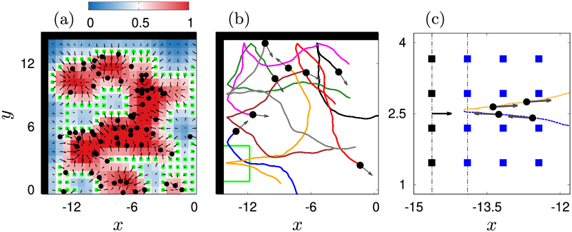
Figure 3: (a): Depicted is a snapshot of the upper left corner of the swarming domain for $D_{\phi}=0.001$ m² s^-1, $S_{\phi}=0.41$ corresponding to Fig. 7. Jellyfish are indicated by black dots and black arrows indicate the gradient of $\phi$. Green markers indicate the region where self-induced stimulus is affecting the behavior ($\varepsilon_{\phi}>0$). (b): Shown are example trajectories of jellyfish near the left and upper walls in the absence of chemotaxis ($\varepsilon_{\phi}=0$). The green box indicates a zoom to one of the turning events in panel (c). Four example positions of the agents are shown before and after the turning event, also indicated by the blue and orange part of its trajectory. Blue squares indicate fluid cells and black squares indicate the wall elements. The horizontal arrow pointing to the right indicates the wall normal $\hat{e}_{\text{wall}}$ corresponding to $\delta_{n}=0$.

In tank experiments, jellyfish are faced with a considerable problem: They have to avoid walls to preserve their fragile bodies. However, their persistence time $\tau_{p}=\lambda_{\theta}^{2}/D_{\theta}$ and persistence length $L_{p}=\langle V\rangle\tau_{p}$ are roughly $\tau_{p}\sim 250$ s and $L_{p}\sim 17$ m [30, 49, 82, 83]. Thus, their free swimming paths are frequently interrupted by walls in most tank-based experiments! The time scale at which a wall avoidance takes place should be of the order $2R_{i}/\langle V\rangle\sim 4$ s [30] in this study! Thus, turning at walls must be of active nature. A simplistic approach to include such a response is to include angular coupling relative to the wall normal $\hat{e}_{\text{wall}}$ with direction of $\delta_{n,j}=\text{arg}(\hat{e}_{\text{wall}})$. We consider a relatively fast rotation rate of $\pi K(\mathbf{x}_{j})$ rad s^-1 which causes a full reflection to last for $1$ s. This wall interaction sets in only when an agent is near a wall. We model this by a Boolean mapping $K(\mathbf{x}_{j})$. (see Fig. 3 panels (b,c) and App. A).

2.1.5 Tracer Dynamics

The signaling tracer in the fluid evolves according to the advection-diffusion equation

$$\frac{D\phi}{Dt}=-D_{\phi}\Delta\phi+{\cal S}\;.$$ (10)

Here, $D/Dt\equiv\partial_{t}+U_{x}\partial_{x}+U_{y}\partial_{y}$ is the horizontal advective derivative and $D_{\phi}$ is the diffusion constant of $\phi$ [84]. It determines how much structural details are smoothed out. The forcing term is

$${\cal S}(\rho,\gamma)=C_{\phi}\text{Coupling}(\rho)-\Gamma\cdot(\phi),\qquad\int\text{Coupling}(\rho(\mathbf{x}))d\mathbf{x}=N\;.$$ (11)

In our model the source is resembled by superposition of Gaussian bell curves tied to $N$ discrete jellyfish positions. These positions correspond to the jellyfish area density $\rho$. The amplitude of the source is given by the mixing factor $C_{\phi}=\text{Volume}_{\text{bell}}/\text{Volume}_{\text{cell}}$ which is defined by the ratio of grid cell volume and bell fluid volume. $C_{\phi}$ is essentially a free parameter, determined by the vertical depth of a grid cell and the bell physiology (see Sec. 2.4). The coupling of the tracer to the fluid grid assumes an initial diffusive mixing due to the presence of wakes. We model a simplistic exponential sink term with a decay constant $\Gamma$. The sink models the effect of sedimentation, vertical advection or microbial consumption.

2.2 Numerical Simulation

The dynamics of ABP-jellyfish is simulated using the stochastic Heun method [85]. The Diffusion of tracers Eq. (10) and the fluid flow are simulated on a staggered grid with $41\times 41$ grid points spanning a quadratic area of $30\times 30$ m (grid 1) or $90\times 90$ m (grid 2). We solve the Navier-Stokes equation for a density of $\rho_{f}=1000$ kg $m^{-3}$ and an effective viscosity of $\mu=2$ Ns m^-2 on grid 2 (see Sec. 3.4). The agent time step is set to $0.01$ s. Data is collected every $0.5$ s. We use a tri-linear spatio-temporal interpolation to resolve field values onto the coordinates of the agents at time $t$ [86]. The Gaussian coupling functions in Eq. (11) have spreading radii of $R_{s}=1$ m (grid 1) and $R_{s}=2$ m (grid 2).

2.3 Statistical Analysis

We make use of the following statistical quantities:

$${\cal R}_{n} = \sqrt{\langle\langle r^{2}\rangle_{n}\rangle_{N}},$$       Local mean-square distance (12)

$$\text{Hex}_{m} = \langle|\langle\exp{i6\delta}\rangle_{m}|\rangle_{N},$$       Hexagonal order parameter

$$\Phi = \frac{\langle\phi\rangle_{N}}{\langle\phi\rangle_{\text{tank}}},$$       Tracer ratio

$${\cal N} = \langle K\rangle,$$       Average cluster size

Herein, $\langle.\rangle$ denotes ensemble averages. Lower case indices denote average over the $n$ and $m$ nearest neighbors and index $N$ indicates averaging over all agents. For ${\cal R}_{n}$ and Hex_m we adapted a two-stage averaging since the swarm generally consists of several, disconnected, clusters (see Fig. 5 panels (b-e)). ${\cal R}_{n}$ and Hex_m are additionally normalized by their values near $t=0$. We average our model results over $M$ runs and locally over time, using a Gaussian kernel-density smoother with a time window of $20$ s. For the local ensemble averages we use the $n=6$ and $m=24$ nearest neighbors. In the following, we drop these indices for simplicity.

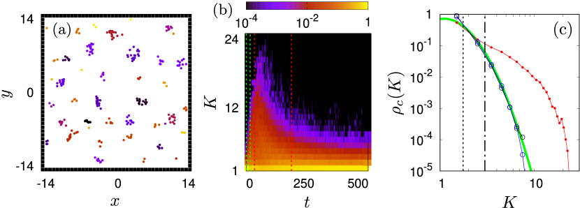
Figure 4: (a): Depicted is an exemplary decomposition of a jellyfish swarm into sub clusters for $R_{c}=0.5$ m. Dots of same color belong to the same cluster. The snapshot is taken at $100$ s from the dynamics in Fig. 7 for $S_{\phi,2}=0.01$, $D_{\phi}=0.001$ m² s^-1. (b): Shown is the intermittent behavior of the CSD (color) over time. The green and red dashed vertical lines indicate the time intervals from which the averaged CSDs and ${\cal N}$ are obtained. Color coding indicates the average of $\rho_{c}(K)$ from $16$ model runs. (c). Shown are the CSDs $\rho_{c}(K)$ for averaging intervals $0<t<10$ s in black (green dashed lines in (b)) and $30<t<200$ s in red (red dashed lines in (b)). Additionally $\rho_{c}(K)$ in an interval $800<t<900$ s (blue) almost overlaps with the CSD in the beginning of the simulation (black). The bold green line indicates the log-normal distribution having standard deviation $0.45$ and mean $0.3$. Dashed and dashed-dotted vertical lines indicate ${\cal N}$ prior/after and during cluster formation respectively (see Fig. 6 panel (d)).

The local mean square distance, ${\cal R}$, measures the average distance of nearest neighbors. It thus indicates when jellyfish swim closer to each other [87, 88]. The hexagonal order parameter, Hex, measures the local hexatic-order in the swarm. It varies between zero (disorder) and unity (perfect hexatic order in an infinite system) [89, 90]. The tracer ratio is an indicator for the search success of the swarm. It measures the excess of the ambient tracer concentration in the swarm, $\phi_{J}=\langle\phi\rangle_{N}$ in comparison to the averaged tracer concentration in the tank, $\phi_{\text{tank}}=\langle\phi\rangle_{\text{tank}}$. The average cluster size, $\cal N$, is given by the first moment of the cluster-size distribution (CSD), $\rho_{c}(K)$. The CSD is calculated according to a geometric interaction radius $R_{c}$: If $K$ ABP-jellyfish form a geometric graph in which each link is shorter than $R_{c}$, they belong to the same cluster of size $K$ (see Fig. 4 (a)) [91, 92]. We average the CSD over $M$ model runs and over different time intervals (see Fig. 4 (b,c)). We denote the respective run-ensemble-time averages of all quantities in Eq. (12) by an overbar.

2.4 Parameter Settings

The interaction dynamics of jellyfish is specified by $20$ parameters which are listed in Tab. 1. We use here an interaction radius of $R_{i}=0.15$ m, in contrast to [49] where $R_{i}=0.1$ m. Our intention is to allow for a larger sphere of influence while keeping in mind that the bell diameter is given by $R_{\text{min}}=0.1$ m.

Parameter, [unit]	Value	Process	Parameter, [unit]
$R_{i}$, [m]	$0.15$
$V_{0}$, [m s-1]	$0.15$	Active swimming
$J_{v}$, [-]	$1$
$V_{1}$, [m s-1]	$0.5$
$V_{2}$, [m s-1]	$0.6$
$S_{\mathbf{U},1}$, [s m-1]	$400$
$S_{\mathbf{U},2}$, [m s-1]	$0.03$
$\varepsilon_{\mathbf{U},0}$, [rad s-1]	$0.16$
$S_{{\cal C},1}$, [s rad-1]	$400$	Avoidance of turbulence
$S_{{\cal C},2}$, [rad s-1]	$0.005$
$\varepsilon_{{\cal C},0}$, [rad s-1]	$0.08$
$\Omega$, [rad s-1]	$7.54$	Bell pulsation
$\lambda_{\theta}$, [s-1]	$-5$	Orientation dynamics	$\varepsilon_{\phi,0}$, [rad $s^{-1}$]
$D_{\theta}$, [rad2 s${-3}$]	$0.1$		$S_{\phi,2}$, [$F_{0}$]
$S_{\phi,1}$, [$F_{0}^{-1}$]	$400$
$C_{\phi}$, [-]	$0.0083$ (grid 1)	Signaling diffusion	$D_{\phi}$, [m2 s-1]
	$0.00031$ (grid 2)		$\Gamma$, [s-1]

Table 1: Listing of model parameters. The central column indicates the process in the model. The left column list parameters that are fixed in this model. The right columns list free parameters investigated in this study.

The mixing factor $C_{\phi}$ follows from the assumptions that grid cells are cubes and the jellyfish bell has spherical shape. Then, $\text{Volume}_{\text{bell}}\sim R_{\text{min}}^{3}$. According to in-situ measurements of the wake volume [26], where $3\text{Volume}_{\text{bell}}=1213\cdot 10^{-6}$ m³ (for $R_{\text{min}}=0.05$ m) we extrapolate a mixed bell volume (for $R_{\text{min}}=0.1$ m) $\text{Volume}_{\text{bell}}=1213\cdot 10^{-6}8/3$ m${}^{3}=0.0032$ m³. This results in mixing factors for grid 1: $\text{Volume}_{\text{cell}}=(30/41)^{3}$ m${}^{3}\Rightarrow C_{\phi}=0.0083$ and for grid 2: $\text{Volume}_{\text{cell}}=(90/41)^{3}$ m${}^{3}\Rightarrow C_{\phi}=0.00031$.

3 Results

We first consider the situation of a quiescent fluid ($\mathbf{U}=0$) without a tracer sink ($\Gamma=0$). The dynamics Eqs. (1-11) in this case still features the free parameters $\varepsilon_{\phi,0}$, $S_{\phi,1}$, $S_{\phi,2}$ and $D_{\phi}$. At this point, we fix $S_{\phi,1}=400$ such that the decoupling from the tracer gradient according to Eq. (9) is almost instantaneous at respective $S_{\phi,2}$ (see Fig. 2 panel (c)). We first consider a smaller tank with $900$ m² area (grid 1) and simulate the dynamics of $N=256$ jellyfish which start in a square of $28\times 28$ m² ($\rho(0)=N\pi R_{i}^{2}/28^{2}=0.023$). We average results here over $16$ model runs.

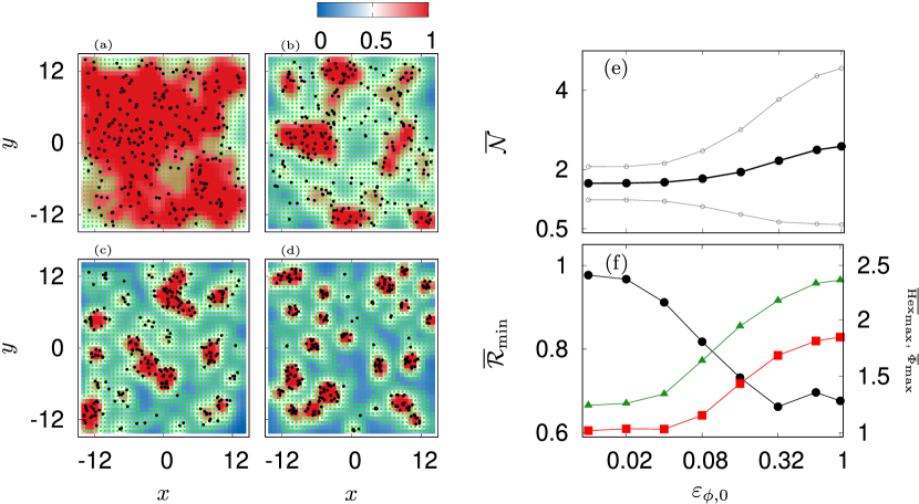
Figure 5: Depicted is the dependence of jellyfish clustering on the orientation strength $\varepsilon_{\phi,0}$. (a): $\varepsilon_{\phi,0}=0.01$ rad s^-1. (b): $\varepsilon_{\phi,0}=0.04$ rad s^-1, (c): $\varepsilon_{\phi,0}=0.16$ rad s^-1, (d): $\varepsilon_{\phi,0}=0.64$ rad s^-1. (e): Shown is the average cluster size (black) with its standard deviation (grey) for a geometric interaction radius $R_{c}=0.5$. m. (f): Shown is the dependence of the minimal local agent-agent distances ${\cal R}_{\text{min}}$ (black dots, left axis) and the maximal hexagonal order of the ABP-jellyfish (red squares, right axis) and the maximum ratio of the signaling tracer concentration $\Phi$ (green triangles, right axis). Other model parameters are $S_{\phi,2}=0.17$, $D_{\phi}=0.01$ m² s^-1.

3.1 Coupling Strength

The coupling strength $\varepsilon_{\phi,0}$ determines how fast ABP-jellyfish turn towards the $\phi$-gradient. In Fig. 5 exemplary snapshots are depicted. For weak coupling, the ABP-jellyfish remain effectively uniformly distributed throughout the simulation while stronger angular couplings evoke amplification of small density fluctuations and thus, formation of successively more and more pronounced and disconnected patches. This parameter response is reflected by an increase of the average cluster size, ${\cal N}$ (Fig. 5 panel (e)), a decrease in the minimal average agent-agent distance, ${\cal R}_{\text{min}}$, and an increase in the maximum values of hexagonal order, Hex${}_{\text{max}}$, and tracer ratio, $\Phi_{\text{max}}$ (Fig. 5 panel (f)). In this setting, we observe that the ABP-jellyfish groups are dissolved after formation because $\phi$ gets enriched in the absence of a sink. Accordingly, we use the extreme values of ${\cal R}$, Hex and $\Phi$. For the same reason, the average cluster size was obtained during the clustering period ranging from $30$ s to $200$ s (see Fig. 4).

3.2 Tracer and Clustering

The tracer dynamics is of further interest. In fact, since we have not included a tracer sink for now ($\Gamma=0$), $\phi$ increases linearly with a rate

$${\cal J}=C_{\phi}\frac{\rho}{\pi R_{i}^{2}}\frac{\Omega}{2\pi}\;,$$ (13)

when the ABP-jellyfish are uniformly distributed (see Fig. 5 panel (a)). Exemplary transients of $\phi_{J}$ and $\phi_{\text{tank}}$ are shown in Fig. 6 panel (a). There, both, $\phi_{J}$ and $\phi_{\text{tank}}$ rise almost linearly with a rate ${\cal J}=0.003$ s^-1 prior to patch formation. However, after approximately $100$ s, the swarm concentration, $\phi_{J}$, increases more rapidly because jellyfish converge towards local fluctuations of $\rho$ and the tank concentration, $\phi_{\text{tank}}$, crosses over to a more modest growth rate, governed by diffusive transport of $\phi$ to regions between patches and release of tracer by solitary jellyfish. After careful checking of our results, we found that most of the density collapse takes place before the linear saturation time $\tau_{\text{sat}}={\cal J}^{-1}$ as can be seen by a comparison of the range of clustering times $\tau^{\star}_{\cal R}$ (red dashed vertical lines in Fig. 6 panel (a) and solid lines in panel (c)).

We further tested the dependence of patch formation on $D_{\phi}$. Generally, the diffusivity is inversely proportional to a time scale of structural smoothing and thus, influences how fast patches can merge. We see in Fig. 6 panel (b) that ${\cal R}_{\text{min}}$ is inversely proportional to $D_{\phi}$. The reason for this is that under fast structural smoothing small clusters or solitary jellyfish are almost always absorbed into larger clusters. In contrast, weak diffusion hampers the growth of patches such that solitary medusae or small clusters are more likely. In this case, averages over the $n$ nearest jellyfish become non-local and take into account members of other clusters (compare snapshots Fig. 7). ${\cal R}_{\text{min}}$ mostly scales $\sim S_{\phi,2}$ at low sensitivities ($S_{\phi,2}\rightarrow 0.5$). Interestingly, at very high sensitivities ($S_{\phi,2}\rightarrow 0$) ${\cal R}_{\text{min}}$ is quasi independent of $S_{\phi,2}$, indicating that cluster formation is driven by fluctuations of density $\rho$ rather than behavioral sensitivity. Our simulations show that ${\cal R}_{\text{min}}$ is approached at different times $\tau^{\star}_{\cal R}$, after the maximal tracer ratio was reached (see Fig. 6 panel (c) where $\tau^{\star}_{\cal R}>\tau^{\star}_{\Phi}$). We attribute the spread of $\tau^{\star}_{\cal R}$ to the process of cluster merging when the clusters are initially quite small.

Finally, the average cluster size, ${\cal N}$, indicates that the largest clusters form for small $S_{\phi,2}$ (see Fig. 6 panel (d)) and that clusters become bigger when tracer spreads out more rapidly according to larger $D_{\phi}$. When $S_{\phi,2}\rightarrow 0.5$, ${\cal N}$ approaches the cluster sizes found in the quasi-random ensembles at simulation start and end (black square-dashed lines in panel (d)). $\overline{\cal N}$ is obtained from time averages of the CSD, $\rho_{c}(K)$, in intervals $0$ s $<t<10$ s (simulation start), $30$ s$<t<200$ s (clustering period), $800$ s $<t<900$ s (simulation end).

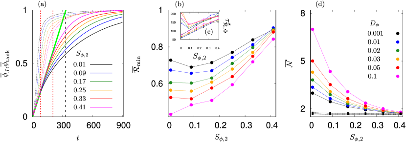
Figure 6: (a): Depicted are the averaged transients for the averaged concentration of agents, $\phi_{J}$ (dashed lines) and in the tank $\phi_{\text{tank}}$ for different sensitivities $S_{\phi,2}$ and diffusivities $D_{\phi}=0.001$ m² s^-1, $\varepsilon_{\phi,0}=0.32$ rad s^-1. The green line indicates the slope ${\cal J}=0.003$ s^-1. the vertical black dashed line indicates $\tau_{\text{sat}}$ and the red lines indicate the range of all the clustering times $\tau^{\star}_{\cal R}$. (b): Shown is the dependence of the minimal local mean square distance, ${\cal R}_{\text{min}}$ on $S_{\phi,2}$ and $D_{\phi}$. The inserted panel (c) depicts the clustering times $\tau^{\star}_{\cal R}$ (bold lines, dots) and the times, $\tau^{\star}_{\Phi}$, when the tracer ratios $\Phi$ reach their maximum (dashed lines, squares). (d): Shown is the averaged cluster size $\overline{\cal N}$ during the clustering period, depending on $S_{\phi,2}$ and $D_{\phi}$ for $R_{c}=0.5$ m.

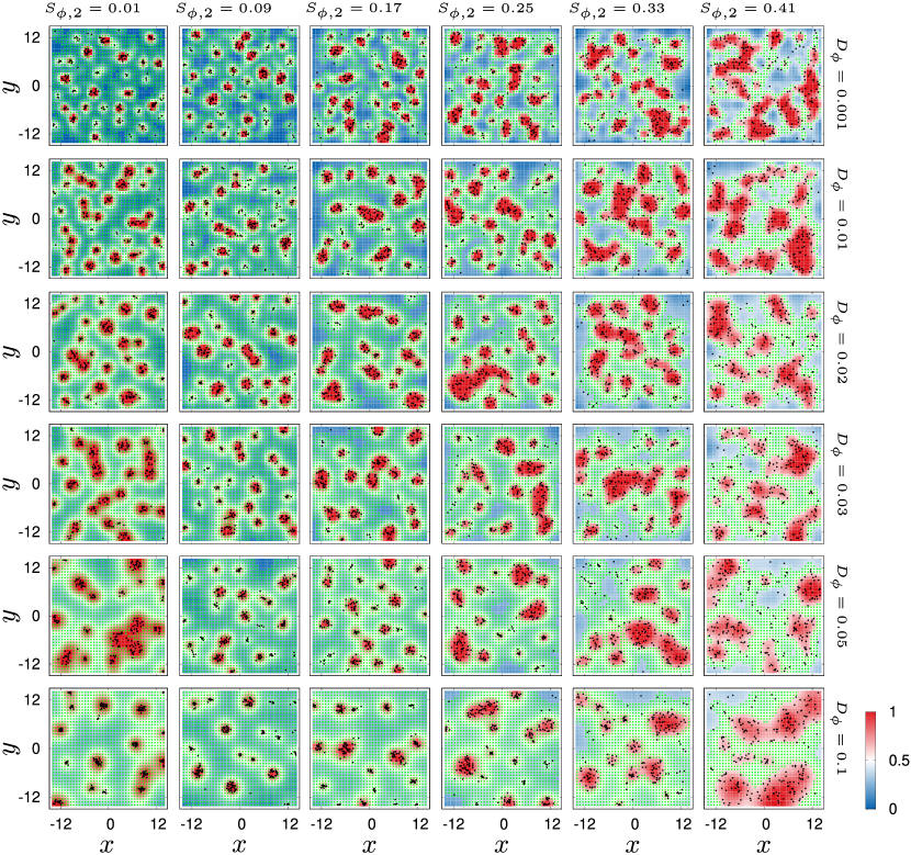
Figure 7: Depicted are snapshots of the patch structures at clustering times $\tau^{\star}$ corresponding to points in Fig. 6 panel (b,c). The angular coupling strength is $\varepsilon_{\phi,0}=0.64$ rad s ^-1. Color maps indicate $\phi$. Black dots indicate the ABP-jellyfish. Regions where the self-induced stimulus affects the angular dynamics are indicated by a green raster.

3.3 Effect of a Tracer Sink

Now, we investigate the effect of a tracer sink ($\Gamma>0$) on patch formation, based on the full diffusion dynamics Eq. (10). For a uniform tracer field and uniformly distributed jellyfish, spacial averaging yields the tracer concentration

$$\phi_{\text{tank}}(t)=\frac{{\cal J}}{\Gamma}\left(1-\exp(-\Gamma t)\right)\;.$$ (14)

It is immediately clear that the saturation value $\phi^{\star}={\cal J}/\Gamma$ potentially lies below the threshold value $S_{\phi,2}$ effectively preventing the onset of patch formation. Moreover, the characteristic time scale for tracer dynamics is now $\tau^{\prime}_{\text{sat}}=\Gamma^{-1}$. To discuss a relevant example, we divert our investigations now to a larger tank of $90\times 90$ m² with $N=1024$ jellyfish started in a square of $72\times 72$ m². These settings result in $\rho(0)=0.014$, ${\cal J}=0.000073$ s^-1, $\tau_{\text{sat}}\approx 4$ h. We consider here fixed parameters $D_{\phi}=0.001$ m² s^-1 and $S_{\phi,2}=0.03$. The critical sink strength is thus given by $\Gamma_{\text{crit}}={\cal J}/S_{\phi,2}=0.00245$ s^-1 (vertical dashed line in Fig. 8). We run each model instance for $7200$ s and average our results over $4$ runs.

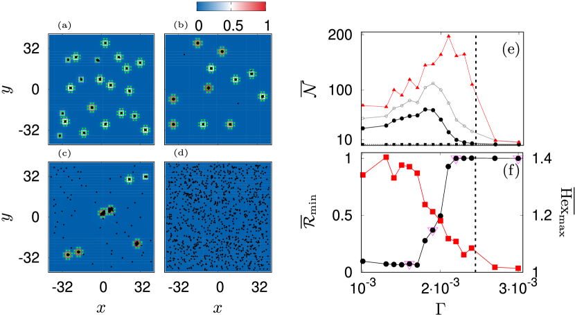
Figure 8: Depicted are snapshots of the swarms at $t=7200$ s, similar to Fig. 5. (a): $\Gamma=0.0016$ s^-1, (b): $\Gamma=0.0019$ s^-1, (c): $\Gamma=0.0022$ s^-1, (d): $\Gamma=0.003$ s^-1 (pink triangles in panel (f)). Other parameters of the simulation are $\varepsilon_{\phi,0}=0.32$ rad s^-1, $D_{\phi}=0.001$ m² s^-1, $S_{\phi,2}=0.03$. Shown in panel (e) is the average cluster size $\overline{\cal N}$ (black dots) with its upper standard deviation (grey circles) and the average cluster size in the $95\%$ percentile of $\rho_{c}(K)$ (red triangles) $R_{c}=1$ m. Panel (f) presents the maximal hexagonal order parameter, Hex${}_{\text{max}}$ (red squares, right axis), and the minimal local mean square distance, ${\cal R}_{\text{min}}$ (black dots, left axis). The dashed vertical line indicates $\Gamma_{\text{crit}}$.

An increase of sink strength, $\Gamma$, causes successively less patches to form, indicating a clustering transition (see Fig. 8 panels (a-d)). In fact, this transition takes place at lower values than $\Gamma_{\text{crit}}$ which here can be attributed to a slight expansion of the swarm into the whole tank, thus decreasing ${\cal J}$. Largest clusters emerge near $\Gamma_{\text{crit}}$ (see Fig. 8 panels (e)). However, even at sink strength as high as $\Gamma=0.0027$ s${}^{-1}>\Gamma_{\text{crit}}$ clusters can be observed within our simulated time. Similarly to results of Sec. 3.1, we see that fluctuations of cluster size are largest near the clustering transition. This becomes particularly clear if we observe the largest clusters, indicated by the $95\%$ percentile of $\rho_{c}$ (red triangles in Fig. 8 panel (e)). A comparison of panels (e) and (f) shows that ${\cal R}$, Hex and ${\cal N}$ indicate different transition points $\Gamma_{\text{crit}}$. In case of ${\cal R}$, panels (c,d) in Fig. 8 indicate that a few remaining solitary jellyfish dominate the averaging procedure. On the contrary, Hex shows a much more gradual transition, However, we carefully checked our results and found that Hex shows an intermittent behavior over time. While first increasing, Hex decreases in the long run. Since we used $24$ nearest neighbors to calculate Hex, we attribute this behavior to the formation of small clusters and the continued pulsatile motion of individuals even inside clusters.

3.4 Interplay of activating external Stimuli and a self-induced Stimulus

Up to this point we have discussed structure formation in the presence of a self-induced stimulus, $\phi$. However, it will always act in concert with external stimuli, in particular in the open sea. Thus, we here elaborate on the emergence of jellyfish patches in a flow ($\mathbf{U}\neq 0$). For this, we consider the commonly encountered experimental setting of an inflow current (see Fig. 9). Confronted with such a setting, jellyfish will not just consider the self-induced signaling corresponding to $\phi$ but rather consider also activating external stimuli which in our model are the flow $\mathbf{U}$, and the absolute vorticity, $|{\cal C}|$ which we use as a measure of turbulence. We use the larger tank (grid 2) and drive the fluid with an inflow current of $0.1$ m s^-1. The outflow is situated in the lower right of the tank. This configuration leads to the formation of a strong jet that separates the tank. Left of the current, a narrow quiescent region and a smaller but strong vortex are found. Right of the current, a large counter-clockwise rotating vortex exists. The upper right part of the tank is relatively quiescent (Fig. 9 panel (a)). The parameters levels $S_{\mathbf{U},2}$ and $S_{{\cal C},2}$ separate the flow domain into several distinct regions (see Fig. 9 panel (b)). We fix here $S_{\mathbf{U},2}=0.03$ m s^-1 such that the ABP-jellyfish counter the current inside the jet and in the branching helices of the vortices. And we let $S_{{\cal C},2}=0.005$ rad s^-1 such that turbulence avoidance is mostly present in the edges of the jet (triangles and squares in Fig. 9 panel (b)).

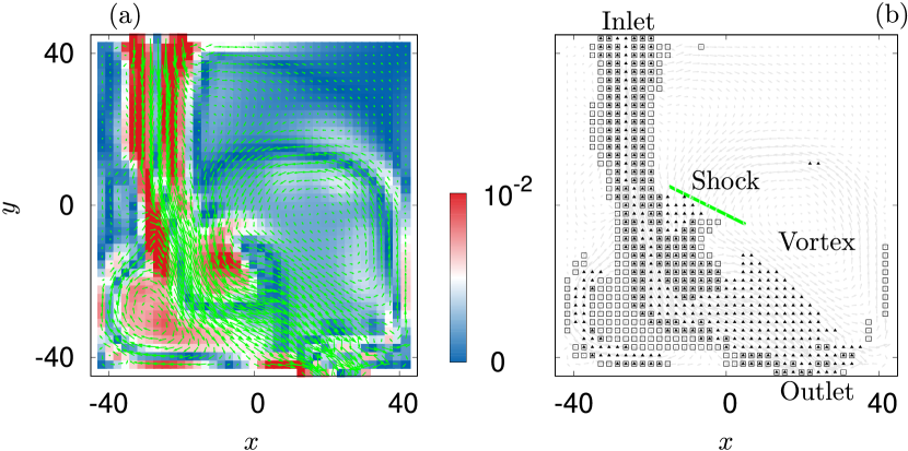
Figure 9: (a): Depicted are typical flow field $\mathbf{U}$ (green arrows) and the absolute vorticity $|{\cal C}|$ (colors) at $4800$ s. (b): Shown with markers are the decision regions. Triangles indicate regions of counter-current swimming for $S_{\mathbf{U},2}=0.03$ m s^-1 and boxes indicate regions of turbulence avoidance for $S_{{\cal C},2}=0.005$ rad s^-1. The green line indicates the position of the turning shock where clusters are formed.

If the angular dynamics is decoupled from $\phi$, counter-current swimming and vorticity avoidance cause many jellyfish to group in front of the inlet. The transient structure towards this cluster is a long filament (Fig. 10). In fact, the turbulence avoidance acts like a wall and focuses the jellyfish inside the jet. An other large group instead remains for a long time in the quiescent region of the upper right. This behavior of jellyfish is reflected in the time-averaged distribution $\overline{\rho}=\overline{\langle\rho(\mathbf{x})\rangle_{t}}$, depicted in panel (d 1) of Fig. 10. There, we clearly see that the jet cluster is the most pronounced feature besides a large density plateau in the upper right of the tank.

Notably, we observe the tendency of jellyfish to form a loose conglomerate in the center of the tank. The reason for this is a turning shock, where the upper helix of the main vortex joins the jet again (green line in Fig. 9 panel (b)). There, jellyfish are transported passively from the right into the jet region. Once inside the jet, they orient against the current such that they encounter more jellyfish that get transported by the helix flow into that region, causing a convergence of medusae. At some point, the emerging cluster falls apart and the jellyfish get transported further downstream (see Fig. 10 panels (a 1 - a 6)).

Once we also incorporate orientation due to $\phi$, clusters form and are indeed also maintained (compare Fig. 10 panels (a 1 - a 6) and (b 1 - b 6)). The area density of these clusters depends on $\varepsilon_{\phi,0}$ (see Fig. 10 panels (c 1 - c 6)). In fact, $\overline{\rho}$ allows us to identify regions in the flow that are likely to host clusters (see Fig. 10 panels (d 1 - d 6)). We make the following observations:

• Turning shock: Jellyfish get enriched in the region of the turning shock. When they orient due to $\phi$, they can form a structurally stable patch that gets transported downstream with the flow (coil structure in the center of panels (d 3 - d 6)).

• Vortex center: The coil structure near the turning shock does not extend or smear out to the right edge of the tank. The reason for this is that $\phi$ gets enriched in the quiescent central region of the main vortex where jellyfish then tend to stay due to the attractive action of $\phi$.

• Focus and distraction: The strong main current causes the ABP-jellyfish to focus in an equilibrium point where the active swimming of single individuals gets hampered due to non-synchronous pulsation of the bells inside the cluster. The cluster as a whole is then unable to overcome the background flow. Stronger coupling to $\phi$, causes the cluster inside the jet to become less prominent because individuals get distracted from their counter-current swimming by orientation towards $\phi$.

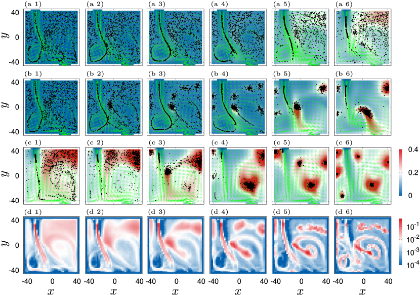
Figure 10: Depicted are swarming behaviors of ABP-jellyfish. Green arrows indicate the flow field. Colors in (a 1 - c 6) indicate $\phi$. Panels (a 1 - a 6) show the swarming behavior of the ABP-jellyfish when $\varepsilon_{\phi,0}=0$ and (b 1 - b 6) shows the swarming transient for $\varepsilon_{\phi,0}=0.03$ rad s^-1. Snapshots are taken at (ab 1): $300$ s, (ab 2): $600$ s, (ab 3): $900$ s, (ab 4): $1200$ s, (ab 5): $3600$ s, (ab 6): $4800$ s. Succession of panels (c 1 - c 6) shows the swarm in the end of the simulation at $7200$ s. (c 1): $\varepsilon_{\phi,0}=0$, (c 2): $\varepsilon_{\phi,0}=0.01$ rad s^-1, (c 3): $\varepsilon_{\phi,0}=0.02$ rad s^-1, (c 4): $\varepsilon_{\phi,0}=0.04$ rad s^-1, (c 5): $\varepsilon_{\phi,0}=0.08$ rad s^-1 and (c 6): $\varepsilon_{\phi,0}=0.16$ rad s^-1. Panels (d 1 - d 6) show the corresponding averaged jellyfish densities $\overline{\rho}$.

4 Discussion

The previous results suggest that the self-organized formation and maintenance of jellyfish blooms is subject to a plethora of environmental and behavioral factors. This can be best understood from Eqs. (13, 14) which combine external ($\Gamma$, $\rho$) structural ($\rho$), physiological ($C_{\phi}$, $R_{i}$, $\Omega$) and behavioral ($S_{\phi,2}$, $\Omega$, $\varepsilon_{\phi,0}$) aspects of the clustering transition. The main finding of the analysis is that external ($\mathbf{U}$, $|{\cal C}|$, $\Gamma$) and self-induced ($\phi$) stimuli both influence the swarming transition. The external drivers induce the transition by their effect on the jellyfish density, $\rho$ and the self-induced tracer $\phi$ is responsible for swarm maintenance. Accordingly, several scenarios are conceivable that lead to jellyfish blooming in the sea or formation of dense swarms in tanks:

• A regional or local convergence of currents causes $\phi$ to surpass the behavioral sensing threshold $S_{\phi,2}$. Alternatively, the local current, $\mathbf{U}$ or other activating external drivers such as the abundance of prey can cause a local increase of jellyfish density according to which the local tracer flux ${\cal J}$ increases, leading to swarm coherence (turning shock in Fig. 10) which then acts as a nucleus for swarm formation.

• Jellyfish can also cluster mutually as a consequence of volume exclusion, once the density is high enough. In that case, jellyfish start to feel each other and slow down in particularly dense regions. This leads to an effectively negative swimming pressure, forcing more and more jellyfish into structural collapse [93]. This scenario might be relevant within already formed patches where a stimulus like $\phi$ is maxed out, or when environmental conditions change on time scales much larger than the time scale of active swimming. For example, if $\langle V\rangle=0.067$ m s^-1 [30], converging on the scale of a kilometer requires a calm sea for approximately $4$ h, opting for night-time conditions in which such an effect might be observable. Alternatively this effect could be of interest for closed habitats like Lake Palau [94] and in tank experiments [54].

• Jellyfish can change the rate of tracer release, $C_{\phi}$ according to their life stage and season. Above, we also indicated that the mixing factor $C_{\phi}$ is sensitive to the effective fluid volume into which the tracer is released. Consequently, a direct influence of marine topography on blooming could be of relevance [27]. On shortest time scales, the mixing of tracer into the fluid depends on kinematic parameters like $\Omega$, the bell shape and the form of wakes.

• The interplay of sensing thresholds $S_{\mathbf{U},{\cal C},\phi;2}$ influences which $\phi$ concentration triggers the clustering instability described in this study. We have shown that the clustering transition takes place in a quite narrow range of small valued parameter (either $\Gamma$ or $S_{\phi}$), in accordance with the observation that jellyfish are extremely sensitive to changes in their environment [58]. On the one hand, such sensitivity certainly can be attributed to the process of natural selection [37]. On the other hand, we have seen in Sec. 3.1 that the clustering response at very high sensitivities (${\cal S}_{\phi}\rightarrow 0$) depends mainly on the diffusivity $D_{\phi}$, emphasizing the importance of externally induced density fluctuations on cluster formation. This suggest a less strict evolutionary corridor for the development of a certain high sensitivity because shock regions like in Fig. 10 are a common feature in many flow settings.

A particularly interesting observation of our simulations is that the largest patches of jellyfish emerge near the clustering threshold $\Gamma_{\text{crit}}$. In those simulations, the balance of tracer sink and induced tracer fluctuations is so delicate that the emergence of a single cluster suffices to deprive its surrounding of jellyfish. Consequently, the tracer levels in the domain around a cluster drop and remain below $S_{\phi,2}$ while the cluster itself becomes a strong source of $\phi$ that eventually incorporates the remaining freely swimming jellyfish. This seems to be a reflection of the actual swarm recruitment process in the calm sea or in bays and estuaries which indeed has a strong horizontal swimming component [95, 58]. Our analysis suggests that larger clusters are quite naturally favored over smaller ones. For this effect to be visible, the initial density of spread out jellyfish needs to be already high enough for local density fluctuation to reach the clustering threshold. Field observations are needed to check this hypothesis on proper spacial scales and by mimicing different stimuli.

While still just based on a simplified model of the actual biological reality, the clustering transition discussed here can be induced by a plethora of different model processes at time scales $\tau_{\text{sat}}={\cal J}^{-1}$ and $\tau_{\text{sat}}^{\prime}=\Gamma^{-1}$ (tracer-density fluctuation), $\varepsilon^{-1}_{\phi,0}$ (reorientation) and $D^{-1}_{\phi}$ (tracer transport), suggesting that the actual mechanistic complexity is the bio-physical ace of jellyfish which allows them to exploit different and relatively abundant conditions for bloom formation and to increase energy efficiency. In our simulations the latter is reflected by a distraction from the inlet jet current and by clustering inside the main vortex where flow velocities are small.

We deliberately do not specify what kind information is transported with $\phi$ because observational evidence for kinematic alignment according to pressure waves and wakes or tracer-oriented swimming is lacking. However, the evolutionary success of diffusive communication is well known: Bacteria use diffusing signaling molecules to communicate [96] and ant colonies are known to assemble large milling patters based on pheromone marking [97, 98]. In fact, jellyfish seem to resemble some properties also found in micro swimmers as they, have limitations in their physiology and feature a rotational persistence number, Pe$=L_{p}/(2R_{\text{min}})\sim 85$ [49] comparable to that of bacterial swimmers (Pe$\sim 10$) [77, 99, 100]. At the same time they are as big as fish!

Our analysis is based on the three quantities, ${\cal R}$, Hex and ${\cal N}$ (see Eq. (12)). Of these three, ${\cal N}$ is the most stable and universal indicator for cluster formation. Instead, ${\cal R}$ and Hex put a focus on specific aspects of clustering: ${\cal R}$ is affected by the presence of solitary jellyfish which, due to their non-local connections, shadow clustering effects, causing an abrupt transition of ${\cal R}$. Instead, Hex measures the degree of structural order and is affected by finite size effects of small clusters. These limitations are a result of the local averaging process which searches for the $m$ and $n$ nearest neighbors irregardless of distance. We have also checked an alternative approach where averaging is carried out over neighbors inside a certain distance. But this leads to qualitatively similar results for Hex and it confuses the meaning of ${\cal R}$ because it cuts off larger links, and reduces the visibility of swarm contraction. These findings suggest that Hex and ${\cal R}$ need to be considered with caution in field observation. In particular ${\cal R}$, which could be prone to erroneous jellyfish feature detection [101, 102]. Moreover, the definition of Hex focuses mainly on a two-dimensional analysis only. Nevertheless, it might be possible to combine ${\cal R}$ or Hex with an information-based analysis for detection [103].

It has to be emphasized that the observed values of $\tau_{p}$ in tank experiments depend on tank size because jellyfish are extremely sensitive to obstacles. Thus, diffusion of solitary jellyfish is best inferred from a tank significantly larger than the persistence length $L_{p}$. For larger medusae this requirement easily yields tank sizes of several thousand square meters. For example, in our simulations, we have used domains with edge length of roughly $2L_{p}$ (grid 1; 900 m²) or $5L_{p}$ (grid 2; $8100$ m ²). In contrast, smaller tanks are suitable for inference of jellyfish swimming in confined environments like dense swarms [104, 105]. Consequently, it is imperative to investigate experimentally, how jellyfish interact with walls and surfaces [106].

5 Conclusion

In this paper, we have introduced a theoretical paradigm for jellyfish swarm maintenance based on active Brownian particle simulations. We devised a simplistic mechanism to model jellyfish-wall interactions and we introduced three novel parameter responses accounting for ignorance of activating external drivers and a self-induced stimulus. We exemplified the interplay of those drivers at the example of a signaling tracer, counter current swimming and turbulence avoidance. In doing so we are able to generate swarming behavior well known from observations of jellyfish. We have discussed geometric measures for swarm detection of which the cluster size distribution, $\rho_{c}$, appears to be most suited for further observations.

Different other aspects should be addressed in the future: As Jellyfish are well known to swim in the vertical [107, 54] a three-dimensional swarming dynamics should be devised. The commonly calculated large eddy viscosity could be used as an alternative environmental clue for turbulence [108, 109]. Moreover, our model has excluded physiological features like positional preferences [110], neurological response mechanisms and the shape and dynamics of wakes. Neuronal responses can be included into the model by introduction of perturbation terms to the phase dynamics Eq. (1) [111, 66]. Wakes require further numerical and experimental analysis because they might act as a time-delayed means of chemical and kinematic communication on the scale of tanks. Obviously, on the scale of ocean simulations, scale separation allows to incorporate those effects into a signaling tracer.

6 Acknowledgement

E.G. thanks Arkady Pikovsky, Alexei Krekhov and Subhajit Kar for helpful discussions. E.G. thanks the Minerva Stiftungsgesellschaft fuer die Forschung mbH and the Max-Planck society for their support. Eyal Heifetz and Zafrir Kuplik are grateful to the Israeli Science Foundation grant 1218/23

Appendix A – Turning at Walls

Turning at walls is realized by the coupling term $\pi K(\mathbf{x}_{j})\sin(\theta_{j}-\delta_{n,j})$, involving the Boolean mappings $K\in\{0,1\}$ and $\delta_{n,j}\in\{u\pi/2;u=1,2,\ldots,7\}$, having the form:

$$\delta_{n,j} =\pi\left(B_{j,0}/4-B_{j,1}/4+B_{j,2}5/4-B_{j,3}5/4+B_{j,0}B_{j,3}3/2-B_{j,1}B_{j,2}3/2-B_{j,2}B_{j,3}\right)$$ (15)

$$K(\mathbf{x}_{j}) =B_{j,0}+B_{j,1}+B_{j,2}+B_{j,3}+B_{j,0}(B_{j,1}(-1+B_{j,2}+B_{j,3})+B_{j,2}(-1+B_{j,3})-B_{j,3})$$

$$-B_{j,1}(B_{j,2}+B_{j,3})-B_{j,2}B_{j,3}+B_{j,1}B_{j,2}B_{j,3}\;.$$

In these equations the boundary map $B_{j}\in\{0,1\}^{4}$ occurs which assigns to each agent $j$ the status of its four nearest grid points in the swarming domain. When a grid point is a solid cell, the mapping of that point will have a value of $1$. Otherwise, its value is zero.

References

- [1] H. Van Iten, A. C. Marques, J. D. M. Leme, M. L. F. Pacheco, M. G. Simoes, Origin and early diversification of the Phylum Cnidaria Verrill: major developments in the analysis of the taxon’s proterozoic–cambrian history, Palaeontology 57 (4) (2014) 677–690.
- [2] R. R. Helm, Evolution and development of scyphozoan jellyfish, Biological Reviews 93 (2) (2018) 1228–1250.
- [3] A. Lotan, R. Ben-Hillel, Y. Loya, Life cycle of Rhopilema nomadica: a new immigrant scyphomedusan in the Mediterranean, Marine Biology 112 (2) (1992) 237–242.
- [4] M.-E. C. Miller, W. M. Graham, Environmental evidence that seasonal hypoxia enhances survival and success of jellyfish polyps in the northern Gulf of Mexico, Journal of Experimental Marine Biology and Ecology 432 (2012) 113–120.
- [5] W. L. Slater, J. J. Pierson, M. B. Decker, E. D. Houde, C. Lozano, J. Seuberling, Fewer copepods, fewer anchovies, and more jellyfish: how does hypoxia impact the chesapeake bay zooplankton community?, Diversity 12 (1) (2020) 35.
- [6] M. J. Attrill, J. Wright, M. Edwards, Climate-related increases in jellyfish frequency suggest a more gelatinous future for the North Sea, Limnology and Oceanography 52 (1) (2007) 480–485.
- [7] M. Schrope, Attack of the blobs, Nature 482 (7383) (2012) 20.
- [8] N. Streftaris, A. Zenetos, Alien marine species in the Mediterranean-the 100 ‘worst invasives’ and their impact, Mediterranean Marine Science 7 (1) (2006) 87–118.
- [9] N. Nakar, D. Disegni, D. Angel, Economic evaluation of jellyfish effects on the fishery sector—case study from the eastern Mediterranean, in: Proceedings of the Thirteenth Annual BIOECON Conference, Vol. 10, 2011, pp. 11–13.
- [10] K. A. Pitt, D. T. Welsh, R. H. Condon, Influence of jellyfish blooms on carbon, nitrogen and phosphorus cycling and plankton production, Hydrobiologia 616 (2009) 133–149.
- [11] D. L. Angel, D. Edelist, S. Freeman, Local perspectives on regional challenges: jellyfish proliferation and fish stock management along the Israeli Mediterranean coast, Regional Environmental Change 16 (2) (2016) 315–323.
- [12] J. E. Purcell, S.-i. Uye, W.-T. Lo, Anthropogenic causes of jellyfish blooms and their direct consequences for humans: a review, Marine Ecology Progress Series 350 (2007) 153–174.
- [13] R. D. Brodeur, J. S. Link, B. E. Smith, M. Ford, D. Kobayashi, T. T. Jones, Ecological and economic consequences of ignoring jellyfish: a plea for increased monitoring of ecosystems, Fisheries 41 (11) (2016) 630–637.
- [14] B. S. Galil, Truth and consequences: the bioinvasion of the Mediterranean Sea, Integrative Zoology 7 (3) (2012) 299–311.
- [15] D. Edelist, T. Guy-Haim, Z. Kuplik, N. Zuckerman, P. Nemoy, D. L. Angel, Phenological shift in swarming patterns of Rhopilema nomadica in the eastern Mediterranean Sea, Journal of Plankton Research 42 (2) (2020) 211–219.
- [16] C. W. Brown, R. R. Hood, Z. Li, M. B. Decker, T. F. Gross, J. E. Purcell, H. V. Wang, Forecasting system predicts presence of sea nettles in Chesapeake Bay, Eos, Transactions American Geophysical Union 83 (30) (2002) 321–326.
- [17] J. Ruiz, L. Prieto, D. Astorga, A model for temperature control of jellyfish (Cotylorhiza tuberculata) outbreaks: A causal analysis in a Mediterranean coastal lagoon, Ecological Modelling 233 (2012) 59–69.
- [18] M. Decker, C. Brown, R. Hood, J. Purcell, T. Gross, J. Matanoski, R. Bannon, E. Setzler-Hamilton, Predicting the distribution of the scyphomedusa Chrysaora quinquecirrha in Chesapeake Bay, Marine Ecology Progress Series 329 (2007) 99–113.
- [19] S. Ramondenc, D. Eveillard, L. Guidi, F. Lombard, B. Delahaye, Probabilistic modeling to estimate jellyfish ecophysiological properties and size distributions, Scientific reports 10 (1) (2020) 6074.
- [20] S. G. Park, C. B. Chang, W.-X. Huang, H. J. Sung, Simulation of swimming oblate jellyfish with a paddling-based locomotion, Journal of Fluid Mechanics 748 (2014) 731–755.
- [21] M. Dular, T. Bajcar, B. Širok, Numerical investigation of flow in the vicinity of a swimming jellyfish, Engineering Applications of Computational Fluid Mechanics 3 (2) (2009) 258–270.
- [22] A. P. Hoover, N. W. Xu, B. J. Gemmell, S. P. Colin, J. H. Costello, J. O. Dabiri, L. A. Miller, Neuromechanical wave resonance in jellyfish swimming, Proceedings of the National Academy of Sciences 118 (11) (2021) e2020025118.
- [23] B. J. Gemmell, J. H. Costello, S. P. Colin, C. J. Stewart, J. O. Dabiri, D. Tafti, S. Priya, Passive energy recapture in jellyfish contributes to propulsive advantage over other metazoans, Proceedings of the National Academy of Sciences 110 (44) (2013) 17904–17909.
- [24] J. H. Costello, S. Colin, Flow and feeding by swimming scyphomedusae, Marine Biology 124 (3) (1995) 399–406.
- [25] F. Pallasdies, S. Goedeke, W. Braun, R.-M. Memmesheimer, From single neurons to behavior in the jellyfish Aurelia aurita, Elife 8 (2019) e50084.
- [26] J. O. Dabiri, S. P. Colin, J. H. Costello, M. Gharib, Flow patterns generated by oblate medusan jellyfish: field measurements and laboratory analyses, Journal of Experimental Biology 208 (7) (2005) 1257–1265.
- [27] L.-a. Gershwin, S. A. Condie, J. V. Mansbridge, A. J. Richardson, Dangerous jellyfish blooms are predictable, Journal of the Royal Society Interface 11 (96) (2014) 20131168.
- [28] D. Edelist, Ø. Knutsen, I. Ellingsen, S. Majaneva, N. Aberle, H. Dror, D. L. Angel, Tracking jellyfish swarm origins using a combined oceanographic-genetic-citizen science approach, Frontiers in Marine Science 9 (2022) 486.
- [29] S. Fossette, A. C. Gleiss, J. Chalumeau, T. Bastian, C. D. Armstrong, S. Vandenabeele, M. Karpytchev, G. C. Hays, Current-oriented swimming by jellyfish and its role in bloom maintenance, Current Biology 25 (3) (2015) 342–347.
- [30] D. Malul, T. Lotan, Y. Makovsky, R. Holzman, U. Shavit, The Levantine jellyfish Rhopilema nomadica and Rhizostoma pulmo swim faster against the flow than with the flow, Scientific reports 9 (1) (2019) 1–6.
- [31] F. Zhang, S. Sun, X. Jin, C. Li, Associations of large jellyfish distributions with temperature and salinity in the Yellow Sea and East China Sea, in: Jellyfish Blooms IV, Springer, 2012, pp. 81–96.
- [32] H. Heim-Ballew, Z. Olsen, Salinity and temperature influence on scyphozoan jellyfish abundance in the western Gulf of Mexico, Hydrobiologia 827 (1) (2019) 247–262.
- [33] H. Dror, D. Angel, Rising seawater temperatures affect the fitness of Rhopilema nomadica polyps and podocysts and the expansion of this medusa into the western Mediterranean, Marine Ecology Progress Series (2023).
- [34] A. Bozman, J. Titelman, S. Kaartvedt, K. Eiane, D. L. Aksnes, Jellyfish distribute vertically according to irradiance, Journal of Plankton Research 39 (2) (2017) 280–289.
- [35] W. Hamner, P. Hamner, S. Strand, Sun-compass migration by Aurelia aurita (scyphozoa): population retention and reproduction in saanich inlet, british columbia, Marine Biology 119 (3) (1994) 347–356.
- [36] M. N. Arai, Attraction of Aurelia and Aequorea to prey, in: Hydrobiologia, Vol. 216, Springer, 1991, pp. 363–366.
- [37] W. M. Hamner, M. N. Dawson, A review and synthesis on the systematics and evolution of jellyfish blooms: advantageous aggregations and adaptive assemblages, Hydrobiologia 616 (1) (2009) 161–191.
- [38] G. C. Hays, T. Bastian, T. K. Doyle, S. Fossette, A. C. Gleiss, M. B. Gravenor, V. J. Hobson, N. E. Humphries, M. K. Lilley, N. G. Pade, et al., High activity and Lévy searches: jellyfish can search the water column like fish, Proceedings of the Royal Society B: Biological Sciences 279 (1728) (2012) 465–473.
- [39] Y. Lehahn, F. d’Ovidio, M. Lévy, E. Heifetz, Stirring of the northeast Atlantic spring bloom: A Lagrangian analysis based on multisatellite data, Journal of Geophysical Research: Oceans 112 (C8) (2007).
- [40] V. Verma, S. Sarkar, Lagrangian three-dimensional transport and dispersion by submesoscale currents at an upper-ocean front, Ocean Modelling 165 (2021) 101844.
- [41] J. H. Costello, S. P. Colin, J. O. Dabiri, B. J. Gemmell, K. N. Lucas, K. R. Sutherland, The hydrodynamics of jellyfish swimming, Annual Review of Marine Science 13 (2021) 375–396.
- [42] A. Garm, M. Lebouvier, D. Tolunay, Mating in the box jellyfish Copula sivickisi—novel function of cnidocytes, Journal of Morphology 276 (9) (2015) 1055–1064.
- [43] A. M. Tarrant, Endocrine-like signaling in cnidarians: current understanding and implications for ecophysiology, Integrative and Comparative Biology 45 (1) (2005) 201–214.
- [44] S. Ramaswamy, The mechanics and statistics of active matter, Annual Review of Condensed Matter Physics 1 (1) (2010) 323–345.
- [45] C. W. Wolgemuth, Collective swimming and the dynamics of bacterial turbulence, Biophysical journal 95 (4) (2008) 1564–1574.
- [46] J. Toner, Y. Tu, Long-range order in a two-dimensional dynamical xy model: how birds fly together, Physical review letters 75 (23) (1995) 4326.
- [47] P. Romanczuk, M. Bär, W. Ebeling, B. Lindner, L. Schimansky-Geier, Active Brownian particles, The European Physical Journal Special Topics 202 (1) (2012) 1–162.
- [48] F. Schweitzer, J. D. Farmer, Brownian agents and active particles: collective dynamics in the natural and social sciences, Vol. 1, Springer, 2003.
- [49] E. Gengel, Z. Kuplik, D. Angel, E. Heifetz, A physics-based model of swarming jellyfish, Plos one 18 (7) (2023) e0288378.
- [50] J. El Rahi, M. P. Weeber, G. El Serafy, Modelling the effect of behavior on the distribution of the jellyfish mauve stinger (pelagia noctiluca) in the balearic sea using an individual-based model, Ecological Modelling 433 (2020) 109230.
- [51] L. Prieto, D. Macías, A. Peliz, J. Ruiz, Portuguese Man-of-War (Physalia physalis) in the Mediterranean: A permanent invasion or a casual appearance?, Scientific reports 5 (1) (2015) 1–7.
- [52] B. Nordstrom, M. C. James, K. Martin, B. Worm, Tracking jellyfish and leatherback sea turtle seasonality through citizen science observers, Marine Ecology Progress Series 620 (2019) 15–32.
- [53] L. J. Hansson, K. Kultima, Behavioural response of the scyphozoan jellyfish Aurelia aurita (l.) upon contact with the predatory jellyfish Cyanea capillata (l.), Marine & Freshwater Behaviour & Phy 26 (2-4) (1995) 131–137.
- [54] G. Mackie, R. Larson, K. Larson, L. Passano, Swimming and vertical migration of Aurelia aurita (l) in a deep tank, Marine & Freshwater Behaviour & Phy 7 (4) (1981) 321–329.
- [55] L. J. Hansson, Capture and digestion of the scyphozoan jellyfish Aurelia aurita by Cyanea capillata and prey response to predator contact, Journal of Plankton Research 19 (2) (1997) 195–208.
- [56] J. Titelman, L. J. Hansson, Feeding rates of the jellyfish Aurelia aurita on fish larvae, Marine Biology 149 (2) (2006) 297–306.
- [57] K. Bailey, R. Batty, A laboratory study of predation by Aurelia aurita on larval herring (Clupea harengus): experimental observations compared with model predictions, Marine Biology 72 (3) (1983) 295–301.
- [58] D. J. Albert, What’s on the mind of a jellyfish? a review of behavioural observations on Aurelia sp. jellyfish, Neuroscience & Biobehavioral Reviews 35 (3) (2011) 474–482.
- [59] A. Albajes-Eizagirre, L. Romero, A. Soria-Frisch, Q. Vanhellemont, Jellyfish prediction of occurrence from remote sensing data and a non-linear pattern recognition approach, in: Remote Sensing for Agriculture, Ecosystems, and Hydrology XIII, Vol. 8174, SPIE, 2011, pp. 382–391.
- [60] R. A. Satterlie, Do jellyfish have central nervous systems?, Journal of Experimental Biology 214 (8) (2011) 1215–1223.
- [61] A. Garm, P. Ekström, M. Boudes, D.-E. Nilsson, Rhopalia are integrated parts of the central nervous system in box jellyfish, Cell and tissue research 325 (2) (2006) 333–343.
- [62] G. O. Mackie, Central neural circuitry in the jellyfish Aglantha: a model ‘simple nervous system’, Neurosignals 13 (1-2) (2004) 5–19.
- [63] R. Berner, S. Yanchuk, Synchronization in networks with heterogeneous adaptation rules and applications to distance-dependent synaptic plasticity, Frontiers in Applied Mathematics and Statistics 7 (2021) 714978.
- [64] Ç. Topçu, M. Frühwirth, M. Moser, M. Rosenblum, A. Pikovsky, Disentangling respiratory sinus arrhythmia in heart rate variability records, Physiological measurement 39 (5) (2018) 054002.
- [65] B. Kralemann, M. Frühwirth, A. Pikovsky, M. Rosenblum, T. Kenner, J. Schaefer, M. Moser, In vivo cardiac phase response curve elucidates human respiratory heart rate variability, Nature Communications 4 (2013) 2418.
- [66] A. Pikovsky, M. Rosenblum, J. Kurths, Synchronization: a universal concept in nonlinear sciences, Cambridge University Press, 2001.
- [67] H. Nakao, Phase and amplitude description of complex oscillatory patterns in reaction-diffusion systems, in: Physics of Biological Oscillators: New Insights into Non-Equilibrium and Non-Autonomous Systems, Springer, 2021, pp. 11–27.
- [68] J. T. Schwabedal, A. Pikovsky, B. Kralemann, M. Rosenblum, Optimal phase description of chaotic oscillators, Phys. Rev. E 85 (2) (2012) 026216.
- [69] M. Sahin, K. Mohseni, S. P. Colin, The numerical comparison of flow patterns and propulsive performances for the hydromedusae Sarsia tubulosa and Aequorea victoria, Journal of Experimental Biology 212 (16) (2009) 2656–2667.
- [70] G. Herschlag, L. Miller, Reynolds number limits for jet propulsion: a numerical study of simplified jellyfish, Journal of theoretical biology 285 (1) (2011) 84–95.
- [71] B. J. Gemmell, D. R. Troolin, J. H. Costello, S. P. Colin, R. A. Satterlie, Control of vortex rings for manoeuvrability, Journal of The Royal Society Interface 12 (108) (2015) 20150389.
- [72] I. S. Aranson, Active colloids, Physics-Uspekhi 56 (1) (2013) 79.
- [73] B. M. Mognetti, A. Šarić, S. Angioletti-Uberti, A. Cacciuto, C. Valeriani, D. Frenkel, Living clusters and crystals from low-density suspensions of active colloids, Physical review letters 111 (24) (2013) 245702.
- [74] J. Weeks, D. chandler and HC andersen, J. Chem. Phys 54 (1971) 5237.
- [75] M. Polin, I. Tuval, K. Drescher, J. P. Gollub, R. E. Goldstein, Chlamydomonas swims with two “gears” in a eukaryotic version of run-and-tumble locomotion, Science 325 (5939) (2009) 487–490.
- [76] G. Fier, D. Hansmann, R. C. Buceta, Langevin equations for the run-and-tumble of swimming bacteria, Soft Matter 14 (19) (2018) 3945–3954.
- [77] J. Saragosti, P. Silberzan, A. Buguin, Modeling E. coli tumbles by rotational diffusion. implications for chemotaxis, PloS one 7 (4) (2012) e35412.
- [78] G. E. Uhlenbeck, L. S. Ornstein, On the theory of the Brownian motion, Physical review 36 (5) (1930) 823.
- [79] J. W. Ambler, Zooplankton swarms: characteristics, proximal cues and proposed advantages, Hydrobiologia 480 (2002) 155–164.
- [80] B. Karlik, A. V. Olgac, Performance analysis of various activation functions in generalized mlp architectures of neural networks, International Journal of Artificial Intelligence and Expert Systems 1 (4) (2011) 111–122.
- [81] H. Sompolinsky, A. Crisanti, H.-J. Sommers, Chaos in random neural networks, Physical review letters 61 (3) (1988) 259.
- [82] A. R. Sprenger, L. Caprini, H. Löwen, R. Wittmann, Dynamics of active particles with translational and rotational inertia, Journal of Physics: Condensed Matter 35 (30) (2023) 305101.
- [83] I. O. Götze, G. Gompper, Mesoscale simulations of hydrodynamic squirmer interactions, Physical Review E 82 (4) (2010) 041921.
- [84] D. R. D. Kundu K. Pijush, Cohen M. Ira, Fluid dynamics, Vol. 6 of Fluid dynamics, Elsevier, 2016.
- [85] J. Wilkie, Numerical methods for stochastic differential equations, Physical Review E 70 (1) (2004) 017701.
- [86] W. H. Press, S. A. Teukolsky, W. T. Vetterling, B. P. Flannery, Numerical recipies in C, Vol. 3, Cambridge university press Cambridge, 1992.
- [87] Y. Fily, M. C. Marchetti, Athermal phase separation of self-propelled particles with no alignment, Physical review letters 108 (23) (2012) 235702.
- [88] S. Thakur, R. Kapral, Collective dynamics of self-propelled sphere-dimer motors, Physical Review E 85 (2) (2012) 026121.
- [89] M. Rex, H. Löwen, Lane formation in oppositely charged colloids driven by an electric field: Chaining and two-dimensional crystallization, Physical review E 75 (5) (2007) 051402.
- [90] U. Gasser, C. Eisenmann, G. Maret, P. Keim, Melting of crystals in two dimensions, ChemPhysChem 11 (5) (2010) 963–970.
- [91] M. K. Khokonov, A. K. Khokonov, Cluster size distribution in a system of randomly spaced particles, Journal of Statistical Physics 182 (2021) 1–20.
- [92] P. Meakin, T. Vicsek, F. Family, Dynamic cluster-size distribution in cluster-cluster aggregation: Effects of cluster diffusivity, Physical Review B 31 (1) (1985) 564.
- [93] S. C. Takatori, W. Yan, J. F. Brady, Swim pressure: stress generation in active matter, Physical review letters 113 (2) (2014) 028103.
- [94] M. A. Cimino, S. Patris, G. Ucharm, L. J. Bell, E. Terrill, Jellyfish distribution and abundance in relation to the physical habitat of Jellyfish Lake, Palau, Journal of Tropical Ecology 34 (1) (2018) 17–31.
- [95] W. M. Ilamner, I. R. Hauri, Long-distance horizontal migrations of zooplankton (scyphomedusae: Mastigias) 1, Limnology and Oceanography 26 (3) (1981) 414–423.
- [96] M. B. Miller, B. L. Bassler, Quorum sensing in bacteria, Annual Reviews in Microbiology 55 (1) (2001) 165–199.
- [97] I. D. Couzin, N. R. Franks, Self-organized lane formation and optimized traffic flow in army ants, Proceedings of the Royal Society of London. Series B: Biological Sciences 270 (1511) (2003) 139–146.
- [98] M. Moussaid, S. Garnier, G. Theraulaz, D. Helbing, Collective information processing and pattern formation in swarms, flocks, and crowds, Topics in Cognitive Science 1 (3) (2009) 469–497.
- [99] I. Buttinoni, G. Volpe, F. Kümmel, G. Volpe, C. Bechinger, Active Brownian motion tunable by light, Journal of Physics: Condensed Matter 24 (28) (2012) 284129.
- [100] G. Ariel, M. Sidortsov, S. D. Ryan, S. Heidenreich, M. Bär, A. Be’Er, Collective dynamics of two-dimensional swimming bacteria: Experiments and models, Physical Review E 98 (3) (2018) 032415.
- [101] J. D. Houghton, T. K. Doyle, J. Davenport, G. C. Hays, Developing a simple, rapid method for identifying and monitoring jellyfish aggregations from the air, Marine Ecology Progress Series 314 (2006) 159–170.
- [102] M. Martin-Abadal, A. Ruiz-Frau, H. Hinz, Y. Gonzalez-Cid, Jellytoring: Real-time jellyfish monitoring based on deep learning object detection, Sensors 20 (6) (2020) 1708.
- [103] C. Andraud, A. Beghdadi, J. Lafait, Entropic analysis of random morphologies, Physica A: Statistical Mechanics and its Applications 207 (1-3) (1994) 208–212.
- [104] A. Cavagna, S. D. Queirós, I. Giardina, F. Stefanini, M. Viale, Diffusion of individual birds in starling flocks, Proceedings of the Royal Society B: Biological Sciences 280 (1756) (2013) 20122484.
- [105] H. Murakami, T. Niizato, T. Tomaru, Y. Nishiyama, Y.-P. Gunji, Inherent noise appears as a Lévy walk in fish schools, Scientific reports 5 (1) (2015) 10605.
- [106] W. Uspal, M. N. Popescu, S. Dietrich, M. Tasinkevych, Rheotaxis of spherical active particles near a planar wall, Soft matter 11 (33) (2015) 6613–6632.
- [107] S. Kaartvedt, T. A. Klevjer, T. Torgersen, T. A. Sørnes, A. Røstad, Diel vertical migration of individual jellyfish (Periphylla periphylla), Limnology and Oceanography 52 (3) (2007) 975–983.
- [108] R. Maulik, O. San, Dynamic modeling of the horizontal eddy viscosity coefficient for quasigeostrophic ocean circulation problems, Journal of Ocean Engineering and Science 1 (4) (2016) 300–324.
- [109] R. Maulik, O. San, A novel dynamic framework for subgrid scale parametrization of mesoscale eddies in quasigeostrophic turbulent flows, Computers & Mathematics with Applications 74 (3) (2017) 420–445.
- [110] D. S. Calovi, U. Lopez, S. Ngo, C. Sire, H. Chaté, G. Theraulaz, Swarming, schooling, milling: phase diagram of a data-driven fish school model, New journal of Physics 16 (1) (2014) 015026.
- [111] N. W. Schultheiss, A. A. Prinz, R. J. Butera, Phase response curves in neuroscience: theory, experiment, and analysis, Springer Science & Business Media, 2011.