Dark Matter in the Vector Scotogenic Model

Abstract

In this work, we have studied the Vector Scotogenic Model in the context of the Dark Matter problem. Due to unitarity considerations, we have focused on the scenario with fermion dark matter, finding out that co-annihilations play a fundamental role in achieving dark matter relic abundance. Moreover, the coannihilation effects allow to separate the parameter space into two regions with different phenomenology. In addition, we have studied the detection prospects of these regions separately, considering indirect detection and production of these particles at the LHC.

I Introduction

The standard model of particle physics (SM) has been highly successful in explaining fundamental interactions, but it has limitations in accounting for certain phenomena, such as Dark Matter (DM) and neutrino mass generation. Although the amount of DM in the Universe is well known PLANCK , its nature remains as a mystery. On the other side, there is no evidence on the existence of right handed neutrinos, making difficult to explain neutrino masses by electroweak symmetry breaking. One intriguing possibility is to connect the apparently independent problems of DM and neutrino mass generation. The first attempt to solve these two problems in the same framework was the scotogenic model Ref. Ma:2006km , which is an extension to the SM by a singlet fermion and a massive scalar $SU(2)_{L}$ doublet. Under this framework, the neutrinos acquire mass via radiative processes involving the doublet components. Across the years, many variations of the model have been studied. Among these model variants, we focus our attention in the Vector Scotogenic Model masses_and_mixings ; dong2021 . In this variant of the scotogenic paradigm, the doublet has spin 1. This change implies that the singlet fermion must be left-handed. We have studied this model in the past, in the context of collider probes of new physics colliderLHNL . In this work, we develop a comprehensive analysis based on dark matter phenomenology, considering its production in the early universe and the detection prospects nowadays. This paper is structured as follows: In Section II we review the main features of the model. In Section III we present a preliminary scan varying only key parameters in the model, in order to understand the production mechanism in the early universe, and the corresponding implications. In Section IV, we generalize the results from Section III for the relic abundance. In Section V, we show the constraints arising from lepton flavor violating processes. In Sections VI and VII we discuss the discovery potential of these new particles bye means of indirect detection and collider searches, respectively. Finally, we summarize our conclusions in VIII

II The model

The Vector Scotogenic Model is an extension to the SM composed by a massive vector doublet, defined as:

$$V_{\mu}=\begin{pmatrix}V_{\mu}^{+}\\ \frac{1}{\sqrt{2}}(V_{\mu}^{1}+iV_{\mu}^{2})\end{pmatrix}\sim(1,2,1/2),$$ (1)

and a left-handed Heavy Neutral Lepton (HNL) $N_{L}\sim(1,1,0)$, which is assumed to be a Majorana particle. The SM group is extended by a $Z_{2}$ symmetry in which the new particles are odd and all the SM particles are even, assuring stability of the dark sector. The vector doublet presents electroweak interactions described by the following lagrangian:

$$\begin{split}\mathcal{L}_{V}=&-\frac{1}{2}(D_{\mu}V_{\nu}-D_{\nu}V_{\mu})^{\dagger}(D^{\mu}V^{\nu}-D^{\nu}V^{\mu})+M_{V}^{2}V_{\mu}^{\dagger}V^{\mu}-\frac{1}{\xi}(D_{\mu}V^{\mu})^{\dagger}(D_{\nu}V^{\nu})\\ &+\kappa\big{[}i\frac{g^{\prime}}{2}V_{\mu}^{\dagger}B^{\mu\nu}V_{\nu}+igV_{\mu}^{\dagger}W^{\mu\nu}V_{\nu}\big{]}-\alpha_{2}(V_{\mu}^{\dagger}V^{\mu})(V_{\nu}^{\dagger}V^{\nu})-\alpha_{3}(V_{\mu}^{\dagger}V^{\nu})(V_{\nu}^{\dagger}V^{\mu})\\ &-\lambda_{2}(\Phi^{\dagger}\Phi)(V_{\mu}^{\dagger}V^{\mu})-\lambda_{3}(\Phi^{\dagger}V_{\mu})(V^{\mu\dagger}\Phi)-\frac{\lambda_{4}}{2}[(\Phi^{\dagger}V_{\mu})(\Phi^{\dagger}V^{\mu})+(V^{\mu\dagger}\Phi)(V_{\mu}^{\dagger}\Phi)],\end{split}$$ (2)

where $D_{\mu}$ stands for the covariant derivative, $W^{\mu\nu}$ and $B^{\mu\nu}$ are the field strengths of $SU(2)_{L}$ and $U(1)_{Y}$, respectively, and $\Phi$ is the SM Higgs doublet. One interesting feature about this lagrangian is the presence of non minimal gauge interactions, described by the parameters $1/\xi$ and $\kappa$. These terms should play a relevant role for UV completions of the model. In addition,the HNL interactions are described by the following lagrangian:

$$\mathcal{L}_{HNL}=\frac{1}{2}(i\bar{N}_{L}^{c}\gamma^{\mu}\partial_{\mu}N_{L}-M_{N}\bar{N}_{L}^{c}N_{L})-\sum_{k=\{e,\mu,\tau\}}\beta_{k}\bar{L}_{k}\gamma^{\mu}\tilde{V_{\mu}}N_{L}+\text{h.c.},$$ (3)

with $\tilde{V_{\mu}}=i\sigma_{2}V_{\mu}^{*}$. The mass spectrum of the theory can be found in Table 1. This model was firstly studied in Ref. masses_and_mixings as an extension to the Vector Doublet Dark Matter Model (VDDMM) studied in Ref. vector_dm , finding out that the model can account for neutrino masses. After that, the model was probed in the context of the muon $g-2$ anomaly by the authors of Ref. dong2021 . The capability of the model to solve several problems in theoretical physics motivated our group to study the model in the context of collider probes for new physics (Ref. colliderLHNL ). In the present work, we focus on dark matter phenomenology arising from this model, which presents two dark matter candidates: the HNL and the neutral component of the vector doublet. However, as stated in Ref. vector_dm , perturbative unitarity is achieved when $M_{V^{+}}\approx M_{V^{1}}\approx M_{V^{2}}$, since $M_{N}$ is not constrained by perturbative unitarity, we will consider the simplified case of $M_{V^{+}}=M_{V^{1}}=M_{V^{2}}$ and $M_{N}\leq M_{V^{+}}$, making $N_{L}$ the only dark matter candidate. Moreover, we will consider two benchmark cases, $M_{V^{+}}=200$[GeV] (the low mass regime from now on) and $M_{V^{+}}=800$ (the high mass regime from now on). The low mass regime is motivated by collider limits while the upper bound is the maximum value consistent with perturbative unitarity. Finally, we define the following control values for the parameters involving the vector doublet interactions:

$$\frac{1}{\xi}=0,\quad\kappa=-1,\quad\lambda_{L}\equiv\lambda_{2}+\lambda_{3}+\lambda_{4}=5.$$ (4)

particle	physical mass
$V^{+}$	$M_{V^{+}}\equiv\sqrt{\frac{1}{2}(2M_{V}^{2}-v^{2}\lambda_{2})}$
$V^{1}$	$M_{V^{1}}\equiv\sqrt{\frac{1}{2}(2M_{V}^{2}-v^{2}[\lambda_{2}+\lambda_{3}+\lambda_{4}])}$
$V^{2}$	$M_{V^{2}}\equiv\sqrt{\frac{1}{2}(2M_{V}^{2}-v^{2}[\lambda_{2}+\lambda_{3}-\lambda_{4}])}$
$N_{L}$	$M_{N}$

Table 1: Mass spectrum of the Vector Scotogenic Model after electroweak Symmetry Breaking

III Early universe dynamics

The thermal equilibrium of the dark sector in the early universe is determined by three types of processes: direct annihilation of HNL pairs, coannihilation involving one HNL and the new vector field, and the annihilation of the vector field. The relative contribution of each channel depends on the kinematical regime and the choice of the $\beta$ couplings. In order to simplify the analysis, we considered firstly the special case when $\beta_{e}=\beta_{\mu}=0$. We have used micrOMEGAs micromegas1 ; micromegas3 to carry out a scan over different values of $M_{N},M_{V^{+}}$ and $\beta_{\tau}$. As can be seen in Figure 1, the dark matter relic density presents a strong dependence on $\beta_{\tau}$. When this quantity is small, the early universe dynamics is dominated by coannihilation and pure vector annihilation, however, since the vectors are heavier, they decouple at higher temperatures, producing overabundance. The relic abundance falls as $M_{V^{+}}$ approaches $M_{N}$. This behavior is analogous as the one reported in the scalar scotogenic models scalar_scoto ; Baumholzer:2019twf . It’s worth mentioning that in the regime where $M_{N}\sim M_{V^{+}}$, the relic density is achieved by the vector decay, under a freeze-in mechanism where the source of dark matter is in thermal equilibrium (which would correspond to a late freeze-out according to Ref. freezeinfreezeout ). Moreover, vector decay increases the number density of leptons and neutrinos, and this contribution could be relevant. For instance, consider the case where $\beta_{\tau}\sim 10^{-2}$, the freeze out produces only vector fields, in this scenario, the neutrino number density would be comparable with the dark matter number density:

$$\Delta n_{\nu}=\frac{2}{3}n_{DM}.$$ (5)

The 2/3 factor comes from the assumption that $V^{1},V^{2}$ and $V^{+}$ are produced in equal rates. In the vector rest frame, the energy of these neutrinos is the following:

$$E_{\nu}=\frac{M_{V^{+}}^{2}-M_{N}^{2}}{2M_{V}{{}^{+}}}.$$ (6)

This expression can be derived easily from imposing energy-momentum conservation on the vector rest frame. The neutrino energy depends on the mass difference and it’s dependence is depicted in Figure 2. We note that the model behavior in the nearly degenerate case has similarities with a recent result on a mechanism to alleviate the Hubble tension farinaldo . In this work, the authors show that non-thermal dark matter can mimic the radiation of early universe neutrinos, however, dark matter is heavy in our construction, therefore it cannot modify the neutrino effective degrees of freedom. Finally, the presence of new physics should affect the thermal production of SM neutrinos, these combined effects are beyond the scope of this work and should be studied elsewhere.

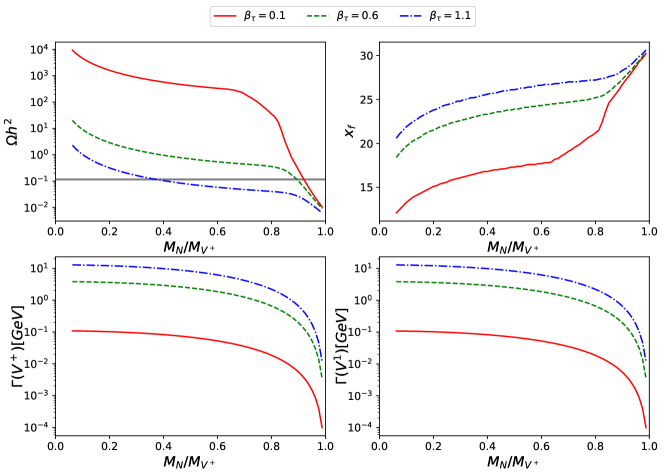
Figure 1: Relevant observables related with the early universe dynamics as a function of $M_{N}/M_{V}^{+}$ and different values of $\beta_{\tau}$. For these plots, we considered $M_{V^{+}}=800$[GeV] and $\beta_{e}=\beta_{\mu}=0$. The solid horizontal gray line in the first panel shows the measured value by PLANCK.

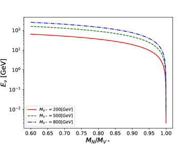
Figure 2: Energy of the non thermal relic neutrinos arising from the vector decay, as a function of $M_{N}/M_{V^{+}}$.

IV Relic density

In this section we generalize the results from the previous section considering different values for $\beta_{e}$ and $\beta_{\mu}$. We have performed a scan over the parameter space and computed the DM relic density. We constrained the parameter space considering the PLANCK measurement PLANCK which are reported as $\Omega h^{2}=0.1184\pm 0.0012$. As can be seen in Figure 3, the relic density is inversely proportional to the square sum of the couplings, presenting a strong suppression. This behavior can be used to define lower limits on the couplings for a given choice of $M_{N}$ and $M_{V^{+}}$. However, this is not possible when $M_{V^{+}}\geq 0.8M_{N}$, because in this case the thermal relic density is dominated by the vectors, and therefore the $\beta$ couplings don’t play a relevant role. We made a focus on the region of the parameter space satisfying $0.11\leq\Omega h^{2}\leq 0.12$, where the model can saturate the relic density up to $3\sigma$. This region can be seen in Figure 4, and it’s easier to note the change in channel contribution for $M_{V^{+}}\geq 0.8M_{N}$. It’s worth mentioning how the saturation region differs from the approximated results in our previous work colliderLHNL , a detailed discussion about this discrepancy can be found in X.

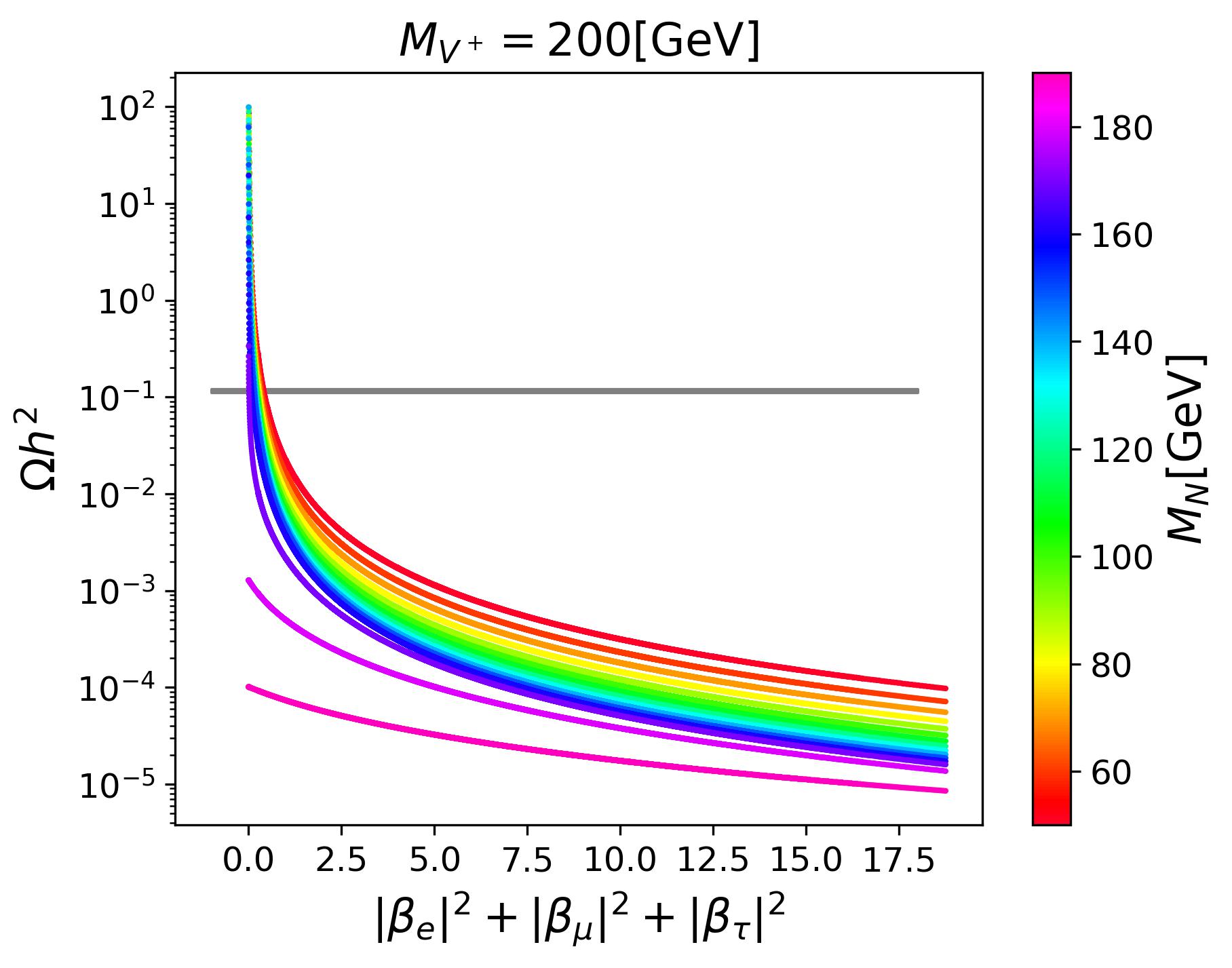
(a)

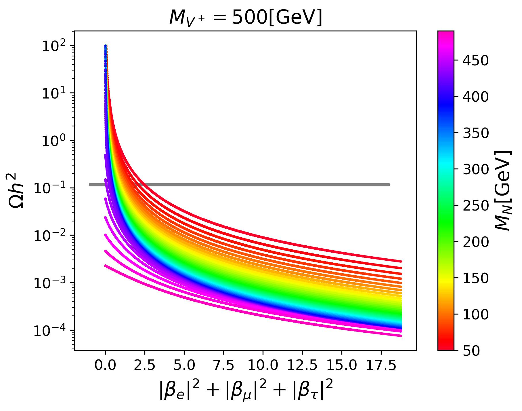
(b)

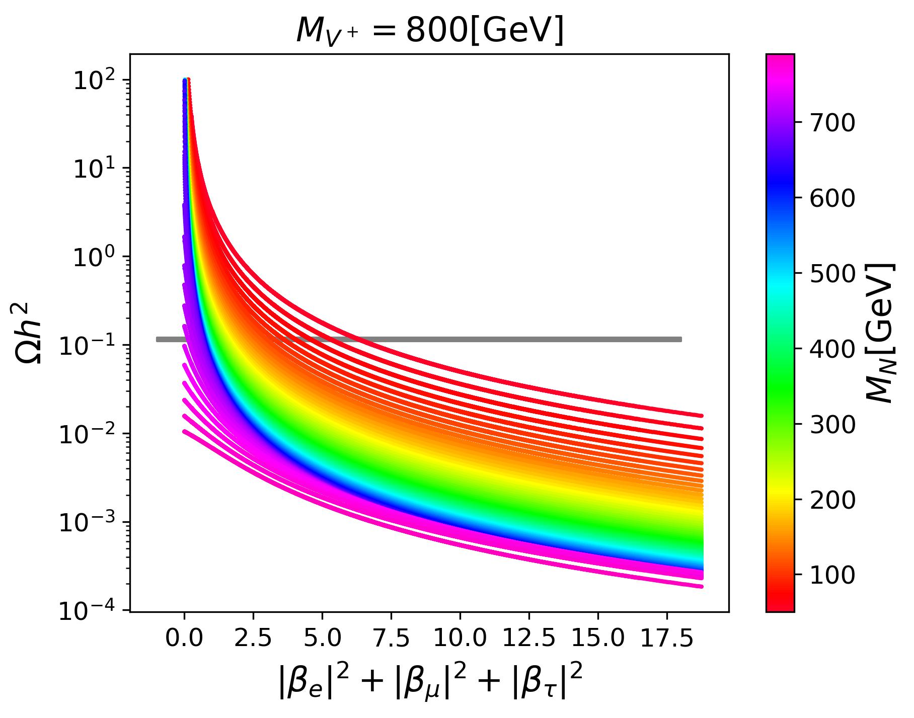
(c)

Figure 3: Relic density dependence on the squared sum of the $\beta$ couplings for different values of $M_{N}$ and $M_{V^{+}}$.

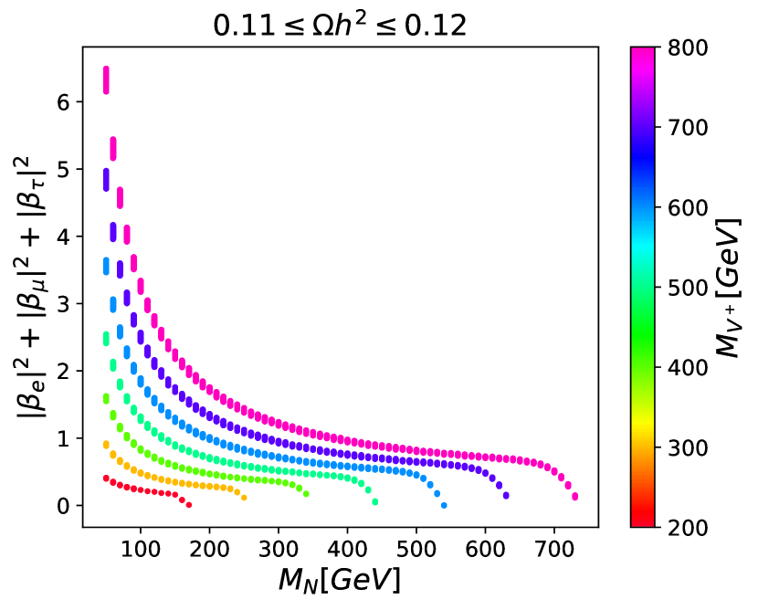
(a)

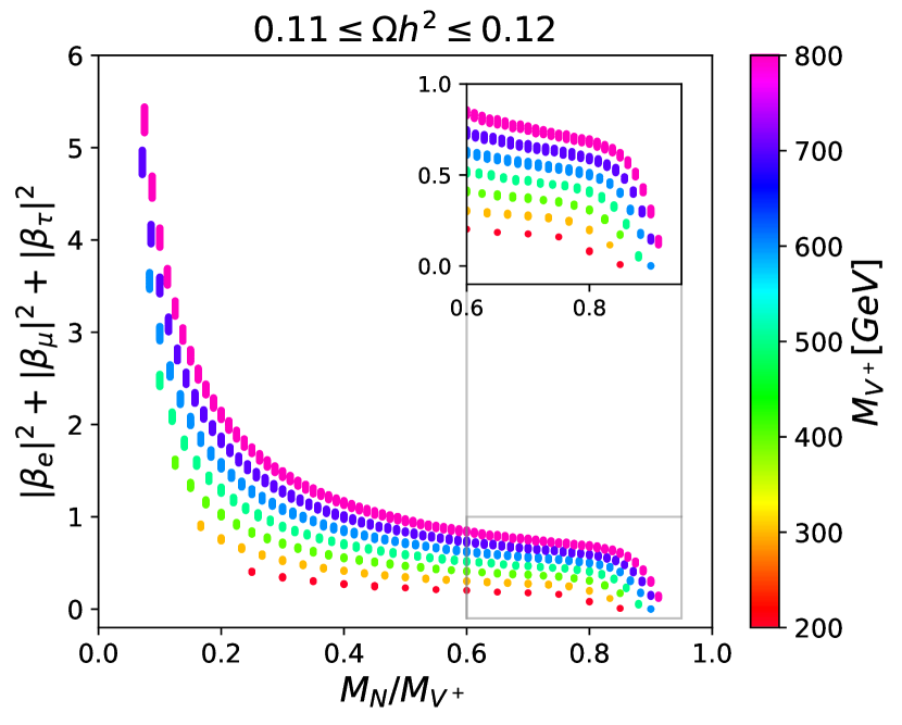
(b)

Figure 4: Parameter space points that saturate the dark matter relic abundance.

V Lepton Flavor Violation

While the DM relic abundance depends on the squared sum of the couplings, these are constrained by lepton flavor violation (LFV) decays. This type of process is very rare and the upper bound on these quantities can be seen in Table 2. According to Ref. ilakovac the branching fraction for charged LFV decay has the following form:

$$\text{Br}(l_{i}\to l_{j}\gamma)_{\kappa=-1}=\frac{|\beta_{i}|^{2}|\beta_{j}|^{2}g_{w}^{2}s_{w}^{2}m_{i}^{5}}{64(4\pi)^{4}M_{V^{+}}^{4}\Gamma_{i}}|G\left(M_{N}^{2}/M_{V^{+}}^{2}\right)|^{2},$$ (7)

with

$$G(x)=-\frac{2x^{3}+5x^{2}-x}{4(1-x)^{3}}-\frac{3x^{3}}{2(1-x)^{4}}\ln x.$$ (8)

This expression can be used to define limits on the product of couplings, for instance limits over $|\beta_{e}||\beta_{\mu}|$ as is shown in Figure 5. It’s worth mentioning that these limits are valid only when $\kappa=-1$, a different value for this parameter should affect the $G(x)$ function. Under this parameter setting, the $V^{+}$ magnetic moment has the same form as the $W^{+}$ magnetic moment, allowing us to use the results from Ref. ilakovac . This similarity could be relevant for UV completions of the model considering a larger gauge group.

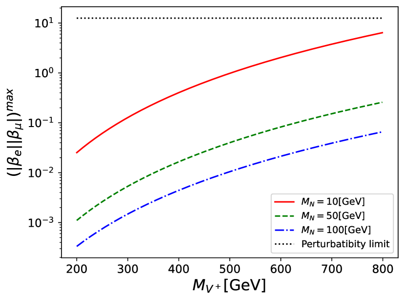
(a)

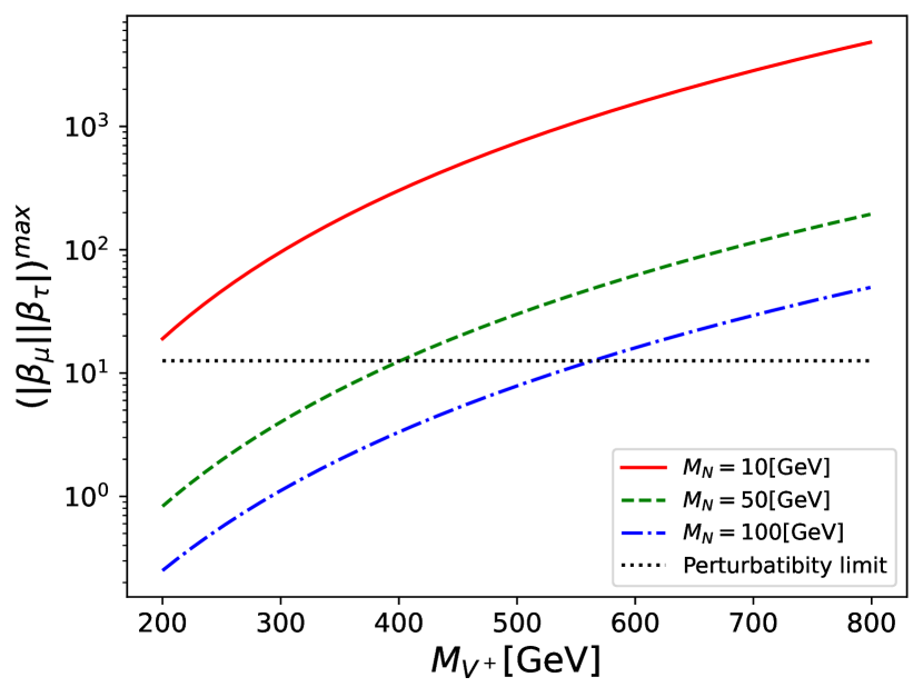
(b)

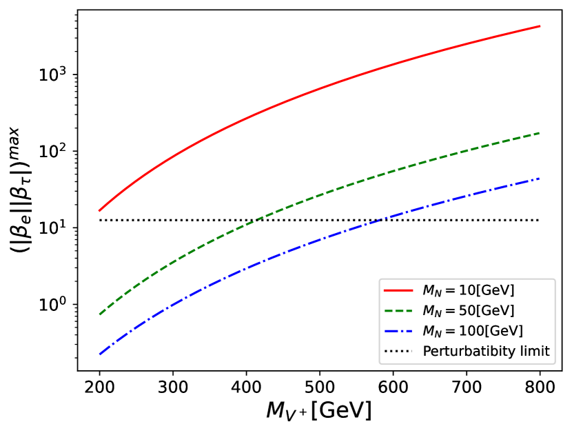
(c)

Figure 5: Upper limits for the product $|\beta_{i}||\beta_{j}|$ ($i,j=e,\mu,\tau$) for some reference values of $M_{N}$ and $M_{V^{+}}$. We notice that limits are relaxed for higher values of $M_{V^{+}}$.

process	branching fraction upper limit
$\mu\to e\gamma$	$<4.2\times 10^{-13}$
$\tau\to e\gamma$	$<3.3\times 10^{-8}$
$\tau\to\mu\gamma$	$<4.2\times 10^{-8}$

Table 2: Current limits on charged LFV decays, taken from Ref. pdg2022 .

In order to find points in the parameter space that satisfy both DM and LFV constraint, we implemented a Log-Likelihood function:

$$\ln\mathcal{L}=\ln\mathcal{L}^{DM}+\ln\mathcal{L}^{\mu\to e\gamma}+\ln\mathcal{L}^{\tau\to\mu\gamma}+\ln\mathcal{L}^{\tau\to e\gamma},$$ (9)

where all the likelihood functions are Gaussian. For the dark matter, we have centered the Gaussian on the Planck measurement for relic abundance, and we have set the standard deviation equal to the experimental uncertainty. For the LFV constraint, we have considered Gaussian likelihoods centered at 0 with a standard deviation equal to the upper bounds presented in Table 2 (in concordance with the method presented in Ref. scotosinglet ). Some representative likelihood profiles are shown in Figure 6. The scenario with $\beta_{e}\sim\beta_{\mu}\sim\beta_{\tau}$ is practically excluded, however, the maximum likelihood is obtained when the HNL couples to one lepton family only. The points satisfying $\beta_{i}=0$ and $\beta_{j}<<\beta_{k}$ are very close to the maximum likelihood for any combination of $i,j,k$

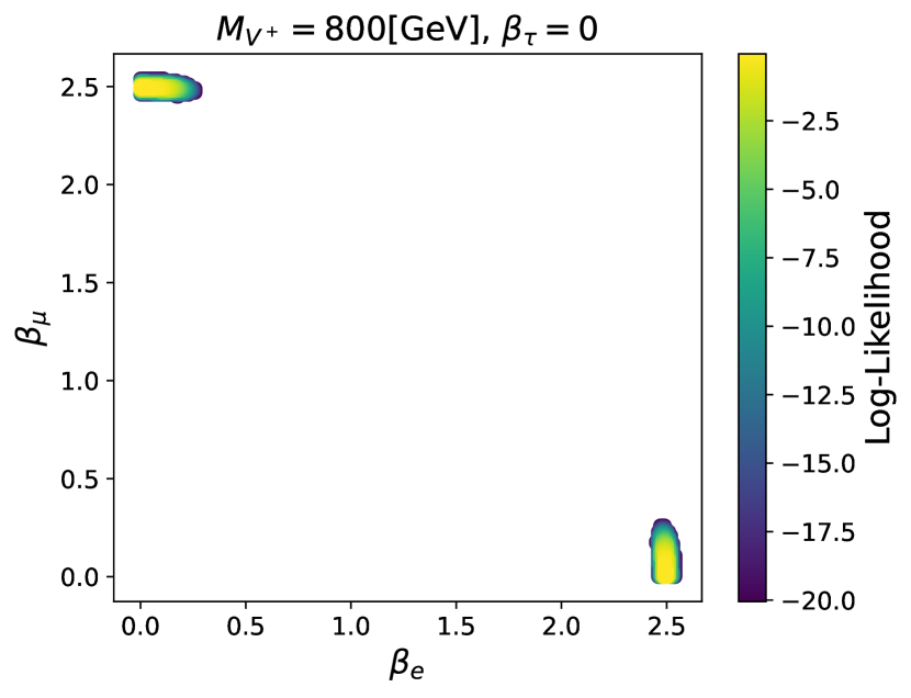
(a)

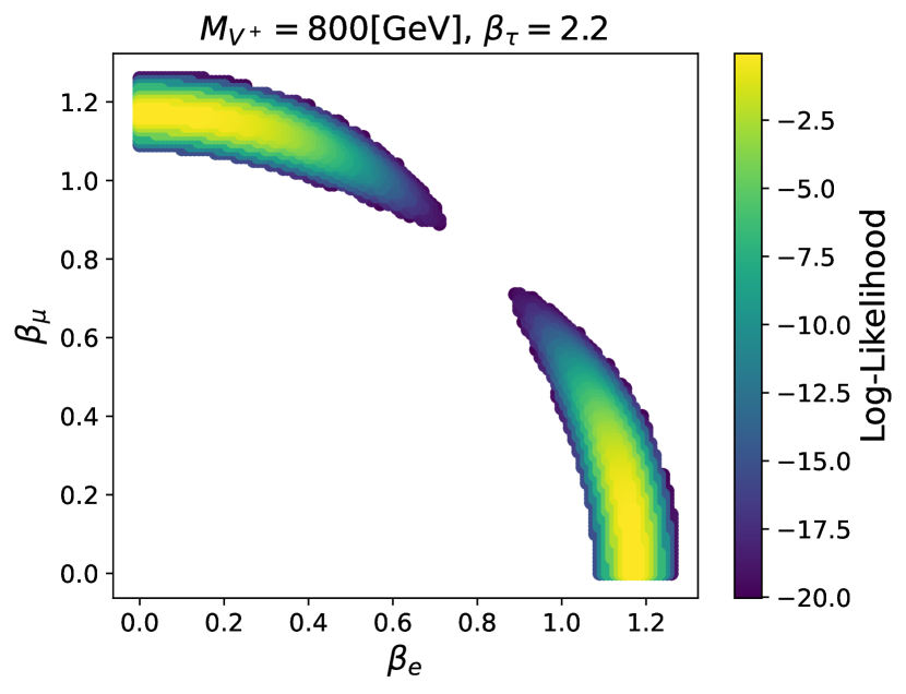
(b)

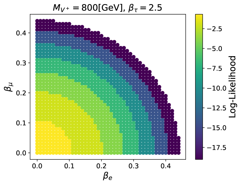
(c)

Figure 6: Log-Likelihood profiles for some special cases, considering $M_{N}=50$[GeV].

VI Indirect detection

The annihilation cross section into charged leptons has the following form:

$$\langle\sigma v\rangle(N_{L}N_{L}\to l^{+}l^{-})=\sqrt{1-\frac{m_{l}^{2}}{M_{N}^{2}}}\frac{m_{l}^{2}|\beta_{l}|^{4}(2M_{V^{+}}^{2}+M_{N}^{2}-m_{l}^{2})}{64\pi M_{V^{+}}^{4}(M_{V^{+}}^{2}+M_{N}^{2}-m_{l}^{2})}.$$ (10)

From Eq. 10, it can be seen that the most promising channel for indirect detection is $N_{L}N_{L}\to\tau^{+}\tau^{-}$ since $\langle\sigma v\rangle$ as a manifestation of helicity suppression. Therefore, we have studied this signal considering the exclusion limits from the Fermi-LAT telescope fermilims . On the other hand, the expected sensitivity of CTA ctalims could reach the threshold for observing this process. It’s worth mentioning that these limits were obtained by assuming that DM relic density is saturated by a single type of particle, therefore we defined $\mathcal{F}=\frac{\Omega h^{2}}{0.12}$ as a weight for underabundant parameter space points. Since annihilation implies the interaction between two dark matter particles, the annihilation cross section must be weighted as $\mathcal{F}^{2}\langle\sigma v\rangle$. The result can is shown in Figure 7. In general, the model prediction is much lower than the expected sensitivity of CTA, making the model hard to probe in the near future by means of CTA. However, there is a small region of the parameter space for low values of $M_{N}$ and $M_{V^{+}}$ that is excluded by Fermi-LAT,

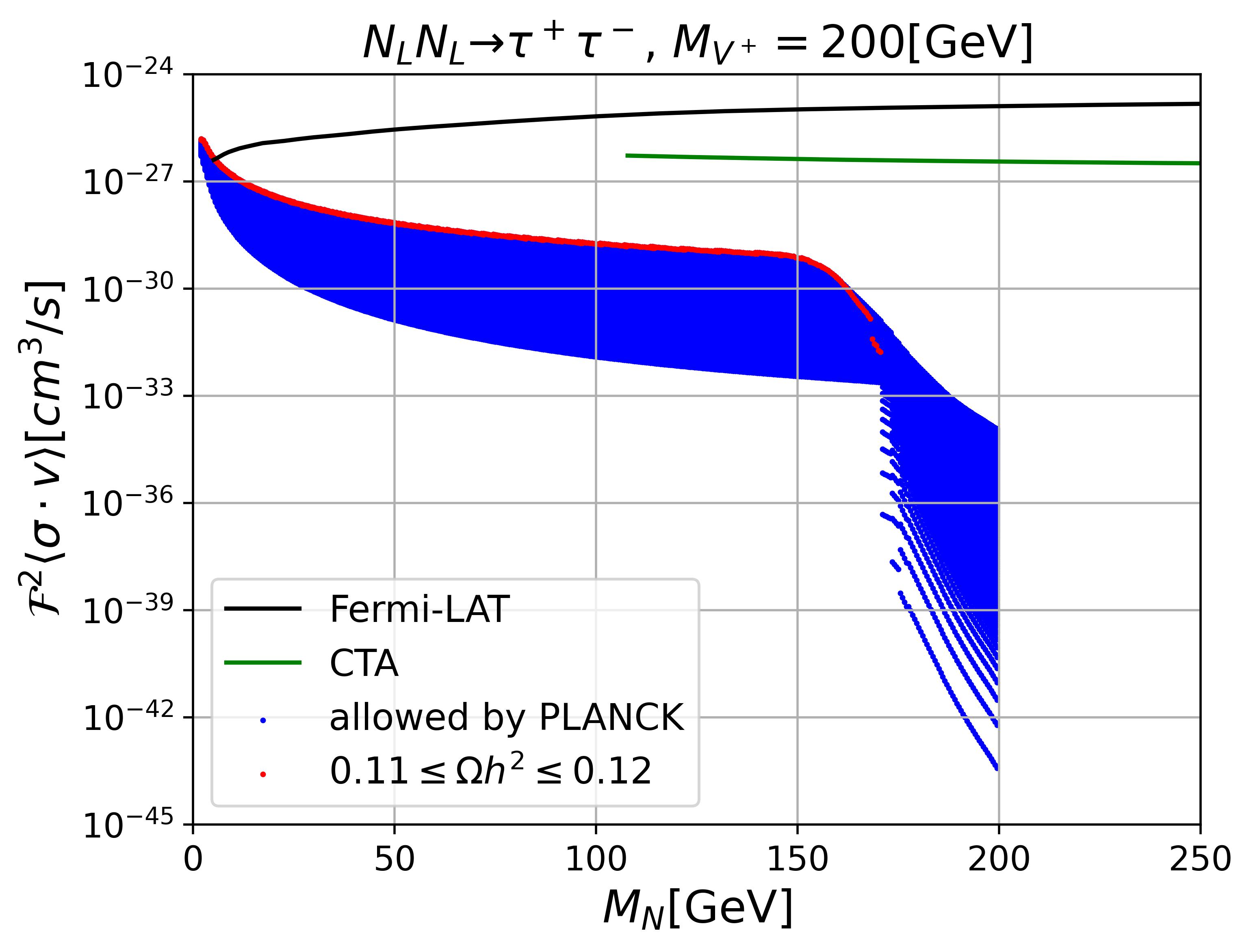
(a)

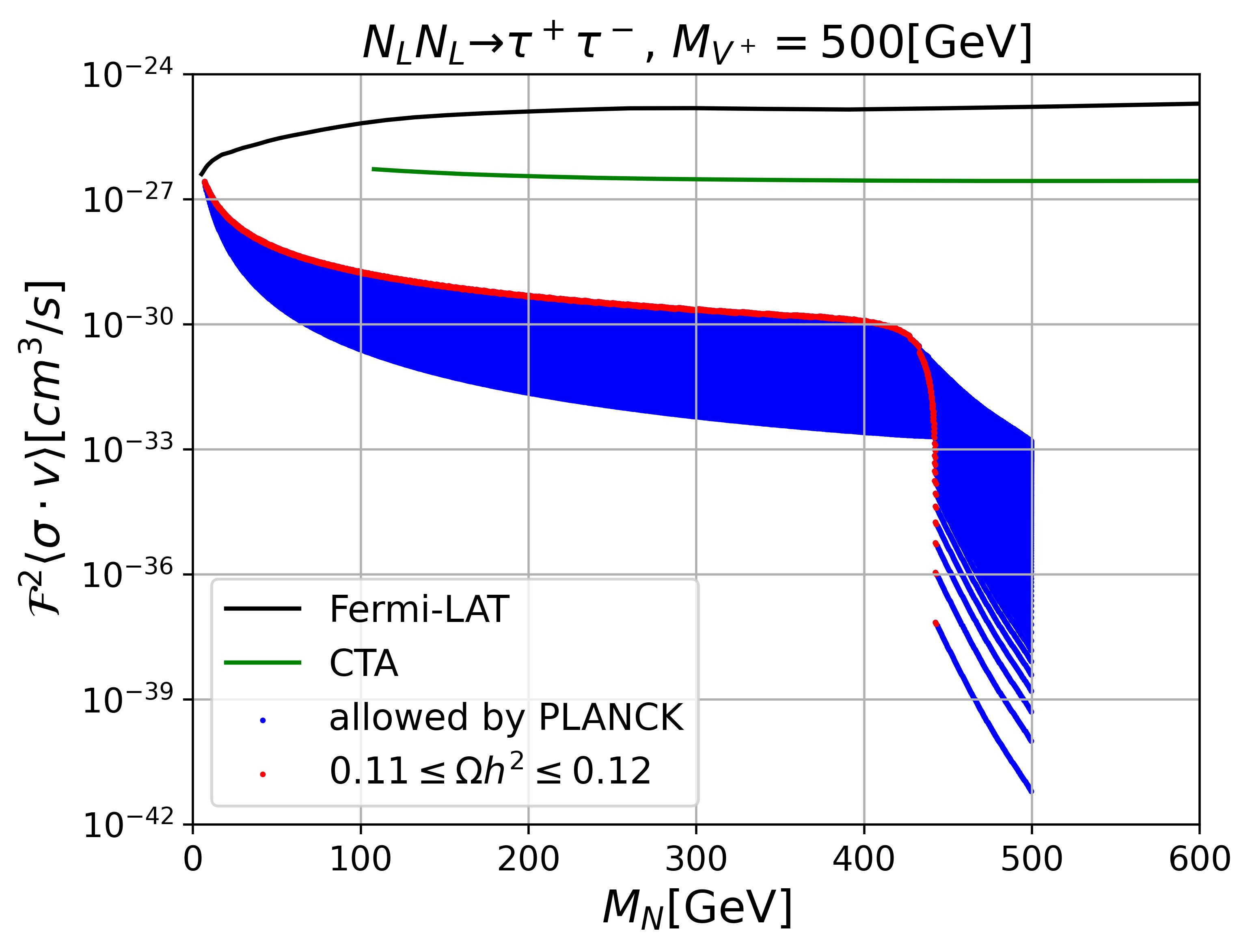
(b)

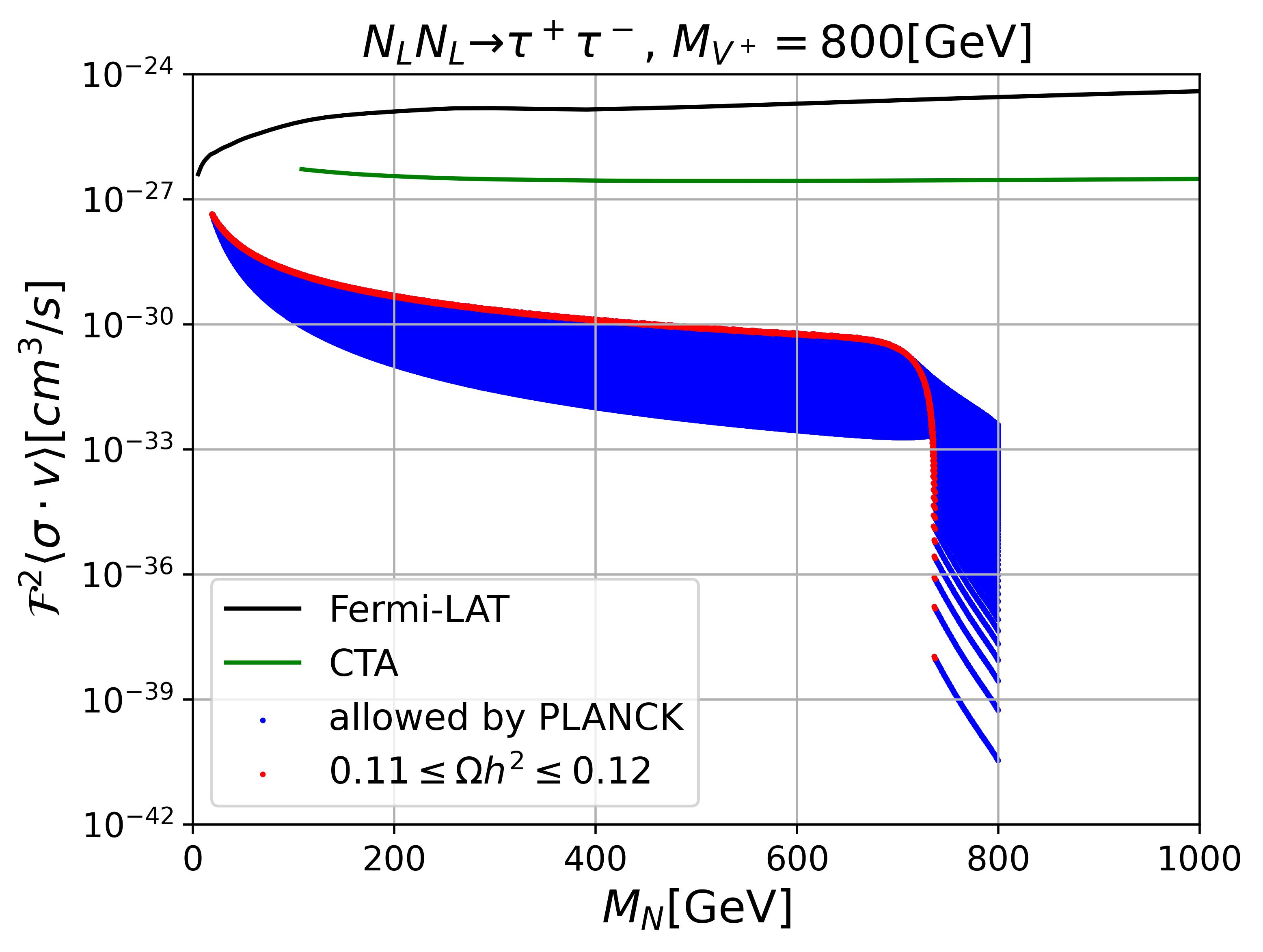
(c)

Figure 7: Model prediction for indirect detection. It’s worth recalling that these plots were obtained considering $\beta_{e}=\beta_{\mu}=0$. This choice gives the most optimistic prediction because higher values for these parameters would reduce the weighting factor.

VII Detectability at the LHC

In a previous work, we demonstrated that the production of 2 left HNLs can produce a distinctive signal at the LHC colliderLHNL , which is composed by a same flavor opposite sign lepton pair and missing energy. In that work, we fixed $\kappa=1$, therefore we computed the cross section of the process $pp\to N_{L}N_{L}\mu^{+}\mu^{-}$ for some benchmark points and $\kappa=1,-1$, as can be seen in Table 3. Firstly, we can note that the cross sections are slightly higher for $\kappa=-1$ for all benchmark points. On the other hand, we notice that the scenario where $\beta_{\mu}>>\beta_{e},\beta_{\tau}$ predicts cross sections that are inconsistent with the ATLAS upper limits susylims_dy , therefore this scenario is disregarded. Finally, the scenario where $\beta_{\tau}>>\beta_{e},\beta_{\mu}$ predicts smaller cross sections due to the decay width suppression, making this scenario more promising, predicting small cross sections at colliders and the highest possible indirect detection rate.

$M_{V^{+}}$[GeV]	$\beta_{e}$	$\beta_{\mu}$	$\beta_{\tau}$	$\sigma_{\kappa=1}$[fb]	$\sigma_{\kappa=-1}$[fb]
$200$	$0.00$	$0.06$	$0.63$	$6.98\times 10^{-5}$	$1.29\times 10^{-4}$
$200$	$0.00$	$0.64$	$0.00$	$1.1\times 10^{3}$	$2\times 10^{3}$
$500$	$0.00$	$0.01$	$1.56$	$1.47\times 10^{-7}$	$4.21\times 10^{-8}$
$500$	$0.00$	$1.56$	$0.00$	$8.7$	$24.9$
$800$	$0.00$	$0.06$	$2.49$	$1.56\times 10^{-7}$	$5.71\times 10^{-7}$
$800$	$0.00$	$2.5$	$0.00$	$0.47$	$1.7$

Table 3: Benchmark points that saturate relic density and the production cross section for different values of $\kappa$.

For the sake of completeness, we computed the production cross section for different parameter space points, relating this value with the predicted relic density. For this sample, we have obtained the effective cross section, $\sigma_{eff}$ following the methodology presented in our previous work colliderLHNL (note that, since we are interested in HL-LHC projections, we are keeping the most optimistic value of $\epsilon=0.55$ for the detector efficiency). As can be seen in Figure 8, there is an inverse relation between these two variables, and the $\beta_{\tau}$ parameter plays a key role in this correlation. Additionally, we included the expected sensitivities $Z^{HL}$ for the HL-LHC at $3000[\text{fb}^{-1}]$, showing that the model can account for a significant fraction of the dark matter relic abundance and be probed at the HL-LHC.

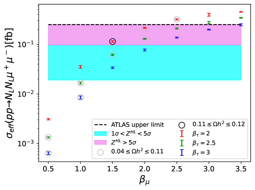
(a)

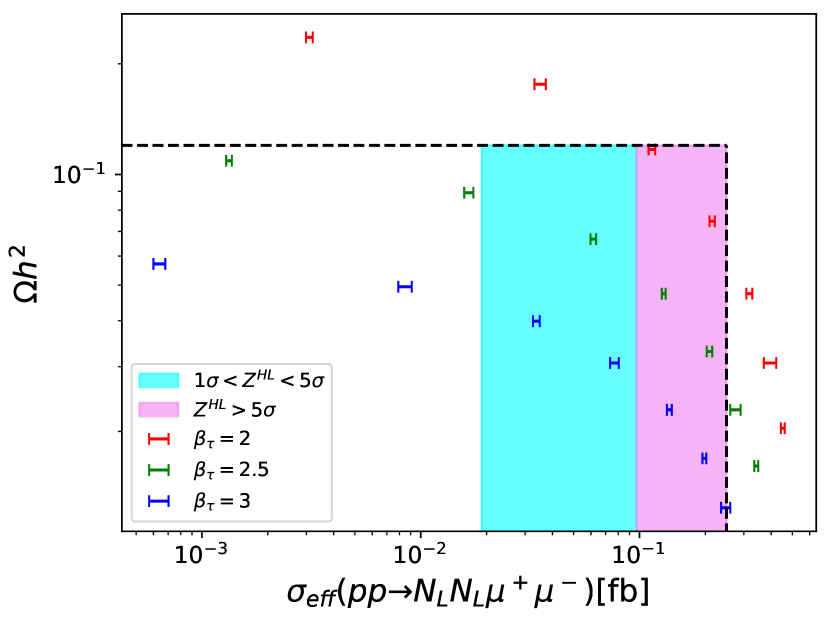
(b)

Figure 8: Correlations between the production cross section and relic density, for $\beta_{e}=0,\kappa=-1,M_{V^{+}}=800\text{[GeV]},M_{N}=50\text{[GeV]}$ and different values for $\beta_{\mu}$. The dashed lines represent the exclusion limits in both observables.

It’s worth mentioning that these results are valid in the region where the vectors are prompt particles. In the nearly degenerate regime, the couplings can be arbitrarily small and escape the DM constraint, allowing the vector to be a long lived particle, as depicted in Figure 9. However, the resulting lepton from the vector decay would be soft due to the small mass splitting, in concordance with the discussion about early universe neutrinos presented in Section III. However, depending on the vector’s lifetime, a region of the parameter space could be probed in the context of long living particles. For instance, if we consider the CMS searches of displaced muons CMS-PAS-EXO-14-012 , displaced muons with $p_{T}>26$[GeV] can be reconstructed at CMS (there are additional cuts for the definition of the acceptance region, but for the sake of a general discussion we will consider only this cut). The energy of the displaced muon depends only on the kinematics and therefore on the mass splitting. While the mass splitting is small, a region of the parameter space can be probed under this setup, as can be seen in Figure 10.

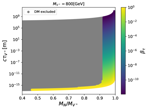
Figure 9: Decay length as a function of $M_{N}/M_{V^{+}}$. For this plot, we considered $\beta_{e}=\beta_{\mu}=0$.

Figure 10: Region of the parameter space that can be probed in the context of LLPs for different cuts. These limits are derived from neglecting the muon mass.

VIII Conclusions

In this work, we studied the dark matter phenomenology of the Vector Scotogenic Model, composed by a massive vector doublet under $SU(2)_{L}$ and a left-handed Heavy Neutral Lepton. We focused in the scenario where the HNL is the dark matter candidate. We separated the parameter space in two regions, separated by the mass split between the HNL and the new vector states. When the fermion mass is not comparable to the vector mass, the early universe dynamics is dominated by fermion annihilation, and it is possible to define lower bounds on the couplings between the new fields and the SM leptons. When the mass split is small enough, the vectors are thermally produced and their annihilation becomes relevant, contributing to the relic density even when the above mentioned couplings are small. The thermal production of the vector states generates strong consequences related to the non thermal production of relic neutrinos, and this effect should be studied in depth. On the other side, both regimes can be probed at colliders, the first one with prompt searches and the second one under the paradigm of long living particles. Besides that, the annihilation cross section is too small to be probed in the context of indirect detection, therefore collider experiments are the most promising way to probe this model.

Aknowledgements

This work was funded by ANID - Millennium Program - ICN2019_044. Also, we would like to thank to the DGIIP-UTFSM for funding during the development of this work. AZ was partially supported by Proyecto ANID PIA/APOYO AFB220004 (Chile) and Fondecyt 1230110.

IX Appendix A: Contribution of annihilation channels

The early universe dynamics is governed by three processes types of processes: $NN\to ll$, $NV\to SM\quad SM$ and $VV\to SM\quad SM$. The annihilation cross section has the following dependence:

$$\langle\sigma\cdot v\rangle=|\beta|^{4}F^{NN}+|\beta|^{2}(g_{w}^{2}+\lambda_{L}^{2})F^{NV}+(\lambda_{L}^{2}+g_{w}^{2})^{2}F^{VV}$$ (11)

When $|\beta|\to 0$ and $M_{N}<<M_{V^{+}}$, the cross section is dominated by $F^{VV}$. However, since the vectors are heavier, they decouple before the freeze out, producing overabundance. When the masses are similar, vector decoupling occurs near the actual freeze-out, avoiding overabundance even when the fermion channel is suppressed. All these conclusions are obtained and validated by the results in Table 4

$M_{N}/M_{V^{+}}$	$\beta_{\tau}$	$\%NN$	$\%VN$	$\%VV$	$\Omega h^{2}$
0.625	0.01	0	100	0	$3.24\times 10^{4}$
0.625	0.90	100	0	0	$0.115$
0.75	0.01	0	100	0	$2.77\times 10^{3}$
0.75	0.90	100	0	0	$9.19\times 10^{-2}$
0.9375	0.01	0	0	100	$5.88\times 10^{-2}$
0.9375	0.90	16	$44-55$	$29-40$	$2.21\times 10^{-2}$

Table 4: Relic density for some reference values, with the contributions of each channel. This table was obtained with $M_{V^{+}}=800$[GeV], and the uncertainty in the last row comes from the several channels contributing less than $1\%$.

X Appendix B: Comparison of the complete and approximated calculation of relic density

In our previous work, we used the results from Ref. dong2021 to set lower limits on the parameter space, using the following expression:

$$\langle\sigma v\rangle^{0}=\sum_{k,k^{\prime}=\{e,\mu,\tau\}}|\beta_{k}^{*}\beta_{k^{\prime}}|^{2}\frac{M_{N}^{2}}{8\pi}\left(1+\frac{8T_{f}}{M_{N}}\right)\left(\frac{1}{M_{V^{+}}^{4}}+\frac{4}{(M_{V^{1}}^{2}+M_{V^{2}}^{2})^{2}}\right).$$ (12)

In order to avoid over abundance, this expression must satisfy $\langle\sigma v\rangle^{0}\geq 3\times 10^{-9}[GeV^{-2}]$. This constraint is a rough estimation, and therefore we decided to compare our present results with this expression. As can be seen in Figure 11, our current results present a stronger constraint on the parameter space. However, taking a more stringent limit of $\langle\sigma v\rangle^{0}\geq 3\times 10^{-8}[GeV^{-2}]$ gives closer results to the micrOMEGAs calculation. On the other hand, Eq. (12) doesn’t account for co-annihilations, therefore it fits well the region where $M_{N}<<M_{V^{+}}$, but it doesn’t describe well the nearly degenerate regime.

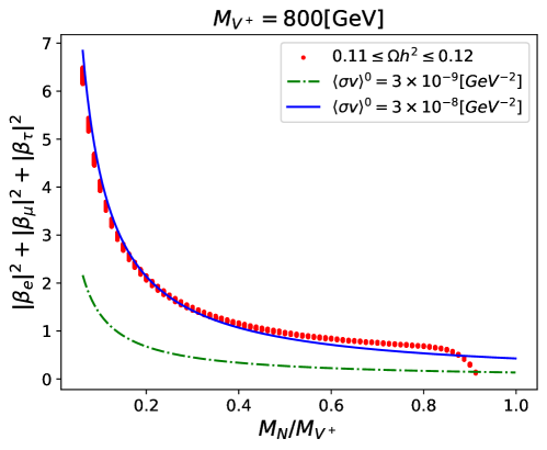
Figure 11: Comparison between the rough approximation considered in our previous work and the relic density computation with micrOMEGAs.

References

- (1) Planck Collaboration, P. A. R. Ade et al., “Planck 2015 results. XIII. Cosmological parameters,” Astron. Astrophys. 594 (2016) A13, arXiv:1502.01589 [astro-ph.CO].
- (2) E. Ma, “Verifiable radiative seesaw mechanism of neutrino mass and dark matter,” Phys. Rev. D 73 (2006) 077301, arXiv:hep-ph/0601225.
- (3) A. E. Cárcamo Hernández, J. Vignatti, and A. Zerwekh, “Generating lepton masses and mixings with a heavy vector doublet,” J. Phys. G 46 no. 11, (2019) 115007, arXiv:1807.05321 [hep-ph].
- (4) P. Van Dong, D. Van Loi, L. D. Thien, and P. N. Thu, “Novel imprint of a vector doublet,” Phys. Rev. D 104 no. 3, (2021) 035001, arXiv:2104.12160 [hep-ph].
- (5) P. A. C., J. Zamora-Saa, and A. R. Zerwekh, “Probing left-handed heavy neutral leptons in the Vector Scotogenic Model,” JHEP 02 (2024) 153, arXiv:2211.09753 [hep-ph].
- (6) B. D. Sáez, F. Rojas-Abatte, and A. R. Zerwekh, “Dark Matter from a Vector Field in the Fundamental Representation of ,” Phys. Rev. D 99 no. 7, (2019) 075026, arXiv:1810.06375 [hep-ph].
- (7) G. Belanger, F. Boudjema, A. Pukhov, and A. Semenov, “micrOMEGAs3: A program for calculating dark matter observables,” Comput. Phys. Commun. 185 (2014) 960–985, arXiv:1305.0237 [hep-ph].
- (8) G. Belanger, F. Boudjema, A. Pukhov, and A. Semenov, “MicrOMEGAs 2.0: A Program to calculate the relic density of dark matter in a generic model,” Comput. Phys. Commun. 176 (2007) 367–382, arXiv:hep-ph/0607059.
- (9) C. Hagedorn, J. Herrero-García, E. Molinaro, and M. A. Schmidt, “Phenomenology of the Generalised Scotogenic Model with Fermionic Dark Matter,” JHEP 11 (2018) 103, arXiv:1804.04117 [hep-ph].
- (10) S. Baumholzer, V. Brdar, P. Schwaller, and A. Segner, “Shining Light on the Scotogenic Model: Interplay of Colliders and Cosmology,” JHEP 09 (2020) 136, arXiv:1912.08215 [hep-ph].
- (11) Y. Du, F. Huang, H.-L. Li, Y.-Z. Li, and J.-H. Yu, “Revisiting dark matter freeze-in and freeze-out through phase-space distribution,” JCAP 04 no. 04, (2022) 012, arXiv:2111.01267 [hep-ph].
- (12) J. S. Alcaniz, J. P. Neto, F. S. Queiroz, D. R. da Silva, and R. Silva, “The Hubble constant troubled by dark matter in non-standard cosmologies,” Sci. Rep. 12 no. 1, (2022) 20113, arXiv:2211.14345 [astro-ph.CO]. [Erratum: Sci.Rep. 13, 209 (2023)].
- (13) A. Ilakovac and A. Pilaftsis, “Flavor violating charged lepton decays in seesaw-type models,” Nucl. Phys. B 437 (1995) 491, arXiv:hep-ph/9403398.
- (14) Particle Data Group Collaboration, R. L. Workman et al., “Review of Particle Physics,” PTEP 2022 (2022) 083C01.
- (15) A. Beniwal, J. Herrero-García, N. Leerdam, M. White, and A. G. Williams, “The ScotoSinglet Model: a scalar singlet extension of the Scotogenic Model,” JHEP 21 (2020) 136, arXiv:2010.05937 [hep-ph].
- (16) M. Di Mauro, M. Stref, and F. Calore, “Investigating the effect of Milky Way dwarf spheroidal galaxies extension on dark matter searches with Fermi-LAT data,” Phys. Rev. D 106 no. 12, (2022) 123032, arXiv:2212.06850 [astro-ph.HE].
- (17) CTA Collaboration, A. Acharyya et al., “Sensitivity of the Cherenkov Telescope Array to a dark matter signal from the Galactic centre,” JCAP 01 (2021) 057, arXiv:2007.16129 [astro-ph.HE].
- (18) ATLAS Collaboration, G. Aad et al., “Search for electroweak production of charginos and sleptons decaying into final states with two leptons and missing transverse momentum in TeV collisions using the ATLAS detector,” Eur. Phys. J. C 80 no. 2, (2020) 123, arXiv:1908.08215 [hep-ex].
- (19) CMS Collaboration, “Search for long-lived particles that decay into final states containing two muons, reconstructed using only the CMS muon chambers,” tech. rep., CERN, Geneva, 2015. http://cds.cern.ch/record/2005761.