RISnet: A Domain-Knowledge Driven Neural Network Architecture for RIS Optimization with Mutual Coupling and Partial CSI

Abstract

Multiple access (MA) techniques are cornerstones of wireless communications. Their performance depends on the channel properties, which can be improved by reconfigurable intelligent surfaces (RISs). In this work, we jointly optimize MA precoding at the base station (BS) and RIS configuration. We tackle difficulties of mutual coupling between RIS elements, scalability to more than 1000 RIS elements, and channel estimation. We first derive an RIS-assisted channel model considering mutual coupling, then propose an unsupervised machine learning (ML) approach to optimize the RIS. In particular, we design a dedicated neural network (NN) architecture RISnet with good scalability and desired symmetry. Moreover, we combine ML-enabled RIS configuration and analytical precoding at BS since there exist analytical precoding schemes. Furthermore, we propose another variant of RISnet, which requires the channel state information (CSI) of a small portion of RIS elements (in this work, 16 out of 1296 elements) if the channel comprises a few specular propagation paths. More generally, this work is an early contribution to combine ML technique and domain knowledge in communication for NN architecture design. Compared to generic ML, the problem-specific ML can achieve higher performance, lower complexity and symmetry.

I Introduction

The multiple access (MA) techniques (e.g., space-division multiple access (SDMA) and non-orthogonal multiple access (NOMA)) are cornerstones of multi-user wireless communications. Their performance depends heavily on the channel condition. For example, a high channel gain realizes a high signal-to-noise ratio (SNR), a high-rank multiple-input-multiple-output (MIMO) channel matrix makes it possible to serve multiple users via SDMA [3] and a degraded [4] or quasi-degraded channel [5] is beneficial for the NOMA performance. In recent years, the reconfigurable intelligent surface (RIS) [6] is proposed to manipulate the channel property and enhance the MA performance. In this paper, we consider the problem of joint optimization of precoding at the base station (BS) and configuration of the RIS for SDMA and NOMA.

In the literature, multiple precoding techniques have been proposed for SDMA at the BS, including maximum ratio transmission (MRT), zero-forcing (ZF), minimum mean square error (MMSE) precoding [7], and the weighted minimum mean square error (WMMSE) precoding with proved equivalence to weighted sum-rate (WSR) maximization [8]. The optimality of NOMA in degraded channels is demonstrated in [4]. An optimal NOMA precoding scheme for a multi-antenna BS in a quasi-degraded channel is derived in [5, 9]. The joint optimization of precoding and RIS configuration is performed with block coordinate descent (BCD) [10], majorization-minimization (MM) [11, 12] and alternating direction method of multipliers (ADMM) [13] algorithms to maximize the WSR in SDMA. The RIS is also applied to make a channel quasi-degraded and minimize the transmit power subject to the required rate using successive convex approximation (SCA) [14] and semidefinite relaxation (SDR) [15, 16] algorithms. In addition, Riemannian manifold conjugate gradient (RMCG) and Lagrangian method are applied to optimize multiple RISs and BSs to serve cell-edge users [17]. The impact of RISs on the outage probability in NOMA is studied [18]. Successive refinement algorithm and exhaustive search are applied for passive beamforming improvement [19]. The active RISs is optimized with the SCA algorithm to maximize the SNR [20]. The gradient-based optimization is applied to optimize the effective rank and the minimum singular value [21].

In general, the above analytical iterative methods do not scale well with the number of RIS elements. No more than 100 elements are assumed in [10, 11, 13, 17, 19, 12, 18, 20, 14, 15, 16] and up to 400 RIS elements are assumed in [21], which is far from the vision of more than 1000 RIS elements [22] and the requirement in many scenarios to realize a necessary link budget [23]. Another common important limitation of the analytical optimization approaches is that suboptimal approximations are applied to make the problem solvable [10, 19, 13, 14]. Moreover, the required numbers of iterations make the proposed iterative algorithms difficult to be implemented in real time since the computation time is longer than the channel coherence time.

A noticeable effort is to apply machine learning (ML) to optimize the RIS, which bypasses the difficulty of analytical solution via the universal approximation property of the neural network (NN) [24]. Recently, deep learning (DL) and reinforcement learning (RL) are applied and compared for RIS optimization [25]. Long short-term memory (LSTM) and deep Q-network (DQN) are applied to optimize RIS for NOMA [26]. The simultaneously transmitting and reflecting (STAR)-RIS is combined with NOMA [27]. RL is applied to maximize the sum-rate in SDMA [28], and NOMA [29, 28] and energy efficiency in NOMA [30]. The achievable rate is predicted and the RIS is configured with DL [31]. The RIS is configured directly with received pilot signals [32]. The mapping from received pilot signal to the phase shifts is optimized [33]. Due to the separation of training and testing phases, the trained ML model is able to be applied in real time. However, the scalability with the number of RIS elements is still limited [26, 29, 16, 28, 32, 33].

Another common limitation of many works on RIS is the full channel state information (CSI) assumption (e.g., [10, 12, 13, 19, 20]). Due to the large number of elements, the full CSI of all elements is very difficult to obtain in real time. Possible countermeasures are, e.g., codebook-based RIS optimization [23, 34]. However, the beam training is still a major limitation.

A third common limitation of many works is the assumption of perfect RIS without mutual coupling. Due to the small distance between two adjacent elements, it is highly likely that there exists certain mutual coupling in the RIS. In the literature, a single-input single-output (SISO) RIS-assisted system is optimized [35]. A mutual impedance-based communication model considering mutual coupling is presented [36]. A mutual coupling aware characterization and performance analysis of the RIS is introduced [37]. The RIS architecture is modeled and characterized using scattering parameter network analysis [38]. A closed-form expression of RIS-assisted MIMO channel model in a general sense, i.e., considering RIS mutual coupling, with the direct channel from BS to users and without the unilateral approximation [39], is still an open problem.

Summarizing the state-of-the-art, we identify three limitations of current RIS research: the insufficient consideration of mutual coupling, the poor scalability to consider more than 1000 RIS elements and the unrealistic assumption of full CSI.

In this work, we propose a dedicated NN architecture RISnet and an unsupervised ML approach to address these limitations. Our contribution is four-fold as follows.

• We derive an RIS channel model considering the mutual coupling between RIS elements. The derivation is based on the scattering parameter network analysis [38]. A closed-form expression is derived without unilateral approximation.

• We propose an NN architecture RISnet for RIS configuration. The number of RISnet parameters is independent from the number of RIS elements, enabling a high scalability. Furthermore, a permutation-invariant RISnet is proposed for SDMA, where any permutation of users in the input has no impact on the RIS phase shifts because permutation of users has no impact on the SDMA problem. Another variant of RISnet is permutation-variant for NOMA, reflecting the importance of decoding order in NOMA.

• The CSI is extremely difficult to obtain due to the large number of RIS elements. We propose an improved RISnet, where only a few RIS elements (in our paper, 16 out of 1296) are equipped with RF chains and can estimate the channel with the pilot signals from users. We demonstrate that RISnet can configure the phase shifts of all RIS elements with the partial CSI of a few RIS elements if the channel is sparse. In this way, a good compromise between hardware complexity and performance is achieved.

• We combine ML-enabled RIS configuration and analytical precoding. For SDMA and NOMA, we develop different strategies to combine analytical precoding and ML: The WMMSE precoding for SDMA is iterative and not differentiable. Therefore, we use alternating optimization (AO). The precoding in quasi-degraded channels in NOMA has a differentiable form. Therefore, the precoding is part of the objective function.

We combine domain knowledge in communication and ML for NN architecture and training process design. It not only solves the RIS configuration problem, but can also inspire solutions to other problems. According to [40], incorporating domain knowledge is considered as one of the three grand challenges in ML. We show that an NN architecture tailored for the considered problem is superior in scalability, complexity, performance and robustness.

This work is based on our preliminary results [1, 2]. The preliminary work [1] assumes constant rate requirements and does not consider partial CSI. In this work, we significantly enhance flexibility and feasibility by including rate requirement in the input and using partial CSI. We also maximize the WSR in this work instead of sum-rate in [2], where the weights are input of the RISnet, significantly improving the flexibility to choose an operational point according to the requirement. Beyond them, we consider the mutual coupling between the RIS elements. Furthermore, we provide a comparison study between the permutation-invariant SDMA and the permutation-variant NOMA, proposing two variants of the RISnet according to this property. We also discuss possibilities to combine analytical precoding techniques with ML, depending on the differentiability of the analytical method.

Notations: $(\cdot)^{+}$ denotes the pseudo-inverse operation, $|a|$ and $\arg(a)$ are amplitude and phase of complex number $a$, respectively, $\mathbf{T}[\cdot,j,k]$ denotes the vector of the elements with position $(j,k)$ in the second and third dimensions in the three-dimensional tensor $\mathbf{T}$, $\mathbf{1}^{a\times a}$ is the matrix of all ones with shape $a\times a$, and $\mathbf{I}^{a\times a}$ is the identity matrix with shape $a\times a$, i.e., all diagonal elements of $\mathbf{I}^{a\times a}$ are ones, all off-diagonal elements are zeros. We also define $\mathbf{E}^{a\times a}=\mathbf{1}^{a\times a}-\mathbf{I}^{a\times a}$.

II The RIS Channel Model Considering Mutual Coupling

We consider an RIS-aided multi-user multiple-input-single-output (MISO) scenario, as depicted in Figure 1. The channel from BS to RIS is denoted as $\mathbf{H}\in\mathbb{C}^{N\times M}$, where $N$ is the number of RIS elements and $M$ is the number of BS antennas. The channel from RIS to users is denoted as $\mathbf{G}\in\mathbb{C}^{U\times N}$, where $U$ is the number of users. The channel from BS to users directly is denoted as $\mathbf{D}\in\mathbb{C}^{U\times M}$.

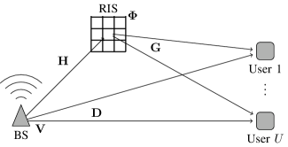
Figure 1: The system model of RIS-assisted downlink multi-user broadcasting.

Denote the precoding matrix as $\mathbf{V}\in\mathbb{C}^{M\times U}$ and the signal processing matrix of the RIS as the diagonal matrix $\bm{\Phi}\in\mathbb{C}^{N\times N}$, where the diagonal element in row $n$ and column $n$ is $\phi_{nn}=e^{j\psi_{n}}$, where $\psi_{n}\in[0,2\pi)$ is the phase shift of RIS element $n$. Conventionally, the channel $\mathbf{C}$ between BS and users is [10]

$$\mathbf{C}=\mathbf{D}+\mathbf{G}\bm{\Phi}\mathbf{H},$$ (1)

and the signal received at the users is

$$\mathbf{y}=\mathbf{C}\mathbf{V}\mathbf{x}+\mathbf{n},$$ (2)

where $\mathbf{x}\in\mathbb{C}^{U\times 1}$ is the transmitted symbols, $\mathbf{y}\in\mathbb{C}^{U\times 1}$ is the received symbols, and $\mathbf{n}\in\mathbb{C}^{U\times 1}$ is the noise.

An implicit assumption of (1) is that the RIS elements do not have mutual coupling with each other. Therefore, its signal processing can be described as a diagonal matrix $\bm{\Phi}$. However, it is likely that there exists mutual coupling between elements due to the small distance between each other. In the following, we assume transmitter and receiver without mutual coupling and an RIS with mutual coupling.

Our derivation is a generalization of Section III in [38]. We define the S-parameter matrix $\mathbf{S}$ for the signal transmission system shown in Figure 1 and partition it as

$$\mathbf{S}=\left[\begin{array}[]{ccc}\mathbf{S}_{TT}&\mathbf{S}_{TI}&\mathbf{S}_{TR}\\ \mathbf{S}_{IT}&\mathbf{S}_{II}&\mathbf{S}_{IR}\\ \mathbf{S}_{RT}&\mathbf{S}_{RI}&\mathbf{S}_{RR}\\ \end{array}\right],$$ (3)

where index $T$ stands for transmitter, $I$ stands for RIS and $R$ stands for receiver. The diagonal matrices $\mathbf{S}_{TT}$, $\mathbf{S}_{II}$ and $\mathbf{S}_{RR}$ are the S-matrices of transmitter, RIS and receiver, respectively. The off-diagonal matrices $\mathbf{S}_{TI}$, $\mathbf{S}_{TR}$ and $\mathbf{S}_{IR}$ are the channels between transmitter and RIS, transmitter and receivers, and RIS and receivers, respectively, i.e., the channels $\mathbf{H}$, $\mathbf{D}$ and $\mathbf{G}$ in Figure 1, respectively. We also have the diagonal reflection coefficient matrix $\bm{\Lambda}$, which is defined as

$$\bm{\Lambda}=\left[\begin{array}[]{ccc}\bm{\Lambda}_{T}&\mathbf{0}&\mathbf{0}\\ \mathbf{0}&\bm{\Phi}&\mathbf{0}\\ \mathbf{0}&\mathbf{0}&\bm{\Lambda}_{R}\\ \end{array}\right],$$ (4)

where $\bm{\Lambda}_{T}$, $\bm{\Phi}$ and $\bm{\Lambda}_{R}$ are the reflection coefficient matrices of transmitter, RIS and receiver, respectively. Define $\mathbf{T}=\mathbf{S}(\mathbf{I}-\bm{\Lambda}\mathbf{S})^{-1}$ and partition $\mathbf{T}$ as

$$\mathbf{T}=\left[\begin{array}[]{ccc}\mathbf{T}_{TT}&\mathbf{T}_{TI}&\mathbf{T}_{TR}\\ \mathbf{T}_{IT}&\mathbf{T}_{II}&\mathbf{T}_{IR}\\ \mathbf{T}_{RT}&\mathbf{T}_{RI}&\mathbf{T}_{RR}\\ \end{array}\right]$$ (5)

in the same way of (3). According to [38], the channel matrix is given by

$$\mathbf{C}=(\bm{\Lambda}_{R}+\mathbf{I})\mathbf{T}_{RT}(\mathbf{I}+\bm{\Lambda}_{T}\mathbf{T}_{TT}+\mathbf{T}_{TT})^{-1}.$$ (6)

Although (6) is the most general form of the channel, it is too complicated for the optimization due to the matrix multiplication and inversion. In the following, we simplify (6) assuming no mutual coupling at transmitter and receiver, i.e., $\mathbf{S}_{TT}=\mathbf{0}$ and $\mathbf{S}_{RR}=\mathbf{0}$, and mutual coupling at RIS, i.e., $\mathbf{S}_{II}\neq\mathbf{0}$, the S-parameter matrix is

$$\mathbf{S}=\left[\begin{array}[]{ccc}\mathbf{0}&\mathbf{S}_{TI}&\mathbf{S}_{TR}\\ \mathbf{S}_{IT}&\mathbf{S}_{II}&\mathbf{S}_{IR}\\ \mathbf{S}_{RT}&\mathbf{S}_{RI}&\mathbf{0}\\ \end{array}\right].$$ (7)

We further assume transmitter and receiver with perfect impedance matching, i.e., $\bm{\Lambda}_{T}=\mathbf{0}$ and $\bm{\Lambda}_{R}=\mathbf{0}$, we have

$$\bm{\Lambda}=\left[\begin{array}[]{ccc}\mathbf{0}&\mathbf{0}&\mathbf{0}\\ \mathbf{0}&\bm{\Phi}&\mathbf{0}\\ \mathbf{0}&\mathbf{0}&\mathbf{0}\\ \end{array}\right].$$ (8)

Combining (7) and (8), we have

$$\bm{\Lambda}\mathbf{S}=\left[\begin{array}[]{ccc}\mathbf{0}&\mathbf{0}&\mathbf{0}\\ \bm{\Phi}\mathbf{S}_{IT}&\bm{\Phi}\mathbf{S}_{II}&\bm{\Phi}\mathbf{S}_{IR}\\ \mathbf{0}&\mathbf{0}&\mathbf{0}\\ \end{array}\right].$$ (9)

Applying the Neumann series, we have

$$(\mathbf{I}-\bm{\Lambda}\mathbf{S})^{-1}=\sum_{k=0}^{\infty}(\bm{\Lambda}\mathbf{S})^{k}.$$ (10)

Combining (9) and (10), we obtain the first line of (11) at the top of the next page. Applying the Neumann series again in the opposite direction, we obtain the second line of (11).

$$(\mathbf{I}-\bm{\Lambda}\mathbf{S})^{-1}=\sum_{k=0}^{\infty}(\bm{\Lambda}\mathbf{S})^{k} =\left[\begin{array}[]{ccc}\mathbf{I}&\mathbf{0}&\mathbf{0}\\ \sum_{k=1}^{\infty}\left((\bm{\Phi}\mathbf{S}_{II})^{k-1}\right)\bm{\Phi}\mathbf{S}_{IT}&\sum_{k=0}^{\infty}(\bm{\Phi}\mathbf{S}_{II})^{k}&\sum_{k=1}^{\infty}\left((\bm{\Phi}\mathbf{S}_{II})^{k-1}\right)\bm{\Phi}\mathbf{S}_{IR}\\ \mathbf{0}&\mathbf{0}&\mathbf{I}\\ \end{array}\right]$$ (11)

$$=\left[\begin{array}[]{ccc}\mathbf{I}&\mathbf{0}&\mathbf{0}\\ (\mathbf{I}-\bm{\Phi}\mathbf{S}_{II})^{-1}\bm{\Phi}\mathbf{S}_{IT}&(\mathbf{I}-\bm{\Phi}\mathbf{S}_{II})^{-1}&(\mathbf{I}-\bm{\Phi}\mathbf{S}_{II})^{-1}\bm{\Phi}\mathbf{S}_{IR}\\ \mathbf{0}&\mathbf{0}&\mathbf{I}\\ \end{array}\right]$$

Combine (7), (5), and (11), we have

$$\mathbf{T}_{TT}=\mathbf{S}_{TI}(\mathbf{I}-\bm{\Phi}\mathbf{S}_{II})^{-1}\bm{\Phi}\mathbf{S}_{IT}$$ (12)

and

$$\mathbf{T}_{RT}=\mathbf{S}_{RT}+\mathbf{S}_{RI}(\mathbf{I}-\bm{\Phi}\mathbf{S}_{II})^{-1}\bm{\Phi}\mathbf{S}_{IT}.$$ (13)

According to (6), the channel matrix is

$$\mathbf{C}=(\mathbf{S}_{RT}+\mathbf{S}_{RI}(\mathbf{I}-\bm{\Phi}\mathbf{S}_{II})^{-1}\bm{\Phi}\mathbf{S}_{IT})\cdot\\ (\mathbf{I}+\mathbf{S}_{TI}(\mathbf{I}-\bm{\Phi}\mathbf{S}_{II})^{-1}\bm{\Phi}\mathbf{S}_{IT})^{-1}$$ (14)

where the term $\mathbf{S}_{TI}(\mathbf{I}-\bm{\Phi}\mathbf{S}_{II})^{-1}\bm{\Phi}\mathbf{S}_{IT}$ stands for the second order reflection from transmitter to RIS and back to transmitter, which is negligible compared to $\mathbf{I}$ in most communication systems. If we ignore this term, we have

$$\mathbf{C}=\mathbf{S}_{RT}+\mathbf{S}_{RI}(\mathbf{I}-\bm{\Phi}\mathbf{S}_{II})^{-1}\bm{\Phi}\mathbf{S}_{IT}.$$ (15)

Replacing $\mathbf{S}_{TT}$, $\mathbf{S}_{II}$ and $\mathbf{S}_{RR}$ with more conventional $\mathbf{H}$, $\mathbf{D}$ and $\mathbf{G}$, respectively, in the channel model context, we have

$$\mathbf{C}=\mathbf{D}+\mathbf{G}(\mathbf{I}-\bm{\Phi}\mathbf{S}_{II})^{-1}\bm{\Phi}\mathbf{H}.$$ (16)

In particular, if the RIS does not have mutual coupling, we have $\mathbf{S}_{II}=\mathbf{0}$ and (16) is reduced to (1). In this work, we apply the model in [36] to obtain the $\mathbf{S}_{II}$ matrix.

Remark 1.

The matrix inverse in (16) has a prohibitively high complexity. Therefore, we define $\mathbf{X}=\mathbf{G}(\mathbf{I}-\bm{\Phi}\mathbf{S}_{II})^{-1}$ and obtain $\mathbf{X}$ by solving the linear equation system $\mathbf{X}(\mathbf{I}-\bm{\Phi}\mathbf{S}_{II})=\mathbf{G}$. The differentiable LU decomposition is applied to solve the equation system, which has a significantly lower computation complexity. The channel model (16) becomes $\mathbf{C}=\mathbf{D}+\mathbf{X}\bm{\Phi}\mathbf{H}$.

III Problem Formulation

With the channel model (1) (without RIS mutual coupling) or (16) (with RIS mutual coupling), we can formulate the communication system optimization problems. We jointly optimize BS precoding and RIS configuration. For a multi-antenna BS serving multiple users in the same resource block, it is possible to apply SDMA and NOMA. In SDMA, the interference is considered as noise and managed by spatial precoding. The objective is to maximize signal strength while minimizing interference in order to maximize the signal-to-interference-plus-noise ratio (SINR). In NOMA, the interference is stronger than the signal for the strong user, who decodes the interference first, subtracts it from the received signal to obtain a signal without interference, and then decodes the own signal. The weak user treats the interference of the strong user as noise.

In SDMA, we define $\mathbf{L}=\mathbf{C}\mathbf{V}$ with $\mathbf{L}\in\mathbb{C}^{U\times U}$. The SINR of user $k$ is computed as $|l_{uu}|^{2}/(\sum_{v\neq u}|l_{uv}|^{2}+\sigma^{2})$, where $l_{uv}$ is the element in row $u$ and column $v$ of $\mathbf{L}$ and $\sigma^{2}$ is the noise power. Following the canonical problem formulation of SDMA [8], we aim to maximize the WSR of all users. The problem is formulated as

$$\max_{\mathbf{V},\bm{\Phi}}\quad \sum_{u=1}^{U}w_{u}\log_{2}\left(1+\frac{|l_{uu}|^{2}}{\sum_{v\neq u}|l_{uv}|^{2}+\sigma^{2}}\right)$$ (17a)

s.t. $$\operatorname{Tr}{\left(\mathbf{V}\mathbf{V}^{H}\right)}\leq E_{Tr},$$ (17b)

$$|\phi_{nn}|=1\text{ for }n=1,\dots,N,$$ (17c)

$$|\phi_{nn^{\prime}}|=0\text{ for }n,n^{\prime}=1,\dots,N\text{ and }n\neq n^{\prime},$$ (17d)

where $w_{u}$ in (17a) is the weight of user $u$, (17b) states that the total transmit power cannot exceed the maximum transmit power $E_{Tr}$, $\phi_{nn}$ in (17c) is the diagonal element in row $n$ and column $n$ of $\bm{\Phi}$. This constraint ensures that the RIS does not amplify the received signal (i.e., passive RIS). Constraint (17d) enforces that $\bm{\Phi}$ is diagonal, i.e., all off-diagonal elements $\phi_{nn^{\prime}}$ in row $n$ and column $n^{\prime}$ ($n\neq n^{\prime}$) of $\bm{\Phi}$ are zero. Note that $l_{uv}$ depends on $\mathbf{V}$ and $\bm{\Phi}$. Therefore, $\mathbf{V}$ and $\bm{\Phi}$ are the optimization variables to maximize (17a).

Remark 2.

The maximal number of served users is the rank of channel $\mathbf{C}$. If the direct channel $\mathbf{D}$ is weak, the rank of $\mathbf{C}$ depends mainly on the rank of $\mathbf{G}\bm{\Phi}\mathbf{H}$ (without mutual coupling) or $\mathbf{G}(\mathbf{I}-\bm{\Phi}\mathbf{S}_{II})^{-1}\bm{\Phi}\mathbf{H}$ (with mutual coupling). Since the rank of the product of matrices is smaller than or equal to the lowest rank of the factors, and because $\bm{\Phi}$ and $(\mathbf{I}-\bm{\Phi}\mathbf{S}_{II})^{-1}\bm{\Phi}$ are full rank, $\mathbf{G}$ is full rank if the users are distant enough from each other, the rank of $\mathbf{C}$ depends strongly on $\mathbf{H}$. If $\mathbf{G}$ is rank-deficient, it is impossible to serve as many users as the BS antenna numbers.

In NOMA, we follow the common assumption of two users per cluster for a good compromise between performance and complexity [5]. Applying successive interference cancellation (SIC), user 1 first decodes the stronger signal for user 2, subtracts it from the received signal and decodes the signal for user 1 without interference, whereas user 2 treats the signal for user 1 as noise and decodes the signal for user 2 directly. The SINR of the signal for user 2 at user 1, denoted as $\beta_{21}$, the SNR of the signal for user 1 at user 1, denoted as $\beta_{1}$, and the SINR of the signal for user 2 at user 2, denoted as $\beta_{22}$, are obtained as

$$\beta_{21} =\frac{\mathbf{c}_{1}^{H}\mathbf{v}_{2}\mathbf{v}_{2}^{H}\mathbf{c}_{1}}{\mathbf{c}_{1}^{H}\mathbf{v}_{1}\mathbf{v}_{1}^{H}\mathbf{c}_{1}+\sigma^{2}},$$ (18)

$$\beta_{1} =\frac{\mathbf{c}_{1}^{H}\mathbf{v}_{1}\mathbf{v}_{1}^{H}\mathbf{c}_{1}}{\sigma^{2}},$$ (19)

$$\beta_{22} =\frac{\mathbf{c}_{2}^{H}\mathbf{v}_{2}\mathbf{v}_{2}^{H}\mathbf{c}_{2}}{\mathbf{c}_{2}^{H}\mathbf{v}_{1}\mathbf{v}_{1}^{H}\mathbf{c}_{2}+\sigma^{2}},$$ (20)

respectively, where $\mathbf{c}_{u}$ is the $u$-th row of $\mathbf{C}$ and $\mathbf{v}_{u}$ is the $u$-th column of $\mathbf{V}$. The achievable rates $R_{1}$ for user 1 and $R_{2}$ for user 2 are expressed as

$$R_{1} =\log\left(1+\beta_{1}\right),$$ (21)

$$R_{2} =\min\left\{\log\left(1+\beta_{21}\right),\log\left(1+\beta_{22}\right)\right\}.$$ (22)

Following the canonical problem formulation of NOMA [5], we aim to minimize the transmit power subject to the rate requirements, given by $r_{1}$ and $r_{2}$.

$$\!\min_{\mathbf{v}_{1},\mathbf{v}_{2},\bm{\Phi}} \lVert\mathbf{v}_{1}\rVert^{2}+\lVert\mathbf{v}_{2}\rVert^{2},$$ (23a)

s.t. $$\beta_{1}\geq 2^{r_{1}}-1,$$ (23b)

$$\min\left\{\beta_{21},\beta_{22}\right\}\geq 2^{r_{2}}-1,$$ (23c)

$$|\phi_{nn}|=1\text{ for }n=1,\dots,N,$$ (23d)

$$|\phi_{nn^{\prime}}|=0\text{ for }n,n^{\prime}=1,\dots,N\text{ and }n\neq n^{\prime}.$$ (23e)

Both Problem (17) and (23) involve joint optimization of $\mathbf{V}$ and $\bm{\Phi}$. However, SDMA and NOMA have different objectives. In the following sections, we apply the WMMSE precoding for SDMA [8] and the optimal precoding in quasi-degraded MISO channel [5] in NOMA, which are combined with the ML-enabled RIS. The different objectives in (17) and (23) will show the generality of the proposed ML approach for various RIS optimization problems.

IV Unsupervised Machine Learning with RISnet

IV-A The Framework of Unsupervised ML for Optimization

We first present the framework of unsupervised ML for optimization. Given a problem representation $\bm{\Gamma}$ (in our case, the CSI, user weights in SDMA and rate requirements in NOMA), we look for a solution $\bm{\Phi}$ (the RIS phase shifts) that maximizes objective $f$ (the objectives (17a) and (23a)), which is fully determined by $\bm{\Gamma}$ and $\bm{\Phi}$, and it can be written as $f(\bm{\Gamma},\bm{\Phi})$. We define an NN $N_{\theta}$, which is parameterized by $\theta$ (i.e., $\theta$ contains all weights and biases in $N_{\theta}$) and maps from $\bm{\Gamma}$ to $\bm{\Phi}$, i.e., $\bm{\Phi}=N_{\theta}(\bm{\Gamma})$. We write the objective as $f(\bm{\Gamma},\bm{\Phi})=f(\bm{\Gamma},N_{\theta}(\bm{\Gamma});\theta).$ Note that it is emphasized that $f$ depends on $\theta$. We then collect massive data of $\bm{\Gamma}$ in a training set $\mathcal{D}$ and formulate the problem as

$$\max_{\theta}K=\sum_{\bm{\Gamma}\in\mathcal{D}}f(\bm{\Gamma},N_{\theta}(\bm{\Gamma});\theta).$$ (24)

In this way, $N_{\theta}$ is optimized for any $\bm{\Gamma}\in\mathcal{D}$ (training) using gradient ascent:

$$\theta\leftarrow\theta+\eta\nabla_{\theta}K,$$ (25)

where $\eta$ is the learning rate. If $N_{\theta}$ is well trained, $\bm{\Phi}^{\prime}=N_{\theta}(\mathbf{\Gamma^{\prime}})$ is also a good solution for $\bm{\Gamma}^{\prime}\notin\mathcal{D}$ (testing), like a human uses experience to solve new problems of the same type [41].

Although (24) is a general approach, it would benefit from the problem-specific domain knowledge. In the following sections, we first define the features that contain all necessary information for the optimization in a compatible format to the NN architecture. Next, we propose the RISnet architecture, and finally, we present the joint optimization of BS precoding and RIS configuration.

IV-B Feature Definition

To begin with the ML approach, we first define the features, because the original CSI, user weights and rate requirements cannot be used as input of the NN directly. As depicted in Figure 1, there are three channel matrices $\mathbf{H}$, $\mathbf{G}$ and $\mathbf{D}$, among which $\mathbf{H}$ is assumed to be constant because BS and RIS are stationary and the environment is relatively invariant, $\mathbf{G}$ and $\mathbf{D}$ depend on the user positions and are inputs of $N_{\theta}$. We would like to define a feature $\bm{\gamma}_{un}$ for user $u$ and RIS element $n$ such that we can apply the same information processing units to every RIS element (and every user in SDMA) to enable scalability. Since $g_{un}$ in row $u$ and column $n$ of $\mathbf{G}$ is the channel gain from RIS element $n$ to user $u$, we can simply include amplitude and phase of $g_{un}$ in $\bm{\gamma}_{un}$. On the other hand, elements in $\mathbf{D}$ cannot be mapped to RIS elements because $\mathbf{D}$ is the channel from the BS directly to the users. Therefore, we define $\mathbf{J}=\mathbf{D}\mathbf{H}^{+}$, and (2) becomes $\mathbf{y}=\left(\mathbf{G}\bm{\Phi}+\mathbf{J}\right)\mathbf{H}\mathbf{V}\mathbf{x}+\mathbf{n}$ (without mutual coupling) or $\mathbf{y}=\left(\mathbf{G}(\mathbf{I}-\bm{\Phi}\mathbf{S}_{II})^{-1}\bm{\Phi}+\mathbf{J}\right)\mathbf{H}\mathbf{V}\mathbf{x}+\mathbf{n}$ (with mutual coupling), i.e., signal $\mathbf{x}$ is precoded with $\mathbf{V}$, transmitted through channel $\mathbf{H}$ to the RIS, and through channel $\mathbf{G}\bm{\Phi}+\mathbf{J}$ or $\mathbf{G}(\mathbf{I}-\bm{\Phi}\mathbf{S}_{II})^{-1}\bm{\Phi}+\mathbf{J}$ to the users. Element $j_{un}$ of $\mathbf{J}$ can be interpreted as the channel gain from RIS element $n$ to user $u$. The channel feature of user $u$ and RIS element $n$ can then be defined as $\bm{\gamma}_{un}=(|g_{un}|,\arg(g_{un}),|j_{un}|,\arg(j_{un}))^{T}\in\mathbb{R}^{4\times 1}$. The complete feature is the aggregation of $\bm{\gamma}_{un}$ for all $u$ and $n$, user weights (for SDMA) and rate requirements (for NOMA). The concrete structure is described in Section IV-C.

IV-C The RISnet Architecture

The RISnet consists of $L$ layers. In each layer, we would like to apply the same information processing unit to all RIS elements (and to all users in SDMA) in order to realize scalability because they contribute to the objective in the same way. However, the optimal phase shift of an RIS element depends on the local information of current RIS element and current user, as well as global information of all RIS elements and different users. Therefore, we apply multiple information processing units to process the local and global information and stack the outputs as the input for the next layer, such that a proper information flow can be created for a sophisticated decision on $\bm{\Phi}$.

Another important consideration is the permutation-invariance. From (17a), we notice that a permutation of the users does not have an impact on the objective function in SDMA. The optimal decision on $\bm{\Phi}$ should therefore be independent of the user order. This property is called permutation-invariance. Formally, we define a permutation matrix $\mathbf{P}\in\{0,1\}^{U\times U}$, where each row and each column has only one 1. For example, with the permutation matrix

$$\mathbf{P}=\begin{pmatrix}1&0&0\\ 0&0&1\\ 0&1&0\\ \end{pmatrix},$$

$\mathbf{P}\mathbf{G}$ permutes the second and third row of $\mathbf{G}$ while the first row remains unchanged.

Definition 1.

An NN $N_{\theta}$ is permutation-invariant if $N_{\theta}(\mathbf{P}\bm{\Gamma})=N_{\theta}(\bm{\Gamma})$ for any permutation matrix $\mathbf{P}$.

It is desirable that RISnet is permutation-invariant for (17). On the contrary, decoding order plays a crucial role in NOMA. The RISnet should not be permutation-invariant for (23).

A third consideration for the RISnet design is that even if RISnet has a good scalability for more than one thousand RIS elements, the full CSI of all RIS elements is extremely difficult to acquire. However, if the channel consists of a few strong propagation paths (e.g., the line-of-sight (LoS) path and paths with one specular reflection) rather than infinitely many and infinitely weak multi-path component (MPC) due to scattering, the CSI of a few RIS elements contains sufficient information about the user location, which can be applied to infer the full CSI. Motivated by this observation, we design a variant of RISnet with partial CSI as its input. In this way, a good compromise between performance and hardware complexity can be achieved.

IV-C1 The Permutation-Invariant RISnet for SDMA

We first introduce the permutation-invariant RISnet for SDMA. Both input and output of a layer are three-dimensional tensors, where the first dimension is the feature, the second dimension is the RIS element and the third dimension is the user, i.e., the vector (i.e., the input feature of layer 1 for user $u$ and element $n$) $\mathbf{f}_{un,1}^{\text{SDMA}}=\bm{\Gamma}^{\text{SDMA}}[\cdot,n,u]$ is the feature of RIS element $n$ and user $u$, which is defined as the concatenation of user weight $w_{u}$ and channel feature $\bm{\gamma}_{un}$ (defined in Section IV-B) along the first dimension. The input and output feature format is shown in Figure 2.

The decision on the optimal phase shift of every RIS element depends both the feature of the current RIS element (the local information) and the feature of the whole RIS (the global information). Therefore, for each RIS element and each user, we define the following information processing units:

• current user and current RIS element (cc),

• current user and all RIS elements (ca),

• other users and current RIS element (oc),

• other users and all RIS elements (oa).

Denote the input feature of user $u$ and RIS element $n$ in layer $i$ as $\mathbf{f}^{\text{SDMA}}_{un,i}$, the output feature of user $u$ and RIS element $n$ in layer $i$ is calculated as

$$\mathbf{f}^{\text{SDMA}}_{un,i+1}=\\ \begin{pmatrix}\text{ReLU}(\mathbf{W}^{\texttt{cc}}_{i}\mathbf{f}^{\text{SDMA}}_{un,i}+\mathbf{b}_{i}^{\texttt{cc}})\\ \left(\sum_{n^{\prime}}\text{ReLU}(\mathbf{W}^{\texttt{ca}}_{i}\mathbf{f}^{\text{SDMA}}_{un^{\prime},i}+\mathbf{b}_{i}^{\texttt{ca}})\right)\big{/}N\\ \left(\sum_{u^{\prime}\neq u}\text{ReLU}(\mathbf{W}^{\texttt{oc}}_{i}\mathbf{f}^{\text{SDMA}}_{u^{\prime}n,i}+\mathbf{b}_{i}^{\texttt{oc}})\right)\big{/}(U-1)\\ \left(\sum_{u^{\prime}\neq u}\sum_{n^{\prime}}\text{ReLU}(\mathbf{W}^{\texttt{oa}}_{i}\mathbf{f}^{\text{SDMA}}_{u^{\prime}n^{\prime},i}+\mathbf{b}_{i}^{\texttt{oa}})\right)\big{/}(N(U-1))\end{pmatrix}$$ (26)

for $i<L$, where $\mathbf{W}^{\texttt{cc}}_{i}\in\mathbb{R}^{Q_{i}\times P_{i}}$ is a matrix with trainable weights of class cc in layer $i$ with the input feature dimension $P_{i}$ in layer $i$ (i.e., $\mathbf{f}_{un,i}\in\mathbb{R}^{P_{i}\times 1}$) and output feature dimension $Q_{i}$ in layer $i$ of class cc, $\mathbf{b}^{\texttt{cc}}_{i}\in\mathbb{R}^{Q_{i}\times 1}$ is trainable bias of class cc in layer $i$. Similar definitions and same dimensions apply to classes ca, oc and oa. For class cc in layer $i$, the output feature of user $u$ and RIS element $n$ is computed by applying a conventional fully connected layer (a linear transform with weights $\mathbf{W}^{\texttt{cc}}_{i}$ and bias $\mathbf{b}^{\texttt{cc}}_{i}$ and the ReLU activation) to $\mathbf{f}^{\text{SDMA}}_{un,i}$ (the first line of (26)). For class ca in layer $i$, we first apply the conventional linear transform and ReLU activation to $\mathbf{f}_{un^{\prime},i}$, then compute the mean value of all RIS elements. Therefore, the output feature of class ca for user $u$ and all RIS elements is the same (the second line of (26)). For classes oc and oa, the output features are averaged over all elements and/or other users (the third and fourth lines of (26)). We can infer from the above description that $\mathbf{f}^{\text{SDMA}}_{un,i+1}\in\mathbb{R}^{4Q_{i}}$ for all $u$ and $n$ because the output feature comprises of four classes. Therefore $P_{i+1}=4Q_{i}$. The whole output feature $\mathbf{F}^{\text{SDMA}}_{i+1}\in\mathbb{R}^{4Q_{i}\times U\times N}$ is a three dimensional tensor, where elements with index $u$ and $n$ in second and third dimensions are $\mathbf{f}^{\text{SDMA}}_{un,i+1}$. We see from (26) that all four parts of $\mathbf{f}^{\text{SDMA}}_{un,i+1}$ use $\mathbf{F}^{\text{SDMA}}_{i}$ to compute the output features. The output feature of the current user and RIS element depends exclusively on the current user and RIS element (class cc, i.e., first part of $\mathbf{f}^{\text{SDMA}}_{un,i+1}$) and the output feature of the other users and/or all RIS elements is the mean of the raw output of other users and/or all RIS elements (other classes, i.e., second to fourth parts of $\mathbf{f}^{\text{SDMA}}_{un,i+1}$). Therefore, it should contain sufficient local and global information to make a wise decision on $\psi_{n}$. For the final layer, we use one information processing unit. Features of different users are summed up to be the phase shifts because all the users share the same phase shift. The information processing of a layer is illustrated in Figure 2.

(a) First layer

(b) Intermediate layers

(c) Final layer

Figure 2: Information processing (info. proc.) in permutation-invariant RISnet for SDMA. The symmetric information processing along the dimension of users makes RISnet invariant to user permutation.

Theorem 1.

The RISnet presented above is permutation-invariant.

Proof.

See Appendix A. ∎

IV-C2 The Permutation-variant RISnet for NOMA

Since decoding order is crucial in NOMA, RISnet for NOMA must be permutation-variant. Therefore, we do not design features for every RIS element and every user (as in Section IV-C1), but design features for every RIS element, where the user features are concatenated in the order of decoding, i.e., the input feature $\mathbf{f}^{\text{NOMA}}_{n,1}$ of RIS element $n$ in layer 1 is the concatenation of rate requirements and channel features, i.e., $r_{1}$, $\bm{\gamma}_{1n}$, $r_{2}$ and $\bm{\gamma}_{2n}$. The total input feature is a two-dimensional tensor (i.e., a matrix), where the $n$th column is the input feature of RIS element $n$ defined above, as shown in Figure 3.

Similar to Section IV-C1, we define information processing units for current RIS element (c) and for all RIS elements (a). Different to Section IV-C1, since the features of the users are concatenated in the feature dimension, we do not use different information processing units for the current user and the other users. Denote the input feature of RIS element $n$ in layer $i$ as $\mathbf{f}^{\text{NOMA}}_{n,i}$, the output feature of RIS element $n$ in layer $i$ is

$$\mathbf{f}^{\text{NOMA}}_{n,i+1}=\begin{pmatrix}\text{ReLU}(\mathbf{W}^{\texttt{c}}_{i}\mathbf{f}^{\text{NOMA}}_{n,i}+\mathbf{b}_{i}^{\texttt{c}})\\ \big{(}\sum_{n^{\prime}}\text{ReLU}(\mathbf{W}^{\texttt{a}}_{i}\mathbf{f}^{\text{NOMA}}_{n^{\prime},i}+\mathbf{b}_{i}^{\texttt{a}})\big{)}\big{/}N\\ \end{pmatrix}$$ (27)

for $i<L$, where $\mathbf{W}^{c}_{i}\in\mathbb{R}^{Q_{i}\times P_{i}}$ are the trainable weights of class c in layer $i$ with the input feature dimension $P_{i}$ in layer $i$ (i.e., $\mathbf{f}^{\text{NOMA}}_{n,i}\in\mathbb{R}^{P_{i}\times 1}$) and output feature dimension $Q_{i}$ in layer $i$ of class c, $\mathbf{b}^{c}_{i}\in\mathbb{R}^{Q_{i}\times 1}$ is trainable bias of class c in layer $i$. Similar definitions and same dimensions apply to class a. It is also straightforward to infer $P_{i+1}=2Q_{i}$. The intuition of (27) is similar to the description after (26). The information processing of a layer is illustrated in Figure 3.

(a) First layer

(b) Intermediate layers

(c) Final layer

Figure 3: Information processing in permutation-variant RISnet for NOMA. Order of users in the feature dimension determines the decoding order.

IV-C3 RISnet Architecture with Partial CSI

Although the above-presented architecture has a high scalability due to the reuse of information processing units for all RIS elements (and users), the channel estimation is still a difficult challenge due to the large number of RIS elements. In this section, we consider an RIS architecture where only a few RIS elements are equipped with RF chains for channel estimation. Only CSI at these RIS elements can be estimated with pilot signals from the users. We define the CSI at the small number of selected elements as partial CSI. If the propagation paths in the channel are mostly LoS or specular, the full CSI can be inferred from partial CSI, as explained in the beginning of Section IV-C. This fact suggests that we can use partial CSI as input to RISnet and compute phase shifts for all RIS elements. Rather than performing an explicit full CSI prediction like an image super-resolution, we perform an implicit full CSI prediction, i.e., an end-to-end learning from partial CSI to a complete RIS configuration.

The input channel features in this section consist of features of all users and RIS elements with CSI. In the first layer, only these RIS elements are taken into consideration. We define these RIS elements with CSI as anchor elements. The RISnet expands from the anchor elements with CSI to all RIS elements. A layer in RISnet that expands from anchor elements is called an expansion layer. The basic idea of the expansion layer is to apply the same information processing unit to an adjacent RIS element with the same relative position to the anchor element, as shown in Figure 4. Each anchor element in one layer is expanded to 9 new anchor elements in an expansion layer. Therefore, each class, i.e., cc, ca, oc, oa for SDMA and c, a for NOMA, has 9 information processing units, which outputs features of the same RIS element and the adjacent 8 elements. The output of RIS element $n$ using information processing unit $j$ is computed as

$$\mathbf{f}^{\text{SDMA}}_{u\nu(n,j),i+1}=\\ \begin{pmatrix}\text{ReLU}(\mathbf{W}^{\texttt{cc}}_{i,j}\mathbf{f}^{\text{SDMA}}_{un,i}+\mathbf{b}_{i,j}^{\texttt{cc}})\\ \left(\sum_{n^{\prime}}\text{ReLU}(\mathbf{W}^{\texttt{co}}_{i,j}\mathbf{f}^{\text{SDMA}}_{un^{\prime},i}+\mathbf{b}_{i,j}^{\texttt{co}})\right)\big{/}N\\ \left(\sum_{u^{\prime}\neq u}\text{ReLU}(\mathbf{W}^{\texttt{oc}}_{i,j}\mathbf{f}^{\text{SDMA}}_{u^{\prime}n,i}+\mathbf{b}_{i,j}^{\texttt{oc}})\right)\big{/}(U-1)\\ \left(\sum_{u^{\prime}\neq u}\sum_{n^{\prime}}\text{ReLU}(\mathbf{W}^{\texttt{oa}}_{i,j}\mathbf{f}^{\text{SDMA}}_{u^{\prime}n^{\prime},i}+\mathbf{b}_{i,j}^{\texttt{oa}})\right)\big{/}(N(U-1))\end{pmatrix}$$ (28)

for SDMA, and

$$\mathbf{f}^{\text{NOMA}}_{\nu(n,j),i+1}=\begin{pmatrix}\text{ReLU}(\mathbf{W}^{\texttt{c}}_{i,j}\mathbf{f}^{\text{NOMA}}_{n,i}+\mathbf{b}_{i,j}^{\texttt{c}})\\ \left(\sum_{n^{\prime}}\text{ReLU}(\mathbf{W}^{\texttt{a}}_{i,j}\mathbf{f}^{\text{NOMA}}_{n^{\prime},i}+\mathbf{b}_{i,j}^{\texttt{a}})\right)\big{/}N\\ \end{pmatrix}$$ (29)

for NOMA, where $\nu(n,j)$ is the RIS element index when applying information processing unit $j$ for input of RIS element $n$. According to Figure 4 and assuming that the RIS element index begins from 1 with the upper left corner, increases first along rows and then changes to the next row (i.e., the index in row $w$ and column $h$ is $h+(w-1)\cdot H$, where $H$ is the number of columns of the RIS array.), we have

$$\nu(n,j)=\begin{cases}n-H-2+j&j=1,2,3,\\ n-5+j&j=4,5,6,\\ n+H-8+j&j=7,8,9.\\ \end{cases}$$ (30)

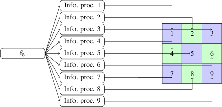
Figure 4: Application of 9 information processing units to expand from one anchor RIS element to 9 RIS elements, where $\mathbf{f}_{5}$ is the channel feature of RIS element 5. Information processing unit 5 is comparable to the information processing units of RISnet with full CSI. Indices of user and layer are omitted for simplicity since the expansion is for RIS elements.

By defining two such expansion layers, the numbers of anchor elements are increased by a factor of 9 in both row and column. If we have 16 RIS elements (4$\times$4) with CSI, we can generate phase shifts of 1296 (36$\times$36) RIS elements.The process of expanding anchor elements is illustrated in Figure 5, where the blue RIS elements in Figure 5(a) can estimate the channel from the pilot signals from the users. Such RIS elements are only 1/81 of all RIS elements. The whole RISnet architecture is shown in Figure 6.

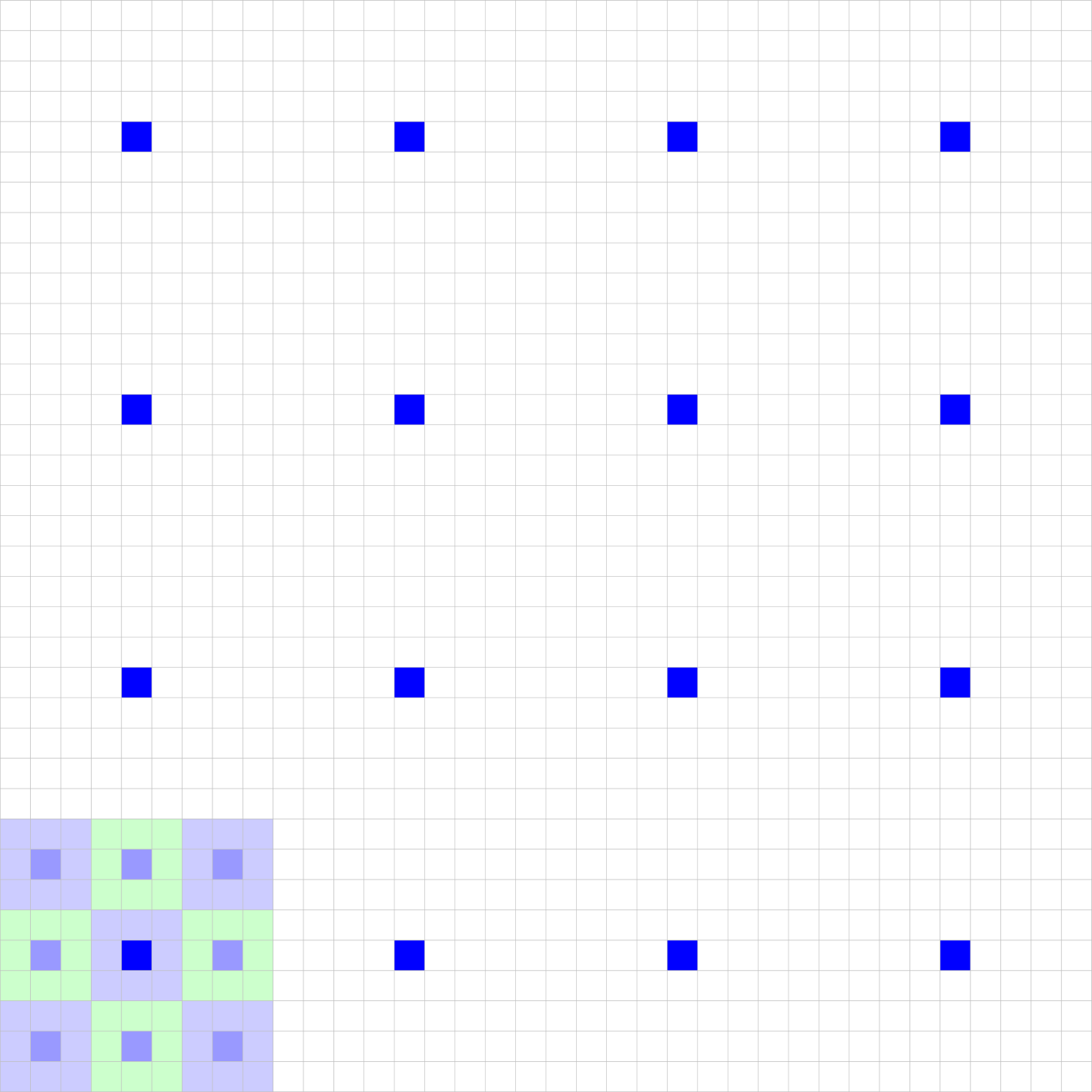
(a) First expansion

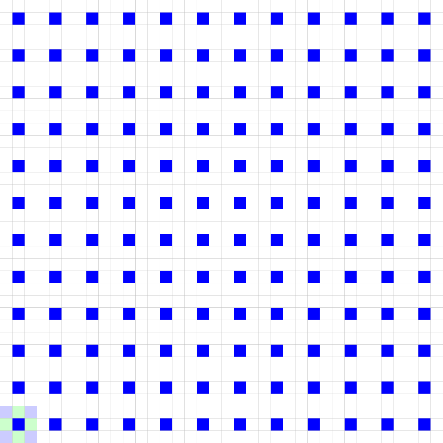
(b) Second expansion

Figure 5: Expansion of considered RIS elements. Blue: anchor RIS elements. Lower left corner: example of the expansion to extend the anchor RIS elements from the blue element to the adjacent elements (light blue elements in Subfigure (a) and all elements in Subfigure (b)).

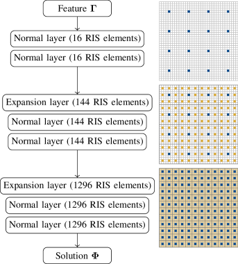
Figure 6: The RISnet architecture with partial CSI, where the information processing of normal layers is given by (26) (SDMA) and (27) (NOMA) and the information processing of expansion layers is given by (28) (SDMA) and (29) (NOMA).

Remark 3.

The RIS elements with the channel estimation capability are fixed once the RIS hardware is designed. Since the hardware design does not change constantly, we assume known and fixed RIS elements with CSI. If the RIS layout is modified, the NN architecture must be modified accordingly. For example, if we want that one element is expanded to the adjacent 25 elements instead of 9, we should define 25 information processing units (see Figure 5).

During the model training, the full CSI is still required to compute the objectives (17a) and (23a). However, phase shifts of all RIS elements $\bm{\Phi}$ are computed with the partial CSI after the training in the application, which implies that only the partial CSI (i.e., an RIS with few RF chains for channel estimation) is required in application.

IV-C4 Efficient Parallel Implementation with Tensor Operations

Although (26), (27), (28) and (29) are the most intuitive way to understand the information flow in RISnet, the computation is done per RIS element (and user), which can only be implemented in a loop and has a low computation efficiency. In order to utilize the parallel computing in a GPU, it would be desirable to implement the information processing as tensor operations instead of computation per RIS element (and user). Let $\mathbf{F}^{ca}_{i+1}$ be the output of information processing unit ca in layer $i$, the second row of the right hand side of (26) can be rewritten as

$$\mathbf{F}^{\text{SDMA},\texttt{ca}}_{i+1}[\cdot,n,u]=\left(\sum_{n^{\prime}}\text{ReLU}(\mathbf{W}^{\texttt{ca}}_{i}\mathbf{f}^{\text{SDMA}}_{un^{\prime},i}+\mathbf{b}_{i}^{\texttt{ca}})\right)/N.$$ (31)

It is easy to prove that (31) is equivalent to

$$\mathbf{F}^{\text{SDMA},\texttt{ca}}_{i+1}=\text{ReLU}(\mathbf{W}^{\texttt{ca}}_{i}\mathbf{F}^{\text{SDMA}}_{i}+\mathbf{b}_{i}^{\texttt{ca}})\cdot\mathbf{1}^{N\times N}/N,$$ (32)

where the multiplication between $\mathbf{W}^{\texttt{ca}}_{i}$ and $\mathbf{F}^{\text{SDMA}}_{i}$ is done in the first dimension (the feature dimension) of $\mathbf{F}^{\text{SDMA}}_{i}$ and the multiplication between $\text{ReLU}(\mathbf{W}^{\texttt{ca}}_{i}\mathbf{F}^{\text{SDMA}}_{i}+\mathbf{b}_{i}^{\texttt{ca}})$ and $\mathbf{1}^{N\times N}$ takes place in the last two dimensions (users and RIS elements) of $\text{ReLU}(\mathbf{W}^{\texttt{ca}}_{i}\mathbf{F}^{\text{SDMA}}_{i}+\mathbf{b}_{i}^{\texttt{ca}})$. In this way, (31) is computed for all RIS elements and users without a loop using tensor operations. Similarly, the third row of the right hand side of (26) can be rewritten as

$$\mathbf{F}^{\text{SDMA},\texttt{oc}}_{i+1}[\cdot,n,u]=\!\!\left(\sum_{u^{\prime}\neq u}\text{ReLU}(\mathbf{W}^{\texttt{oc}}_{i}\mathbf{f}^{\text{SDMA}}_{u^{\prime}n,i}+\mathbf{b}_{i}^{\texttt{oc}})\right)\big{/}(U-1).$$ (33)

It is straightforward to prove that (33) is equivalent to

$$\mathbf{F}^{\text{SDMA},\texttt{oc}}_{i+1}=\mathbf{E}^{U\times U}\cdot\text{ReLU}(\mathbf{W}^{\texttt{oc}}_{i}\mathbf{F}^{\text{SDMA}}_{i}+\mathbf{b}_{i}^{\texttt{oc}})\big{/}(U-1).$$ (34)

Other operations in (26)-(29) can also be parallelized in similar ways. Therefore, the RISnet can be implemented in a computation-efficient way.

IV-D Joint Optimization of BS Precoding and RIS Configuration

Both problems (17) and (23) involve joint optimization of BS precoding and RIS configuration. Since there exist WMMSE precoding for SDMA [8] and precoding for NOMA [5] in quasi-degraded channels, we apply these precoding schemes.

There exists an important difference between the WMMSE precoding and precoding in NOMA: The WMMSE precoding is an iterative approach. In each iteration, a factor $\mu_{k}$ (Equation (18) in [8]) must be computed numerically. Therefore, the WMMSE precoder is indifferentiable and cannot be part of the objective because the NN is trained with gradient ascent. As a result, we apply AO, where we fix the NN and compute the precoding matrix $\mathbf{V}$ for each data sample in $\mathcal{D}$, then treat $\mathbf{V}$ as constants and train the NN for the given precoding.

On the contrary, the precoding for NOMA has a closed-form expression and is differentiable with respect to the channel gains. The objective is a function of channel gains and precoding vectors. The precoding vectors are functions of channel gains. The channel gains are tuned by the phase shifts of the RIS elements, which are output of the NN. Therefore, the objective is the differentiable function composition parameterized by the NN parameters. As a result, we can compute the gradient of the objective with respect to the NN parameters according to the chain rule. The precoding vectors can therefore be part of the objective function.

The training objective for SDMA is simply (17a). For NOMA, we need an additional penalty term to ensure the quasi degradation (QD), which can be intuitively understood as that the achievable rate of the weak user $R_{2}$ is confined by the weak user (i.e., the second term of (22)). Therefore, the objective is defined as

$$\lVert\mathbf{v}_{1}\rVert^{2}+\lVert\mathbf{v}_{2}\rVert^{2}-\lambda\max\left\{0,P\right\},$$ (35)

where $\lambda$ is the factor for the penalty and $P$ is the penalty term [9]:

$$P=\frac{1+r_{1}}{u}-\frac{r_{1}u}{(1+r_{2}(1-u))^{2}}-\frac{||\mathbf{h}_{2}^{2}||^{2}}{||\mathbf{h}_{2}^{2}||^{2}},$$ (36)

with $u=\frac{\mathbf{h}_{2}^{H}\mathbf{h}_{1}\mathbf{h}_{1}^{H}\mathbf{h}_{2}}{||\mathbf{h}_{1}||^{2}||\mathbf{h}_{2}||^{2}}$ and $\mathbf{h}_{u},u=1,2$ being the $u$th row of $\mathbf{C}$.

Summarizing the above descriptions, the algorithms to train the NN is formulated as Algorithm 1 and Algorithm 2.

Algorithm 1 Neural network training with AO for SDMA

1:Initialize the permutation-invariant RISnet $N_{\theta}$.

2:repeat

3:     Randomly choose data samples in a batch.

4:     Compute WMMSE precoding matrix for every data sample, where the precoding matrix is considered as constants for training.

5:     Compute phase shifts $\bm{\Phi}$ with current $N_{\theta}$.

6:     Compute objective (17a) with CSI, user weights, precoding (considered as constants) and phase shifts.

7:     Compute gradient of (17a) with respect to (w.r.t.) $\theta$.

8:     Perform an optimization with the gradient.

9:until convergence

Algorithm 2 Neural network training for NOMA

1:Initialize the permutation-variant RISnet $N_{\theta}$.

2:repeat

3:     Randomly choose data samples in a batch.

4:     Compute phase shifts $\bm{\Phi}$ with current $N_{\theta}$.

5:     Compute the QD penalty for every data sample.

6:     Compute precoding vectors for every data sample, where the precoding vectors are considered as functions of $\theta$.

7:     Compute objective (35) with CSI, rate requirements, precoding (parameterized by $\theta$) and phase shifts.

8:     Compute gradient of (17a) w.r.t. $\theta$.

9:     Perform an optimization with the gradient.

10:until convergence

V Training and Testing Results

The training and testing results are presented in this section. The open-source DeepMIMO data set [42] is applied to generate channel data. The chosen urban scenario is shown in Figure 7, where the LoS channel from BS to users are blocked by a building and only a weak direct channel is available through reflections on buildings and ground. Moreover, the distance between RIS and users is not too large such that the overall channel gain is not too low [43]. Furthermore, the channel from BS to RIS has multiple MPCs such that the MIMO channel matrix has a high rank to support multiple users in SDMA. Finally, we choose users at least 8m from each other for SDMA to realize a full-rank channel matrix from RIS to users and users whose angles-of-arrival are at most 30-Degree away from each other to make QD possible through the RIS. User grouping is assumed given. We note that it is an open topic to assign users according to channel/user positions.

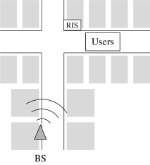
Figure 7: The considered scenario: an intersection in an urban environment.

Important assumptions and parameter settings are listed in Table I. It is to note that the performance is sensitive to the learning rate. In general, a higher learning rate (e.g., $1.5\times 10^{-3}$) is more suitable when considering mutual coupling.

Table I: Scenario and model parameters

Parameter	Value
Number of BS antennas	$9$
RIS size	$36\times 36$ elements
Carrier frequency	$3.5\text{\,}\mathrm{GHz}$
Distance between adjacent antennas at BS	0.5 wavelength
Distance between adjacent antennas at RIS	0.25 wavelength
Number of users	$4$ for SDMA, $2$ for NOMA
Learning rate	$8\times 10^{-4}$ – $1.5\times 10^{-3}$
Batch size	$512$
Optimizer	ADAM
Number of data samples in training set	$10\,240$
Number of data samples in testing set	$1024$

We assume three channel models to assess the feasibility of applying partial CSI for RIS configuration:

• Deterministic ray-tracing channel from DeepMIMO simulator, which is most feasible to infer the full CSI from the partial CSI.

• Deterministic ray-tracing channel plus independent and identically distributed (i.i.d.) channel gains on each RIS element due to the scattering effect. It is less feasible to infer the full CSI from the partial CSI with this model.

• I.i.d. channel model due to scattering of infinitely many infinitely weak propagation paths [44], where the inference of full CSI from partial CSI is impossible.

Figure 8 illustrates the improvement of WSR with SDMA in training and testing with full and partial CSIs, mutual coupling in RIS, and the above-mentioned channel models, where the user weights are uniformly randomly generated and sum up to one. It can be observed that training and testing with the same setup realizes similar performances, suggesting a good generalizability of the trained model. Moreover, similar performances are achieved with full and partial CSI for deterministic channel models and deterministic channel models with i.i.d. scattering gain, suggesting that the partial CSI is sufficient for these scenarios and the difficulty of channel estimation can be relieved a lot, although the performance with partial CSI is moderately worse with the second channel model. On the contrary, the performance with partial CSI in i.i.d. channels is considerably worse than with full CSI, which is expected because partial CSI is insufficient to infer the full CSI if the channels are i.i.d..

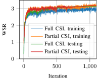
(a) Deterministic ray-tracing channels

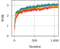
(b) Deterministic ray-tracing channels plus i.i.d. channel gain

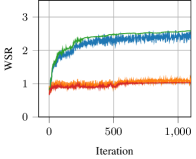
(c) I.i.d. channel gain

Figure 8: Realized WSR in SDMA with mutual coupling in training and testing.

Figure 9 and Figure 10 show the improvement of QD ratio and transmit power assuming mutual coupling in RIS, full and partial CSI and the above-mentioned channel models. Similar observations can be drawn as in Figure 8. It is noticeable that the RIS’s ability to make a channel quasi-degraded is limited and therefore the QD ratio is low with the i.i.d. channel after training (Figure 9(c)). Since the transmit power computation is only valid if the channel is quasi-degraded, this prerequisite is not fulfilled with the i.i.d. channel gain.

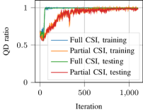
(a) Deterministic ray-tracing channels

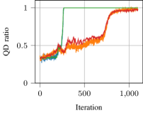
(b) Deterministic ray-tracing channels plus i.i.d. channel gain

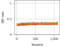
(c) I.i.d. channel gain

Figure 9: Realized quasi-degradation ratio in NOMA with mutual coupling in training and testing.

(a) Deterministic ray-tracing channels

(b) Deterministic ray-tracing channels plus i.i.d. channel gain

(c) I.i.d. channel gain

Figure 10: Realized transmit power in NOMA with mutual coupling in training and testing. Please note the different scalings of the y axis.

Next, we compare our proposed approach with baselines. Since RIS optimization considering mutual coupling for MA is still an open topic, we assume an RIS without mutual coupling and use random phase shifts (for both SDMA and NOMA), BCD algorithm [10] for SDMA and SDR algorithm [15] for NOMA as baselines for comparison. Figure 11 shows the performance comparison of the proposed approach and the baselines. The proposed approach outperforms the baselines considerably with the exception of partial CSI for i.i.d. channels due to the reason explained above. Besides the performance, computing the RIS phase shifts with a trained RISnet takes a few milliseconds compared to more than 20 minutes of the BCD algorithm, suggesting a high feasibility of the RISnet for real time application.

Figure 11: Test result of WSR of models without mutual coupling and baselines.

Figure 12 shows the performances using models trained without and with considerations of mutual coupling for an RIS with mutual coupling and SDMA. When the model is trained without mutual coupling but tested with mutual coupling, the model-mismatch leads to a performance degradation. On the contrary, when mutual coupling is considered in the training, the performance is significantly better. This results justifies the necessity of consideration of mutual coupling in training despite the higher complexity because the mutual coupling does exist in reality.

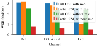
Figure 12: Test result of WSR of models considering and not considering mutual coupling tested with an RIS with mutual coupling.

Figure 13 and Figure 14 show the comparisons between the proposed approach and the baselines for NOMA. Note that the number of RIS elements is reduced to 64 in SDR because the algorithm fails to return a solution with more elements despite multiple attempts of different configurations. This fact shows the advantage in scalability in our approach. Observe that proposed method and SDR are able to realize a QD ratio of (or very close to) 1, and the proposed method (both with full and partial CSI) realizes a significantly lower transmit power.

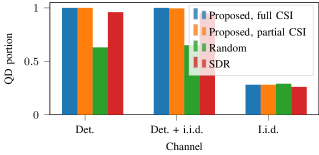
Figure 13: Test result of quasi-degradation ratio of models without mutual coupling and baselines.

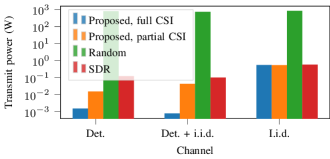
Figure 14: Test result of transmit power of models without mutual coupling and baselines.

Figure 15 and Figure 16 show the performance comparison of models trained with and without consideration of mutual coupling for an RIS with mutual coupling. Unlike SDMA, the performances are similar in NOMA, suggesting that NOMA is less sensitive to RIS mutual coupling.

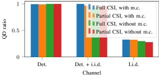
Figure 15: Test result of quasi-degradation ratio of models considering and not considering mutual coupling tested with an RIS with mutual coupling.

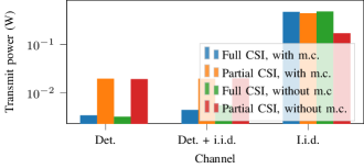
Figure 16: Test result of transmit powers of models considering and not considering mutual coupling tested with an RIS with mutual coupling.

Observing the above results, the feasibility to use partial CSI for RIS configuration depends strongly on the channel model. The partial CSI can be used if the i.i.d. channel gain due to scattering is not dominant, i.e., the channel is sparse, which depends mainly on number, sizes and scatterer roughness and frequency. The more, rougher and smaller the scatterers are in the propagation environment, the more dominant scattering paths there are in the channel [45]. According to [46], the wireless channel is sparse in many typical scenarios, i.e., the signal arrives the receiver via a few distinct MPCs. This fact is the foundation of many compressed sensing based channel estimation [47, 48] and suggests that the proposed method with partial CSI will work in those scenarios.

VI Conclusion

The MA technique is crucial in multi-user wireless communication system. Its performance depends strongly on the channel property, which can be improved by the RIS. In the previous research, scalability of RIS elements, unrealistic assumption of full CSI and ignorance of mutual coupling between adjacent RIS elements are the main limitations of realizing RIS in reality. In this work, we have focused on deriving scalable solutions with unsupervised ML for RIS configuration while making realistic assumptions regarding CSI knowledge and mutual coupling between adjacent RIS elements. We integrate domain-knowledge in communication and ML techniques to design a problem-specific NN architecture RISnet. Moreover, both SDMA and NOMA are addressed within the same framework. In SDMA, user permutation does not impact the performance whereas in NOMA, user decoding order is crucial. This property is addressed in the two variants of RISnet. We further showed that partial CSI is sufficient to achieve a similar performance to full CSI if the channel gain is not dominated by i.i.d. components due to scattering. Finally, we demonstrated that the proposed approach outperforms the baselines significantly and it is necessary to explicitly consider the mutual coupling especially for SDMA. Beyond this work, problem-specific ML combining domain knowledge and ML techniques provides unique opportunity to improve performance, complexity and symmetry compared to generic ML. This work can be extended by considering rate-splitting multiple access (RSMA) and beyond-diagonal RIS.

Appendix A Proof of Theorem 1

We first prove that every layer except the last layer is permutation-equivariant, i.e., if $\mathbf{F}_{i}^{\prime\text{SDMA}}=\mathbf{P}\cdot\mathbf{F}_{i}^{\text{SDMA}}$, where $\mathbf{P}$ is an arbitrary permutation matrix and the multiplication is between $\mathbf{P}$ and the last two dimensions of $\mathbf{F}_{i}^{\text{SDMA}}$, $\mathbf{F}_{i+1}^{\text{SDMA}}=M(\mathbf{F}_{i}^{\text{SDMA}})$ and $\mathbf{F}_{i+1}^{\prime\text{SDMA}}=M(\mathbf{F}_{i}^{\prime\text{SDMA}})$, where $M$ is a layer, we have $\mathbf{F}_{i+1}^{\prime\text{SDMA}}=\mathbf{P}\cdot\mathbf{F}_{i+1}^{\text{SDMA}}$.

We first consider class cc, the output of information processing unit cc of layer $i$ given the permuted input is

$$\mathbf{F}^{\prime\text{SDMA},\texttt{cc}}_{i+1} =\text{ReLU}(\mathbf{W}^{\texttt{cc}}_{i}\mathbf{P}\cdot\mathbf{F}^{\text{SDMA}}_{i}+\mathbf{b}_{i}^{\texttt{cc}})$$ (37)

$$=\text{ReLU}(\mathbf{P}\cdot\mathbf{W}^{\texttt{cc}}_{i}\mathbf{F}^{\text{SDMA}}_{i}+\mathbf{b}_{i}^{\texttt{cc}})$$ (38)

$$=\mathbf{P}\cdot\text{ReLU}(\mathbf{W}^{\texttt{cc}}_{i}\mathbf{F}^{\text{SDMA}}_{i}+\mathbf{b}_{i}^{\texttt{cc}})$$ (39)

$$=\mathbf{P}\mathbf{F}_{i+1}^{\text{SDMA, {cc}}}.$$ (40)

The second line holds because the multiplication with $\mathbf{W}_{i}^{\texttt{cc}}$ is in the first dimension of $\mathbf{P}\cdot\mathbf{F}_{i}^{\text{SDMA}}$, whereas the multiplication with $\mathbf{P}$ is in the second and the third dimensions of $\mathbf{F}_{i}^{\text{SDMA}}$. The third line holds because ReLU is an elementwise operation. The fourth line is the definition of $\mathbf{F}_{i+1}^{\text{SDMA, {cc}}}$. Similarly, we can prove $\mathbf{F}_{i+1}^{\prime\text{SDMA, {ca}}}=\mathbf{P}\cdot\mathbf{F}_{i+1}^{\text{SDMA, {ca}}}$.

To prove $\mathbf{F}_{i+1}^{\prime\text{SDMA, {oc}}}=\mathbf{P}\cdot\mathbf{F}_{i+1}^{\text{SDMA, {oc}}}$, we first need to prove the multiplication between $\mathbf{E}^{U\times U}$ and $\mathbf{P}$ is commutative:

$$\mathbf{E}^{U\times U}\mathbf{P} =\mathbf{1}^{U\times U}\mathbf{P}-\mathbf{I}^{U\times U}\mathbf{P}$$ (41)

$$=\mathbf{P}\mathbf{1}^{U\times U}-\mathbf{P}\mathbf{I}^{U\times U}$$ (42)

$$=\mathbf{P}\mathbf{E}^{U\times U}.$$ (43)

The third line holds because the sum of every row/column of $\mathbf{P}$ is 1. We can now prove the permutation-equivariance as

$$\mathbf{F}^{\prime\text{SDMA},\texttt{oc}}_{i+1} =\mathbf{E}^{U\times U}\cdot\text{ReLU}(\mathbf{W}^{\texttt{oc}}_{i}\mathbf{P}\cdot\mathbf{F}^{\text{SDMA}}_{i}+\mathbf{b}_{i}^{\texttt{oc}})\big{/}(U-1)$$

$$=\mathbf{E}^{U\times U}\cdot\text{ReLU}(\mathbf{P}\cdot\mathbf{W}^{\texttt{oc}}_{i}\mathbf{F}^{\text{SDMA}}_{i}+\mathbf{b}_{i}^{\texttt{oc}})\big{/}(U-1)$$

$$=\mathbf{E}^{U\times U}\mathbf{P}\cdot\text{ReLU}(\mathbf{W}^{\texttt{oc}}_{i}\mathbf{F}^{\text{SDMA}}_{i}+\mathbf{b}_{i}^{\texttt{oc}})\big{/}(U-1)$$

$$=\mathbf{P}\cdot\mathbf{E}^{U\times U}\text{ReLU}(\mathbf{W}^{\texttt{oc}}_{i}\mathbf{F}^{\text{SDMA}}_{i}+\mathbf{b}_{i}^{\texttt{oc}})\big{/}(U-1)$$

$$=\mathbf{P}\cdot\mathbf{F}_{i+1}^{\text{SDMA, {oc}}}.$$

Similarly, we can prove $\mathbf{F}_{i+1}^{\prime\text{SDMA, {oa}}}=\mathbf{P}\cdot\mathbf{F}_{i+1}^{\text{SDMA, {oa}}}$.

Since the output of every class in every layer is permutation-equivariant, the whole output after summation over users is permutation-invariant.

References

- [1] Finn Siegismund-Poschmann, Bile Peng and Eduard A. Jorswieck “Non-orthogonal multiple access assisted by reconfigurable intelligent surface using unsupervised machine learning” In 2023 European Signal Processing Conference (EUSIPCO), 2023
- [2] Bile Peng, Karl-Ludwig Besser, Ramprasad Raghunath, Vahid Jamali and Eduard A. Jorswieck “RISnet: A Scalable Approach for Reconfigurable Intelligent Surface Optimization with Partial CSI” In 2023 IEEE Global Communications Conference (GLOBECOM) IEEE, 2023
- [3] Chun-Yi Wei, Jos Akhtman, Soon Xin Ng and Lajos Hanzo “Iterative near-maximum-likelihood detection in rank-deficient downlink SDMA systems” In IEEE Trans. Veh. Technol. 57.1 IEEE, 2008, pp. 653–657
- [4] Eduard Jorswieck and Sepehr Rezvani “On the Optimality of NOMA in Two-User Downlink Multiple Antenna Channels” In 2021 29th European Signal Processing Conference (EUSIPCO), 2021, pp. 831–835 IEEE
- [5] Zhiyong Chen, Zhiguo Ding, Peng Xu and Xuchu Dai “Optimal precoding for a QoS optimization problem in two-user MISO-NOMA downlink” In IEEE Commun. Lett. 20.6 IEEE, 2016, pp. 1263–1266
- [6] Yuanwei Liu, Xiao Liu, Xidong Mu, Tianwei Hou, Jiaqi Xu, Marco Di Renzo and Naofal Al-Dhahir “Reconfigurable intelligent surfaces: Principles and opportunities” In IEEE Commun. Surv. Tutor. 23.3 IEEE, 2021, pp. 1546–1577
- [7] Michael Joham, Wolfgang Utschick and Josef A Nossek “Linear transmit processing in MIMO communications systems” In IEEE Trans. Signal Process. 53.8 IEEE, 2005, pp. 2700–2712
- [8] Qingjiang Shi, Meisam Razaviyayn, Zhi-Quan Luo and Chen He “An iteratively weighted MMSE approach to distributed sum-utility maximization for a MIMO interfering broadcast channel” In IEEE Trans. Signal Process. 59.9 IEEE, 2011, pp. 4331–4340
- [9] Zhiyong Chen, Zhiguo Ding, Xuchu Dai and George K Karagiannidis “On the application of quasi-degradation to MISO-NOMA downlink” In IEEE Trans. Signal Process. 64.23 IEEE, 2016, pp. 6174–6189
- [10] Huayan Guo, Ying-Chang Liang, Jie Chen and Erik G Larsson “Weighted sum-rate maximization for reconfigurable intelligent surface aided wireless networks” In IEEE Trans. Wirel. Commun. 19.5 IEEE, 2020, pp. 3064–3076
- [11] Chongwen Huang, Alessio Zappone, Mérouane Debbah and Chau Yuen “Achievable rate maximization by passive intelligent mirrors” In 2018 IEEE International Conference on Acoustics, Speech and Signal Processing (ICASSP), 2018, pp. 3714–3718 IEEE
- [12] Gui Zhou, Cunhua Pan, Hong Ren, Kezhi Wang and Arumugam Nallanathan “Intelligent reflecting surface aided multigroup multicast MISO communication systems” In IEEE Trans. Signal Process. 68 IEEE, 2020, pp. 3236–3251
- [13] Xian Liu, Cong Sun and Eduard A Jorswieck “Two-user SINR Region for Reconfigurable Intelligent Surface Aided Downlink Channel” In 2021 IEEE International Conference on Communications Workshops (ICC Workshops), 2021, pp. 1–6 IEEE
- [14] Jianyue Zhu, Yongming Huang, Jiaheng Wang, Keivan Navaie and Zhiguo Ding “Power efficient IRS-assisted NOMA” In IEEE Trans. Commun. 69.2 IEEE, 2020, pp. 900–913
- [15] Min Fu, Yong Zhou and Yuanming Shi “Intelligent reflecting surface for downlink non-orthogonal multiple access networks” In 2019 IEEE Globecom Workshops (GC Wkshps), 2019, pp. 1–6 IEEE
- [16] Gang Yang, Xinyue Xu, Ying-Chang Liang and Marco Di Renzo “Reconfigurable intelligent surface-assisted non-orthogonal multiple access” In IEEE Trans. Wirel. Commun. 20.5 IEEE, 2021, pp. 3137–3151
- [17] Zhengfeng Li, Meng Hua, Qingxia Wang and Qingheng Song “Weighted sum-rate maximization for multi-IRS aided cooperative transmission” In IEEE Wirel. Commun. Lett. 9.10 IEEE, 2020, pp. 1620–1624
- [18] Tianwei Hou, Yuanwei Liu, Zhengyu Song, Xin Sun, Yue Chen and Lajos Hanzo “Reconfigurable intelligent surface aided NOMA networks” In IEEE J. Sel. Areas Commun. 38.11 IEEE, 2020, pp. 2575–2588
- [19] Qingqing Wu and Rui Zhang “Beamforming optimization for wireless network aided by intelligent reflecting surface with discrete phase shifts” In IEEE Trans. Commun. 68.3 IEEE, 2019, pp. 1838–1851
- [20] Ruizhe Long, Ying-Chang Liang, Yiyang Pei and Erik G Larsson “Active reconfigurable intelligent surface-aided wireless communications” In IEEE Trans. Wirel. Commun. 20.8 IEEE, 2021, pp. 4962–4975
- [21] Mohamed A. Elmossallamy, Hongliang Zhang, Radwa Sultan, Karim G. Seddik, Lingyang Song, Zhu Han and Zhu Han “On Spatial Multiplexing Using Reconfigurable Intelligent Surfaces” In IEEE Wirel. Commun. Lett. 10.2, 2021, pp. 226–230 DOI: 10.1109/LWC.2020.3025030
- [22] Marco Di Renzo, Alessio Zappone, Merouane Debbah, Mohamed-Slim Alouini, Chau Yuen, Julien De Rosny and Sergei Tretyakov “Smart radio environments empowered by reconfigurable intelligent surfaces: How it works, state of research, and the road ahead” In IEEE J. Sel. Areas Commun. 38.11 IEEE, 2020, pp. 2450–2525
- [23] Marzieh Najafi, Vahid Jamali, Robert Schober and H Vincent Poor “Physics-based modeling and scalable optimization of large intelligent reflecting surfaces” In IEEE Trans. Commun. 69.4 IEEE, 2020, pp. 2673–2691
- [24] Kurt Hornik, Maxwell Stinchcombe and Halbert White “Multilayer feedforward networks are universal approximators” In Neural Netw. 2.5 Elsevier, 1989, pp. 359–366
- [25] Ruikang Zhong, Yuanwei Liu, Xidong Mu, Yue Chen and Lingyang Song “AI empowered RIS-assisted NOMA networks: Deep learning or reinforcement learning?” In IEEE J. Sel. Areas Commun. 40.1 IEEE, 2021, pp. 182–196
- [26] Xinyu Gao, Yuanwei Liu, Xiao Liu and Lingyang Song “Machine learning empowered resource allocation in IRS aided MISO-NOMA networks” In IEEE Trans. Wirel. Commun. 21.5 IEEE, 2021, pp. 3478–3492
- [27] Xinwei Yue, Jin Xie, Yuanwei Liu, Zhihao Han, Rongke Liu and Zhiguo Ding “Simultaneously transmitting and reflecting reconfigurable intelligent surface assisted NOMA networks” In IEEE Trans. Wirel. Commun. 22.1 IEEE, 2022, pp. 189–204
- [28] Chongwen Huang, Ronghong Mo and Chau Yuen “Reconfigurable intelligent surface assisted multiuser MISO systems exploiting deep reinforcement learning” In IEEE J. Sel. Areas Commun. 38.8 IEEE, 2020, pp. 1839–1850
- [29] Muhammad Shehab, Bekir S Ciftler, Tamer Khattab, Mohamed M Abdallah and Daniele Trinchero “Deep reinforcement learning powered IRS-assisted downlink NOMA” In IEEE Open J. Commun. Soc. 3 IEEE, 2022, pp. 729–739
- [30] Yi Guo, Fang Fang, Donghong Cai and Zhiguo Ding “Energy-efficient design for a NOMA assisted STAR-RIS network with deep reinforcement learning” In IEEE Trans. Veh. Technol. IEEE, 2022
- [31] Baoling Sheen, Jin Yang, Xianglong Feng and Md Moin Uddin Chowdhury “A deep learning based modeling of reconfigurable intelligent surface assisted wireless communications for phase shift configuration” In IEEE Open J. Commun. Soc. 2 IEEE, 2021, pp. 262–272
- [32] Tao Jiang, Hei Victor Cheng and Wei Yu “Learning to reflect and to beamform for intelligent reflecting surface with implicit channel estimation” In IEEE J. Sel. Areas Commun. 39.7 IEEE, 2021, pp. 1931–1945
- [33] Özgecan Özdoğan and Emil Björnson “Deep learning-based phase reconfiguration for intelligent reflecting surfaces” In 2020 54th Asilomar Conference on Signals, Systems, and Computers, 2020, pp. 707–711 IEEE
- [34] Jiancheng An, Chao Xu, Qingqing Wu, Derrick Wing Kwan Ng, Marco Di Renzo, Chau Yuen and Lajos Hanzo “Codebook-based solutions for reconfigurable intelligent surfaces and their open challenges” In IEEE Wirel. Commun. IEEE, 2022
- [35] Xuewen Qian and Marco Di Renzo “Mutual coupling and unit cell aware optimization for reconfigurable intelligent surfaces” In IEEE Wirel. Commun. Lett. 10.6 IEEE, 2021, pp. 1183–1187
- [36] Gabriele Gradoni and Marco Di Renzo “End-to-end mutual coupling aware communication model for reconfigurable intelligent surfaces: An electromagnetic-compliant approach based on mutual impedances” In IEEE Wirel. Commun. Lett. 10.5 IEEE, 2021, pp. 938–942
- [37] Giuseppe Pettanice, Roberto Valentini, Piergiuseppe Di Marco, Fabrizio Loreto, Daniele Romano, Fortunato Santucci, Domenico Spina and Giulio Antonini “Mutual Coupling Aware Time-Domain Characterization and Performance Analysis of Reconfigurable Intelligent Surfaces” In IEEE Trans. Electromagn. Compat. IEEE, 2023
- [38] Shanpu Shen, Bruno Clerckx and Ross Murch “Modeling and architecture design of reconfigurable intelligent surfaces using scattering parameter network analysis” In IEEE Trans. Wirel. Commun. 21.2 IEEE, 2021, pp. 1229–1243
- [39] Matteo Nerini, Shanpu Shen, Hongyu Li, Marco Di Renzo and Bruno Clerckx “A Universal Framework for Multiport Network Analysis of Reconfigurable Intelligent Surfaces”, 2023 arXiv:2311.10561 [cs.IT]
- [40] Tirtharaj Dash, Sharad Chitlangia, Aditya Ahuja and Ashwin Srinivasan “A review of some techniques for inclusion of domain-knowledge into deep neural networks” In Sci. Rep. 12.1 Nature Publishing Group UK London, 2022
- [41] Wei Yu, Foad Sohrabi and Tao Jiang “Role of Deep Learning in Wireless Communications” In IEEE BITS Inf. Theory Mag. 2.2 IEEE, 2022, pp. 56–72 DOI: 10.1109/mbits.2022.3212978
- [42] A. Alkhateeb “DeepMIMO: A Generic Deep Learning Dataset for Millimeter Wave and Massive MIMO Applications” In Proc. of Information Theory and Applications Workshop (ITA), 2019
- [43] Emil Björnson, Özgecan Özdogan and Erik G Larsson “Reconfigurable intelligent surfaces: Three myths and two critical questions” In IEEE Commun. Mag. 58.12 IEEE, 2020, pp. 90–96
- [44] Vahid Jamali, Walid Ghanem, Robert Schober and H Vincent Poor “Impact of Channel Models on Performance Characterization of RIS-Assisted Wireless Systems” In European Conference on Antennas and Propagation (EuCAP), 2023
- [45] Shihao Ju, Syed Hashim Ali Shah, Muhammad Affan Javed, Jun Li, Girish Palteru, Jyotish Robin, Yunchou Xing, Ojas Kanhere and Theodore S Rappaport “Scattering mechanisms and modeling for terahertz wireless communications” In ICC 2019-2019 IEEE International Conference on Communications (ICC), 2019 IEEE
- [46] Akbar M Sayeed “Deconstructing multiantenna fading channels” In IEEE Trans. Signal process. 50.10 IEEE, 2002, pp. 2563–2579
- [47] Saeid Haghighatshoar and Giuseppe Caire “Massive MIMO pilot decontamination and channel interpolation via wideband sparse channel estimation” In IEEE Trans. Wirel. Commun. 16.12 IEEE, 2017, pp. 8316–8332
- [48] Gerhard Wunder, Stelios Stefanatos, Axel Flinth, Ingo Roth and Giuseppe Caire “Low-overhead hierarchically-sparse channel estimation for multiuser wideband massive MIMO” In IEEE Trans. Wirel. Commun. 18.4 IEEE, 2019, pp. 2186–2199