Stability Analysis of Feedback Systems with
ReLU Nonlinearities via
Semialgebraic Set Representation

Abstract

This paper is concerned with the stability analysis problem of feedback systems with rectified linear unit (ReLU) nonlinearities. Such feedback systems arise when we model dynamical (recurrent) neural networks (NNs) and NN-driven control systems where all the activation functions of NNs are ReLUs. In this study, we focus on the semialgebraic set representation characterizing the input-output properties of ReLUs. This allows us to employ a novel copositive multiplier in the framework of the integral quadratic constraint and, thus, to derive a linear matrix inequality (LMI) condition for the stability analysis of the feedback systems. However, the infeasibility of this LMI does not allow us to obtain any conclusion on the system’s stability due to its conservativeness. This motivates us to consider its dual LMI. By investigating the structure of the dual solution, we derive a rank condition on the dual variable certificating that the system at hand is never stable. In addition, we construct a hierarchy of dual LMIs allowing for improved instability detection. We illustrate the effectiveness of the proposed approach by several numerical examples.

1 Introduction

Control theoretic approaches for the analysis and synthesis of neural networks (NNs) (Fazlyab et al. (2022); Raghunathan et al. (2018); Revay et al. (2021); Grönqvist and Rantzer (2022); Ebihara et al. (2021, 2024)) and of dynamical systems driven by NNs (Yin et al. (2022); Scherer (2022)) have attracted great attention recently. In this study, we are particularly interested in dynamical NNs such as recurrent NNs (RNNs) and NN-driven control systems where the activation functions in NNs are rectified linear units (ReLUs). Such systems can be regarded as a special class of Lurie systems for which effective analysis and synthesis conditions have been developed, see, e.g., Tarbouriech et al. (2011). The generality of the approaches for Lurie systems comes at the expense of strong conservativeness, and studies specialized to ReLU nonlinearity are relatively scarce. Hence, in this paper, we aim to derive analysis conditions that are specific to ReLU nonlinearity.

In this paper, we focus on the semialgebraic set representation that accurately characterizes the input-output properties of ReLUs (Raghunathan et al. (2018); Groff et al. (2019)). By focusing on this semialgebraic set representation, in Ebihara et al. (2024), we have already introduced what we call “copositive multiplier” that captures the input-output properties in quadratic form. By using this novel multiplier in the general framework of integral quadratic constraint (IQC) theory (Megretski and Rantzer (1997); Scherer (2022)), we first derive a (primal) linear matrix inequality (LMI) condition for the stability analysis of the feedback systems with ReLU nonlinearities. However, this primal LMI is conservative in general. Therefore, if the primal LMI turns out to be infeasible by numerical computation, we cannot conclude anything about the system’s stability. This motivates us to focus on the dual LMI whose feasibility is guaranteed by the theorems of alternative. By closely investigating the structure of the dual solution, we then obtain a rank condition on the dual variable under which we can conclude that the feedback system is never stable. Moreover, from the dual solution satisfying the rank condition, we can extract an initial condition from which the state trajectory does not converge to the origin. In robust stability analysis of linear dynamical systems affected by parametric uncertainties, it is well known that dual LMIs are quite useful in extracting worst-case parameters that destabilize the systems, see, e.g., Scherer (2005); Masubuchi and Scherer (2009); Ebihara et al. (2009). In the present paper, the dual LMI works effectively in extracting the worst-case initial condition for nonlinear systems in the above sense. We also show that the dual LMI can be interpreted as an LMI relaxation of a system of algebraic inequalities that characterizes the existence of the worst-case initial conditions. This interpretation and the semialgebraic set representation, together with the idea of employing dual variables of block-Hankel matrix structure in Ebihara et al. (2009), enable us to construct a hierarchy of dual LMIs with which the detection of the worst-case initial condition is more likely to be expected. We illustrate the effectiveness of the proposed approach by several numerical examples.

Notation: The set of $\displaystyle n\times m$ real matrices is denoted by $\displaystyle{\mathbb{R}}^{n\times m}$, and the set of $\displaystyle n\times m$ entrywise nonnegative matrices is denoted by $\displaystyle{\mathbb{R}}_{+}^{n\times m}$. For a matrix $\displaystyle A$, we also write $\displaystyle A\geq 0$ to denote that $\displaystyle A$ is entrywise nonnegative. We denote the set of $\displaystyle n\times n$ real symmetric, positive semidefinite (definite), and Hurwitz stable matrices by $\displaystyle{\mathbb{S}}^{n}$, $\displaystyle{\mathbb{S}}_{+}^{n}$ ($\displaystyle{\mathbb{S}}_{++}^{n}$), and $\displaystyle{\mathbb{H}}^{n}$, respectively. For $\displaystyle A\in{\mathbb{S}}^{n}$, we also write $\displaystyle A\succ 0\ (A\prec 0)$ to denote that $\displaystyle A$ is positive (negative) definite. For $\displaystyle A\in{\mathbb{R}}^{n\times n}$, we define $\displaystyle{\rm He}\{A\}:=A+A^{T}$ and $\displaystyle{\rm diag}(A)\in{\mathbb{R}}^{n}$ where $\displaystyle({\rm diag}(A))_{i}:=A_{i,i}\ (i=1,\cdots,n)$. For $\displaystyle A\in{\mathbb{R}}^{n\times n}$ and $\displaystyle B\in{\mathbb{R}}^{n\times m}$, $\displaystyle(\ast)^{T}AB$ is a shorthand notation of $\displaystyle B^{T}AB$. We denote by $\displaystyle{\mathbb{D}}^{n}\subset{\mathbb{R}}^{n\times n}$ the set of diagonal matrices. For $\displaystyle v\in{\mathbb{R}}^{n}$, $\displaystyle\|v\|$ stands for the standard Euclidean norm. For a static (possibly nonlinear) operator $\displaystyle\Psi:\ {\mathbb{R}}^{n}\mapsto{\mathbb{R}}^{m}$, we denote by $\displaystyle\|\Psi\|$ its $\displaystyle l_{2}$-induced norm. We define the positive semidefinite cone $\displaystyle{\mathcal{PSD}}^{n}\subset{\mathbb{S}}^{n}$, the copositive cone $\displaystyle{\mathcal{COP}}^{n}\subset{\mathbb{S}}^{n}$, and the nonnegative cone $\displaystyle{\mathcal{NN}}^{n}\subset{\mathbb{S}}^{n}$ as follows:

$$\begin{array}[]{@{}l}{\mathcal{PSD}}^{n}:=\{P\in{\mathbb{S}}^{n}:\ x^{T}Px\geq 0\ \forall x\in{\mathbb{R}}^{n}\},\\ {\mathcal{COP}}^{n}:=\{P\in{\mathbb{S}}^{n}:\ x^{T}Px\geq 0\ \forall x\in{\mathbb{R}}_{+}^{n}\},\\ {\mathcal{NN}}^{n}:=\{P\in{\mathbb{S}}^{n}:\ P\geq 0\}.\end{array}$$

We can readily see that $\displaystyle{\mathcal{PSD}}^{n}\subset{\mathcal{PSD}}^{n}+{\mathcal{NN}}^{n}\subset{\mathcal{COP}}^{n}$, where “$\displaystyle+$” here stands for the Minkowski sum.

2 Problem Setting and
Preliminary Results

Figure 1: Nonlinear Feedback System $\displaystyle\Sigma$.

Let us consider the feedback system $\displaystyle\Sigma$ shown in Fig. 1. Here, $\displaystyle G$ is a linear system described by

$$G:\ \left\{\begin{array}[]{lcl}\dot{x}(t)&=&Ax(t)+Bw(t),\\ z(t)&=&Cx(t)+Dw(t)\end{array}\right.$$ (1)

where $\displaystyle A\in{\mathbb{R}}^{n\times n}\cap{\mathbb{H}}^{n}$, $\displaystyle B\in{\mathbb{R}}^{n\times m}$, $\displaystyle C\in{\mathbb{R}}^{m\times n}$, and $\displaystyle D\in{\mathbb{R}}^{m\times m}$. Moreover, we have

$$w(t)=\Phi(z(t)),$$ (2)

where $\displaystyle\Phi:\ {\mathbb{R}}^{m}\mapsto{\mathbb{R}}^{m}$ stands for the static rectified linear unit (ReLU) nonlinearity given by

$$\begin{array}[]{@{}l}\Phi(q)=\left[\ \phi(q_{1})\ \cdots\ \phi(q_{m})\ \right]^{T},\\ \phi:{\mathbb{R}}\to{\mathbb{R}},\quad\phi(\eta)=\left\{\begin{array}[]{cc}\eta&(\eta\geq 0),\\ 0&(\eta<0).\\ \end{array}\right.\end{array}$$ (3)

Remark 1

We note that ReLU $\displaystyle\Phi:{\mathbb{R}}^{m}\mapsto{\mathbb{R}}^{m}$ satisfies

$$\Phi(\alpha q)=\alpha\Phi(q)\ \forall(\alpha,q)\in{\mathbb{R}}_{+}\times{\mathbb{R}}^{m}.$$ (4)

In addition, for $\displaystyle p,q\in{\mathbb{R}}^{m}$, it is shown in Raghunathan et al. (2018) and Groff et al. (2019) that $\displaystyle p=\Phi(q)$ holds if and only if

$$p-q\geq 0,\ p\geq 0,\ (p-q)\odot p=0$$ (5)

where $\displaystyle\odot$ stands for the Hadamard product. Namely, the input-output properties of the ReLU $\displaystyle\Phi$ can be accurately characterized by the semialgebraic set (5).

It can be easily seen that $\displaystyle\|\Phi\|=1$. With this fact in mind, for the well-posedness of the feedback system $\displaystyle\Sigma$, we assume $\displaystyle\|D\|<1$. Under this assumption, we see that the map $\displaystyle(I-D\Phi):\ {\mathbb{R}}^{m}\mapsto{\mathbb{R}}^{m}$ is invertible and hence the inverse map $\displaystyle(I-D\Phi)^{-1}:\ {\mathbb{R}}^{m}\mapsto{\mathbb{R}}^{m}$ is well defined. Moreover, the next results follow.

Lemma 1

Suppose $\displaystyle\|D\|<1$. Then, we can represent the dynamics of the system $\displaystyle\Sigma$ by

$$\Sigma:\ \dot{x}(t)=Ax(t)+B\Phi\circ(I-D\Phi)^{-1}(Cx(t)).$$ (6)

In addition, we have

$$(I-D\Phi)^{-1}(\alpha q)=\alpha(I-D\Phi)^{-1}(q)\ \forall(\alpha,q)\in{\mathbb{R}}_{+}\times{\mathbb{R}}^{m}.$$ (7)

Proof of Lemma 7: It is obvious that (6) holds. For the proof of (7), for given $\displaystyle q\in{\mathbb{R}}^{m}$, we first define

$$p:=(I-D\Phi)^{-1}(q).$$

This implies $\displaystyle q=(I-D\Phi)(p)$. Then, for given $\displaystyle\alpha\in{\mathbb{R}}_{+}$, we have from (4) that

$$\alpha q=\alpha(I-D\Phi)(p)=(I-D\Phi)(\alpha p).$$

This clearly shows that (7) holds.   

This paper addresses the stability analysis problem of the system $\displaystyle\Sigma$. The definition of “stability” is now recalled.

Definition 1 (Khalil (2002))

The equilibrium point $\displaystyle x=0$ (i.e., the origin) of the feedback system $\displaystyle\Sigma$ given by (6) is said to be locally asymptotically stable if the conditions (i) and (ii) given below are satisfied, and is said to be globally asymptotically stable if the conditions (i) and (iii) given below are satisfied, where

• for each $\displaystyle\varepsilon>0$, there exists $\displaystyle\delta=\delta(\varepsilon)>0$ such that

  $$\|x(0)\|<\delta\ \Rightarrow\ \|x(t)\|<\varepsilon\ (\forall t\geq 0);$$

• there exist $\displaystyle\delta>0$ such that

  $$\|x(0)\|<\delta\ \Rightarrow\ \lim_{t\to\infty}x(t)=0;$$

• $\displaystyle\lim_{t\to\infty}x(t)=0$ holds for any $\displaystyle x(0)$.

For general nonlinear feedback systems, it is of course true that there is a clear distinction between the local and global asymptotic stability. However, for the nonlinear feedback system $\displaystyle\Sigma$ with ReLU nonlinearities, they are equivalent as shown in the next theorem.

Theorem 1

The nonlinear feedback system $\displaystyle\Sigma$ given by (6) is globally asymptotically stable if and only if it is locally asymptotically stable.

Proof of Theorem 1: Let us define the state trajectory of (6) for the initial state $\displaystyle x(0)=\xi$ by $\displaystyle x_{\xi}(t)\ (t\geq 0)$. Then, from the definition of the local and global asymptotic stability given in Definition 1, we see that Theorem 1 is verified by showing that $\displaystyle x_{\alpha\xi}(t)=\alpha x_{\xi}(t)$ holds for any $\displaystyle\alpha\in{\mathbb{R}}_{+}$. This can be readily validated since

$$\frac{d}{dt}(\alpha x_{\xi}(t)) =\alpha\dot{x}_{\xi}(t)$$

$$=\alpha\left(Ax_{\xi}(t)+B\Phi\circ(I-D\Phi)^{-1}(Cx_{\xi}(t))\right)$$

$$=A(\alpha x_{\xi}(t))+B\Phi\circ(I-D\Phi)^{-1}(C(\alpha x_{\xi}(t)))$$

where we used (4) and (7). This clearly shows that $\displaystyle x_{\alpha\xi}(t)=\alpha x_{\xi}(t)$ holds and hence the proof is completed.   

On the basis of Theorem 1, we investigate the global asymptotic stability analysis of the feedback system $\displaystyle\Sigma$. For simplicity, we say that the feedback system $\displaystyle\Sigma$ is stable if it is globally asymptotically stable. The next proposition forms the basis for the stability analysis using integral quadratic constraint (IQC) theory.

Proposition 1 (Megretski and Rantzer (1997))

Let us define $\displaystyle{{\mathbf{\Pi}}^{\star}}\subset{\mathbb{S}}^{2m}$ by

$$\begin{array}[]{@{}l}{{\mathbf{\Pi}}^{\star}}:=\left\{\Pi\in{\mathbb{S}}^{2m}:\ \left[\begin{array}[]{c}\zeta\\ \xi\\ \end{array}\right]^{T}\Pi\left[\begin{array}[]{c}\zeta\\ \xi\\ \end{array}\right]\geq 0\right.\\ \left.\hskip 28.45274pt\forall\left[\begin{array}[]{c}\zeta\\ \xi\\ \end{array}\right]\in{\mathbb{R}}^{2m}\ \mathrm{s.t.}\ \xi=\Phi(\zeta)\right\}.\end{array}$$ (8)

Then, the system $\displaystyle\Sigma$ is stable if there exist $\displaystyle P\succ 0$ and $\displaystyle\Pi\in{{\mathbf{\Pi}}^{\star}}$ such that

$$\begin{bmatrix}PA+A^{T}P&PB\\ B^{T}P&0\end{bmatrix}+\begin{bmatrix}C&D\\ 0&I_{m}\end{bmatrix}^{T}\Pi\begin{bmatrix}C&D\\ 0&I_{m}\end{bmatrix}\prec 0.$$ (9)

3 Multipliers Capturing
Input-Output Properties of ReLU

In the IQC-based stability condition (9), it is of prime importance to employ a set of multipliers $\displaystyle\boldsymbol{\Pi}\subset\boldsymbol{\Pi}^{\star}$ that is numerically tractable and captures the input-output properties of ReLU $\displaystyle\Phi$ as accurately as possible. On this issue, the next results have been obtained recently.

Proposition 2 (Ebihara et al. (2024))

Let us define $\displaystyle\boldsymbol{\Pi}_{\mathcal{COP}},\boldsymbol{\Pi}_{\mathcal{NN}}\subset{\mathbb{S}}^{2m}$ by

Then we have $\displaystyle\boldsymbol{\Pi}_{\mathcal{NN}}\subset\boldsymbol{\Pi}_{\mathcal{COP}}\subset\boldsymbol{\Pi}^{\star}$.

Propositions 9 and 2 enable us to derive a concrete LMI for the stability analysis of the system $\displaystyle\Sigma$; see “Primal LMI” in Theorem 2 in the next section.

The validity of employing $\displaystyle Q\in{\mathcal{COP}}^{2m}$ in $\displaystyle{\mathbf{\Pi}}_{\mathcal{COP}}$ (or $\displaystyle Q\in{\mathcal{NN}}^{2m}$ in $\displaystyle{\mathbf{\Pi}}_{\mathcal{NN}}$) can be seen from the first and the second inequality constraints in the semialgebraic set representation (5), and the validity of employing $\displaystyle J\in{\mathbb{D}}^{n}$ in $\displaystyle{\mathbf{\Pi}}_{\mathcal{COP}}$ and $\displaystyle{\mathbf{\Pi}}_{\mathcal{NN}}$ can be seen from the third equality constraint in (5).

As mentioned in Dür (2010), the problem of determining whether a given matrix is copositive or not is a co-NP complete problem in general, and hence the set of multipliers $\displaystyle\boldsymbol{\Pi}_{\mathcal{COP}}$ is numerically intractable. We therefore employ $\displaystyle\boldsymbol{\Pi}_{\mathcal{NN}}$ in this paper. Since the ReLU $\displaystyle\Phi$ is a (repeated) slope-restricted nonlinearity, we can also employ known multipliers that are valid for this class of nonlinearities such as (static) O’Shea-Zames-Falb multipliers (O’Shea (1967); Zames and Falb (1968); Carrasco et al. (2016); Fetzer and Scherer (2017)) and the multipliers proposed by Fazlyab et al. (Fazlyab et al. (2022)). It has been shown that $\displaystyle\boldsymbol{\Pi}_{\mathcal{NN}}$ encompasses these known multipliers; see Ebihara et al. (2024) for details.

4 Main Results: Primal/Dual LMIs for Stability/Instability Certificate

On the basis of Propositions 9 and 2, we can obtain the next results.

Theorem 2

Let us consider the primal and dual LMIs given respectively as follows:
Primal LMI:

$$\mathrm{Find}\ P\in{\mathbb{S}}_{++}^{n}\ \mathrm{and}\ \Pi\in\boldsymbol{\Pi}_{\mathcal{NN}}\ \mathrm{such\ that}\ \eqref{eq:stab}.$$ (11)

Dual LMI:

$$\begin{array}[]{@{}l}\mathrm{Find}\ H=\begin{bmatrix}H_{11}&H_{12}\\ H_{12}^{T}&H_{22}\end{bmatrix}\in{\mathbb{S}}_{+}^{n+m}\setminus\{0\}\ \mathrm{such\ that}\\ {\rm He}\{AH_{11}+BH_{12}^{T}\}\succeq 0,\\ \begin{bmatrix}-C&-D+I_{m}\\ 0&I_{m}\end{bmatrix}H\begin{bmatrix}-C&-D+I_{m}\\ 0&I_{m}\end{bmatrix}^{T}\geq 0,\\ {\rm diag}(-CH_{12}+(-D+I_{m})H_{22})=0.\end{array}$$ (12)

Then, the system $\displaystyle\Sigma$ is stable if the primal LMI (11) is feasible. In addition, the primal LMI (11) is infeasible if and only if the dual LMI (12) is feasible.

The dual LMI (12) can be derived from the primal LMI (11) by following the Lagrange duality theory for semidefinite programming problems (Scherer (2006)). The last assertion in Theorem 2 also follows from theorems of alternative for LMIs; see, e.g., Scherer (2006).

If the primal LMI (11) is feasible, we can conclude that the system $\displaystyle\Sigma$ is stable. However, if the primal LMI (11) is infeasible, we cannot conclude anything. This motivates us to focus on the dual LMI (12) that is always feasible in this case as shown in Theorem 2. In fact, by paying attention to the structure of the dual solution, we can obtain the next theorem that is the first main result of this paper.

Theorem 3

Suppose the dual LMI (12) is feasible with a dual solution $\displaystyle H\in{\mathbb{S}}_{+}^{n+m}\setminus\{0\}$ of $\displaystyle{\rm rank}(H)=1$. Then, the system $\displaystyle\Sigma$ is not stable. Moreover, the following assertions hold:

• The full-rank factorization of $\displaystyle H$ is given of the form

  $$H=\begin{bmatrix}h_{1}\\ h_{2}\end{bmatrix}\begin{bmatrix}h_{1}\\ h_{2}\end{bmatrix}^{T},\ h_{1}\in{\mathbb{R}}^{n},\ h_{2}\in{\mathbb{R}}_{+}^{m}.$$ (13)

• The state $\displaystyle x$ of the system $\displaystyle\Sigma$ corresponding to the initial state $\displaystyle x(0)=h_{1}$ does not satisfy $\displaystyle\lim_{t\to\infty}x(t)\to 0$.

For the proof of this theorem, we need the next lemma.

Lemma 2 (Ebihara (2012))

For given $\displaystyle f,g\in{\mathbb{R}}^{n}$ with $\displaystyle f\neq 0$, the following conditions are equivalent:

• $\displaystyle{\rm He}\{fg^{T}\}\succeq 0$.

• There exists $\displaystyle\lambda\in{\mathbb{R}}^{+}$ such that $\displaystyle g=\lambda f$.

Proof of Theorem 3: We first prove (13). Since $\displaystyle{\rm rank}(H)=1$ holds, its full-rank factorization is given of the form

$$H=\begin{bmatrix}h_{1}\\ h_{2}\end{bmatrix}\begin{bmatrix}h_{1}\\ h_{2}\end{bmatrix}^{T},\ h_{1}\in{\mathbb{R}}^{n},\ h_{2}\in{\mathbb{R}}^{m}.$$

Then, from the second constraint in (12), we have

$$\begin{bmatrix}h_{2}-(Ch_{1}+Dh_{2})\\ h_{2}\end{bmatrix}\begin{bmatrix}h_{2}-(Ch_{1}+Dh_{2})\\ h_{2}\end{bmatrix}^{T}\geq 0.$$

Therefore we see

$$\begin{bmatrix}h_{2}-(Ch_{1}+Dh_{2})\\ h_{2}\end{bmatrix}\geq 0\ \mathrm{or}\ \begin{bmatrix}h_{2}-(Ch_{1}+Dh_{2})\\ h_{2}\end{bmatrix}\leq 0,$$

but this implies that (by changing the sign of $\displaystyle h_{1}$ and $\displaystyle h_{2}$ if necessary) we can always choose $\displaystyle h_{1}$ and $\displaystyle h_{2}$ such that

$$\begin{bmatrix}h_{2}-(Ch_{1}+Dh_{2})\\ h_{2}\end{bmatrix}\geq 0.$$ (14)

This shows that (13) holds.

In addition, the third constraint in (12) reduces to

$$(h_{2}-(Ch_{1}+Dh_{2}))\odot h_{2}=0.$$ (15)

From (14) and (15) together with the semialgebraic set representation (5), we see

$$h_{2}=\Phi(Ch_{1}+Dh_{2}).$$ (16)

On the other hand, the first constraint in (12) reduces to

$${\rm He}\{(Ah_{1}+Bh_{2})h_{1}^{T}\}\succeq 0.$$ (17)

Here we first prove $\displaystyle h_{1}\neq 0$ by contradiction. To this end, suppose $\displaystyle h_{1}=0$. Then, from the underlying assumption that $\displaystyle H\neq 0$, we see $\displaystyle h_{2}\neq 0$. Then, we see that (15) reduces to $\displaystyle(h_{2}-Dh_{2})\odot h_{2}=0$ and this implies $\displaystyle h_{2}^{T}h_{2}=h_{2}^{T}Dh_{2}$. However, this cannot hold for $\displaystyle h_{2}\neq 0$ from our assumption that $\displaystyle\|D\|<1$. Then, by contradiction, we have $\displaystyle h_{1}\neq 0$.

Since $\displaystyle h_{1}\neq 0$ as proved, we see from Lemma 2 and (17) that there exists $\displaystyle\lambda\in{\mathbb{R}}_{+}$ such that

$$Ah_{1}+Bh_{2}=\lambda h_{1}.$$ (18)

We are now in the right position to complete the proof. To validate the assertion (ii), it suffices to show that the state trajectory $\displaystyle x(t)$ of the system $\displaystyle\Sigma$ given by (6) with the initial condition $\displaystyle x(0)=h_{1}$ is given by $\displaystyle x(t)=e^{\lambda t}h_{1}$. From (18), (16), and (4), we have

$$\begin{array}[]{@{}lcl}\displaystyle\frac{d}{dt}x(t)&=&e^{\lambda t}\lambda h_{1}\\ &=&e^{\lambda t}\left(Ah_{1}+Bh_{2}\right)\\ &=&Ae^{\lambda t}h_{1}+Be^{\lambda t}h_{2}\\ &=&Ax(t)+Be^{\lambda t}\Phi(Ch_{1}+Dh_{2})\\ &=&Ax(t)+B\Phi(Ce^{\lambda t}h_{1}+De^{\lambda t}h_{2})\\ &=&Ax(t)+B\Phi(z(t))\\ \end{array}$$ (19)

where

$$\begin{array}[]{@{}lcl}\displaystyle z(t)&=&Ce^{\lambda t}h_{1}+De^{\lambda t}h_{2}\\ &=&Cx(t)+De^{\lambda t}\Phi(Ch_{1}+Dh_{2})\\ &=&Cx(t)+D\Phi(Ce^{\lambda t}h_{1}+De^{\lambda t}h_{2})\\ &=&Cx(t)+D\Phi(z(t)).\end{array}$$

It follows that $\displaystyle z(t)=(I-D\Phi)^{-1}(Cx(t))$. By substituting this into (19), we see that $\displaystyle x(t)=e^{\lambda t}h_{1}$ surely satisfies (6). This completes the proof.   

Remark 2

For robust stability analysis problems of linear dynamical systems affected by parametric uncertainties, it is well known that dual LMIs are useful in extracting worst-case parameters that destabilize the system, see, e.g., Scherer (2005); Masubuchi and Scherer (2009); Ebihara et al. (2009). In the present result for the stability analysis of the nonlinear feedback system $\displaystyle\Sigma$, the dual LMI (12) works effectively in extracting a worst-case initial condition from which the state trajectory does not converge to the origin.

5 Numerical Examples

The systems considered in the examples in this section and Subsection 6.3 are chosen to simulate the typical situation of the stability analysis of RNNs and NN-driven control systems. If we employ a ReLU-RNN as a model of a complex dynamical system, we typically employ a large number of ReLUs to imitate the complex behavior. In addition, for a plant subject to unknown nonlinearities, we often employ a dynamical ReLU-NN as a controller again with a large number of ReLUs to approximate the unknown nonlinearities. In such cases, the system of interest will be described by (1) and (2) where $\displaystyle m>n$.

5.1 The Case $\displaystyle D\neq 0$ and Primal LMI Feasible

Let us consider the case where $\displaystyle n=2$, $\displaystyle m=5$ in (1) and

For this system, the primal LMI (11) turns out to feasible, thereby we can conclude that the system $\displaystyle\Sigma$ is stable. Fig. 4 shows the vector field of system $\displaystyle\Sigma$, together with the state trajectories from the initial states $\displaystyle x(0)=[\ 3\ 3\ ]^{T}$ and $\displaystyle x(0)=[\ -3\ -3\ ]^{T}$. The state trajectories converge to the origin. In this example, the LMI (9) with the set of O’Shea-Zames-Falb multipliers employing doubly hyperdominant matrices turns out to be infeasible. This shows the usefulness of the new set of multipliers $\displaystyle\boldsymbol{\Pi}_{\mathcal{NN}}$ proposed in Proposition 2.

5.2 The Case $\displaystyle D=0$ and Dual LMI Feasible

Let us consider the case where $\displaystyle n=2$, $\displaystyle m=5$ in (1) and

For this system, the dual LMI (12) turns out to be feasible, and the resulting dual solution $\displaystyle H$ is numerically verified to be $\displaystyle{\rm rank}(H)=1$. Therefore we can conclude that the system $\displaystyle\Sigma$ is not stable. The full-rank factorization of $\displaystyle H$ of the form (13) and $\displaystyle\lambda\in{\mathbb{R}}_{+}$ are given by

$$h_{1}=\begin{bmatrix}[r]-0.6282\\ -0.7780\end{bmatrix},\ h_{2}=\begin{bmatrix}[r]0.0000\\ 0.3414\\ 0.0000\\ 0.0000\\ 0.0000\end{bmatrix},\ \lambda=0.1037.$$

Fig. 4 shows the vector field of system $\displaystyle\Sigma$, together with the state trajectories from initial states $\displaystyle x(0)=h_{1}$ and $\displaystyle x(0)=[\ 1\ 1\ ]^{T}$. The state trajectory from the initial state $\displaystyle x(0)=[\ 1\ 1\ ]^{T}$ converges to the origin. However, as proved in Theorem 3, the state trajectory from the initial state $\displaystyle x(0)=h_{1}$ does not converge to the origin (and in this case diverges).

5.3 The Case $\displaystyle D\neq 0$ and Dual LMI Feasible

Let us consider the case where $\displaystyle n=2$, $\displaystyle m=5$ in (1) and

For this system, the dual LMI (12) turns out to be feasible, and the resulting dual solution $\displaystyle H$ is numerically verified to be $\displaystyle{\rm rank}(H)=1$. Therefore we can conclude that the system $\displaystyle\Sigma$ is not stable. The full-rank factorization of $\displaystyle H$ and $\displaystyle\lambda\in{\mathbb{R}}_{+}$ are given by

$$h_{1}=\begin{bmatrix}[r]0.6119\\ 0.7909\\ \end{bmatrix},\ h_{2}=\begin{bmatrix}[r]0.0000\\ 0.0000\\ 0.0000\\ 0.0000\\ 0.2932\\ \end{bmatrix},\ \lambda=0.0807.$$

Fig. 4 shows the vector field of system $\displaystyle\Sigma$, together with the state trajectories from initial states $\displaystyle x(0)=h_{1}$ and $\displaystyle x(0)=[\ -1\ -1\ ]^{T}$. The state trajectory from the initial state $\displaystyle x(0)=[\ -1\ -1\ ]^{T}$ converges to the origin. However, as proved in Theorem 3, the state trajectory from the initial state $\displaystyle x(0)=h_{1}$ does not converge to the origin (and in this case diverges).

We finally note that, from the comparison between Figs. 4, 4 and Fig. 4, we can recognize that the appearance of the vector fields with $\displaystyle D\neq 0$ becomes more complicated than that of $\displaystyle D=0$.

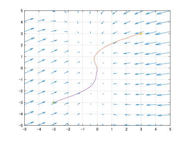
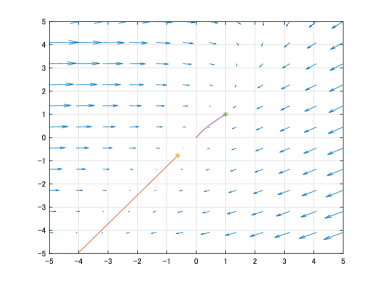
Figure 2: State trajectories from initial conditions $\displaystyle x(0)=[\ 3\ 3\ ]^{T}$ and $\displaystyle x(0)=[\ -3\ -3\ ]^{T}$.

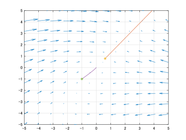
Figure 3: State trajectories from initial conditions $\displaystyle x(0)=h_{1}$ and $\displaystyle x(0)=[\ 1\ 1\ ]^{T}$.

Figure 4: State trajectories from initial conditions $\displaystyle x(0)=h_{1}$ and $\displaystyle x(0)=[\ -1\ -1\ ]^{T}$.

6 Interpretation of Dual LMI and
Higher Order LMI Relaxations

6.1 Interpretation of Dual LMI

The dual LMI (12) and the proof of Theorem 3 together with the semialgebraic set representation (5) motivate us to consider the following algebraic inequality feasibility problem:

Find $\displaystyle h_{1}\in{\mathbb{R}}^{n},\ h_{2}\in{\mathbb{R}}_{+}^{m},\ \lambda\in{\mathbb{R}}_{+}$ such that

$$\begin{array}[]{@{}l}Ah_{1}+Bh_{2}=\lambda h_{1},\\ \begin{bmatrix}h_{2}-(Ch_{1}+Dh_{2})\\ h_{2}\end{bmatrix}\geq 0,\\ (h_{2}-(Ch_{1}+Dh_{2}))\odot h_{2}=0.\end{array}$$ (20)

For this problem we readily obtain the next result.

Theorem 4

For given $\displaystyle h_{1}\in{\mathbb{R}}^{n},\ h_{2}\in{\mathbb{R}}_{+}^{m}$ and $\displaystyle\lambda\in{\mathbb{R}}_{+}$, the following conditions are equivalent.

• The condition (20) holds.

• The solution of the system $\displaystyle\Sigma$ given by (6) with $\displaystyle x(0)=h_{1}$ is given by $\displaystyle x(t)=e^{\lambda t}h_{1}$.

Proof of Theorem 4: We have proved (i) $\displaystyle\Rightarrow$ (ii) in the proof of Theorem 3. Therefore it suffices to prove (ii) $\displaystyle\Rightarrow$ (i). To this end, suppose (ii) holds. Then, we have from (6) that

$$\begin{array}[]{@{}lcl}e^{\lambda t}\lambda h_{1}&=&Ae^{\lambda t}h_{1}+B\Phi\circ(I-D\Phi)^{-1}(Ce^{\lambda t}h_{1})\\ &=&e^{\lambda t}\left(Ah_{1}+B\Phi\circ(I-D\Phi)^{-1}(Ch_{1})\right)\\ \end{array}$$

where we used (4) and (7). Then, if we define

$$h_{2}:=\Phi\circ(I-D\Phi)^{-1}(Ch_{1})\in{\mathbb{R}}_{+}^{m},$$ (21)

we have

$$Ah_{1}+Bh_{2}=\lambda h_{1}.$$ (22)

Here, if we let $\displaystyle\zeta:=(I-D\Phi)^{-1}(Ch_{1})$, we see that

It follows that we have in fact

$$(I-D\Phi)^{-1}(Ch_{1})=Ch_{1}+Dh_{2}.$$

This, together with (21), leads us to

$$h_{2}=\Phi(Ch_{1}+Dh_{2}).$$

From (5), we therefore obtain

$$\begin{array}[]{@{}l}\begin{bmatrix}h_{2}-(Ch_{1}+Dh_{2})\\ h_{2}\end{bmatrix}\geq 0,\\ (h_{2}-(Ch_{1}+Dh_{2}))\odot h_{2}=0.\end{array}$$ (23)

From (22) and (23), we can conclude that (i) holds. This completes the proof.   

The algebraic inequality feasibility problem (20) is nonconvex and hence numerically intractable. In fact, if we follow Ebihara et al. (2009), the dual LMI (12) can be interpreted as the first order LMI relaxation of this nonconvex feasibility problem. To see this, for the variables $\displaystyle h_{1}\in{\mathbb{R}}^{n},\ h_{2}\in{\mathbb{R}}_{+}^{m}$ and $\displaystyle\lambda\in{\mathbb{R}}_{+}$, let us define the matrix variable

$$H=\begin{bmatrix}H_{11}&H_{12}\\ H_{12}^{T}&H_{22}\end{bmatrix}=\begin{bmatrix}h_{1}\\ h_{2}\end{bmatrix}\begin{bmatrix}h_{1}\\ h_{2}\end{bmatrix}^{T}\in{\mathbb{S}}_{+}^{n+m}$$ (24)

where the variable $\displaystyle\lambda\in{\mathbb{R}}_{+}$ is hidden but shows up via Lemma 2. Then, from Lemma 2, we see that the first equality condition in (20) is equivalent to the first inequality condition in (12), and the second inequality and the third equality conditions in (20) are equivalent to the second inequality and the third equality conditions in (12), respectively. By removing the nonconvex rank-one constraint (24), we then obtain the convex LMI relaxation problem (12). With this interpretation in mind, we now present higher order relaxations in the next subsection.

6.2 Higher Order LMI Relaxations for Algebraic Inequality Feasibility Problem

For general polynomial optimization problems, a hierarchy of LMI relaxations with asymptotic exactness is proposed under some technical conditions (Lasserre (2001)). The second order LMI relaxation for the problem (20), in the spirit of employing dual variables of block-Hankel matrix structure in Ebihara et al. (2009), is given as follows:

Second Order LMI Relaxation

Similarly, by defining $\displaystyle{\mathcal{I}}_{\mathrm{u}}:=[\ I_{n}\ 0_{n,m}\ ]\in{\mathbb{R}}^{n\times(n+m)}$ and $\displaystyle{\mathcal{I}}_{\mathrm{l}}:=[\ 0_{m,n}\ I_{m}\ ]\in{\mathbb{R}}^{m\times(n+m)}$, the $\displaystyle N$-th order LMI relaxation for the problem (20) can be given as follows:

$\displaystyle N$-th Order LMI Relaxation

Remark 3

The following remarks follow for the $\displaystyle N$-th order LMI relaxation (26).

• The matrix variable $\displaystyle{\mathcal{H}}\in{\mathbb{S}}^{N(n+m)}$ has the block-Hankel matrix structure. A matrix variable of this form has already been employed in Ebihara et al. (2009) dealing with robust stability analysis problems of linear dynamical systems affected by a single uncertain parameter. In relation to the variables $\displaystyle h_{1}\in{\mathbb{R}}^{n}$, $\displaystyle h_{2}\in{\mathbb{R}}_{+}^{m}$, and $\displaystyle\lambda\in{\mathbb{R}}_{+}$ of the original algebraic inequality feasibility problem (20), the matrix variable $\displaystyle{\mathcal{H}}\in{\mathbb{S}}_{+}^{N(n+m)}$ corresponds to the relaxation of the rank-one matrix variable

  $${\mathcal{H}}=\begin{bmatrix}h_{1}\\ h_{2}\\ \vdots\\ \lambda^{N-1}h_{1}\\ \lambda^{N-1}h_{2}\end{bmatrix}\begin{bmatrix}h_{1}\\ h_{2}\\ \vdots\\ \lambda^{N-1}h_{1}\\ \lambda^{N-1}h_{2}\end{bmatrix}^{T}\in{\mathbb{S}}_{+}^{N(n+m)}.$$ (27)

  Therefore the feasibility of (26) is a necessary condition for the feasibility of (20).

• Suppose $\displaystyle{\rm rank}({\mathcal{H}})=1$ in the $\displaystyle N$-th order relaxation (26). Then, the system $\displaystyle\Sigma$ is unstable. Moreover, the full-rank factorization of $\displaystyle{\mathcal{H}}$ is given of the form (27) with $\displaystyle\lambda\geq 0$, and the same assertion with (ii) of Theorem 3 holds.

• For $\displaystyle N_{1}\leq N_{2}$, suppose (26) is feasible for $\displaystyle N_{2}$. Then, from the structure of the constraints in (26), it is very clear that (26) is feasible for $\displaystyle N_{1}$. Conversely, from (27), it is also true that, if $\displaystyle{\mathcal{H}}=\widehat{\mathcal{H}}^{[N_{1}]}\in{\mathbb{S}}_{+}^{N_{1}(n+m)}$ with $\displaystyle{\rm rank}({\mathcal{H}}^{[N_{1}]})=1$ satisfies (26), then there exists $\displaystyle{\mathcal{H}}=\widehat{\mathcal{H}}^{[N_{2}]}\in{\mathbb{S}}_{+}^{N_{2}(n+m)}$ with $\displaystyle{\rm rank}({\mathcal{H}}^{[N_{2}]})=1$ that satisfies (26). Therefore, by increasing the order $\displaystyle N$, we can appropriately restrict the dual solution so that the satisfaction of the rank-one condition is highly expected.

• The first order relaxation is given explicitly in (12), and its dual is given in (11). Therefore the interpretation of the dual of the first order relaxation (i.e., (11)) is clear and it is a sufficient condition for the system $\displaystyle\Sigma$ to be stable. However, the system theoretic interpretation of the dual of the $\displaystyle N$-th order relaxation for $\displaystyle N\geq 2$ is currently under investigation.

• As stated, it is promising to carry out higher order relaxations to obtain instability certificate for the system $\displaystyle\Sigma$. However, we have not obtained any definite results on the asymptotic behavior of the relaxation and in particular on the asymptotic exactness with respect to the original algebraic inequality feasibility problem (20). This topic is also currently under investigation.

• If we follow the standard and well-established LMI relaxation methodology for general polynomial optimization problems (Lasserre (2001)), we employ the (relaxed one of the) following moment matrix as the variable in the first order LMI relaxation of (20):

  $${\mathcal{H}}_{\mathrm{POP}}=\begin{bmatrix}1\\ \lambda\\ h_{1}\\ h_{2}\end{bmatrix}\begin{bmatrix}1\\ \lambda\\ h_{1}\\ h_{2}\end{bmatrix}^{T}\in{\mathbb{S}}_{+}^{2+n+m}.$$

  This moment matrix variable includes all the monomials with respect to the variables $\displaystyle\lambda\in{\mathbb{R}}_{+},\ h_{1}\in{\mathbb{R}}^{n}$, and $\displaystyle h_{2}\in{\mathbb{R}}_{+}^{m}$ of degrees up to two. In stark contrast, in the present first order LMI relaxation (12), the dual variable only includes the monomials of degree two with respect to the variables $\displaystyle h_{1}\in{\mathbb{R}}^{n}$ and $\displaystyle h_{2}\in{\mathbb{R}}_{+}^{m}$ as shown in (24). In this sense, it is sparse. Similarly, in the $\displaystyle N$-th order moment relaxation, the size of the moment matrix variable employed is $\displaystyle\binom{1+n+m+N}{N}$ and it includes all the monomials with respect to the variables $\displaystyle\lambda\in{\mathbb{R}}_{+},\ h_{1}\in{\mathbb{R}}^{n},\ h_{2}\in{\mathbb{R}}_{+}^{m}$ of degrees up to $\displaystyle N$. However, in the present $\displaystyle N$-th order relaxation, the size of the dual variable is $\displaystyle N(n+m)$ as shown in (27) and it is sparse. Convergence proofs have been previously obtained while exploiting either correlative or term sparsity; see Magron and Wang (2023) for a recent monograph on the topic. In the present context, the monomial choice in our sparse hierarchy of dual LMIs does not directly fit within previously studied frameworks, so additional investigation is required to prove convergence. We also intend to derive tightness conditions for the first dual LMI relaxation, in the spirit of previous studies on robustness certification of single hidden-layer ReLU networks (Zhang (2020)).

We finally note that, to make the rank-one condition more likely to be satisfied, we apply the following well-known heuristic (Henrion and Lasserre (2005)):

$$\mathrm{min}\ {\rm trace}({\mathcal{H}})\ \mathrm{s.t.}\ \eqref{eq:dLMIN}\ \mathrm{and}\ {\rm trace}({\mathcal{I}}_{\mathrm{u}}{\mathcal{H}}_{0}{\mathcal{I}}_{\mathrm{u}}^{T})=1.$$

With this trace minimization, the rank of $\displaystyle{\mathcal{H}}$ tends to be reduced and thus we can expect that the suggested rank-one condition becomes more likely to be satisfied. We have already employed this heuristic in numerical examples of Subsections 5.2 and 5.3.

6.3 Numerical Examples

Let us consider the case where $\displaystyle n=2$, $\displaystyle m=5$ in (1) and

For this system, the primal LMI (11) turns out to be infeasible, and thus we cannot conclude anything about the stability of $\displaystyle\Sigma$ at this stage. Therefore we apply the hierarchy of LMI relaxations shown in (26). The first order LMI relaxation of course turns out to be feasible, but the resulting dual variable $\displaystyle{\mathcal{H}}$ does not satisfy $\displaystyle{\rm rank}({\mathcal{H}})=1$. Similarly for the second order LMI relaxation. However, the third order LMI relaxation turns out to be feasible, and in particular the resulting dual variable $\displaystyle{\mathcal{H}}$ does satisfy $\displaystyle{\rm rank}({\mathcal{H}})=1$. The full-rank factorization of $\displaystyle{\mathcal{H}}$ of the form (27) and $\displaystyle\lambda\in{\mathbb{R}}_{+}$ are given by

$$h_{1}=\begin{bmatrix}[r]-0.1831\\ 0.9831\\ \end{bmatrix},\ h_{2}=\begin{bmatrix}[r]0.0000\\ 0.2799\\ 0.0000\\ 0.0000\\ 0.5462\\ \end{bmatrix},\ \lambda=0.4858.$$

Fig. 5 shows the vector field of system $\displaystyle\Sigma$, together with the state trajectories from initial states $\displaystyle x(0)=h_{1}$ and $\displaystyle x(0)=[\ 1\ -0.2\ ]^{T}$. The state trajectory from the initial state $\displaystyle x(0)=[\ 1\ -0.2\ ]^{T}$ converges to the origin. However, as shown in Remark 3, the state trajectory from the initial state $\displaystyle x(0)=h_{1}$ does not converge to the origin (and in this case diverges).

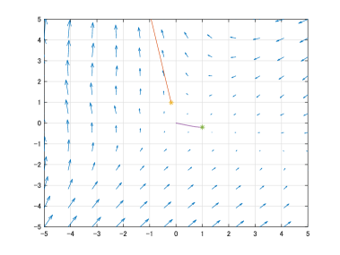
Figure 5: State trajectories from the initial conditions $\displaystyle x(0)=h_{1}$ and $\displaystyle x(0)=[\ 1\ -0.2\ ]^{T}$.

7 Conclusion

In this paper, we dealt with the stability analysis problem of feedback systems with ReLU nonlinearities. We particularly focused on the semialgebraic set representation that accurately characterizes the input-output properties of ReLUs. On the basis of this semialgebraic set representation, we derived a primal LMI for the stability certificate, and further derived a dual LMI for the instability certificate. In addition, we constructed a hierarchy of dual LMIs with which the detection of the instability is more likely to be expected. It is our important future topic to analyze the asymptotic behavior of this hierarchy of dual LMIs.

References

- Carrasco et al. (2016) Carrasco, J., Turner, M., and Heath, W. (2016). Zames–Falb multipliers for absolute stability: From O’shea’s contribution to convex searches. European Journal of Control, 28, 1–19.
- Dür (2010) Dür, M. (2010). Copositive programming - a survey. In M. Diehl, F. Glineur, E. Jarlebring, and W. Michiels (eds.), Recent Advances in Optimization and Its Applications in Engineering, 3–20. Springer.
- Ebihara (2012) Ebihara, Y. (2012). Systems Control Using LMI (in Japanese). Morikita Syuppan Co., Ltd, Tokyo.
- Ebihara et al. (2009) Ebihara, Y., Onishi, Y., and Hagiwara, T. (2009). Robust performance analysis of uncertain LTI systems: Dual LMI approach and verifications for exactness. IEEE Transactions on Automatic Control, 54(5), 938–951.
- Ebihara et al. (2021) Ebihara, Y., Waki, H., Magron, V., Mai, N.H.A., Peaucelle, D., and Tarbouriech, S. (2021). induced norm analysis of discrete-time LTI systems for nonnegative input signals and its application to stability analysis of recurrent neural networks. The 2021 ECC Special Issue of the European Journal of Control, 62, 99–104.
- Ebihara et al. (2024) Ebihara, Y., Xin, D., Magron, V., Peaucelle, D., and Tarbouriech, S. (2024). Local Lipschitz constant computation of ReLU-FNNs: Upper bound computation with exactness verification. In arxiv:2310.11104 in math.OC, also to appear in Proc. the 22nd European Control Conference.
- Fazlyab et al. (2022) Fazlyab, M., Morari, M., and Pappas, G.J. (2022). Safety verification and robustness analysis of neural networks via quadratic constraints and semidefinite programming. IEEE Transactions on Automatic Control, 67(1), 1–15.
- Fetzer and Scherer (2017) Fetzer, M. and Scherer, C.W. (2017). Absolute stability analysis of discrete time feedback interconnections. IFAC PapersOnline, 50(1), 8447–8453.
- Groff et al. (2019) Groff, L.B., Valmorbida, G., and da Silva, J.M.G. (2019). Stability analysis of piecewise affine discrete-time systems. In Proc. Conference on Decision and Control, 8172–8177.
- Grönqvist and Rantzer (2022) Grönqvist, J. and Rantzer, A. (2022). Dissipativity in analysis of neural networks. In Proc. the 25th International Symposium on Mathematical Theory of Networks and Systems, 1221–1224.
- Henrion and Lasserre (2005) Henrion, D. and Lasserre, J.B. (2005). Detecting global optimality and extracting solutions in gloptipoly. In D. Henrion and A. Garulli (eds.), Lecture Notes in Control and Information Sciences, volume 312. Springer Verlag, Berlin.
- Khalil (2002) Khalil, H. (2002). Nonlinear Systems. Prentice Hall.
- Lasserre (2001) Lasserre, J.B. (2001). Global optimization with polynomials and the problem of moments. SIAM Journal on Optimization, 11(3), 796––817.
- Magron and Wang (2023) Magron, V. and Wang, J. (2023). Sparse Polynomial Optimization: Theory and Practice. World Scientific.
- Masubuchi and Scherer (2009) Masubuchi, I. and Scherer, C.W. (2009). A recursive algorithm of exactness verification of relaxations for robust SDPs. Systems and Control Letters, 58(8), 592–601.
- Megretski and Rantzer (1997) Megretski, A. and Rantzer, A. (1997). System analysis via integral quadratic constraints. IEEE Transactions on Automatic Control, 42(6), 819–830.
- O’Shea (1967) O’Shea, R. (1967). An improved frequency time domain stability criterion for autonomous continuous systems. IEEE Transactions on Automatic Control, 12(6), 725–731.
- Raghunathan et al. (2018) Raghunathan, A., Steinhardt, J., and Liang, P. (2018). Semidefinite relaxations for certifying robustness to adversarial examples. Advances in Neural Information Processing Systems, 10900–10910.
- Revay et al. (2021) Revay, M., Wang, R., and Manchester, I.R. (2021). A convex parameterization of robust recurrent neural networks. IEEE Control Systems Letters, 5(4), 1363–1368.
- Scherer (2005) Scherer, C.W. (2005). Relaxations for robust linear matrix inequality problems with verifications for exactness. SIAM Journal on Matrix Analysis and Applications, 27(2), 365–395.
- Scherer (2006) Scherer, C.W. (2006). LMI relaxations in robust control. European Journal of Control, 12(1), 3–29.
- Scherer (2022) Scherer, C.W. (2022). Dissipativity and integral quadratic constraints: Tailored computational robustness tests for complex interconnections. IEEE Control Systems Magazine, 42(3), 115–139.
- Tarbouriech et al. (2011) Tarbouriech, S., Garcia, G., Jr., G.S., and Queinnec, I. (2011). Stability and Stabilization of Linear Systems with Saturating Actuators. Springer.
- Yin et al. (2022) Yin, H., Seiler, P., and Arcak, M. (2022). Stability analysis using quadratic constraints for systems with neural network controllers. IEEE Transactions on Automatic Control, 67(4), 1980–1987.
- Zames and Falb (1968) Zames, G. and Falb, P. (1968). Stability conditions for systems with monotone and slope-restricted nonlinearities. SIAM Journal on Control, 6(1), 89–108.
- Zhang (2020) Zhang, R.Y. (2020). On the tightness of semidefinite relaxations for certifying robustness to adversarial examples. Advances in Neural Information Processing Systems, 33, 3808–3820.