The Maslov index, degenerate crossings and the stability of pulse solutions to the Swift-Hohenberg equation

Abstract

In the scalar Swift-Hohenberg equation with quadratic-cubic nonlinearity, it is known that symmetric pulse solutions exist for certain parameter regions. In this paper we develop a method to determine the spectral stability of these solutions. We first associate a Maslov index to each solution and then argue that this index coincides with the number of unstable eigenvalues for the linearized evolution equation. This requires extending the method of computing the Maslov index introduced by Robbin and Salamon to so-called degenerate crossings. We extend their formulation of the Maslov index to degenerate crossings of general order. Furthermore, we develop a numerical method to compute the Maslov index associated to symmetric pulse solutions. Finally, we consider several solutions to the Swift-Hohenberg equation and use our method to characterize their stability.

1 Introduction

Coherent structures, such as wave trains, fronts and pulses, often occur in spatiotemporal systems found in nature or laboratory settings.. Mathematically, these objects can be studied as the solutions of partial differential equations posed on infinite domains. Oftentimes, one wants to understand the long term behavior of these models to gain insight into observable physical phenomena. To understand the long term behavior of these models, one often begins by seeking to understand the stability of these coherent structures. One can study spectral, linear and nonlinear (in)stabilities of such solutions. In particular, spectral stability is determined by whether the linearization of the PDE about a given solution has spectrum with positive real part. The spectrum can be divided into two disjoint sets: the essential and point spectrum. The essential spectrum is often relatively easy to compute, so the bulk of the work in determining spectral stability lies in looking for unstable eigenvalues.

This work seeks to understand the (in)stability of pulse solutions to the Swift-Hohenberg equation. The Swift-Hohenberg equation [CH93, HS77] for $u:\mathbb{R}\times\mathbb{R}^{+}\to\mathbb{R}$ is defined as

$$u_{t}=-(1+\partial_{x}^{2})^{2}u+f(u),$$ (1.1)

where the nonlinearity $f$ is typically chosen to be a parameter-dependent polynomial. For real parameters $\mu$ and $\nu$, we will work with the nonlinearity

$$f(u)=\nu u^{2}-u^{3}-\mu u.$$ (1.2)

This equation was derived by Swift and Hohenberg in 1977 to study thermal fluctuations of a fluid near the Rayleigh-Benard convective instability, but has since been used as a general model with which to study pattern-forming behavior. For the Swift-Hohenberg equation, spectral stability is necessary for both linear and nonlinear stability [Hen81]. Therefore, if we can show that a pulse solution is spectrally unstable, then it is linearly and nonlinearly unstable as well.

Previous work has addressed the existence of pulse solutions to the 1D Swift-Hohenberg equation using numerical methods [BK07a, BK07c, BK07b] and spectral methods have been used to compute the eigenvalues of these solutions [BK06] for certain parameter regimes. The work of [MS19, BKL⁺09a] rigorously proved that a pulse solution can be formed by concatenating front and back solutions. Furthermore, the work of [MS19] argues that these pulse solutions are stable if and only if the front and back solutions are stable.

We seek to round out this theory by providing a framework that can be used to count the eigenvalues of these pulse solutions. This framework is general in the sense that it can be used to characterize both spectral stability and spectral instability of such solutions. Additionally, this framework applies to a wide range of parameter values (see Hypothesis 1.2). Furthermore, this paper lays the groundwork for our forthcoming paper that uses validated numerics to provide a mathematical proof of both the existence and stability of these pulse solutions.

Our strategy for proving the (in)stability of pulse solutions to the Swift-Hohenberg equation relies on the Maslov index. We will detect instabilities in the point spectrum by building directly on the results in [BCJ⁺18], which allow one to count unstable eigenvalues by instead counting objects referred to as conjugate points. This extension is nontrivial due to the presence of nonregular (degenerate) crossings, which we will say more about shortly. In order to address this degeneracy, we will generalize the crossing form and main results of [RS93] so that they apply to degenerate crossings of any order. We will describe how our contribution to Maslov theory fits within the existing body of work in Section 1.1. Lastly, we numerically compute conjugate points and estimate unstable eigenvalues for several example pulse solutions using Fourier methods as a proof of concept.

For an open parameter region, the Swift-Hohenberg equation admits symmetric pulse solutions. In particular, for certain parameter values, one can observe interesting behavior called homoclinic snaking in which there are an infinite number of symmetric (and asymmetric) pulse solutions [BKL⁺09a]. We will look at two sets parameter values. The parameter values $(\nu,\mu)=(1.6,0.05)$ lie outside of the snaking region and for these parameter values there are two symmetric pulse solutions. We also consider the parameter values $(\nu,\mu)=(1.6,0.20)$ lie within the snaking region. The branches of symmetric pulse solutions are given by (4.1) and setting $\phi=0,\pi$. We denote each pulse solution as $\varphi_{\phi}(x;\nu,\mu)$ so we can specify the corresponding phase condition $\phi$ in (4.1) and the parameter values $\nu$ and $\mu$. Example parameter values and solutions are depicted in Figure 1. The numbers of unstable eigenvalues for the example solutions in Figure 1 are given in Table 1.

Symmetric Pulse	# Unstable Eigenvalues	# Conjugate Points
$\varphi_{\phi}(x;\nu,\mu)$
$\varphi_{0}(x;1.6,0.05)$	1	1
$\varphi_{\pi}(x;1.6,0.05)$	2	2
$\varphi_{0}(x;1.6,0.2)$	None	None

Table 1: Number of unstable eigenvalues and conjugate points for the example symmetric pulse solutions.

(a) $\varphi_{0}(x;1.6,0.05)$

(b) $\varphi_{\pi}(x;1.6,0.05)$

(c) $\varphi_{0}(x;1.6,0.2)$

Figure 1: Example symmetric pulse profiles.

In order to say more about the works we will build on [BCJ⁺18, BJ22] and to describe our results in more detail, we now introduce some assumptions and basic facts about our setting. We will also introduce relevant terminology concerning the Maslov index and the Lagrangian Grassmannian.

1.1 Mathematical Preliminaries

When studying the spectral stability of a solution $\varphi$ to a PDE, one begins by linearizing about $\varphi$ to form a differential operator $\mathcal{L}$. The spectral stability of $\varphi$ is determined by the spectrum of this differential operator. If $\mathcal{L}$ has domain $D$, the point spectrum of $\mathcal{L}$ satisfies the eigenvalue problem

$$\mathcal{L}u=\lambda u,\qquad u\in D.$$ (1.3)

In our context, the first order system corresponding to (1.3) will be given by a first order Hamiltonian system of the form

$$q^{\prime}=JC(x,\lambda)q,\qquad\qquad q\in\mathbb{R}^{2n},\ J=\begin{pmatrix}0&I_{n}\\ -I_{n}&0\end{pmatrix},$$ (1.4)

where $C(x,\lambda)$ is a $2n\times 2n$ symmetric matrix. Define the stable and unstable subspaces of solutions to (1.4) as

$$\begin{split}\mathbb{E}^{s}_{+}(x,\lambda)&:=\bigg{\{}u\in\mathbb{R}^{2n}\ :\ u\text{ solves }\eqref{eq: general Hamiltonian}\text{ and }\lim_{x\to\infty}\|u(x,\lambda)\|\to 0\bigg{\}}\\ \mathbb{E}^{u}_{-}(x,\lambda)&:=\bigg{\{}u\in\mathbb{R}^{2n}\ :\ u\text{ solves }\eqref{eq: general Hamiltonian}\text{ and }\lim_{x\to-\infty}\|u(x,\lambda)\|\to 0\bigg{\}}.\end{split}$$ (1.5)

We will consider the evolution of $\mathbb{E}^{u}_{-}(x,\lambda)$ as either $x$ or $\lambda$ varies. More generally, both of these subspaces of solutions have a symplectic structure. To see why, let $u,v$ be solutions of (1.4) and observe

$$\frac{d}{dx}\langle u,Jv\rangle=\langle u^{\prime},Jv\rangle+\langle u,Jv^{\prime}\rangle=\langle JCu,Jv\rangle+\langle u,JJCv\rangle=\langle u,C^{T}v\rangle-\langle u,Cv\rangle=0;$$

where we have used that $C$ is symmetric and $J^{T}=-J=J^{-1}$. We now introduce the terminology and background necessary for further study of these subspaces through the lens of symplectic geometry.

Given any $d$-dimensional vector space $V$, $G_{k}(V)$ denotes the set of all $k$-dimensional linear subspaces of $V$. When this set is given the structure of a smooth manifold, it is called the Grassmannian manifold. A symplectic form $\omega$ on $V$ is an anti-symmetric non-degenerate bilinear form on $V$ and taken together, the pair $(V,\omega)$ is called a symplectic vector space. If $V$ is finite dimensional, its dimension must be even. Thus, let $d=2n$ and consider $G_{n}(\mathbb{R}^{2n})$. A Lagrangian plane is an $n$-dimensional subspace $\ell\in G_{n}(\mathbb{R}^{2n})$ with the property that $\omega(u,v)=0$ for all vectors $u,v\in\ell$. The collection of all Lagrangian planes is called the Lagrangian Grassmannian and denoted by $\Lambda(n)$. In principle, the structure of $\Lambda(n)$ depends on the choice of $\omega$, but one can show the resulting spaces all have the same topological properties. We will be concerned only with the symplectic form defined by

$$\omega(u,v)=\langle u,Jv\rangle,\qquad J=\begin{pmatrix}0&I_{n}\\ -I_{n}&0\end{pmatrix},$$ (1.6)

where $\langle\cdot,\cdot\rangle$ denotes the usual inner product on $\mathbb{R}^{2n}$.

When referring to elements of $\Lambda(n)$, we will use the notation $\ell\in\Lambda(n)$ or another calligraphic letter. It will also be convenient to refer to a Lagrangian plane using a particular choice of a frame matrix. This means choosing $n\times n$ real matrices $X$ and $Y$ so that

$$\ell=\left\{\begin{pmatrix}X\\ Y\end{pmatrix}u:u\in\mathbb{R}^{n}\right\}.$$ (1.7)

To denote the frame matrix we will typically use block letters and write $L=\begin{pmatrix}X&Y\end{pmatrix}^{T}$ inline or

$$L=\begin{pmatrix}X\\ Y\end{pmatrix}.$$

The choice of frame matrix is not unique. If $M$ is any invertible $n\times n$ real matrix, then $\begin{pmatrix}XM&YM\end{pmatrix}^{T}$ is also a frame matrix for the same Lagrangian plane. One can check that an $n$-dimensional subspace defined via (1.7) is Lagrangian if and only if $X^{T}Y=Y^{T}X$ and the column rank of $\begin{pmatrix}X&Y\end{pmatrix}^{T}$ is $n$. We will be particularly interested in paths of Lagrangian planes on a compact domain, which we will denote by $\ell(t)$, or by its frame matrix $L(t)$, or via the component block matrices $X(t)$ and $Y(t)$ for $t$ in some interval.

This framework is particularly useful for the study of first-order Hamiltonian eigenvalue problems like (1.4), because the associated stable and unstable subspaces in (1.5) are paths of Lagrangian planes.

We now describe how to leverage this framework to study solutions to (1.3). One has an eigenvalue of $\mathcal{L}$ at $\lambda=\lambda_{*}$ if there exists a solution to (1.4) that decays to zero as $|x|\to\infty$. Note that one really needs the solution to live in an appropriate Banach space but for most spaces, if one assumes that the essential spectrum is bounded away from $0$, this is equivalent to asymptotic decay of the eigenfunction. This directly corresponds to a nontrivial intersection of the stable and unstable subspaces for that value of the spectral parameter: $\mathbb{E}^{u}_{-}(x;\lambda_{*})\cap\mathbb{E}^{s}_{+}(x;\lambda_{*})\neq\{0\}$. The operator $\mathcal{L}$ has real spectrum since it is self adjoint so one could detect unstable eigenvalues by asking, are there any values of $\lambda>0$ such that $\mathbb{E}^{u}_{-}(x;\lambda)\cap\mathbb{E}^{s}_{+}(x;\lambda)\neq\{0\}$?

It is perhaps surprising that one can reformulate this question as follows. Pick any fixed Lagrangian plane $\ell_{*}\in\Lambda(n)$, which we will call the reference plane. Fix the spectral parameter to be $\lambda=0$ and ask, are there any values of $x\in\mathbb{R}$ for which $\mathbb{E}^{u}_{-}(x;0)\cap\ell_{*}\neq\{0\}$? Values $x=x_{0}$ where $\mathbb{E}^{u}_{-}(x_{0};0)\cap\ell_{*}\neq\{0\}$ are called conjugate points. This reformulation amounts to saying that the number of unstable eigenvalues of $\mathcal{L}$ is equal to the number of conjugate points associated with the reference plane $\ell_{*}$ at $\lambda=0$ and it can be understood via the use of the Maslov index. The main results of this paper are justifying this reformulation in the context of the Swift-Hohenberg equation and providing a framework for counting the conjugate points.

The Maslov index is used in the study of symplectic geometry and the theory of Fredholm operators. It is a counting index that provides a measure of the number of times a certain type of curve, called a Lagrangian submanifold, intersects a given surface in a symplectic space. This count can be used to provide a topological characterization of solutions to Hamiltonian systems that determines their spectral stability.

The main properties of the intersection number of Lagrangian submanifolds were proven in [Arn67] and followed by results that connect the Maslov index to self-adjoint operators [Arn85, Dui76]. These results can be viewed as generalizations of classical Sturm Liouville theory [Sma65, Bot56, Edw64]. Beginning with Jones’ work [Jon88], the Maslov index has been used as a tool to study stability in systems that are Hamiltonian in their spatial variables [CJM17, CJM15, HS16, HLS18, CJLS16]. While these results connect the number of unstable eigenvalues to the number of conjugate points, it is often unclear how to find the number of conjugate points, which is necessary for this framework to be useful in determining spectral stability. There are two examples of systems for which the number of conjugate points has been computed for specific solutions, the first is [BCJ⁺18], in which the Maslov index was used to show that a symmetric pulse solution to a system of reaction diffusion equations is unstable. This was followed by [BJ22], in which the Maslov index and computer assisted proofs were used to argue that a parameter dependent system of bistable equations has both stable and unstable fronts.

Our goal is to use the Maslov index to argue that a pulse solution to the Swift-Hohenberg equation is unstable in certain parameter regions. In order to do so, we further Maslov theory in two distinct directions. In the first direction, we apply the Maslov index to a fourth order system that has not been considered in previous literature. We note that the unstable eigenvalues of certain fourth-order potential systems can be counted using the Maslov index [How21b], but the Swift-Hohenberg equation falls outside the class of considered operators. The second contribution that this work makes is the generalization of the crossing form introduced in [RS93] to $k$th order degenerate crossings. Previous results rely on so-called regular crossings, with two notable exceptions [DJ11, CCLM23], in which second order crossings are considered. Since the Swift-Hohenberg equation has third order crossings, these results do not apply and our theory is not restricted to a particular order of crossing. Furthermore, we discuss a previously unaddressed subtlety concerning the formulation of Lagrangian planes as graphs that becomes critical in calculations for non-regular crossings.

We begin by stating some assumptions and basic facts about this setting, which will enable us to then explain our main results. First, we assume that the nonlinearity $f(u)$ supports the existence of a pulse solution.

Hypothesis 1.1.

There exists a stationary solution $\varphi$ to (1.1) such that $\lim_{x\to\pm\infty}\varphi(x)=0$.

Linearizing about a stationary solution $\varphi$ and formulating the associated eigenvalue problem yields

$$\begin{split}\mathcal{L}u&=\lambda u,\\ \mathcal{L}=-\partial_{x}^{4}-2&\partial_{x}^{2}-1+f^{\prime}\circ\varphi(x).\end{split}$$ (1.8)

We are primarily interested in detecting spectral instabilities, which means determining whether or not the spectrum of $\mathcal{L}$ has positive real part. Since the spectrum can be divided into the essential spectrum and point spectrum, and the essential spectrum is typically easy to compute, we wish to assume the essential spectrum is stable and focus on detecting instabilities in the point spectrum. Therefore, we make the following second assumption, which implies that the essential spectrum of the pulse is contained in the open left half plane [KP13].

Hypothesis 1.2.

The derivative of the nonlinearity $f(u)$ in (1.1) evaluated at $u=0$ is negative.

Remark 1.3.

This hypothesis is necessary for the essential spectrum of $\mathcal{L}$ to be negative. It is important that the essential spectrum is negative instead of just nonositive, because our analysis for $\lambda\in[0,\infty)$ relies on the existence of exponential dichotomies on $\mathbb{R}^{+}$ and $\mathbb{R}^{-}$ [Cop78].

To detect unstable eigenvalues, we will exploit the symplectic structure of the eigenvalue equation (1.8), which can be seen via the change of variables

$$q_{1}=u,\qquad q_{2}=u_{xx},\quad q_{3}=u_{xxx}+2u_{x},\quad q_{4}=u_{x}.$$ (1.9)

This allows us to write (1.8) as the first order system

$$\begin{split}q^{\prime}&=B(x,\lambda)q,\qquad B(x,\lambda):=\begin{pmatrix}0&0&0&1\\ 0&0&1&-2\\ -\lambda-1+f^{\prime}\circ\varphi(x)&0&0&0\\ 0&1&0&0\end{pmatrix}.\end{split}$$ (1.10)

Since this system is Hamiltonian, we can also formulate the above equation as

$$\begin{split}q^{\prime}&=JC(x,\lambda)q,\\ J=\begin{pmatrix}0&I_{2}\\ -I_{2}&0\end{pmatrix},&\qquad C(x,\lambda)=\begin{pmatrix}\lambda+1-f^{\prime}\circ\varphi(x)&0&0&0\\ 0&-1&0&0\\ 0&0&0&1\\ 0&0&1&-2\end{pmatrix}.\end{split}$$ (1.11)

Note that we can also express this as $q^{\prime}=-J\nabla_{q}H(x,q)$, where

$$H(x,q)=\frac{1}{2}\big{(}-\lambda-1+f^{\prime}\circ\varphi(x)\big{)}q_{1}^{2}+\frac{1}{2}q_{2}^{2}-q_{3}q_{4}+q_{4}^{2}.$$ (1.12)

Remark 1.4.

If a solution $q(x;\lambda)$ lies in $\mathbb{E}^{u}_{-}(x;\lambda)$, then $q$ lies in the $0$ energy level and $H(x,q)=0$.

Using Hypothesis 1.1, we find the asymptotic limits of the coefficient matrix $B$ in (1.10) to be given by

$$B_{\infty}(\lambda):=\lim_{x\to\pm\infty}B(x,\lambda)=\begin{pmatrix}0&0&0&1\\ 0&0&1&-2\\ -\lambda-1+f^{\prime}(0)&0&0&0\\ 0&1&0&0\end{pmatrix}.$$ (1.13)

The asymptotic matrix $B_{\infty}(\lambda)$ is useful in understanding the dynamics of (1.10) because it governs the asymptotic behavior of the system. We collect the relevant properties of $B_{\infty}(\lambda)$ into the below lemma.

Lemma 1.5.

Let $B_{\infty}$ be as defined in (1.13). Then

1. $B_{\infty}(\lambda)$ is hyperbolic for all $\lambda\geq 0$.

2. The matrix $B_{\infty}$ depends analytically on $\lambda$. Also, there are positive constants $K_{B}$ and $C_{B}$, independent of $\lambda$, such that

   $$\|B(x;\lambda)-B_{\infty}(\lambda)\|\leq K_{B}e^{-C_{B}|x|}\text{ as }x\to\pm\infty.$$ (1.14)

Proof.

See Section A.1.1. ∎

1.2 Statement of Main Results

We now state the main result of our work.

Theorem 1.6.

Let $\ell(x)=\mathbb{E}^{u}_{-}(x;0)$ and fix the reference plane $\ell_{*}=\ell^{sand}_{*}$ with

$$\ell^{sand}_{*}=\text{colspan}\begin{pmatrix}0&0\\ 1&0\\ 0&1\\ 0&0\end{pmatrix}.$$

The number of unstable eigenvalues of the operator in (1.8) acting on $H^{4}(\mathbb{R})$ is equal to the number of conjugate points of the path $\ell(x)$ with respect to the reference plane $\ell_{*}^{sand}$.

Remark 1.7.

The notation $\ell_{*}^{sand}$ is chosen because the identity matrix is “sandwiched” between two rows of zeros. This choice of reference plane is used to study fourth-order potential systems in [How21a, How21b].

The remainder of the paper is organized as follows. We establish further background in §2 on the Lagrangian Grassmannian and related objects, which are necessary to provide a precise definition of conjugate points. We also provide a formulation of the Maslov index that applies to degenerate crossings and generalize the results of [RS93]. In §3 we prove Theorem 1.6 and compute the conjugate points in §4 using numerics. In §5 we discuss future work and in the appendix §A we discuss an explicit example and collect some technical results about coordinate changes and representing subspaces as a graph.

2 Conjugate Points and the Crossing Form

In this section we establish further background on conjugate points and the crossing form. Recall that we are interested in detecting eigenvalues of (1.8) by finding objects called conjugate points. Conjugate points occur when the path of Lagrangian subspaces given by $\mathbb{E}^{u}_{-}(x,\lambda)$ intersect a fixed reference plane. These intersections are detected with a quadratic form called the crossing form that was developed in [RS93] and the sign of this quadratic form determines the sign with which the conjugate points contribute to the Maslov index. Intuitively, the crossing form is performing a first derivative test on a particular function and if the function is increasing, then the crossing form is positive and the crossing contributes to the Maslov index with positive sign (similarly for the decreasing/negative case).

As an example, consider the function $f(t)=\pm t^{j}$ and suppose that we are interested in whether $f$ is increasing or decreasing at $t=0$. If $f(t)$ is linear, then the first derivative will give us this information. This first derivative test is the analogue of the crossing form developed in [RS93]. However, if $f$ is a higher order polynomial, then the first derivative at $t=0$ vanishes and we must use a higher order derivative test by finding the lowest $j\in\mathbb{N}$ such that $\frac{d^{j}}{dt^{j}}f(t)\big{|}_{t=0}=f^{(j)}(0)\neq 0$.

(a) $j$ even

(b) $j$ odd

Figure 2: The function $f(t)=\pm t^{j}$ near $t=0$. The case that $f^{(j)}(0)>0$ is depicted by the dashed line and the case that $f^{(j)}(0)<0$ is given by the solid line.

In the case of the Swift-Hohenberg equation, we will need to use the equivalent of a third order derivative test to determine the sign of the contribution to the Maslov index. The goal of this section is to develop the analogue of a higher order derivative test via higher order crossing forms for the Maslov index. Compare Figure 2 depicting $f(t)$ with Figure 6 depicting the information given by the higher order crossing forms.

To this end, we first discuss the formulation of a path of Lagrangian planes as the graph of a matrix. We will then see in subsequent sections that the Maslov index can be connected to the eigenvalues of this matrix. There are several subtleties associated with the graph formulation of a Lagrangian subspace that are critical in the computation of higher order crossing forms (see Remark 3.12).

Let $\ell(t)$ be a Lagrangian path defined for $t\in[a,b]$ with frame matrix $L(t)$. Fix $t_{0}\in[a,b]$ and let $\mathcal{W}$ be a Lagrangian plane such that $\ell(t_{0})\cap\mathcal{W}=\{0\}$. Then, there exists an $\epsilon>0$ and a $2n\times 2n$ matrix $A(t):\ell(t_{0})\to\mathcal{W}$ such that for all $v\in\ell(t_{0})$, we have $v\in\ker A(t_{0})$ and

$$v+A(t)v\in\ell(t),\qquad\ t\in(t_{0}-\epsilon,t_{0}+\epsilon).$$ (2.1)

Figure 3: Representing $\ell(t)$ as a graph for $t$ near $t_{0}$.

In particular, suppose we are given a Lagrangian subspace $\ell(t)$ with frame

$$L(t)=\begin{pmatrix}|&&|\\ v_{1}(t)&\dots&v_{n}(t)\\ |&&|\end{pmatrix}.$$

For $i=1,\dots,n$, fix $k_{i}\in\mathbb{R}$, and define $v=\sum_{i=1}^{n}k_{i}v_{i}(t_{0})\in\ell(t_{0})$. Then, there is a matrix $A(t):\ell(t_{0})\to\mathcal{W}$ and functions $c_{i}(t):\mathbb{R}\to\mathbb{R}$, such that for all $v\in\ker A(t_{0})$ and $t\in(t_{0}-\epsilon,t_{0}+\epsilon)$,

$$\begin{split}v+A(t)v\ &=\sum_{i=1}^{n}c_{i}(t)v_{i}(t),\\ &=L(t)c(t),\qquad c(t):=\big{(}c_{1}(t),\dots,c_{n}(t)\big{)}^{T}.\\ \end{split}$$ (2.2)

The coefficient functions $c_{i}(t)$ may depend on $t$ and the constant coefficients $k_{i}$ that determine $v$. See Section A.2 for an explicit example.

2.1 The Crossing Form and the Maslov Index

We now introduce the terminology and framework developed in [RS93] to understand the evolution of the Lagrangian subspace $\ell(t)$ with respect to another fixed Lagrangian plane.

Definition 2.1.

[RS93] Suppose that $\ell(t)$ is a smooth path of Lagrangian planes in $\mathbb{R}^{2n}$. Fix $t_{0}$ and choose $\mathcal{W}$ such that $\mathcal{W}\cap\ell(t_{0})=\{0\}$. For $v\in\ell(t_{0})$ and $t$ near $t_{0}$ define the operator $A(t):\ell(t_{0})\to\mathcal{W}$ such that its graph is $\ell(t)$. In particular, for all $v\in\ell(t_{0})$, we have $v+A(t)v\in\ell(t)$. Then, the first order quadratic form associated with $\ell(t)$ at $t=t_{0}$ acting on the vector $v$ is defined as

$$Q^{(1)}(v)=\frac{d}{dt}\omega(v,A(t)v)\bigg{|}_{t=t_{0}}.$$ (2.3)

The following result from [RS93] concerns the first order quadratic form.

Theorem 2.2.

[RS93][Theorem 1.1] Let $\ell(t)\in\Lambda(n)$ be a $C^{1}$ path of Lagrangian planes with frame $L(t)=\begin{pmatrix}X(t)&Y(t)\end{pmatrix}$. For fixed $t_{0}$ and $v\in\ell(t_{0})$, let $Q^{(1)}(v)$ be as in Definition 2.1.

1. The first order quadratic form is invariant under symplectic changes of coordinates.

2. The first order quadratic form is independent of the choice of plane $\mathcal{W}$.

3. Let $v=L(t_{0})u$ with $v\in\mathbb{R}^{2n}$ and $u\in\mathbb{R}^{n}$. Then $Q^{(1)}(v)$ can be calculated via the formula

   $$Q^{(1)}(v)=\big{\langle}X(t_{0})u,\dot{Y}(t_{0})u\big{\rangle}-\big{\langle}Y(t_{0})u,\dot{X}(t_{0})u\big{\rangle}.$$

Remark 2.3.

We refer the reader to [MS17][Chapter 2] for a review of symplectic coordinates. For this work, it is sufficient to recall that a $2n\times 2n$ matrix $\Psi$ is symplectic if $\Psi^{T}J\Psi=J$ and that a symplectic change of coordinates is done via a symplectic transition matrix.

Fix a subspace $\ell_{*}$ such that $\ell_{*}\cap\ell(t_{0})\neq\{0\}$. If we restrict the first order quadratic form to $v\in\ell(t_{0})\cap\ell_{*}$, then we obtain the first order crossing form. Before giving this definition, we first formalize the notion of a crossing.

Definition 2.4.

[Arn67] A crossing for the path $\ell(t)\in\Lambda(n)$ with respect to a fixed $\ell_{*}$ is a value $t_{0}\in[a,b]$ such that $\ell(t_{0})\cap\ell_{*}\neq\{0\}.$ The plane $\ell_{*}$ is often called a reference plane. We use the following terminology to describe crossings:

1. a crossing is simple if $\ell(t_{0})\cap\ell_{*}$ is a one dimensional subspace of $\mathbb{R}^{2n}$;

2. a crossing is isolated if there exists $\epsilon>0$ such that $\ell(t)\cap\ell_{*}=\{0\}$ for all $t\in[t_{0}-\epsilon,t_{0}+\epsilon]\setminus\{t_{0}\}$.

Now we are in a position to define the crossing form and associated terminology.

Definition 2.5.

[RS93] The first order crossing form with respect to $\ell(t)$ and $\ell_{*}$ is defined to be the first order quadratic form restricted to $\ell(t_{0})\cap\ell_{*}$:

$$\Gamma(\ell,\ell_{*},t_{0}):=Q^{(1)}(v),\qquad v\in\ell(t_{0})\cap\mathcal{\ell}_{*}.$$ (2.4)

We say a crossing $t_{0}$ is regular or non-degenerate if the crossing form $\Gamma$ is non-singular.

Our notation for this quadratic form differs slightly from that in [RS93] due to the addition of the superscript in $Q^{(1)}$. We introduce this extra notation to denote the first derivative contained in this quadratic form. This will be useful later in Section 2.2 when we take higher order derivatives to construct higher order quadratic forms. The crossing form can be used to explore the signed intersections of $\ell(t)$ with a reference plane, $\mathcal{\ell}_{*}$. If $\Pi$ denotes the projection operator onto $\ell_{*}\cap\ell(t_{0})$, then the matrix that determines $Q^{(1)}(v)$ is $\Pi J\dot{A}(t_{0})\Pi$; this follows from Definition 2.5 and the restriction of $v\in\ell(t_{0})\cal\ell_{*}$. Proposition A.2 says this matrix is symmetric so all of its eigenvalues are real.

The signature of a matrix $B$ is defined as $\text{sign}B=p-q$ where $p$ is the number of positive eigenvalues and $q$ is the number of negative eigenvalues of $B$. We define the signature of a quadratic form as the signature of the matrix that determines the quadratic form. For this reason, we write $\text{sign}Q^{(1)}$ and do not specify the argument because this signature does not depend on the argument $v$.

Definition 2.6.

[RS93, Dui76] Following the setting and notation of Definitions 2.1 and 2.5, define $\Gamma^{+}(\ell,\ell_{*},t)$ and $\Gamma^{-}(\ell,\ell_{*},t)$ to the be right and left derivatives of $\omega(v,A(t)v)$ respectively. For a smooth curve $\ell:[a,b]\to\Lambda(n)$ with only regular crossings, we define the Maslov index to be

$$\text{Mas}(\ell(t),\ell_{*};\ a\leq t\leq b)=\frac{1}{2}\text{sign }\Gamma^{+}(\ell,\ell_{*},a)+\sum_{a<t<b}\text{sign }\Gamma(\ell,\ell_{*},t)+\frac{1}{2}\text{sign }\Gamma^{-}(\ell,\ell_{*},b),$$

where the sum is taken over all crossings $t$.

The important features of the Maslov index for this work are given below:

Lemma 2.7.

[RS93] Suppose that $\ell:[a,b]\to\Lambda(n)$ is a smooth path of Lagrangian subspaces and $\ell_{*}$ is a fixed reference plane.

1. (Additivity) For $a<c<b$

   $$\text{Mas}\left(\ell(t),\ell_{*};\ a\leq t\leq b\right)=\text{Mas}\left(\ell(t),\ell_{*};\ a\leq t\leq c\right)+\text{Mas}\left(\ell(t),\ell_{*};\ c\leq t\leq b\right).$$

2. (Homotopy invariance) Two paths $\ell_{1},\ell_{2}:[a,b]\to\Lambda(n)$ with $\ell_{1}(a)=\ell_{2}(a)$ and $\ell_{1}(b)=\ell_{2}(b)$ are homotopic with fixed endpoints if and only if they have the same Maslov index with respect to a fixed reference plane $\ell_{*}$.

We now discuss a formulation of the Maslov index from a spectral flow perspective. This formulation will be useful in the extension of the crossing form to non-regular crossings because it yields a definition of the Maslov index that does not rely on the non-degeneracy of the first order crossing form. Suppose that $\dim(\ell(t_{0})\cap\ell_{*})=k$. Then the matrix $\Pi JA(t_{0})\Pi$ has a $k$-dimensional kernel and the signature of the matrix $\Pi J\dot{A}(t_{0})\Pi$ tracks how many positive eigenvalues $\Pi JA(t)\Pi$ gains or loses as $t$ increases through $t_{0}$, which will be an integer in $\{-k,\dots,k\}$. Therefore, we can understand the contribution of a crossing to the Maslov index by studying the spectrum of $\Pi JA(t)\Pi$ for $t$ near $t_{0}$. We formalize this by following the work done in [Fur04]. We first have the following technical lemma.

Lemma 2.8.

[Fur04][Lemma 3.23] Fix $t_{0}$ and let $\{B(t)\}$ be a $C^{1}$ family of self-adjoint operators on $\mathbb{R}^{2n}$ for $t$ near $t_{0}$. Suppose that the set of $t$ for which $B(t)$ has a zero eigenvalue is comprised of singletons and that the quadratic form

$$R^{(1)}(x)=\frac{d}{dt}\langle x,B(t)x\rangle\bigg{|}_{t=t_{0}}=\left\langle x,\dot{B}(t_{0})x\right\rangle,\qquad x\in\ker B(t_{0})$$

is non-degenerate. Furthermore, suppose $\dim\ker B(t_{0})=k$. Then, there exists $p,q\in\mathbb{N}\cup\{0\}$ such that $p+q=k$ and $\epsilon,\delta>0$ such that $\text{sign}D^{(1)}=\text{sign}\dot{B}(t_{0})=p-q$. Furthermore,

1. for $t_{0}<t\leq t_{0}+\delta$, there are $p$ positive and $q$ negative eigenvalues of $B(t)$ within $\epsilon$ of $0$;

2. for $t_{0}-\delta\leq t<t_{0}$, there are $q$ positive eigenvalues and $p$ negative eigenvalues of $B(t)$ within $\epsilon$ of $0$.

Remark 2.9.

The condition that $\{t_{0}\ :\lambda(t_{0})=0\}$ in Lemma 2.8 is comprised of singletons is equivalent to the condition that the crossing at $t_{0}$ is isolated.

It is straightforward to relate Lemma 2.8 to the motion of the eigenvalues of $B(t)$ as $t$ increases through $0$.

Corollary 2.10.

Suppose we are in the setting of Lemma 2.8. If $\text{sign }R^{(1)}=p-q>0$, then the sign of the matrix $B(t)$ increases by $p-q$ as $t$ increases through $0$. If $\text{sign }R^{(1)}=p-q<0$, then the sign of $B(t)$ decreases by $p-q$ as $t$ increases through $0$.

Suppose the graph of $A(t):\ell(t_{0})\to\mathcal{W}$ is $\ell(t)$ for $t$ near $t_{0}$ and define $B(t)=JA(t)$ restricted to $\ell(t_{0})\cap\ell_{*}$. Recall that the projection operator onto $\ell(t_{0})\cap\ell_{*}$ is given by $\Pi$. Then via Corollary 2.10, the sign of the crossing form at a crossing $t=t_{0}$ satisfies

$$\text{sign}\Gamma(\ell,\ell_{*},t_{0})=\text{sign}Q^{(1)}=\text{sign}\Pi J\dot{A}(t_{0})\Pi=p-q,$$

which is precisely the number of positive eigenvalues that $\Pi JA(t)\Pi$ gains or loses as $t$ passes through $t=t_{0}$. This result is captured in the localization property of the Maslov index. The below theorem allows us to define the Maslov index in terms of the eigenvalues of $A(t)$ for $t$ near $t_{0}$ instead of relying on the derivative $\dot{A}(t_{0})$.

Theorem 2.11.

[RS93][Theorem 2.3] Suppose that $t_{0}$ is an isolated crossing of $\ell(t):[a,b]\to\Lambda(n)$ with reference plane $\ell_{*}$. Then if $t_{0}\in(a,b)$, we have for sufficiently small $\epsilon$, the Maslov index of $\ell:[t_{0}-\epsilon,t_{0}+\epsilon]\to\Lambda(n)$ is given by the spectral flow formulation

$$\text{Mas}(\ell,\ell_{*};|t-t_{0}|\leq\epsilon)=\frac{1}{2}\text{sign}\Pi JA(t_{0}+\epsilon)\Pi-\frac{1}{2}\text{sign}\Pi JA(t_{0}-\epsilon)\Pi.$$

If $t_{0}$ is equal to $a$ or $b$, then

$$\text{Mas}(\ell,\ell_{*};\ t_{0}\leq t\leq t_{0}+\epsilon) =\frac{1}{2}\text{sign}\big{[}\Pi JA(t_{0}+\epsilon)\Pi\big{]}-\frac{1}{2}\text{sign}\big{[}\Pi JA(t_{0})\Pi\big{]}$$

$$\text{Mas}(\ell,\ell_{*};\ t_{0}-\epsilon\leq t\leq t_{0}) =\frac{1}{2}\text{sign}\big{[}\Pi JA(t_{0})\Pi\big{]}-\frac{1}{2}\text{sign}\big{[}\Pi JA(t_{0}-\epsilon)\Pi\big{]}.$$

Remark 2.12.

It is important to note that Theorem 2.11 does not rely on the non-degeneracy of the crossing form because there is no differentiation. This fact will be useful in the proof of Theorem 2.21 when we extend the definition of the Maslov index via crossing forms to degenerate crossings. Additionally, our formulation of Theorem 2.11 differs slightly from the formulation in [RS93]. This is because we choose to represent $\ell(t)$ as the graph of a $2n\times 2n$ matrix in the standard coordinates on $\mathbb{R}^{2n}$ instead of changing coordinates and representing $\ell(t)$ as the graph of an $n\times n$ matrix.

2.2 Extending the Crossing Form to Nonregular Crossings

The formulation of the Maslov index discussed in the previous section only applies to regular crossings with the critical exception of Theorem 2.11. We will show in Section 3 that the Swift-Hohenberg equation has non-regular crossings and as a result, the formulation of the Maslov index using the crossing form that was previously introduced does not apply. A framework for computing the Maslov index for paths with second-order degenerate crossings has been established in the infinite dimensional case in [DJ11]. As we will see in in Section 3, the Swift-Hohenberg equation has third order degenerate crossings so we cannot directly apply a finite dimensional version of this result. We modify the result in [DJ11] and extend the theory introduced in Section 2.1 to degenerate crossings of general order in the finite dimensional case by using techniques similar to those used in [Fur04].

Definition 2.13.

Suppose that $\ell:[a,b]\to\Lambda(n)$ is a $C^{m}$ curve of Lagrangian subspaces and choose $\mathcal{W}$ such that $\ell(t_{0})\cap\mathcal{W}=\{0\}$ for fixed $t_{0}\in[a,b]$. For $v\in\ell(t_{0})$ and $t$ near $t_{0}$ suppose the graph of $A(t):\ell(t_{0})\to\mathcal{W}$ is $\ell(t)$ and fix $j\leq m$. Then, the quadratic form of order $j$ associated with $\ell(t)$ at $t=t_{0}$ acting on $v$ is defined as

$$Q^{(j)}(v)=\frac{d^{j}}{dt^{j}}\omega(v,A(t)v)\bigg{|}_{t=t_{0}}.$$ (2.5)

Fix a Lagrangian plane $\ell_{*}$ and we suppose at $t_{0}$, $\ell(t_{0})\cap\ell_{*}\neq\{0\}$. Then, the crossing form of order $j$ with respect to $\ell(t)$ and $\ell_{*}$ is defined to be

$$\Gamma^{(j)}(\ell,\ell_{*},t_{0})=Q^{(j)}(v),\qquad v\in\ell(t_{0})\cap\ell_{*}.$$ (2.6)

Below we prove a generalization of parts a) and b) of Theorem 2.2 for degenerate crossings via a different approach than the one used in [RS93]. Refer to Remark 2.3 for a brief discussion of symplectic coordinates.

Theorem 2.14.

Suppose we are in the setting of Definition 2.13. The higher order crossing form of order $j$ is

1. invariant under symplectic changes of coordinates;

2. independent of the choice of $\mathcal{W}$.

Proof.

1. Suppose that $\ell(t)$ has frame given by $L(t)$ and fix $v\in\ell(t_{0})$. Let $\mathcal{W}$ and $A(t)$ be as in Definition 2.13. Additionally, let $\Psi$ be a symplectic matrix and define the following quantities

   $$v_{\Psi}=\Psi v,\qquad\mathcal{W}_{\Psi}=\text{colspan}\big{(}\Psi W\big{)},\qquad\ell_{\Psi}(t)=\text{colspan}\big{(}\Psi\ell(t)\big{)}.$$

   Via (2.2), we have that

   $$v+A(t)v=L(t)c(t).$$

   By left multiplying by $\Psi$ and recalling that $v=\Psi^{-1}v_{\Psi}$, we can write

   $$\Psi v+\Psi A(t)v=v_{\Psi}+\Psi A(t)\Psi^{-1}v_{\Psi}=\Psi L(t)c(t).$$

   Thus, the graph of the matrix $A_{\Psi}(t):=\Psi A(t)\Psi^{-1}$ is $\ell_{\Psi}(t)$.

   Define $Q_{\Psi}(v):=\omega(v_{\Psi},A_{\Psi}(t)v_{\Psi})$ and observe the following inner product computation:

   $$Q_{\Psi}(v) :=\omega(v_{\Psi},A_{\Psi}(t)v_{\Psi})$$

   $$=\langle v_{\Psi},JA_{\Psi}(t)v_{\Psi}\rangle$$

   $$=\langle\Psi v,JA_{\Psi}(t)\Psi v\rangle$$

   $$=\langle v,\Psi^{T}JA_{\Psi}(t)\Psi v\rangle$$

   $$=\langle v,J\Psi^{-1}A_{\Psi}(t)\Psi v\rangle$$

   $$=\langle v,JA(t)v\rangle,$$

   where we have used that $\Psi$ is a symplectic matrix, so $\Psi^{-1}=J^{-1}\Psi^{T}J$. Thus,

   $$Q_{\Psi}(v)=\langle v,J\Psi^{-1}A_{\Psi}\Psi v\rangle=\langle v,JA(t)v\rangle:=Q(v).$$

   Since this is true for $t$ near $t_{0}$, the derivatives of $Q_{\Psi}(v)$ and $Q(v)$ coincide and we see that the crossing forms are invariant under symplectic changes of coordinates.

2. By the previous claim and [MS17][Lemma 2.3.2], we can change coordinates and assume that $\ell(t_{0})=\text{col span}\begin{pmatrix}I_{n}&0\end{pmatrix}^{T}$ and $\mathcal{W}=\text{col span}\begin{pmatrix}B&I_{n}\end{pmatrix}^{T}$ for some symmetric matrix $B$. Any $\mathcal{W}$ having trivial intersection with $\ell(t_{0})$ will have this structure and is determined by the matrix $B$. Suppose that the graph of $A:\ell(t_{0})\to\mathcal{W}$ is $\ell(t)$ for $t$ near $t_{0}$. Proposition A.2 says that $A(t)$ has structure

   $$A(t)=\begin{pmatrix}A_{11}(t)&A_{12}(t)\\ A_{21}(t)&-A_{11}^{T}(t)\end{pmatrix},$$

   with the block matrices $A_{ij}(t)\in\mathbb{R}^{n\times n}$ and $A_{12}(t),\ A_{21}(t)$ symmetric. Since $A(t)$ is required to map into $W$ we see that for some $y(t)\in\mathbb{R}^{n}$, we have

   $$A(t)\begin{pmatrix}x\\ 0\end{pmatrix}=\begin{pmatrix}A_{11}(t)x\\ A_{21}(t)x\end{pmatrix}=\begin{pmatrix}By(t)\\ y(t)\end{pmatrix}.$$

   This equality holds if $y(t)=A_{21}(t)x$ and $A_{11}(t)=BA_{21}(t)$. Thus, the matrix $A(t)$ depends on the choice of $\mathcal{W}$. By computing the quadratic form, we see that

   $$\omega(v,A(t)v) =\left\langle\begin{pmatrix}x\\ 0\end{pmatrix},\begin{pmatrix}0&I_{n}\\ -I_{n}&0\end{pmatrix}\begin{pmatrix}By(t)\\ y(t)\end{pmatrix}\right\rangle$$

   $$=\langle x,y(t)\rangle$$

   $$=\langle x,A_{21}(t)x\rangle.$$

   Since $A_{21}(t)$ depends only on $\ell(t)$ and not on $\mathcal{W}$, we see the quadratic form is independent of the choice of $\mathcal{W}$. Because this is true for all $t$ near $t_{0}$, it follows that the derivatives of $\omega(v,A(t)v)$ do not depend on $\mathcal{W}$ either.

∎

The goal is to now connect the sign of the higher order crossing forms to the behavior of the eigenvalues of $JA(t)$ for $t$ near $t_{0}$. In the case of regular crossings, we can quantify how many positive eigenvalues the matrix $JA(t)$ gains or loses as $t$ increases through $t_{0}$ via taking a first derivative and forming the first order crossing form. In the case of non-regular crossings, we can relate the change in the number of positive eigenvalues of $JA(t)$ on a small interval around $t_{0}$ to the sign of higher order crossing forms, which are formed by higher order derivatives. We first extend Lemma 2.8 to a more general setting. In order to do so, we will need the following two technical results.

Lemma 2.15.

Given a collection of $p$ orthonormal vectors $\{u_{i}(t)\}_{i=1}^{p}\subset\mathbb{R}^{n}$ that are $C^{1}$ on $(-\epsilon,\epsilon)$, define $C(t)=[u_{1}(t),\dots,u_{p}(t)]\in\mathbb{R}^{n\times p}$ and the projection matrix onto the subspace spanned by $\{u_{i}(t)\}_{i=1}^{p}$ as $P_{t}=C(t)C(t)^{T}.$ Suppose that $y\in\text{span}\{u_{i}(t_{0})\}_{i=1}^{p}$ so that $P_{0}y=y$ and fix $m\geq 1$. Then, the function $F(t^{m}):=P_{t^{m}}y-y$ satisfies

$$\lim_{t\to 0}\frac{|F(t^{m})|}{|t^{m}|}=\lim_{t\to 0}\frac{|P_{t^{m}}y-y|}{|t^{m}|}<C,$$

where $|.|$ denotes the Euclidean norm on $\mathbb{R}^{n}$ and $C$ is a finite constant independent of $m$.

Proof.

First notice $F\in C^{1}\big{(}(-\epsilon,\epsilon),\mathbb{R}^{n}\big{)}$ by definition. For $t\in(-\epsilon,\epsilon)$, we can differentiate $F$ to obtain

$$|F(t^{m})| =\left|\int_{0}^{t}F^{\prime}(\tau^{m})m\tau^{m-1}\ d\tau\right|$$

$$\leq\sup_{0<\tau\leq t}|F^{\prime}(\tau^{m})|\left|\int_{0}^{t}m\tau^{m-1}\ d\tau\right|$$

$$=\sup_{0<\tau\leq t}|F^{\prime}(\tau^{m})||t^{m}|.$$

Thus,

$$\lim_{t\to 0}\frac{|F(t^{m})|}{|t^{m}|} \leq\lim_{t\to 0}\sup_{0<\tau\leq t}\frac{|F^{\prime}(\tau^{m})||t^{m}|}{|t^{m}|}=|F^{\prime}(0)|<\infty;$$

since $F$ is continuously differentiable. ∎

Lemma 2.15 is necessary for the proof of the following technical lemma.

Lemma 2.16.

Suppose $\{B(t)\}$ is a $C^{m}(\mathbb{R},\mathbb{R}^{2n\times 2n})$ family of $2n\times 2n$ self-adjoint matrices and fix $t_{0}$. For $u\in\ker B(t_{0})$ define the quadratic form

$$R^{(i)}(u):=\frac{d^{i}}{dt^{i}}\left\langle u,B(t)u\right\rangle\bigg{|}_{t=t_{0}}=\left\langle u,B^{(i)}(t_{0})u\right\rangle.$$

For fixed $j\leq m$, assume the following:

1. The quadratic forms $R^{(j)}(u)$ for $u\in\ker B(t_{0})$ are degenerate for $i=1,\dots,j-1$.

2. The $j$th order quadratic form $R^{(j)}$ on $\ker B(t_{0})$ is non-degenerate.

Furthermore, for $\epsilon>0$, let $P_{t}$ be the spectral projection onto the eigenspace of $B(t)$, restricted to eigenvalues within $\epsilon$ of $0$. In other words, $P_{t}$ projects onto $G_{t}$ with $G_{t}$ defined as

$$G_{t}=\big{\{}\ker(cI_{n}-B(t))\ :\ \forall c\in\mathbb{R},|c|<\epsilon\big{\}}.$$

Then, on the kernel of $B(t_{0})$,

$$\lim_{t\to t_{0}}j!\left\langle P_{t^{j}}u,\frac{1}{t^{j}}B(t)P_{t^{j}}u\right\rangle=\langle u,B^{(j)}(t_{0})u\rangle.$$

Proof.

Without loss of generality, set $t_{0}=0$. We can add and subtract terms to compute

$$\left\langle P_{t^{j}}u,\frac{1}{t^{j}}B(t)P_{t^{j}}u\right\rangle -\frac{1}{j!}\langle u,B^{(j)}(0)u\rangle$$

$$=\left\langle P_{t^{j}}u,\frac{1}{t^{j}}B(t)P_{t^{j}}u\right\rangle-\frac{1}{j!}\langle u,B^{(j)}(0)u\rangle\pm\left\langle P_{t^{j}}u,\left[\sum_{i=1}^{j-1}\frac{t^{i-j}}{i!}B^{(i)}(0)\right]P_{t^{j}}u\right\rangle$$

$$\qquad\pm\left\langle u,\frac{1}{j!}B^{(j)}(0)P_{t^{j}}u\right\rangle\pm\left\langle P_{t^{j}}u,\frac{1}{t^{j}}B(0)P_{t^{j}}u\right\rangle\pm\left\langle P_{t^{j}}u,\frac{1}{j!}B^{(j)}(0)P_{t^{j}}u\right\rangle$$

$$=\underbrace{\left\langle P_{t^{j}}u,\left[\frac{1}{t^{j}}\left(B(t)-B(0)-\sum_{i=1}^{j-1}\frac{t^{i}}{i!}B^{(i)}(0)\right)-\frac{1}{j!}B^{(j)}(0)\right]P_{t^{j}}u\right\rangle}_{I}$$

$$\qquad+\underbrace{\frac{1}{j!}\left\langle u,B^{(j)}(0)\left[P_{t^{j}}u-u\right]\right\rangle}_{II}+\underbrace{\frac{1}{j!}\left\langle P_{t^{j}}u-u,B^{(j)}(0)P_{t^{j}}u\right\rangle}_{III}$$

$$\qquad+\underbrace{\left\langle P_{t^{j}}u,\left[\sum_{i=0}^{j-1}\frac{t^{i-j}}{i!}B^{(i)}(0)\right]P_{t^{j}}u\right\rangle}_{IV}.$$

We will argue that each of these terms vanishes as $t\to 0$ to obtain the desired conclusion. We can use Taylor’s remainder theorem to see that term $I$ vanishes,

$$\lim_{t\to 0}\left\langle P_{t^{j}}u,\left[\frac{1}{t^{j}}\left(B(t)-B(0)-\sum_{i=1}^{j-1}\frac{t^{i}}{i!}B^{(i)}(0)\right)\right.\right. \left.\left.-\frac{1}{j!}B^{(j)}(0)\right]P_{t^{j}}u\right\rangle$$

$$=\left\langle u,\frac{1}{j!}\big{(}B^{(j)}(0)-B^{(j)}(0)\big{)}u\right\rangle=0.$$

Now looking at terms $II$ and $III$, we can use $u\in\ker B(0)$ and $\lim_{t\to 0}P_{t^{j}}u=u$ to write

$$\lim_{t\to 0}\left\{\frac{1}{j!}\left\langle u,B^{(j)}(0)\left[P_{t^{j}}u-u\right]\right\rangle+\frac{1}{j!}\left\langle P_{t^{j}}u-u,B^{(j)}(0)P_{t^{j}}u\right\rangle\right\} =\frac{1}{j!}\bigg{\{}\left\langle u,0\right\rangle+\left\langle 0,B^{(j)}u\right\rangle\bigg{\}}=0.$$

Finally, we show term $IV$ vanishes in the limit. We must treat the $i=0$ and $i\neq 0$ terms in the sum separately.

$$\underbrace{\left\langle P_{t^{j}}u,\left[\sum_{i=0}^{j-1}\frac{t^{i-j}}{i!}B^{(i)}(0)\right]P_{t^{j}}u\right\rangle}_{IV} =\underbrace{\left\langle P_{t^{j}}u,\frac{1}{t^{j}}B(0)P_{t^{j}}u\right\rangle}_{IV(a)}+\underbrace{\left\langle P_{t^{j}}u,\left[\sum_{i=1}^{j-1}\frac{t^{i-j}}{i!}B^{(i)}(0)\right]P_{t^{j}}u\right\rangle}_{IV(b)}.$$

First addressing $IV(a)$, we can use that $B(0)u=0$, Lemma 2.15 and the Cauchy-Schwarz inequality to write

$$\lim_{t\to 0}\left|\left\langle P_{t^{j}}u,\frac{1}{t^{j}}B(0)P_{t^{j}}u\right\rangle\right| =\lim_{t\to 0}\left|\left\langle P_{t^{j}}u,\frac{1}{t^{j}}B(0)P_{t^{j}}u\right\rangle-\left\langle P_{t^{j}}u,\frac{1}{t^{j}}B(0)u\right\rangle\right|$$

$$=\lim_{t\to 0}\left|\left\langle B(0)P_{t^{j}}u,\frac{1}{t^{j}}\big{[}P_{t^{j}}u-u\big{]}\right\rangle\right|$$

$$\leq\lim_{t\to 0}\left\|B(0)P_{t^{j}}u\right\|\left\|\frac{1}{t^{j}}\big{[}P_{t^{j}}u-u\big{]}\right\|$$

$$=\left\|B(0)u\right\|C,\qquad\text{($C$ constant)}$$

$$=0.$$

For term $IV(b)$ we can use $\langle u,B^{(i)}(0)u\rangle=0$ for $i=1,\dots,j-1$ to write

$$\left\langle P_{t^{j}}u,\frac{1}{t^{j-i}}B^{(i)}(0)P_{t^{j}}u\right\rangle =\left\langle P_{t^{j}}u,\frac{1}{t^{j-i}}B^{(i)}(0)P_{t^{j}}u\right\rangle\pm\left\langle P_{t^{j}}u,\frac{1}{t^{j-i}}B^{(i)}(0)u\right\rangle$$

$$\qquad-\left\langle u,\frac{1}{t^{j-i}}B^{(i)}(0)u\right\rangle$$

$$=\left\langle P_{t^{j}}u,\frac{1}{t^{j-i}}B^{(i)}(0)\left[P_{t^{j}}u-u\right]\right\rangle+\left\langle\frac{1}{t^{j-i}}\left[P_{t^{j}}u-u\right],B^{(i)}(0)u\right\rangle.$$

Via Lemma 2.15, we know $P_{t^{j}}u-u=\mathcal{O}(t^{j})$, meaning the numerator in each term is approaching $0$ faster than the denominator. Thus,

$$\lim_{t\to 0}\left\langle P_{t^{j}}u,\frac{1}{t^{j-i}}B^{(i)}(0)P_{t^{j}}u\right\rangle =\lim_{t\to 0}\left\{\left\langle P_{t^{j}}u,\frac{1}{t^{j-i}}B^{(i)}(0)\left[P_{t^{j}}u-u\right]\right\rangle+\left\langle\frac{1}{t^{j-i}}\left[P_{t^{j}}u-u\right],B^{(i)}(0)u\right\rangle\right\}$$

$$=\left\langle u,0\right\rangle+\left\langle 0,B^{(i)}(0)u\right\rangle$$

$$=0.$$

Thus, as $t\to 0$, we have that $\left\langle P_{t^{j}}u,\frac{1}{t^{j}}B(t)P_{t^{j}}u\right\rangle\to\frac{1}{j!}\left\langle u,B^{(j)}(0)u\right\rangle$. Multiplying by $j!$ gives the desired result. ∎

With these technical lemmas, we prove the following spectral result that generalizes Lemma 2.8. Heuristically, Lemma 2.17 says that the parity of the order of the lowest non-degenerate higher order crossing form tells you if and how the number of positive eigenvalues of $B(t)$ changes as $t$ increases through $t_{0}$.

Lemma 2.17.

Suppose we are in the setting of Lemma 2.16. Recall that $\dim\ker B(t_{0})=k$ and $j$ is the lowest order non-degenerate quadratic form on the kernel of $B(t_{0})$. Then, there exists $p,q\in\mathbb{N}\cup\{0\}$ with $p+q=k$ and $\epsilon,\delta>0$ such that

1. for $t_{0}<t\leq t_{0}+\delta$ the operator $B(t)$ has $k$ eigenvalues within $\epsilon$ of $0$ with $p$ of them positive and $q$ of them negative;

2. $\text{sign}R^{(j)}=p-q$;

3. if $j$ is odd and $t_{0}-\delta\leq t<t_{0}$, then the operator $B(t)$ has $q$ positive eigenvalues and $p$ negative eigenvalues within $\epsilon$ of $0$;

4. if $j$ is even and $t_{0}-\delta\leq t<t_{0}$, then the operator $B(t)$ has $p$ positive eigenvalues and $q$ negative eigenvalues within $\epsilon$ of $0$.

Proof.

Without loss of generality, we set $t_{0}=0$.

Proof of i): Since $B(t)$ is continuously differentiable and self-adjoint, the eigenvalues $\{\lambda_{i}(t)\}_{i=1}^{n}$ and eigenvectors $\{u_{i}(t)\}_{i=1}^{n}$ perturb smoothly in $t$ [Kat66]. Additionally, $\dim\ker B(0)=k$, so there is an $\epsilon$ and a $\delta$ such that if $P_{t}$ is the spectral projection onto

$$G_{t}:=\big{\{}\ker(cI_{n}-B(t))\ :\ c\in\mathbb{R},|c|<\epsilon\big{\}}$$

and $0<|t|<\delta$ then $P_{t}$ has constant rank equal to $\dim\ker B(0)=k$. Note that this means for $t\in(-\delta,\delta)$, $B(t)$ has $k$ eigenvalues, $\lambda_{i}(t)$ such that $0<|\lambda_{i}(t)|<\epsilon$. Without loss of generality, we can suppose $p$ of them are positive and $q$ of them are negative for $t\in(0,\delta]$.

Proof of ii): Note the spectrum of $B(t)$ restricted to an $\epsilon$ neighborhood of $0$ for $t$ sufficiently small is given by the spectrum of $P_{t}B(t)P_{t}$ and fix $t>0$ sufficiently small. We can compute,

$$p-q =\text{sign}P_{t}B(t)P_{t} \big{(} i)\big{)}$$ via previous work in part

$$=\text{sign}P_{t^{j}}B(t)P_{t^{j}} P_{t} t$$ ( perturbs smoothly in )

$$=\text{sign}\frac{1}{t^{j}}P_{t^{j}}B(t)P_{t^{j}} t^{j}>0$$ ()

$$=\text{sign}R^{(j)} \text{(Lemma \ref{lemma: deng/jones general ops})}.$$

Proof of iii): Suppose $-\delta\leq t<0$ and $j$ is odd. We can compute

$$p-q =\text{sign}R^{(j)} \big{(} ii)\big{)}$$ via previous work in part

$$=\text{sign}\frac{1}{t^{j}}P_{t^{j}}B(t)P_{t^{j}}$$ (Lemma 2.17)

$$=-\text{sign}P_{t^{j}}B(t)P_{t^{j}} t^{j}<0$$ ()

$$=-\text{sign}P_{t}B(t)P_{t} \text{($P_{t}$ perturbs smoothly in $t$)}.$$

Thus, $\text{sign}P_{t}B(t)P_{t}=q-p$, implying $B(t)$ has $q$ positive eigenvalues and $p$ negative eigenvalues within $\epsilon$ of $0$ for $t\in[-\delta,0)$.

Proof of iv): This follows via a virtually identical argument for that of $iii)$. ∎

Remark 2.18.

This result can be viewed as a finite-dimensional generalization both of [Fur04][Lemma 3.23], which contains the first order result, and of [DJ11][Lemma 5.5], which contains the second order result.

In order to relate the result of Lemma 2.17 to the Maslov index, we need the following generalization of Corollary 2.10.

Corollary 2.19.

Suppose we are in the setting of Lemma 2.17. Recall that $\dim\ker B(t_{0})=k$ and $j$ is the lowest order non-degenerate quadratic form on the kernel of $B(t_{0})$. Furthermore, suppose that $\text{sign}R^{(j)}=p-q$.

1. Suppose $j$ is even. Then the signature of the operator $B(t)$ does not change as $t$ increases through $t_{0}$.

2. Suppose $j$ is odd. If $p-q>0$ then $p-q$ is the number of positive eigenvalues the operator $B(t)$ gains as $t$ increases through $t_{0}$. If $p-q<0$, then $|p-q|$ is the number of positive eigenvalues lost as $t$ increases through $t_{0}$.

Proof.

This follows directly from Lemma 2.17. ∎

Example 2.20.

We can visualize the results in Lemma 2.17 and Corollary 2.19 with Figures 4 and 5.

Suppose that $B(t)$ is an $n\times n$ self-adjoint matrix and $\dim\ker B(t_{0})=3$. Lemma 2.17 says that there exists $\epsilon,\delta>0$ such that for $t\in(t_{0},t_{0}+\delta]$, $B(t)$ has $3$ eigenvalues within $\epsilon$ of $0$. Suppose there is $1$ positive eigenvalue, $\lambda_{1}(t)$ and $2$ negative eigenvalues, $\lambda_{2}(t)$ and $\lambda_{3}(t)$. Note that $B(t)$ has $n-3$ other eigenvalues but they do not play a role in this analysis. In the notation of Lemma 2.17 $p=1$ and $q=2$. Suppose for all $u\in\ker B(t_{0})$,

$$R^{(1)}(u)=\left\langle u,\frac{d}{dt}B(t)u\right\rangle\bigg{|}_{t=t_{0}}=0\quad\text{and}\quad R^{(2)}(u)=\left\langle u,\frac{d^{2}}{dt^{2}}B(t)u\right\rangle\big{|}_{t=t_{0}}\neq 0.$$

Then, Corollary 2.19 says that $\lambda_{i}(t)$ for $i=1,2,3$ do not change sign as $t$ increases on the interval $[t_{0}-\delta,t_{0}+\delta]$. This is illustrated in Figure 4.

(a) $t\in[t_{0}-\delta,t_{0})$

(b) $t=t_{0}$

(c) $t\in(t_{0},t_{0}+\delta]$

Figure 4: The motion of the eigenvalues of $B(t)$ within $\epsilon$ of $0$ in the case that $R^{(2)}(u)$ is the lowest order non-vanishing quadratic form.

Now suppose that we are in the same setting on the interval $(t_{0},t_{0}+\delta]$; meaning that $\dim\ker B(t_{0})=3$ and $B(t)$ has $1$ positive eigenvalue $\lambda_{1}(t)$ and $2$ negative eigenvalues $\lambda_{2}(t)$ and $\lambda_{3}(t)$ within $\epsilon$ of $0$ so that $p=1$ and $q=2$. However, now suppose for all $u\in\ker B(t_{0})$,

$$R^{(i)}(u)=\left\langle u,\frac{d^{i}}{dt^{i}}B(t)u\right\rangle\bigg{|}_{t=t_{0}}=0,\ i=1,2\quad\text{and}\quad R^{(3)}(u)=\left\langle u,\frac{d^{3}}{dt^{3}}B(t)u\right\rangle\big{|}_{t=t_{0}}\neq 0.$$

Then, Corollary 2.19 says that the three eigenvalues $\lambda_{1}(t),\lambda_{2}(t)$ and $\lambda_{3}(t)$ change sign as $t$ increases through $t_{0}$ and that the number of positive eigenvalues gained by the matrix $B(t)$ as $t$ increases on the interval $[t_{0}-\delta,t_{0}+\delta]$ is given by $\text{sign}R^{(3)}=p-q=1-2=-1$. In other words, $B(t)$ has one fewer positive eigenvalue on the interval $(t_{0},t_{0}+\delta]$ than on $[t_{0}-\delta,t_{0})$. This is illustrated in Figure 5.

(a) $t\in[t_{0}-\delta,t_{0})$

(b) $t=t_{0}$

(c) $t\in(t_{0},t_{0}+\delta]$

Figure 5: The motion of the eigenvalues of $B(t)$ within $\epsilon$ of $0$ in the case that $R^{(3)}(u)$ is the lowest order non-vanishing quadratic form.

Finally, we state the main result that characterizes the Maslov index of paths via higher order crossing forms.

Theorem 2.21.

Let $\ell:[a,b]\to\Lambda(n)$ be $C^{k}$ and fix $j\leq k$. Suppose $t_{0}\in(a,b)$ is an isolated crossing with a fixed reference plane $\ell_{*}$ and $v\in\ell(t_{0})\cap\ell_{*}$. If every crossing form of order $i$ with $i=1,\dots,j-1$ is degenerate at the crossing

$$Q^{(i)}(v)\equiv 0,\qquad i=1,\dots,j-1\text{ and }v\in\ell(t_{0})\cap\ell_{*}$$

and $Q^{(j)}(v)\big{|}_{\ell(t_{0})\cap\ell_{*}}$ is non-degenerate, then there exists $\delta>0$ such that

1. if $j$ is even,

   $$\text{Mas}(\ell(t),\ell_{*};\ |t-t_{0}|<\delta)=0;$$

2. if $j$ is odd,

   $$\text{Mas}(\ell(t),\ell_{*};\ |t-t_{0}|<\delta)=\text{sign}Q^{(j)}(v).$$

If $t_{0}$ occurs at an endpoint, the contribution to the Maslov index from the crossing is given by $\frac{1}{2}\text{sign}Q^{(j)}(v).$

Remark 2.22.

It is important to recognize that this framework as stated only applies when the crossing forms of order $1,\dots,j-1$ are degenerate on the entire kernel of $B(t_{0})$. This is sufficient for our application to the Swift-Hohenberg equation.

Proof of Theorem 2.21..

Following the discussion at the beginning of this section, we first write $\ell(t)$ as a graph near the crossing. Assume $\ell(t_{0})\cap\ell_{*}\neq\{0\}$ and $\ell(t_{0})\cap\mathcal{W}=\{0\}$ for some other Lagrangian subspace $\mathcal{W}$. Let $A(t):\ell(t_{0})\to\mathcal{W}$ be such that $v+A(t)v\in\ell(t)$ and $A(t_{0})v=0$ for all $v\in\ell(t_{0})$.

Let $\Pi$ be the projection onto $\ell(t_{0})\cap\ell_{*}$ and define $B(t)=\Pi JA(t)\Pi$. If the dimension of $\ker\Pi JA(t_{0})\Pi$ is $k$, then Lemma 2.17 tells us there is a $p,q\in\mathbb{N}\cup\{0\}$ such that $p+q=k$ and an $\epsilon,\delta>0$ such that there are $p$ positive eigenvalues and $q$ negative eigenvalues of $\Pi JA(t)\Pi$ on the interval $(t_{0},t_{0}+\delta]$. Corollary 2.19 and Theorem 2.11 allow us to conclude

$$\text{Mas}(\ell,\ell_{*};\ |t-t_{0}|\leq\delta) =\frac{1}{2}\text{sign}\big{[}\Pi JA(t_{0}+\delta)\Pi\big{]}-\frac{1}{2}\text{sign}\big{[}\Pi JA(t_{0}-\delta)\Pi\big{]}$$

$$=\begin{cases}\frac{1}{2}(p-q)-\frac{1}{2}(q-p),&j\text{ odd}\\ \frac{1}{2}(p-q)-\frac{1}{2}(p-q),&j\text{ even}\\ \end{cases}$$

$$=\begin{cases}p-q,&j\text{ odd}\\ 0,&j\text{ even}\\ \end{cases}$$

$$=\begin{cases}\text{sign}Q^{(j)}(v),&j\text{ odd}\\ 0,&j\text{ even}\\ \end{cases}.$$

∎

Remark 2.23.

The contribution to the Maslov index at the endpoints of the interval can be chosen with some flexibility as long as the homotopy property in Theorem 2.7 is respected. See [DJ11] for a different convention.

Remark 2.24.

To our knowledge, using higher order derivatives of $\omega(v,A(t)v)$ to understand how the signs of the eigenvalues of the matrix $JA(t)$ change on an interval around some $t_{0}$ is first suggested in [RGP04]. Our contribution provides proofs of the arguments for this perspective and makes explicit connections between the higher order crossing forms and the definition of the Maslov index developed in [RS93].

2.3 Motion of Eigenvalues

We can relate the $j$th order crossing form to the $j$th derivative of the zero eigenvalue of $JA(t_{0})$ with eigenvector $v=L(t_{0})u$ with $v\in\ell(t_{0})\cap\ell_{*}$ if $t_{0}$ is a crossing of order $j$. We first recall a result from [Lan64].

Theorem 2.25.

[Lan64][Lemma 1] Fix $t_{0}\in\mathbb{R}$ and suppose that $B(t)$ is a parameter dependent family of symmetric matrices that are diagonalizable and have semi-simple eigenvalues in a neighborhood of $t_{0}$. Furthermore, let $\lambda(t_{0})$ be a simple eigenvalue of $B(t_{0})$ with eigenvector $v(t_{0})$ normalized so $|v(t_{0})|=1$ and the $i$th derivatives of $B$ vanish at $t_{0}$ for $i=1,\dots j-1$, $B^{(i)}(t_{0})\equiv 0$ and $B^{(j)}(t_{0})$ is not identically $0$.

Then, the first $j-1$ derivatives of $\lambda(t_{0})$ are zero at $t=t_{0}$ and

$$\frac{d^{j}\lambda}{dt^{j}}\bigg{|}_{t=t_{0}}=\left\langle v(t_{0}),B^{(j)}(t_{0})v(t_{0})\right\rangle.$$

We now relate this to our setting. Denote the eigenvalue associated with a crossing at $t=t_{0}$ as $\lambda(t)$, so that $\lambda(t_{0})=0$, and denote its associated eigenvector as $v(t)$. Furthermore, let $\Pi$ be the projection onto $\ell(t_{0})\cap\ell_{*}$. If we set $B(t)=\Pi JA(t)\Pi$, and $v=v(t_{0})$, Theorem 2.25 says

$$\lambda^{(j)}(t_{0})=\big{\langle}v,JA^{(j)}(t_{0})v\big{\rangle}=Q^{(j)}(v).$$

Suppose that $\lambda^{(j)}(t_{0})\neq 0$ and $j$ is odd. If $\lambda(t)$ is increasing through $0$ at $t=t_{0}$, then $\text{sign}Q^{(j)}>0$. If $\lambda(t)$ is decreasing through $0$ at $t=t_{0}$ and $j$ is odd, we have that $\text{sign}Q^{(j)}<0$. On the other hand, suppose $j$ is even. If $\lambda(t)$ decreases until $\lambda(t_{0})=0$ and then increases again, then $\text{sign}Q^{(j)}>0$. If $\lambda(t)$ increases with $t$ until $\lambda(t_{0})=0$ and then decreases and $j$ is even, then $\text{sign}Q^{(j)}<0$. These situations are summarized in Figure 6. In this way, Theorem 2.21 can be thought of as a higher order derivative test (compare this discussion/Figure 6 with those in the beginning of this section).

(a) $j$ even

(b) $j$ odd

Figure 6: The graph of $\lambda(t)$ near $t=t_{0}$, assuming $\lambda^{(i)}(t_{0})=0,\ i=1,\dots,j-1$ and $\lambda^{(j)}(t_{0})\neq 0$. The case that $Q^{(j)}(v)=\lambda^{(j)}(t_{0})>0$ is depicted by the dashed line and the case that $Q^{(j)}=\lambda^{(j)}(t_{0})<0$ is given by the solid line.

3 Counting unstable eigenvalues via conjugate points

We now describe how to use the results of the previous section to prove that the number of unstable eigenvalues for a pulse solution of the Swift-Hohenberg equation is equal to the number of associated conjugate points. Much of this proof will be similar to [BCJ⁺18] with the key difference from that work is that not all of the crossings will be regular. However, now that we are equipped with Theorem 2.21, we will be able to handle this additional difficulty.

Our strategy will be to consider the eigenvalue problem (1.8) restricted to the spatial domain $x\in(-\infty,L]$ for some $L>0$. For $L,\lambda_{\infty}>0$ sufficiently large, we will compute the Maslov index relative to $\ell_{*}^{sand}$ of the path of Lagrangian planes given by the unstable subspace of (1.10), $\ell(x;\lambda)=\mathbb{E}^{u}(x;\lambda)$ for $(x;\lambda)$ on the following infinite intervals:

$$\begin{split}D_{1,L}&=\big{\{}(x,\lambda)\ :\ x=-\infty,\ \lambda\in[0,\lambda_{\infty}]\big{\}}\\ D_{2,L}&=\big{\{}(x,\lambda)\ :\ x\in[-\infty,L],\ \lambda=0\big{\}}\\ D_{3,L}&=\big{\{}(x,\lambda)\ :\ x=L,\ \lambda\in[0,\lambda_{\infty}]\big{\}}\\ D_{4,L}&=\big{\{}(x,\lambda)\ :\ x\in[-\infty,L],\ \lambda=\lambda_{\infty}\big{\}}.\end{split}$$ (3.1)

The entire path will be denoted as

$$D_{L}=\bigcup_{i=1}^{4}D_{i,L}.$$

See Figure 7 for a depiction of this path.

Figure 7: The path $D_{L}$.

We now heuristically describe our approach to count eigenvalues of (1.8) on the domain $x\in(-\infty,L]$. First, we argue that the Maslov index of $\ell(x,\lambda)$ on $D_{L}$ with respect to $\ell_{*}^{sand}$ can be written as a sum over the $4$ segments of $D_{L}$ is $0$:

$$\text{Mas}(\ell(x,\lambda),\ell_{*}^{sand},D_{L})=\sum_{i=1}^{4}\text{Mas}(\ell(x,\lambda),\ell_{*}^{sand},D_{i,L})=0.$$ (3.2)

Next, we find that $\ell(x;\lambda)\cap\ell_{*}^{sand}=\{0\}$ on $D_{1,L}$ and $D_{4,L}$ so that we can rearrange (3.2) to obtain

$$\text{Mas}(\ell(x,\lambda),\ell_{*}^{sand},D_{2,L})=-\text{Mas}(\ell(x,\lambda),\ell_{*}^{sand},D_{3,L}).$$

Intersections of $\ell(x,\lambda)$ and $\ell_{*}^{sand}$ on $D_{3,L}$ correspond to eigenvalues and intersections on $D_{2,L}$ are called conjugate points. Critical to concluding that the number of eigenvalues coincides with the number of conjugate points is the notion of path monotonicity. This means that all of the intersections of $\ell(x,\lambda)$ and $\ell_{*}^{sand}$ on $D_{2,L}$ contribute to the Maslov index with fixed sign and intersections on $D_{3,L}$ contribute to the Maslov index with opposite fixed sign. This is the third thing we will justify and requires the use of the higher order crossing forms developed in the previous section.

This information is summarized in Figure 8. This figure is sometimes referred to as the Maslov box. We will rigorously justify this strategy to prove the following theorem:

Theorem 3.1.

The number of positive eigenvalues of $\mathcal{L}_{L}$ is equal to the number of conjugate points in $(-\infty,L)$ counted with multiplicities.

In order to evaluate $\ell(x,\lambda)=\mathbb{E}^{u}(x;\lambda)$ at $x=-\infty$, first define $\mathbb{E}^{u}_{-}(-\infty,\lambda)$ to be the spectral subspace corresponding to the eigenvalues of the matrix $B_{\infty}$ in (1.13). We then compactify the spatial domain. Define the functions

$$s(\sigma)=\frac{1}{2}\ln\left(\frac{1+\sigma}{1-\sigma}\right),\qquad\sigma(s)=\tanh(s),\qquad\sigma\in[-1,1),\ s\in[-\infty,\infty).$$

We can now view the map $\ell(s,\lambda)=\ell(s(\sigma),\lambda)$ as

$$\ell:[-1,1)\times[0,\lambda_{\infty}]\to\Lambda(2),\qquad(\sigma,\lambda)\mapsto\ell(s(\sigma),\lambda).$$ (3.3)

In most of this discussion, we suppress the $\sigma$ notation and simply refer to $s\in[-\infty,\infty)$. Note that $s(\sigma)$ and $\sigma(s)$ are both continuous on $[-\infty,\infty)$.

Figure 8: The domain of $\ell(s,\lambda)$ in $(s,\lambda)$ parameter space. We use $s$ instead of $x$ to indicate compactification of the spatial domain.

We will be interested in the intersection of $\ell(x,\lambda)=\mathbb{E}^{u}_{-}(x;\lambda)$ with a reference plane.

Definition 3.2.

For fixed $\lambda\in\mathbb{R}$, a point $s\in(-\infty,L]$ is called a $\lambda$-conjugate point if $\ell(s,\lambda)\cap\ell_{*}\neq\{0\}$. Since we will pay special attention to $\lambda$-conjugate points with $\lambda=0$, we simply refer to these as conjugate points.

We will employ the same strategy as [BCJ⁺18] and first prove that for fixed $L>0$, the number of unstable eigenvalues of the restriction of $\mathcal{L}$ to $(-\infty,L]$ is equal to the number of conjugate points. This proves Theorem 3.1. Second, we will then extend this result to the entire real line.

3.1 Restriction to Half Line

We begin by establishing some necessary properties of $\ell(s,\lambda)=\mathbb{E}^{u}_{-}(s,\lambda)$. The proof of the following result can be found in [BCJ⁺18][Lemma 2.5].

Lemma 3.3.

Fix $L>0$ and $\lambda_{\infty}>0$. Then, the map $(\sigma,\lambda)\mapsto\ell(s(\sigma),\lambda)$ is

1. continuous on $[0,\lambda_{\infty}]\times[-1,\sigma(L)]$;

2. $C^{1}$ on $[0,\lambda_{\infty}]\times(-1,\sigma(L)]$.

If we fix a reference plane $\ell_{*}$, then the Maslov index of $\ell(s,\lambda)$ with respect to $\ell_{*}$ on a given parameter domain is well defined. After making a suitable choice for $\ell_{*}$, the goal of this section is to justify Figure 8.

With the extension of $\ell(s,\lambda)$ to $s=-\infty$, one can compute the path $\ell$ on the compactification of $D_{L}$ using $\sigma(s)$. Since $D_{L}$ is contractible, the homotopy property in Lemma 2.7 implies $\text{Mas}\left(\ell,\ell_{*};D_{L}\right)=0$, for any reference plane $\ell_{*}$. Finally, since $\ell(s,\lambda)$ is continuous on $D_{L}$, we can conclude that

$$\text{Mas}\left(\ell,\ell_{*};D_{L}\right)=\sum_{i=1}^{4}\text{Mas}(\ell,\ell_{*};D_{i,L}).$$

Putting these together implies that

$$\sum_{i=1}^{4}\text{Mas}(\ell,\ell_{*};D_{i,L})=0.$$

Therefore, we can compute the Maslov index of $\ell(s,\lambda)$ with respect to $\ell_{*}^{sand}$ on each segment $D_{i,L}$ individually and their sum must be $0$.

We now restrict the operator $\mathcal{L}$ to the half line $(-\infty,L]$ for fixed $L>0$ and choose our reference plane.

Definition 3.4.

Define the Lagrangian plane

$$\ell_{*}^{sand}=\{(q_{1},\dots,q_{4})\ :\ q_{1}=q_{4}=0,\ q_{2},q_{3}\in\mathbb{R}\}.$$

We refer to this plane as the sandwich plane.

This subspace has an orthonormal frame given by

$$T=\begin{pmatrix}0&0\\ 1&0\\ 0&1\\ 0&0\end{pmatrix}.$$

In order to see why this frame is a natural choice, first denote the operator restricted to the half line as

$$\mathcal{L}_{L}u:=-\partial_{x}^{4}u-2\partial_{x}^{2}u-u+f\circ\varphi(x)u,\qquad u:(-\infty,L]\to\mathbb{R},$$ (3.4)

and consider the eigenvalue problem

$$\begin{split}\mathcal{L}_{L}u&=\lambda u,\qquad u:(-\infty,L]\to\mathbb{R}\\ u(L)&=u^{\prime}(L)=0.\end{split}$$ (3.5)

The domain of this operator is given by

$$\text{dom}\mathcal{L}_{L}=\left\{u\in H^{4}\big{(}(-\infty,L],\mathbb{R}\big{)}\ :\ u(L)=0,\ u^{\prime}(L)=0\right\}.$$

If $u(x)$ is a solution to (3.4), then using the symplectic change of coordinates given in (1.9), we can compute

$$\begin{pmatrix}0\\ 0\end{pmatrix}=\begin{pmatrix}-u^{\prime}(L)\\ u(L)\end{pmatrix}=T^{*}J\begin{pmatrix}u(L)\\ u^{\prime\prime}(L)\\ u^{\prime\prime\prime}(L)+2u^{\prime}(L)\\ u^{\prime}(L)\end{pmatrix}=0.$$

In other words, $\ell_{*}^{sand}\cap\mathbb{E}^{u}_{-}(L;\lambda)\neq\{0\}$ if and only if $\lambda$ is an eigenvalue. Since we seek to detect eigenvalues with the intersections of these two subspaces, $\ell_{*}^{sand}$ is a natural choice of reference plane.

We will first prove our results on the half line and then extend them to the full line. In doing so, it will be helpful to think of the right endpoint of the spatial domain as a parameter. Within this framework, the operator and eigenvalue problem we are interested in are given by

$$\mathcal{L}_{s}=-\partial_{x}^{4}-2\partial_{x}^{2}-+f\circ\varphi(x),$$ (3.6)

$$\begin{split}\mathcal{L}_{s}u&=\lambda u,\\ u(s)&=u^{\prime}(s)=0.\end{split}$$ (3.7)

The below lemma illustrates a duality between conjugate points and eigenvalues.

Lemma 3.5.

Suppose $\lambda\in\mathbb{R}$ and $s\in(-\infty,L]$. Then $\lambda$ is an eigenvalue of the $4$th order ODE given in Equation (3.7) if and only if $s$ is a $\lambda$-conjugate point of the first order system given by Equation (1.10). Furthermore, the multiplicity of the eigenvalue coincides with the dimension of the subspace $\ell_{*}^{sand}\cap\ell(s,\lambda)$.

The proof is virtually identical to that in [BCJ⁺18][Proposition 2.8].

3.1.1 No Crossings on the Bottom and Left Side

Recall that $\text{Mas}(\ell,\ell_{*}^{sand};D_{4,L})$ and $\text{Mas}(\ell,\ell_{*}^{sand};D_{1,L})$ denote the Maslov index of $\ell(s,\lambda)$ evaluated on the right and bottom sides of the Maslov box respectively (Figure 8). We will argue that $\text{Mas}(\ell,\ell_{*}^{sand};D_{1,L})=0$ and $\text{Mas}(\ell,\ell_{*}^{sand};D_{4,L})=0$ provided $\lambda_{\infty}$ is sufficiently large.

First, we argue that the eigenvalues for the operator $\mathcal{L}_{s}$ defined in Equation (3.7) for $s\in(-\infty,L]$ are bounded from above.

Lemma 3.6.

Fix $s\in(-\infty,L]$ and consider the differential operator given in (3.7). Then, any eigenvalue $\lambda$ of $\mathcal{L}_{s}$ satisfies

$$\lambda\leq\|f\circ\varphi(x)\|_{L^{\infty}(-\infty,s)}.$$

Proof.

Suppose that $\psi$ is an eigenfunction of $\mathcal{L}_{s}$ with eigenvalue $\lambda$ on the domain $(-\infty,s]$. By multiplying the both sides of Equation (3.7) by $\psi$ and integrating in $x$ from $-\infty$ to $s$ for any $s$ chosen to be in $(-\infty,L]$, we obtain:

$$\lambda\|\psi\|^{2}_{L^{2}\big{(}(-\infty,s),\mathbb{R}\big{)}} =-\int_{-\infty}^{s}\left(\partial_{x}^{4}\psi\right)\psi\ dx-2\int_{-\infty}^{s}\left(\partial_{x}^{2}\psi\right)\psi dx-\int_{-\infty}^{s}\psi^{2}\ dx+\int_{-\infty}^{s}f^{\prime}\circ\varphi(x)\psi^{2}\ dx.$$

By performing integration by parts twice on the first integral and using $$\psi(s)=\psi^{\prime}(s)=0$$, we can write

$$\lambda\|\psi\|^{2}_{L^{2}\big{(}(-\infty,s),\mathbb{R}\big{)}} =-\int_{\infty}^{s}\left(\partial_{x}^{2}\psi\right)^{2}\ dx-2\int_{-\infty}^{s}\left(\partial_{x}^{2}\psi\right)\psi\ dx-\int_{-\infty}^{s}\psi^{2}\ dx+\int_{-\infty}^{s}f^{\prime}\circ\varphi(x)\psi^{2}\ dx$$

$$=-\int_{-\infty}^{s}\big{(}\partial_{x}^{2}\psi(x)+\psi(x)\big{)}^{2}\ dx+\int_{-\infty}^{s}f^{\prime}\circ\varphi(x)\psi^{2}\ dx$$

$$=-\left\|\partial_{x}^{2}\psi+\psi\right\|^{2}_{L^{2}((-\infty,s),\mathbb{R})}+\int_{-\infty}^{s}f^{\prime}\circ\varphi(x)\psi^{2}\ dx$$

$$\leq\|f^{\prime}\circ\varphi\|_{L^{\infty}(-\infty,s)}\|\psi\|^{2}_{L^{2}((-\infty,s),\mathbb{R})}.$$

Thus,

$$\lambda\|\psi\|^{2}_{L^{2}\big{(}(-\infty,s),\mathbb{R}\big{)}}\leq\|f\circ\varphi\|_{L^{\infty}(-\infty,s)}\|\psi\|^{2}_{L^{2}((-\infty,s),\mathbb{R})}.$$

Since $\psi$ is an eigenfunction, it is not identically $0$ and has nonzero norm. Cancelling the $\|\psi\|^{2}$ term from both sides of the above expression, we conclude

$$\lambda\leq\|f\circ\varphi\|_{L^{\infty}(-\infty,s)}.$$

Thus, if we choose $\lambda_{\infty}$ such that $\lambda_{\infty}>\|f\circ\varphi\|_{L^{\infty}(-\infty,s)}$, we see that $\mathcal{L}_{s}$ has no eigenvalues with $\lambda\geq\lambda_{\infty}.$ ∎

As we will see in the proof of Proposition 3.7, the fact that there are zero crossings on the right side of the box is immediate from the previous result.

Proposition 3.7.

If $\lambda_{\infty}>\|f\circ\varphi(x)\|_{L^{\infty}}$, then

$$\text{Mas}(\ell,\ell_{*}^{sand};D_{4,L})=0.$$

Proof.

Suppose $s$ is a $\lambda$ conjugate point. Then, by definition, there exists an eigenfunction $\psi$ such that

$$\begin{split}\mathcal{L}_{s}\psi&:=-\partial^{4}_{x}\psi-2\partial^{2}_{x}\psi-\psi+f^{\prime}\circ\varphi(x)\psi=\lambda\psi\end{split}$$ (3.8)

where $\psi(s)=\psi^{\prime}(s)=0$. By Lemma 3.6, we know that $\lambda\leq\|f\circ\varphi(x)\|_{L^{\infty}}.$ Thus, if we choose $\lambda_{\infty}>\|f\circ\varphi(x)\|_{L^{\infty}}$, there will be no conjugate points on $D_{4,L}$ and so $\text{Mas}(\ell,\ell_{*}^{sand};D_{4,L})=0,$ as desired. ∎

Next we show that there are no intersections between $\ell(s,\lambda)$ and $\ell_{*}^{sand}$ for parameters lying on the bottom of the Maslov box. This result will rely on an explicit characterization of the eigenbasis vectors of the matrix $B_{\infty}$ given in the below lemma.

Lemma 3.8.

Let $B_{\infty}$ be as defined in (1.13). If

$$\theta=\arctan\left(-\sqrt{\lambda-f^{\prime}(0)}\right)\quad\text{ and }r=\sqrt{1+\lambda-f^{\prime}(0)},$$

then basis vectors for the real unstable and stable eigenspaces of $B_{\infty}(\lambda)$ are given via

$$R^{u}_{1}=\begin{pmatrix}\frac{1}{r}\cos\theta\\ 1\\ \left(\frac{2}{\sqrt{r}}+\sqrt{r}\right)\cos\left(\frac{\theta}{2}\right)\\ \frac{1}{\sqrt{r}}\cos\left(\frac{\theta}{2}\right)\end{pmatrix},\quad R^{u}_{2}=\begin{pmatrix}-\frac{1}{r}\sin\theta\\ 0\\ \left(\sqrt{r}-\frac{2}{\sqrt{r}}\right)\sin\left(\frac{\theta}{2}\right)\\ -\frac{1}{\sqrt{r}}\sin\left(\frac{\theta}{2}\right)\end{pmatrix},$$ (3.9)

$$R_{1}^{s}=\begin{pmatrix}\frac{1}{r}\cos\theta\\ 1\\ \left(-\frac{2}{\sqrt{r}}-\sqrt{r}\right)\cos\left(\frac{\theta}{2}\right)\\ -\frac{1}{\sqrt{r}}\cos\left(\frac{\theta}{2}\right)\end{pmatrix},\quad R_{2}^{s}=\begin{pmatrix}-\frac{1}{r}\sin\theta\\ 0\\ \left(\frac{2}{\sqrt{r}}-\sqrt{r}\right)\sin\left(\frac{\theta}{2}\right)\\ \frac{1}{\sqrt{r}}\sin\left(\frac{\theta}{2}\right)\end{pmatrix}.$$ (3.10)

Proof.

See Section A.1.2. ∎

With this technical result, we can prove that these are no intersections with $\ell(-\infty,\lambda)$ and $\ell_{*}^{sand}$.

Proposition 3.9.

Recall $\ell(-\infty,\lambda)=\mathbb{E}^{u}_{-}(-\infty,\lambda)$ is defined as the unstable spectral subspace of the matrix $B_{\infty}$. For $\lambda_{\infty}>0$,

$$\text{Mas}(\ell,\ell_{*}^{sand};D_{1,L})=\text{Mas}\big{(}\ell(-\infty,\lambda),\ell_{*};\ 0\leq\lambda\leq\lambda_{\infty}\big{)}=0.$$

Proof.

By way of contradiction, suppose

$$\bigg{[}\mathbb{E}^{u}_{-}(-\infty,\lambda)=\text{span}\{R_{k}^{u}\}_{k=1}^{2}\bigg{]}\cap\ell_{*}^{sand}\neq\{0\};$$

where $R_{k}^{u}$ is given in (A.2). Then there exists $c_{1},c_{2}$ with at least one $c_{i}\neq 0$ such that

$$c_{1}R_{1}^{u}+c_{2}R_{2}^{u} =c_{1}\begin{pmatrix}\frac{1}{r}\cos\theta\\ 1\\ \left(\frac{2}{\sqrt{r}}+\sqrt{r}\right)\cos\left(\frac{\theta}{2}\right)\\ \frac{1}{\sqrt{r}}\cos\left(\frac{\theta}{2}\right)\end{pmatrix}+c_{2}\begin{pmatrix}-\frac{1}{r}\sin\theta\\ 0\\ \left(\sqrt{r}-\frac{2}{\sqrt{r}}\right)\sin\left(\frac{\theta}{2}\right)\\ -\frac{1}{\sqrt{r}}\sin\left(\frac{\theta}{2}\right)\end{pmatrix}$$

$$\in\text{span}\left\{\begin{pmatrix}0\\ 1\\ 0\\ 0\end{pmatrix},\begin{pmatrix}0\\ 0\\ 1\\ 0\end{pmatrix}\right\}.$$

In particular, this means that

$$0 =c_{1}\cos\theta-c_{2}\sin\theta$$

$$0 =c_{1}\cos\left(\frac{\theta}{2}\right)-c_{2}\sin\left(\frac{\theta}{2}\right).$$

Solving for $c_{1}$ in both equations, we obtain

$$c_{1}=\frac{c_{2}\sin\theta}{\cos\theta}=\frac{c_{2}\sin\left(\frac{\theta}{2}\right)}{\cos\left(\frac{\theta}{2}\right)}.$$

Note that since $\theta\in\left(\frac{\pi}{2},\pi\right)$, the denominators in the above expression are nonzero so the quantities are defined.

However, this implies that $\cos\theta\sin\left(\frac{\theta}{2}\right)=\sin\theta\cos\left(\frac{\theta}{2}\right)$ or $c_{1}=c_{2}=0$. The first statement holds only at $\theta=2\pi k,\ k\in\mathbb{Z}$ and at least one of $c_{1},c_{2}$ must be nonzero; a contradiction. Thus,

$$\ell(-\infty;\lambda)\cap\ell_{*}=\emptyset$$

for $\lambda\in[-\lambda_{\infty},0]$, so $\text{Mas}(\ell,\ell_{*}^{sand};D_{1,L})=0$. ∎

Remark 3.10.

This proof differs slightly from the analogous one in [BCJ⁺18]. In previous work addressing a system of scalar reaction diffusion equations, the eigenvectors of the matrix corresponding to $PQ$ could be assumed to be orthonormal, so their explicit characterization was not necessary. The structure of the coefficient matrix for the Swift-Hohenberg equation does not satisfy this assumption, which necessitates the detailed and explicit characterization of the eigenvectors.

3.1.2 Monotonicity in the spectral parameter

In order to justify Figure 8, we must argue that the crossings of $\ell$ and $\ell_{*}^{sand}$ in the parameter region corresponding to the top of the box all have the same sign. This is the monotonicity property of the Maslov index of $\ell(s,\lambda)$ on $D_{3,s}$ with respect to $\ell_{*}^{sand}$.

Since we previously argued that the operator $\mathcal{L}_{s}$ with $s\in(-\infty,L]$ has no eigenvalues greater than $\lambda_{\infty}$ (Lemma 3.6), we immediately see for fixed $s$

$$\text{Mas}\left(\ell(s,\lambda),\ell_{*}^{sand};0\leq\lambda\leq\infty\right)=\text{Mas}\left(\ell(s,\lambda),\ell_{*}^{sand};0\leq\lambda\leq\lambda_{\infty}\right).$$

Therefore, we can increase $\lambda$ from $0$ to $\lambda_{\infty}$ and capture all of the non-negative eigenvalues.

Proposition 3.11.

For any fixed $s\in(-\infty,L]$, the Langrangian path defined by $\ell(s,\lambda)=\mathbb{E}^{u}_{-}(s,\lambda)$ contributes negatively to the signed count of the Maslov index as we increase $\lambda$. In particular,

$$\text{Mas}(\ell,\ell_{*}^{sand};D_{3,s})=\text{Mas}\left(\ell(s,\lambda),\ell_{*}^{sand};0\leq\lambda\leq\lambda_{\infty}\right)=-\sum_{0\leq\lambda\leq\lambda_{\infty}}\dim\big{(}\ell(s,\lambda)\cap\ell_{*}^{sand}\big{)}\leq 0.$$

Proof.

Suppose that $\lambda_{*}\in[0,\lambda_{\infty}]$ is a crossing, meaning $\ell(s,\lambda_{*})\cap\ell_{*}^{sand}\neq\{0\}$ and let $\mathcal{W}$ be a Lagrangian subspace such that $\ell(s,\lambda_{*})\cap\mathcal{W}=\{0\}$. Then $\mathcal{W}$ is transverse to $\ell(s,\lambda)$ for $\lambda\in[\lambda_{*}-\epsilon,\lambda_{*}+\epsilon]$ for $\epsilon$ sufficiently small so we can express $\ell(\lambda,s)$ as the graph of an operator $A(\lambda):\ell(s,\lambda_{*})\to\mathcal{W}$. In particular, if we fix $v\in\ell(s;\lambda_{*})\cap\ell_{*}^{sand}$ then $v+A(\lambda)v\in\ell(\lambda,s)$ and $A(\lambda_{*})v=0$. Since $\ell(s,\lambda)=\mathbb{E}^{u}_{-}(s,\lambda)$, there are two families of solutions, $z(s,\lambda)$ and $y(s,\lambda)$ to (1.10) such that $z(s;\lambda_{*})=v$ and the pair of solutions $z(s;\lambda)$ and $y(s;\lambda)$ form a basis for $\ell(s,\lambda)$ with $\lambda$ close to $\lambda_{*}$. Furthermore, there exists functions $c_{1},c_{2}:\mathbb{R}\to\mathbb{R}$ such that (2.2) applies and for fixed $s$,

$$z(s;\lambda_{*})+A(\lambda)z(s;\lambda_{*})=c_{1}(\lambda)z(s;\lambda)+c_{2}(\lambda)y(s;\lambda).$$ (3.11)

Without loss of generality, we can assume that $c_{1}(\lambda_{*})=1$ and $c_{2}(\lambda_{*})=0$.

We show that the crossing form is negative definite, which implies that the contribution to the Maslov index at each crossing is negative. Using (3.11), we can compute:

$$Q^{(1)}(v) =\frac{d}{d\lambda}\omega(v,A(\lambda)v)\bigg{|}_{\lambda=\lambda_{*}}$$

$$=\frac{d}{d\lambda}\omega(v,v+A(\lambda)v)\bigg{|}_{\lambda=\lambda_{*}}$$

$$=\left\langle z(s;\lambda_{*}),J\frac{d}{d\lambda}\big{[}c_{1}(\lambda)z(s;\lambda)+c_{2}(\lambda)y(s;\lambda)\big{]}\right\rangle\bigg{|}_{\lambda=\lambda_{*}}$$

$$=(c_{1})_{\lambda}(\lambda_{*})\underbrace{\left\langle z(s;\lambda_{*}),Jz(s;\lambda_{*})\right\rangle}_{=0\ \text{(Lagrangian property)}}+\underbrace{c_{1}(\lambda_{*})}_{=1}\left\langle z(s;\lambda_{*}),Jz_{\lambda}(s;\lambda_{*})\right\rangle$$

$$\qquad\qquad+(c_{2})_{\lambda}(\lambda_{*})\underbrace{\left\langle z(s;\lambda_{*}),Jy(s;\lambda_{*})\right\rangle}_{=0\ \text{(Langrangian property)}}+\underbrace{c_{2}(\lambda_{*})}_{=0}\left\langle z(s;\lambda_{*}),Jy_{\lambda}(s;\lambda_{*})\big{]}\right\rangle$$

$$=\left\langle z(s;\lambda_{*}),Jz_{\lambda}(s;\lambda_{*})\right\rangle.$$

First notice that if we have a solution $z(x,\lambda)$ to Equation (1.10), via the chain rule, the $\lambda$ derivative evaluated at $x=s$ is

$$z_{x\lambda}=B(s,\lambda)z_{\lambda}+B_{\lambda}(s,\lambda)z\ \text{ where }\ B_{\lambda}=\begin{pmatrix}0&0&0&0\\ 0&0&0&0\\ -1&0&0&0\\ 0&0&0&0\end{pmatrix}.$$ (3.12)

We will use the following observation as well:

$$JB_{\lambda}=\begin{pmatrix}0&I_{2}\\ -I_{2}&0\end{pmatrix}\begin{pmatrix}0&0&0&0\\ 0&0&0&0\\ -1&0&0&0\\ 0&0&0&0\end{pmatrix}=\begin{pmatrix}-1&0&0&0\\ 0&0&0&0\\ 0&0&0&0\\ 0&0&0&0\end{pmatrix}.$$ (3.13)

Now we can compute:

$$\left\langle z(s;\lambda_{*})\right. \left.,J\frac{d}{d\lambda}z(s;\lambda)\right\rangle\bigg{|}_{\lambda=\lambda_{*}}$$

$$=\big{\langle}z(s,\lambda_{*}),Jz_{\lambda}(s,\lambda_{*})\big{\rangle}$$

$$=-\big{\langle}Jz(s,\lambda_{*}),z_{\lambda}(s,\lambda_{*})\big{\rangle},\qquad(J^{T}=-J)$$

$$=-\int_{-\infty}^{s}\frac{d}{dx}\big{\langle}Jz(x,\lambda_{*}),z_{\lambda}(x,\lambda_{*})\big{\rangle}\ dx$$

$$=-\int_{-\infty}^{s}\bigg{\langle}Jz_{x}(x,\lambda_{*}),z_{\lambda}(x,\lambda_{*})\bigg{\rangle}\ dx-\int_{-\infty}^{s}\big{\langle}Jz(x,\lambda_{*}),z_{x\lambda}(x,\lambda_{*})\big{\rangle}\ dx$$

$$=-\int_{-\infty}^{s}\left\langle JB(x,\lambda_{*})z(x,\lambda_{*}),z_{\lambda}(x,\lambda_{*})\right\rangle\ dx$$

$$\qquad-\int_{-\infty}^{s}\left\langle Jz(x,\lambda_{*}),B(x,\lambda_{*})z_{\lambda}(x,\lambda_{*})+B_{\lambda}z(x,\lambda_{*})\right\rangle\ dx$$

$$=-\int_{-\infty}^{s}\left\langle JB(x,\lambda_{*})z(x,\lambda_{*}),z_{\lambda}(x,\lambda_{*})\right\rangle\ dx$$

$$\qquad-\int_{-\infty}^{s}\left\langle B^{T}(x,\lambda_{*})Jz(x,\lambda_{*}),z_{\lambda}(x,\lambda_{*})\right\rangle\ dx-\int_{-\infty}^{s}\big{\langle}Jz(x,\lambda_{*}),B_{\lambda}z(x,\lambda_{*})\big{\rangle}\ dx.$$

Collecting the first two integrals and recalling that $JB=-C$, where $C$ is a symmetric matrix given by Equation (1.11), we see:

$$\left\langle z(s;\lambda_{*}),J\frac{d}{d\lambda}z(s;\lambda)\right\rangle\bigg{|}_{\lambda=\lambda_{*}} =\int_{-\infty}^{s}\bigg{\langle}\underbrace{\big{[}(JB(x,\lambda_{*}))^{T}-JB(x,\lambda_{*})\big{]}}_{=0}z(x,\lambda_{*}),z_{\lambda}(s,\lambda)\bigg{|}_{\lambda=\lambda_{*}}\bigg{\rangle}\ dx$$

$$\qquad-\int_{-\infty}^{s}\big{\langle}Jz(x,\lambda_{*}),B_{\lambda}z(x,\lambda_{*})\big{\rangle}\ dx$$

$$=\int_{-\infty}^{s}\big{\langle}z(x,\lambda_{*}),JB_{\lambda}z(s,\lambda)\big{\rangle}\ dx,\qquad(J^{T}=-J)$$

$$=-\int_{-\infty}^{s}\big{\langle}z(x,\lambda_{*}),[z_{1}(x,\lambda_{*}),0,0,0]\big{\rangle}\ dx,\qquad\eqref{eq: B lam}$$

$$=-\int_{-\infty}^{s}z_{1}(x,\lambda_{*})^{2}\ dx.$$

In order to see that this quantity cannot be $0$, we proceed by contradiction. Suppose that $z_{1}(x,\lambda_{*})=0$ for all $x\in(-\infty,s)$. Substituting this solution back into Equation (1.10) yields:

$$\dot{z}_{1} =z_{4}=0$$

$$\dot{z}_{2} =z_{3}-2z_{4}$$

$$\dot{z}_{3} =0$$

$$\dot{z}_{4} =z_{2}.$$

From these, we see that if $z_{1}\equiv 0$ for $x\in(-\infty,s)$, then all other components of the solution are $0$ as well, meaning $z(x,s)$ is the trivial solution. Finally, via Figure 8, we are increasing the spectral parameter, $\lambda$, as we traverse the top of the box. Therefore, the crossing form on this portion of the path of $\ell(s,\lambda)$ through $\Lambda(2)$ is negative definite. ∎

Remark 3.12.

In [BCJ⁺18], it is assumed that the solution $z(s;\lambda_{*})$ is left invariant with respect to the operator $A(\lambda)$. In other words, $z(s;\lambda_{*})+A(\lambda)z(s;\lambda_{*})=z(s;\lambda)$ so that

$$\frac{d}{d\lambda}A(\lambda)z(s;\lambda_{*})\bigg{|}_{\lambda=\lambda_{*}}=\frac{d}{d\lambda}z(s;\lambda)\bigg{|}_{\lambda=\lambda_{*}}.$$

This is not necessarily true; see Section A.2 for a counterexample. However, the calculation performed this way yields the same result as the one with the extra terms that are included in (3.11). As we will see in the next section, these extra terms become particularly important with higher order derivatives.

3.1.3 Monotonicity in the spatial parameter

Finally, we will argue that the crossing form on the left side of the box contributes positively to the Maslov index (see Figure 8). In order to do so, we will work with a family of solutions that decay to $0$ in backwards time and solve the linearized ODE (1.10) on the domain $(-\infty,s]$ for fixed $\lambda$. We denote this family of solutions as $p(x,\lambda;s)$, where this notation denotes that $p(x,\lambda;s)$ is a function of $x$ and $\lambda$ but depends on $s$ as a parameter. For $x<s_{i}$ with $i=1,2$, $p(x,\lambda;s_{1})=p(x,\lambda;s_{2})$. In other words, changing the endpoint of the domain for the solution $p$ does not effect the function value for points in both the original and new domain.

Fix $\lambda$ and suppose that $x=s_{*}$ is a crossing, so that $\ell_{*}\cap\mathbb{E}^{u}_{-}(s_{*},\lambda)\neq\{0\}$. We will differentiate $p(x,\lambda;s)$ in $x$. In order to simplify this computation, we set $s=s_{*}+\epsilon$ for some $\epsilon>0$ and write $p(x,\lambda;s_{*})$ as $p(x,\lambda)$.

We proceed in an analogous way to the previous claim. More specifically, define $\mathcal{W}$ to be a subspace in $\mathbb{R}^{2n}$ transverse to $\ell(s_{*},\lambda)$. Thus, $\mathcal{W}$ is transverse to $\ell(s,\lambda)$ for $s\in[s_{*}-\epsilon,s_{*}+\epsilon]$ for sufficiently small $\epsilon$. Fix $v\in\ell(s_{*},\lambda)\cap\ell_{*}^{sand}$ and define the matrix $A(s):\ell(s_{*},\lambda)\to\mathcal{W}$ such that $v+A(s)v\in\ell(s,\lambda)$ and $A(s_{*})v=0$. Since $\ell(s,\lambda)=\mathbb{E}^{u}_{-}(s;\lambda)$, there exists a family of solutions $p(x;\lambda)$ on the interval $(-\infty,s_{*}+\epsilon]$ such that $p(s_{*};\lambda)=v$. Additionally, there is another family of solutions $q(s;\lambda)$ such that $p(s;\lambda)$ and $q(s;\lambda)$ form a basis for $\ell(s,\lambda)$ on the domain $s\leq s_{*}+\epsilon$. Thus, there exists $d_{1}(s)$ and $d_{2}(s)$, defined for $s$ close to $s_{*}$ such that

$$\begin{split}p(s_{*};\lambda)+A(s)p(s_{*};\lambda)=d_{1}(s)p(s;\lambda)+d_{2}(s)q(s;\lambda),\qquad d_{1}(s_{*})&=1\\ d_{2}(s_{*})&=0.\end{split}$$ (3.14)

We perform a computation similar to the one done in Proposition 3.11 and see that the first order crossing form vanishes. Then we differentiate (3.14) more than once to compute the second and third order crossing forms. In the higher order crossing form calculations, we will end up with derivatives of the coefficient functions $d_{1}(s)$ and $d_{2}(s)$. We do not necessarily know anything about these functions, but they can depend on the choice of $\mathcal{W}$. We will rely on the independence of the crossing form from the choice of $\mathcal{W}$ and perform the crossing form calculation with a particular $\mathcal{W}$ so that we obtain quantities that are known to us. In order to choose a convenient $\mathcal{W}$, we first seek to understand the subspace $\ell(s_{*},\lambda)$ for a crossing $s_{*}$.

Lemma 3.13.

Suppose $s_{*}$ is a crossing and $p(s_{*};\lambda)\in\ell(s_{*},\lambda)\cap\ell_{*}$. Then the basis solutions $p(s_{*};\lambda)$ and $q(s_{*};\lambda)$ have the form

$$p(s_{*};\lambda) =\begin{pmatrix}0&0&p_{3}(s_{*};\lambda)&0\end{pmatrix}$$

$$q(s_{*};\lambda) =\begin{pmatrix}0&q_{2}(s_{*};\lambda)&q_{3}(s_{*};\lambda)&q_{4}(s_{*};\lambda)\end{pmatrix}.$$

The terms $p_{3}(s_{*};\lambda),\ q_{3}(s_{*};\lambda)$ and $q_{4}(s_{*};\lambda)$ are necessarily nonzero and $q_{2}(s_{*};\lambda)$ may or may not be $0$.

Proof.

We suppress the $\lambda$ dependence in order to simplify notation. Note that $p(s_{*})=p(s_{*};\lambda)$ and $q(s_{*})=q(s_{*};\lambda)$ cannot be the zero vector because then they would be the zero solution.

We first characterize $p(s_{*})$. Since $p(s_{*})\in\ell_{*}\cap\ell(s_{*})$, $p(s_{*})=\begin{pmatrix}0&p_{2}(s_{*})&p_{3}(s_{*})&0\end{pmatrix}$. Via (1.12) and conservation of energy (Remark 1.4), we see that $p_{2}(s_{*})=0$ as well. Thus

$$p(s_{*})=\begin{pmatrix}0&0&p_{3}(s_{*})&0\end{pmatrix}.$$

Now we consider $q(s_{*})$. Via the Lagrangian property we can compute

$$0=p(s_{*})^{T}Jq(s_{*})=-p_{3}(s_{*})q_{1}(s_{*}).$$

Since $p_{3}(s_{*})\neq 0$, it must be the case that $q_{1}(s_{*})=0$. If we substitute $q(s_{*})$ into (1.12) we see that

$$0=H(s_{*},q)=\frac{1}{2}q_{2}^{2}(s_{*})-q_{3}(s_{*})q_{4}(s_{*})+q_{4}^{2}(s_{*}).$$

Since $q(s_{*})$ cannot be the zero vector, this equality holds in two cases. In the first case, $q_{2}(s_{*})=0$ and $q_{4}(s_{*})=0$, so that $q(s_{*})=\begin{pmatrix}0&0&q_{3}(s_{*})&0\end{pmatrix}$. However, this means that $q(s_{*})$ is a scalar multiple of $p(s_{*})$, which cannot be true since they are basis vectors for $\ell(s,\lambda)$ and must be linearly independent. In the second case, $q_{3}(s_{*})\neq 0$, $q_{4}(s_{*})\neq 0$ and the value of $q_{2}(s_{*})$ is unrestricted. Thus,

$$q(s_{*})=\begin{pmatrix}0&q_{2}(s_{*})&q_{3}(s_{*})&q_{4}(s_{*})\end{pmatrix}.$$

∎

Now that we understand the structure of $\ell(s_{*},\lambda)$, we choose a specific codomain for the matrix $A(s)$ and use this to gain insight about the derivatives of the coefficient functions $d_{1}(s)$ and $d_{2}(s)$.

Let $\mathcal{W}=\begin{pmatrix}I_{n}&0\end{pmatrix}$. This is a Lagrangian plane having trivial intersection with $\ell(s_{*},\lambda)$ regardless of whether or not $q_{2}(s_{*})=0$. In particular, this means that $A(s):\ell(s_{*},\lambda)\to\mathcal{W}$ and its derivatives have the structure

$$A(s)p(s_{*})=\begin{pmatrix}a_{1}(s)\\ a_{2}(s)\\ 0\\ 0\end{pmatrix}\quad\text{ and }\quad\frac{d^{j}}{ds^{j}}A(s)p(s_{*})=\begin{pmatrix}(a_{1})_{s}^{(j)}(s)\\ (a_{2})_{s}^{(j)}(s)\\ 0\\ 0\end{pmatrix}.$$ (3.15)

Using the structure of $\mathcal{W}$ and (3.15), we can explicitly characterize $(d_{1})_{s}(s_{*})$ and $(d_{2})_{s}(s_{*})$ in (3.14).

Lemma 3.14.

Suppose we are in the setting of this section and let $\mathcal{W}=\begin{pmatrix}I_{n}&0\end{pmatrix}$. Then,

$$(d_{1})_{s}(s_{*})=(d_{2})_{s}(s_{*})=0.$$

Proof.

Differentiating (3.14) with respect to $s$ and evaluating at $s_{*}$, we obtain

$$A_{s}(s_{*})p(s_{*};\lambda)=p_{s}(s_{*};\lambda)+(d_{1})_{s}(s_{*})p(s_{*};\lambda)+(d_{2})_{s}(s_{*})q(s_{*};\lambda).$$

By recalling that $A_{s}(s)p(s_{*};\lambda)\in\mathcal{W}$ and using the characterizations of $p(s_{*};\lambda)$ and $q(s_{*};\lambda)$ found in Lemma 3.13, we see that the above equation is given by

$$\begin{pmatrix}(a_{1})_{s}(s_{*})\\ (a_{2})_{s}(s_{*})\\ 0\\ 0\end{pmatrix} =\begin{pmatrix}0\\ p_{3}(s_{*})\\ 0\\ 0\end{pmatrix}+(d_{1})_{s}(s_{*})\begin{pmatrix}0\\ 0\\ p_{3}(s_{*};\lambda)\\ 0\end{pmatrix}+(d_{2})_{s}(s_{*})\begin{pmatrix}0\\ q_{2}(s_{*})\\ q_{3}(s_{*})\\ q_{4}(s_{*})\end{pmatrix}$$

$$=\begin{pmatrix}0\\ p_{3}(s_{*})+(d_{2})_{s}(s_{*})q_{2}(s_{*})\\ (d_{1})_{s}(s_{*})p_{3}(s_{*})+(d_{2})_{s}(s_{*})q_{3}(s_{*})\\ (d_{2})_{s}(s_{*})q_{4}(s_{*})\end{pmatrix}.$$

By looking at the fourth component, we conclude that $(d_{2})_{s}(s_{*})=0$. If this is true, then the third component tells us that $(d_{1})_{s}(s_{*})=0$ as well. ∎

We are now in a position to prove the following monotonicity result.

Proposition 3.15.

For any fixed $\lambda\in[0,\lambda_{\infty}]$, the path $s\mapsto\ell(s,\lambda)$ as $s$ runs from $-\infty$ to $L$ has a positive contribution to the Maslov index. In other words,

$$\text{Mas}(\ell,\ell_{*}^{sand};D_{2,L})=\sum_{s\in[-\infty,L]}\dim(\ell(s,\lambda)\cap\ell_{*}^{sand})\geq 0.$$

Proof.

Suppose we are in the setting of this section, meaning $p(s_{*})\in\ell(s_{*};\lambda)\cap\ell_{*}^{sand}$, $\mathcal{W}=\begin{pmatrix}I_{n}&0\end{pmatrix}$ and $A:\ell(s_{*};\lambda)\to\mathcal{W}$ so that for $s$ near $s_{*}$ we have

$$p(s_{*};\lambda)+A(s)p(s_{*};\lambda)=d_{1}(s)p(s;\lambda)+d_{2}(s)q(s;\lambda).$$

We will see that the first and second order crossing forms are degenerate and that the third order crossing form is positive definite. By applying Theorem 2.21, we conclude that all crossings contribute to the Maslov index with the same sign. Suppressing the dependence on $\lambda$, we begin by computing the first order crossing form.

$$Q^{(1)}(v) =\frac{d}{ds}\omega\left(v,A(s)v\right)\bigg{|}_{s=s_{*}}$$

$$=\frac{d}{ds}\omega\left(v,A(s)v+v\right)\bigg{|}_{s=s_{*}}$$

$$=\left\langle p(s_{*}),Jp_{s}(s_{*})\right\rangle+(d_{1})_{s}(s_{*})\left\langle p(s_{*}),Jp(s_{*})\right\rangle+(d_{2})_{s}(s_{*})\left\langle p(s_{*}),Jq_{s}(s_{*})\right\rangle$$

$$=\left\langle p(s_{*}),Jp^{\prime}(s_{*})\right\rangle$$

$$=\left\langle p(s_{*}),JB(s_{*},\lambda)p(s_{*})\right\rangle$$

$$=-(\lambda+1-f^{\prime}\circ\varphi)p_{1}(s_{*})^{2}+p_{2}(s_{*})^{2}-2p_{3}(s_{*})p_{4}(s_{*})+2p_{4}^{2}(s_{*})$$

$$=0;$$

where the last line follows from (1.12). Additionally, note that the above computation is independent of the choice of reference plane; meaning that the crossings will be non-regular regardless of the choice of $\ell_{*}$. Now we compute the second order crossing form. Via Lemma 3.14 and (3.14) we have

$$Q^{(2)}\big{(}v\big{)} =\frac{d^{2}}{ds^{2}}\omega(v,A(s)v)\bigg{|}_{s=s_{*}}$$

$$=\frac{d^{2}}{ds^{2}}\omega(v,A(s)v+v)\bigg{|}_{s=s_{*}}$$

$$=(d_{1})_{ss}(s_{*})\underbrace{\langle p(s_{*}),Jp(s_{*})\rangle}_{=0}+(d_{2})_{ss}(s_{*})\underbrace{\langle p(s_{*}),Jq(s_{*})\rangle}_{=0}$$

$$\qquad+\langle p(s_{*}),Jp_{ss}(s_{*})\rangle+2\langle p(s_{*}),JB(s_{*})\big{(}\underbrace{(d_{1})_{s}(s_{*})}_{=0}p(s_{*})+\underbrace{(d_{2})_{s}}_{=0}(s_{*})q(s_{*})\big{)}\rangle$$

$$=\langle p(s_{*}),Jp_{ss}(s_{*})\rangle$$

We can use (1.10) to explicitly compute this quantity as:

$$Q^{(2)}\big{(}v\big{)} =\langle p(s_{*}),Jp_{ss}(s_{*})\rangle$$

$$=\langle p(s_{*}),J\big{[}B(s_{*})B(s_{*})+B_{s}(s_{*})\big{]}p(s_{*})\rangle$$

$$=\begin{pmatrix}0&0&p_{3}(s_{*})&0\end{pmatrix}\begin{pmatrix}\frac{d}{dx}f^{\prime}\circ\varphi(s_{*})&0&0&f^{\prime}\circ\varphi(s_{*})-\lambda-1\\ 0&0&1&-2\\ 0&-1&0&0\\ -f^{\prime}\circ\varphi(s_{*})+\lambda+1&2&0&0\end{pmatrix}\begin{pmatrix}0\\ 0\\ p_{3}(s_{*})\\ 0\end{pmatrix}$$

$$=\begin{pmatrix}0&0&p_{3}(s_{*})&0\end{pmatrix}\begin{pmatrix}0\\ p_{3}(s_{*};s_{*})\\ 0\\ 0\end{pmatrix}$$

$$=0.$$

Thus, the second order crossing form also vanishes on $\ell(s_{*},\lambda)\cap\ell_{*}^{sand}$. Finally, we compute the third order crossing form.

$$Q^{(3)}\big{(}v\big{)} =\frac{d^{3}}{ds^{3}}\omega(v,A(s)v+v)\bigg{|}_{s=s_{*}}$$

$$=\underbrace{\left\langle p(s_{*}),J\big{(}(d_{1})_{sss}(s_{*})p(s_{*})+(d_{2})_{sss}q(s_{*})\big{)}\right\rangle}_{(3a)}+3\underbrace{\left\langle p(s_{*}),J\left((d_{1})_{ss}(s_{*})p_{s}(s_{*})+(d_{2})_{ss}(s_{*})q_{s}(s_{*})\right)\right\rangle}_{(3b)}$$

$$\qquad+3\underbrace{\left\langle p(s_{*}),J\left((d_{1})_{s}(s_{*})p_{ss}(s_{*})+(d_{2})_{s}(s_{*})q_{ss}(s_{*})\right)\right\rangle}_{(3c)}+\underbrace{\left\langle p(s_{*}),J\left(d_{1}(s_{*})p_{sss}(s_{*})(s_{*})+d_{2}(s_{*})q_{sss}(s_{*})\right)\right\rangle}_{(3d)}$$

We address each of these terms individually. The first term vanishes due to the Lagrangian property:

$$(3a) =\left\langle p(s_{*}),J\big{(}(d_{1})_{sss}(s_{*})p(s_{*})+(d_{2})_{sss}q(s_{*})\big{)}\right\rangle$$

$$=(d_{1})_{sss}(s_{*})\left\langle p(s_{*}),Jp(s_{*})\right\rangle+(d_{2})_{sss}(s_{*})\left\langle p(s_{*}),Jq(s_{*})\right\rangle$$

$$=0.$$

The second term can be simplified via Lemma 3.14. We don’t know anything about the second derivatives of $d_{1}(s_{*})$ and $d_{2}(s_{*})$ and our goal is to rewrite term $(3b)$ so that it contains terms that we understand. We can compute:

$$(3b) =3\left\langle p(s_{*}),J\left((d_{1})_{ss}(s_{*})p_{s}(s_{*})+(d_{2})_{ss}(s_{*})q^{\prime}(s_{*})\right)\right\rangle$$

$$=3\left\langle p(s_{*}),JB\left((d_{1})_{ss}(s_{*})p(s_{*})+(d_{2})_{ss}(s_{*})q(s_{*})\right)\right\rangle.$$

We do not know anything about $$(d_{1})_{ss}(s_{*}) (d_{2})_{ss}(s_{*})$$ or . By differentiating (3.14) twice, we can make a substitution so this inner product has known quantities. By applying Lemma 3.14 we obtain,

$$(3b) =3\bigg{\langle}p(s_{*}),JB\big{(}A_{ss}(s_{*})p(s_{*})-\underbrace{d_{1}(s_{*})}_{=1}p_{ss}(s_{*})-\underbrace{d_{2}(s_{*})}_{=0}q_{ss}(s_{*})-2\underbrace{(d_{1})_{s}(s_{*})}_{=0}p_{s}(s_{*})-2\underbrace{(d_{2})_{s}(s_{*})}_{=0}q_{s}(s_{*})\big{)}\bigg{\rangle}$$

$$=3\big{\langle}p(s_{*}),JBA_{ss}(s_{*})p(s_{*})\big{\rangle}-3\big{\langle}p(s_{*}),JBp_{ss}(s_{*})\big{\rangle}.$$

Since $A_{ss}(s_{*})p(s_{*})\in\mathcal{W}$, we can explicitly compute the first term to see

$$\langle(JB)^{T}p(s_{*}),A_{ss}(s_{*})p(s_{*})\rangle=\begin{pmatrix}0&0&0&-p_{3}(s_{*})\end{pmatrix}\begin{pmatrix}(a_{1})_{ss}(s_{*})\\ (a_{2})_{ss}(s_{*})\\ 0\\ 0\end{pmatrix}=0.$$

Thus,

$$(3b) =3\big{\langle}p(s_{*}),JBA_{ss}(s_{*})p(s_{*})\big{\rangle}-3\big{\langle}p(s_{*}),JBp_{ss}(s_{*})\big{\rangle}$$

$$=-3\big{\langle}p(s_{*}),JBp_{ss}(s_{*})\big{\rangle}.$$

We can now turn our attention to the third term. Via Lemma 3.14 we see

$$(3c) =3\left\langle p(s_{*}),J\big{(}(d_{1})_{s}(s_{*})p_{ss}(s_{*})+(d_{2})_{s}(s_{*})q_{ss}(s_{*})\big{)}\right\rangle$$

$$=0.$$

Finally, we can simplify the fourth term by recalling $d_{2}(s_{*})=0$ and $d_{1}(s_{*})=1$:

$$(3d) =\left\langle p(s_{*}),J\left(d_{1}(s_{*})p_{sss}(s_{*})+d_{2}(s_{*})q_{sss}(s_{*})\right)\right\rangle$$

$$=\left\langle p(s_{*}),Jp_{sss}(s_{*})\right\rangle.$$

Putting these pieces together and suppressing the $s_{*}$ dependence of $B$, we have that

$$Q^{(3)}\big{(}v\big{)} =\left\langle p(s_{*}),Jp_{sss}(s_{*})\right\rangle-3\big{\langle}p(s_{*}),JBp_{ss}(s_{*})\big{\rangle}$$

$$=\langle p(s_{*}),J\big{[}BBB+B_{ss}+2B_{s}B+BB_{s}\big{]}p(s_{*})\rangle-3\langle p(s_{*}),JB\big{[}BB+B_{s}\big{]}p(s_{*})\rangle$$

$$=\langle p(s_{*}),J\big{[}-2BBB+B_{ss}+2B_{s}B-2BB_{s}\big{]}p(s_{*})\rangle.$$

Using (1.10), we can explicitly compute the matrix in this quantity. By doing so, we find

$$Q^{(3)}\big{(}v\big{)} =\langle p(s_{*}),J\big{[}-2BBB+B_{ss}+2B_{s}B-2BB_{s}\big{]}p(s_{*})\rangle$$

$$=\begin{pmatrix}0&0&p_{3}(s_{*})&0\end{pmatrix}$$

$$\quad\cdot\begin{pmatrix}\frac{d^{2}}{ds^{2}}f^{\prime}\circ\varphi(s_{*})&2\lambda-2f^{\prime}\circ\varphi(s_{*})+2&0&2\frac{d}{ds}f^{\prime}\circ\varphi(s_{*})\\ 2\lambda-2f^{\prime}\circ\varphi(s_{*})+2&4&0&0\\ 0&0&2&-4\\ 2\frac{d}{ds}f^{\prime}\circ\varphi(s_{*})&0&-4&2f^{\prime}\circ\varphi(s_{*})-2\lambda+6\end{pmatrix}\begin{pmatrix}0\\ 0\\ p_{3}(s_{*})\\ 0\end{pmatrix}$$

$$=2p_{3}^{2}(s_{*})$$

$$>0.$$

Note that $p_{3}(s_{*})\neq 0$ or else $p(s;s_{*})$ would be the zero solution. By Theorem 2.21, we see that the crossing form is positive definite along $D_{2,L}$. ∎

Finally, we prove Theorem 3.1 given at the beginning of this section.

Theorem 3.1. The number of positive eigenvalues of $\mathcal{L}_{L}$ is equal to the number of conjugate points in $(-\infty,L)$ counted with multiplicities.

Proof.

Via homotopy invariance and Proposition 3.9 and Proposition 3.7, we know that

$$\text{Mas}(\ell,\ell_{*}^{sand};D_{L})=\sum_{i=1}^{4}\text{Mas}(\ell,\ell_{*}^{sand};D_{i,L})=\text{Mas}(\ell,\ell_{*}^{sand};D_{2,L})+\text{Mas}(\ell,\ell_{*}^{sand};D_{3,L})=0.$$

By the construction of the eigenvalue problem in Equation (3.7), we see that all crossings on $D_{3,L}$ correspond to non-positive eigenvalues. Thus, if we define $\text{Mor}(\mathcal{L}_{L})$ to be the number of strictly positive eigenvalues of $\mathcal{L}_{L}$, then

$$\text{Mas}(\ell,\ell_{*}^{sand};D_{3,L})=\text{Mor}(\mathcal{L}_{L})+\dim\ker\mathcal{L}_{L}.$$

Lastly, if there was a crossing at $(0,L)$, this crossing would contribute to both $\text{Mas}(\ell,\ell_{*}^{sand};D_{2,L})$ and $\text{Mas}(\ell,\ell_{*}^{sand};D_{3,L})$. By Lemma 3.5, this can only happen if $0$ is an eigenvalue of $\mathcal{L}_{L}$ and $L$ is a conjugate point. Therefore, the number of nonnegative eigenvalues of $\mathcal{L}_{L}$ is equal to the number of conjugate points in $(-\infty,L)$ counting multiplicity. ∎

3.2 Extension to $\mathbb{R}$

In general, we do not expect the spectrum of an operator on a truncated domain and an unbounded domain to be the same. In order to argue that the number of positive eigenvalues of the operator $\mathcal{L}$ acting on $(-\infty,L]$, which we called $\mathcal{L}_{L}$, coincides with the number of positive eigenvalues of $\mathcal{L}$ acting on $\mathbb{R}$, we can rely on the results of [BCJ⁺18, SS00]. We note that some standard results on point spectra of truncated operators can be found in Sections 2.5 and 4 of [Dan08].

Lemma 3.16.

Let $0\leq\lambda_{1}(L)\leq\lambda_{2}(L)\leq\dots\leq\lambda_{n}(L)$ be the non-negative eigenvalues for the operator $\mathcal{L}_{L}$. Each $\lambda_{j}(L)$ is

1. a continuously varying function of $L$;

2. strictly increasing with $L$.

Proof.

1. Since the essential spectrum of $\mathcal{L}_{L}$ is strictly negative, the eigenvalues of $\mathcal{L}_{L}$ can be thought of as the eigenvalues of a continuous family of finite dimensional operators parameterized by $L$. See for example, [Kat66][Section II.5] or [Dan08][Sections 2.5, 4].

2. The proof of this statement is virtually identical to that of [BCJ⁺18][Remark 3.5].

∎

Finally, we have that Theorem 3.1 can be extended to $\mathbb{R}$.

Theorem 3.17.

There exists $L_{\infty}\in\mathbb{R}$ such that for all $L>L_{\infty}$ the number of positive eigenvalues of the restricted operator $\mathcal{L}_{L}$ (Equation 3.7) coincides with that of the operator $\mathcal{L}$ on $\mathbb{R}$. Additionally, if we denote the number of positive eigenvalues of a differential operator $\mathcal{H}$ as $\text{Mor}(\mathcal{H})$, then

1. $L$ is not a conjugate point and $\mathcal{L}_{L}$ is invertible;

2. the number of conjugate points of $\mathcal{L}_{L}$ is finite and independent of $L$, meaning

   $$\text{Mor}(\mathcal{L})=\#\text{ conjugate points in }(-\infty,+\infty).$$

Proof.

The argument relies on Lemma 3.16 and is virtually identical to [BCJ⁺18][Theorem 4.1]. ∎

4 Numerical Computation of Conjugate Points

Here, we describe how we numerically compute the conjugate points for three symmetric pulse solutions to the Swift-Hohenberg equation and compare the number of conjugate points to the number of unstable eigenvalues computed experimentally using Fourier spectral methods.

Recalling the vector field parameters $\nu$ and $\mu$ from (1.2), we consider two specific pairs of of parameters $(\nu,\mu)$. In the first, we follow [BKL⁺09b, BK06], and set $\nu=1.6$ and $\mu=0.05$. These parameter values lie in the non-snaking region and there are two branches of symmetric pulse solutions. In the second set of parameter values, we set $\nu=1.6$ and $\mu=0.20$. This lies within an interesting parameter region in which the system displays homoclinic snaking. For these parameter values, there are infinitely many symmetric pulse solutions.

Using perturbation theory, it was shown in [BK06] that the two branches of the symmetric pulse solutions can be approximated via

$$u_{\phi}(x;\nu,\mu)=2\sqrt{\frac{2\mu}{\gamma}}\text{sech}\left(\frac{x\sqrt{\mu}}{2}\right)\cos(x+\phi),\qquad\gamma=\frac{38\nu^{2}}{9}-3,\qquad\phi=0,\pi.$$ (4.1)

We will refer to stationary symmetric pulse solutions to (1.1) as $\varphi_{\phi}(x;\nu,\mu)$, where $\phi$ denotes the phase condition from the approximation $u_{\phi}$. It was found via numerical experiments that in the non-snaking region, the $\phi=\pi$ branch has $2$ unstable eigenvalues and the $\phi=0$ branch has $1$ unstable eigenvalue [BK06]. We corroborate these findings and show that the pulse solution in the snaking region has $0$ unstable eigenvalues and is therefore spectrally stable.

4.1 Eigenvalues via Fourier Spectral Methods

We reproduce results found in [BK06] using spectral methods similar to those found in [ACLS08]. We will write the normal form approximation $u_{\phi}$ for a pulse solution on the interval from $[-L_{f},L_{f}]$ in its Fourier expansion, up to order $N$, and formulate the accompanying system of ODEs. We can then perform Newton’s method to refine the Fourier coefficients to obtain a better approximation of the pulse solution.

We begin by writing the pulse in its Fourier expansion,

$$\varphi(x)=\sum_{k=-\infty}^{\infty}a_{k}e^{i\pi kx/L_{f}}.$$ (4.2)

Truncating this expansion at order $N$ gives the truncated approximation for the pulse solution

$$\varphi^{(N)}(x)=\sum_{k=-N}^{N}a_{k}e^{i\pi kx/L_{f}}.$$ (4.3)

Define $a=(a_{-N},\dots,a_{N})$ to be the vector of Fourier coefficients. By plugging (4.3) into (1.1), we obtain the $2N+1$ dimensional system of ODEs given by the operator $F:\mathbb{R}^{2N+1}\to\mathbb{R}^{2N+1}$, whose zeros correspond to the Fourier coefficients of a solution to (1.1). For $k=-N,\dots,N$, the $k$th component of $F$ is given via

$$F_{k}(a)=\left[-\mu-\left(1-\frac{k^{2}\pi^{2}}{L_{f}^{2}}\right)^{2}\right]a_{k}-(a*a*a)_{k}+\nu(a*a)_{k}.$$ (4.4)

The operation $*$ is defined by

$$(a*a)_{k}=\sum_{\begin{subarray}{c}k_{1}+k_{2}=k\\ k_{i}\in\mathbb{Z}\end{subarray}}a_{k_{1}}a_{k_{2}}\ \text{ and }(a*a*a)_{k}=\sum_{\begin{subarray}{c}k_{1}+k_{2}+k_{3}=k\\ k_{i}\in\mathbb{Z}\end{subarray}}a_{k_{1}}a_{k_{2}}a_{k_{3}}.$$

Our goal is to use the Fourier coefficients of $u_{\phi}$ as the initial condition and run Newton’s method on $F(a)$ to obtain an approximation of the $N$th order truncated pulse solution $\varphi^{(N)}_{\phi}(x)$. However, due to translational symmetry, $DF(a)$ has a zero eigenvalue, so we cannot compute Newton’s method on the Fourier coefficients for the entire pulse profile on $[-L_{f},L_{f}]$. To get around this, we perform Newton’s method on half of the pulse profile on $[0,L_{f}]$ and refine the coefficients $(a_{0},\dots,a_{N})$. Therefore, when performing Newton’s method, we use an $N+1$ dimensional system of ODEs with the $k$th component given by (4.4) for $k=0,\dots,N+1$. Finally, since $\varphi$ is symmetric, it is the case that $a_{k}=a_{-k}$, which allows us to recover the approximation for the entire pulse.

By using the Fourier coefficients of $u_{\phi}(x)$ as the initial condition, we can run Newton’s method to obtain the approximation of the $N$th order truncated pulse solution $\varphi^{(N)}_{\phi}(x)$ on the interval $[-L_{f},L_{f}]=[-100,100]$. We refer to the numerical approximation of the truncated pulse solution as $\bar{\varphi}^{(N)}_{\phi}(x)$. The approximations are given in Figure 10(b).

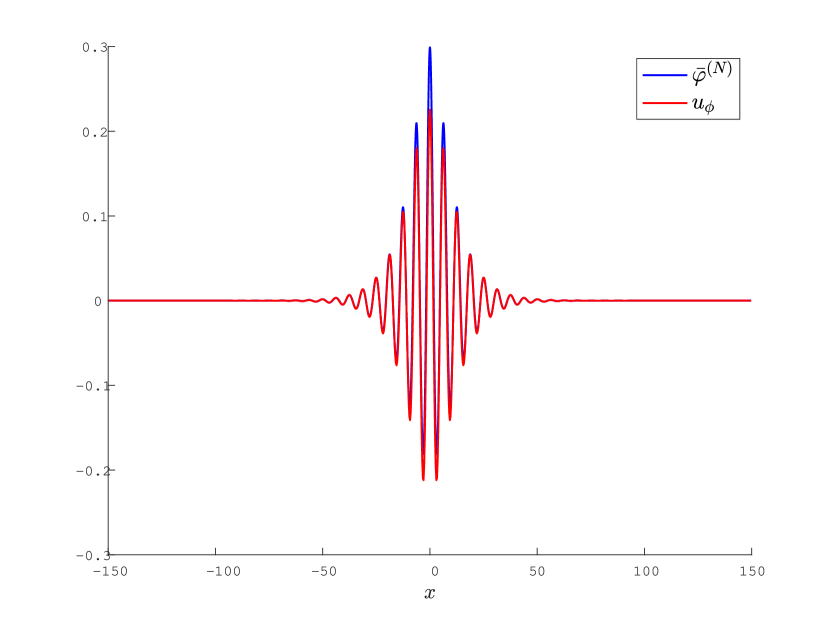
(a) $\phi=0$, $\nu=1.6$ and $\mu=0.05$

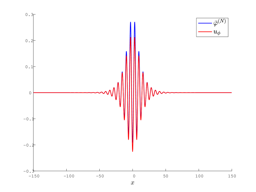
(b) $\phi=\pi$, $\nu=1.6$ and $\mu=0.05$

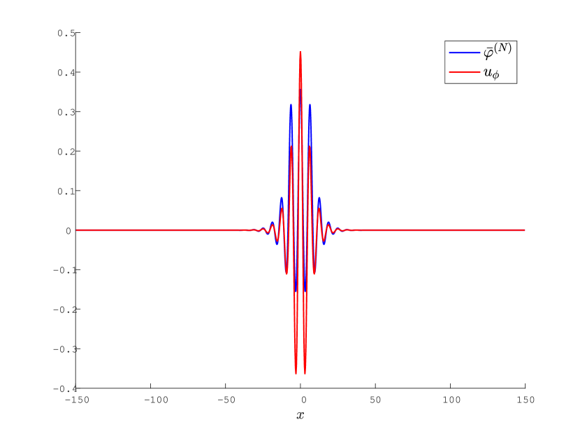
(c) $\phi=0$, $\nu=1.6$ and $\mu=0.2$.

Figure 10: Approximate symmetric pulse profiles using the normal form equation in (4.1) and after using Newton’s method on the Fourier coefficients.

Denote the vector of approximate Fourier coefficients obtained via Newton’s method for a pulse solution as $\bar{a}$. One can estimate the spectrum of the associated pulse solution by computing the eigenvalues of the matrix $DF(\bar{a})$. The eigenvalues for our example pulse solutions are given in Table 2. For the parameters $\nu=1.6$ and $\mu=0.05$, these results are consistent with the results found in [BK06].

Symmetric Pulse	Unstable Eigenvalues
$\varphi_{\phi}(x;\nu,\mu)$
$\varphi_{0}(x;1.6,0.05)$	0.1209
$\varphi_{\pi}(x;1.6,0.05)$	0.0058
	0.1179
$\varphi_{0}(x;1.6,0.2)$	N/A

Table 2: Approximate unstable eigenvalues for the three symmetric pulse solutions via Fourier methods.

4.2 Eigenvalues via Conjugate Points

We now compute the number of conjugate points for the two symmetric pulse solutions. We have shown there exists $L_{+}>0$ such that the conjugate points are all contained in the interval $(-\infty,L_{+}]$. In this work, our numerics serve as a proof-of-concept, so it is sufficient to choose $L_{cp}$ large via experimentation and compute the conjugate points on the interval from $[-L_{cp},L_{cp}]$.

In order to compute numerical approximations for the conjugate points associated to each pulse solution, we must first approximate the unstable subspace, $\mathbb{E}^{u,\phi}_{-}(x;0)$ on the interval from $[-L,L]$. The basis vectors for $\mathbb{E}^{u,\phi}_{-}(x;0)$ solve the nonautonomous system given by (1.8). We treat this as an autonomous problem by simultaneously computing the pulse $\varphi$ so that we can use ode45 in Matlab to integrate. After computing an approximation for the unstable subspace, we can use the following result to detect conjugate points.

Lemma 4.1.

Denote the frame matrix of $\mathbb{E}^{u}_{-}(x;0)$ as

$$\begin{pmatrix}M_{1}(x)\\ M_{2}(x)\\ M_{3}(x)\end{pmatrix},\qquad M_{1}(x),M_{3}(x)\in\mathbb{R}^{1\times 2},M_{2}(x)\in\mathbb{R}^{2\times 2}$$

and recall the reference plane $\ell_{*}^{sand}$ given in Definition 3.4. Then $\mathbb{E}^{u}_{-}(x;0)\cap\ell_{*}^{sand}\neq\{0\}$ if and only if $\det\begin{pmatrix}M_{1}(x)\\ M_{3}(x)\end{pmatrix}=0$.

Proof.

First, suppose that $\mathbb{E}^{u}_{-}(x)\cap\ell_{*}^{sand}\neq\{0\}$. Then by definition, there is a nonzero vector $v=(v_{1},v_{2})$ such that

$$\begin{pmatrix}M_{1}(x)\\ M_{2}(x)\\ M_{3}(x)\end{pmatrix}\begin{pmatrix}v_{1}\\ v_{2}\end{pmatrix}=\begin{pmatrix}0\\ \tilde{v}_{2}\\ \tilde{v}_{3}\\ 0\end{pmatrix},\qquad\qquad\tilde{v}_{2},\tilde{v}_{3}\in\mathbb{R}.$$

However, this means $\begin{pmatrix}M_{1}(x)\\ M_{3}(x)\end{pmatrix}v=0$. Thus, $\ker\begin{pmatrix}M_{1}(x)\\ M_{3}(x)\end{pmatrix}$ is nontrivial so $\det\begin{pmatrix}M_{1}(x)\\ M_{3}(x)\end{pmatrix}=0$.

Now suppose that $\det\begin{pmatrix}M_{1}(x)\\ M_{3}(x)\end{pmatrix}=0$. Then there is a vector $v$ such that $\begin{pmatrix}M_{1}(x)\\ M_{3}(x)\end{pmatrix}v=0$. Since $\mathbb{E}^{u}_{-}(x)$ is a Lagrangian subspace, its frame matrix has full rank, so

$$\begin{pmatrix}M_{1}(x)\\ M_{2}(x)\\ M_{3}(x)\end{pmatrix}\begin{pmatrix}v_{1}\\ v_{2}\end{pmatrix}=\begin{pmatrix}0\\ \tilde{v}_{2}\\ \tilde{v}_{3}\\ 0\end{pmatrix},$$

with at least one of $\tilde{v}_{2},\tilde{v}_{3}$ nonzero. Therefore, there is a nonzero vector in the intersection of $\mathbb{E}^{u}_{-}(x)$ and $\ell_{*}^{sand}$. ∎

Thus, we calculate the determinant of the submatrix formed from the first and fourth rows of the frame matrix for $\mathbb{E}^{u,\phi}_{-}(x;0)$, calculate the zeros corresponding to conjugate points. We fix $L_{cp}=60$ and compute

$$\mathbb{E}^{u,\phi}_{-}(x;0)=\begin{pmatrix}|&|\\ W^{-,u}_{1}&W^{-,u}_{2}\\ |&|\end{pmatrix}.$$

Define

$$\det A(x)=\det\begin{pmatrix}(W^{-,u}_{1})_{1}&(W^{-,u}_{2})_{1}\\ (W^{-,u}_{1})_{4}&(W^{-,u}_{2})_{4}\end{pmatrix}.$$

Via Lemma 4.1, the zeros of $\det A(x)$ correspond to conjugate points.

First, we look at the pulse solution with parameter values $\nu=1.6$, $\mu=0.05$ and phase condition $\phi=0$. This solution lies outside of the snaking region and we denote it via $\varphi_{0}(x;1.6,0.05)$. Via Fourier methods, we find one unstable eigenvalue (Figure 11(b)). When plotting the determinant of $A(x)$ associated to this pulse, we see that there is one zero (Figure 11(c)).

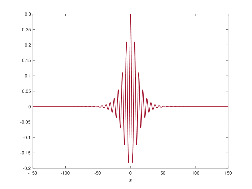
(a) Approximate pulse profile.

Unstable	Conjugate
Eigenvalues ($\lambda$)	Points ($x$)
0.1209	1.2400

(b) Unstable eigenvalues and conjugate points.

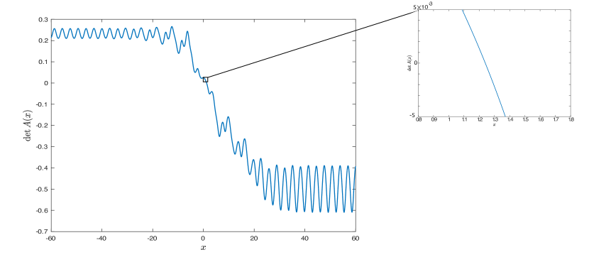
(c) $\det A(x)$ and the zero at $10^{-3}$ scale.

Figure 11: Information for the pulse with $\phi=0$, $\mu=0.05$ and $\nu=1.6$: $\varphi_{0}(x;1.6,0.05)$

Second, we look at the other symmetric pulse with parameter values $\nu=1.6$ and $\mu=0.05$ with phase condition $\phi=\pi$. We denote this pulse as $\varphi_{\pi}(x;1.6,0.05)$. Via Fourier spectral methods, we find two unstable eigenvalues (Figure 12(b)). By inspecting the plot of $\det A(x)$, we see that there are two zeros (Figure 12(c)).

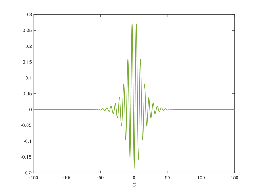
(a) Approximate pulse profile.

Unstable	Conjugate
Eigenvalues ($\lambda$)	Points ($x$)
0.0058	-0.6310
0.1179	17.5887

(b) Unstable eigenvalues and conjugate points.

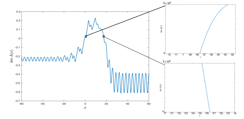
(c) $\det A(x)$ and the zeros at $10^{-3}$ scale.

Figure 12: Information for the pulse with $\phi=\pi$, $\mu=0.05$ and $\nu=1.6$: $\varphi_{\pi}(x;1.6,0.05)$

Taken together, the information about $\varphi_{\phi}(x;1.6,0.05)$, with $\phi=0,\pi$ contained in Figures 11 and 12 are consistent with results found in [BK06] and allow us to conclude that these two pulses are spectrally unstable. Since spectral stability in this case is necessary for linear and nonlinear stability, we see that these two pulses are linear/nonlinearly unstable as well.

Finally, we consider the symmetric pulse with parameter values $\nu=1.6$, $\mu=.20$ and phase condition $\phi=0$. This pulse lies within the parameter region that supports homoclinic snaking and is one of infinitely many asymmetric pulses for these parameter values. By performing Fourier spectral methods, we find no unstable eigenvalues. Additionally, when we plot $\det A(x)$, we see that there are no zeros. This information can be found in Figure 13.

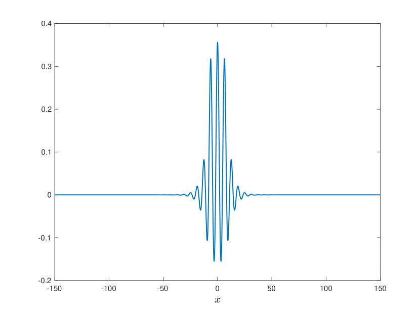
(a) Approximate pulse profile.

Unstable	Conjugate
Eigenvalues ($\lambda$)	Points ($x$)
N/A	N/A

(b) Unstable eigenvalues and conjugate points.

(c) $\det A(x)$.

Figure 13: Information for the pulse with $\phi=0$, $\mu=0.20$ and $\nu=1.6$: $\varphi_{0}(x;1.6,.20)$.

Remark 4.2.

The behavior at the tails of these plots are determined by the asymptotic coefficient matrix $B_{\infty}$ given in (1.13). Since $B_{\infty}$ has complex conjugate eigenvalues, we observe periodic behavior.

Another visualization of intersections between between the unstable subspace and the sandwich plane can be done via the Plücker coordinates. Given two vectors $v_{1}=\sum_{j=1}^{4}a_{j}e_{j}$ and $v_{2}=\sum_{j=1}^{4}b_{j}e_{j}$, the wedge product $v_{1}\wedge v_{2}$ is given by

$$v_{1}\wedge v_{2}=\sum_{i,j=1}^{4}(a_{i}b_{j}-a_{j}b_{i})(e_{i}\wedge e_{j}).$$

Definition 4.3.

Define the $ij$th Plücker coordinate as

$$P_{ij}=a_{i}b_{j}-a_{j}b_{i}.$$

Lemma 4.4 ([Lee03]).

The Lagrangian Grassmannian, $\Lambda(n)$ is a smooth manifold of dimension $\frac{1}{2}n(n+1)$.

Thus, $\Lambda(2)$ is $3$ dimensional, so we can use the chart given by $P_{12},P_{13}$ and $P_{14}$ to depict the sandwich plane and the trajectory of $\mathbb{E}^{u}_{-}(x)$ through $\Lambda(2)$ for the three pulse solutions we have considered thus far. One can compute that the train of $\ell_{*}^{sand}$ is given in these coordinates by

$$(P_{12},P_{13},P_{14})=(x,y,0),\qquad x,y\in\mathbb{R}.$$

For the parameters $\mu=0.05$ and $\nu=1.6$, we plot the pulse solution in standard coordinates and the trajectory of the unstable subspace in these Pluc̈ker coordinates. The train of $\ell_{*}^{sand}$ is depicted in purple. For the below two solutions, the trajectories intersect the sandwich plane a number of times that is consistent with the number of zeros in $\det A(x)$. This is not surprising, since these figures are a different visualization of the same analysis presented in Figures 11, 12 and 13.

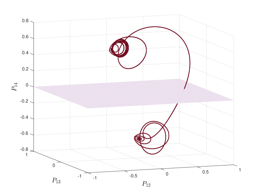
(a) $\varphi_{0}(x;1.6,0.05)$

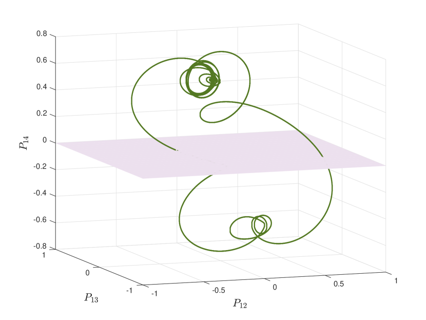
(b) $\varphi_{\pi}(x;1.6,0.05)$

Figure 15: Example symmetric pulse profiles (left) and the trajectory of the unstable subspace through $\Lambda(2)$ for each associated variational equation (right) for $\mu=0.05$ and $\nu=1.6$. The train of $\ell_{*}^{sand}$ is depicted in purple. Both of these pulse solutions are unstable.

Additionally, we plot the unstable subspace for the variational equation corresponding to the stable pulse with parameter values $\mu=0.20$ and $\nu=1.6$. In this case, we see that the entire trajectory of $\mathbb{E}^{u}_{-}(x)$ is bounded away from $\ell_{*}^{sand}$ in $\Lambda(2)$.

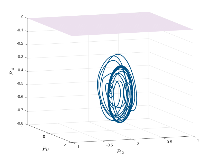
(a) $\varphi_{0}(x;1.6,0.20)$

Figure 17: Example symmetric pulse profile (left) and the trajectory of the unstable subspace through $\Lambda(2)$ for the variational equation (right) with $\mu=.20$ and $\nu=1.6$. The train of $\ell_{*}^{sand}$ is depicted in purple. This pulse solution is spectrally stable.

Remark 4.5.

The Matlab code for the results in this section is available online [BJP24].

5 Future Directions

In this work, we have shown that the number of unstable eigenvalues of pulse solutions to the Swift-Hohenberg equation corresponds to the number of conjugate points. Additionally, we have derived a novel numerical method for computing the stability of these solutions. However, the computations in Section 4 do not provide a mathematical proof of the spectral stability of pulse solutions. We are currently developing a method using validated numerics to do so, similar to that done in [BJ22]. In order to construct a computer assisted proof of the stability of a given solution $\varphi$, we must:

1. Compute a numerical approximation of $\varphi$ with error bounds;

2. determine the interval $[-L_{-},L_{+}]$ on which the conjugate points occur;

3. approximate $\mathbb{E}^{u}_{-}(-L_{-};0)$ and integrate forward to $\mathbb{E}^{u}_{-}(L_{+};0)$ with error bounds;

4. count the number of times $\mathbb{E}^{u}_{-}(x;0)$ intersects $\ell_{*}^{sand}$ for $x\in[-L_{-},L_{+}]$.

Computing $\mathbb{E}^{u}_{-}(x;0)$ on this interval is complicated by the presence of a so-called external resonance in the spatial eigenvalues. This resonance was also presence in the work of [BJ22], but the computer assisted proof in this work considered lower order approximations, so this was not an issue. We seek a higher order approximation of the subspace $\mathbb{E}^{u}_{-}(x;0)$ and so we must address this resonance.

Additionally, the use of higher order crossing forms could be used to prove a result relating the number of conjugate points to the number of unstable eigenvalues of the fourth order Hamiltonian system

$$u_{t}=-\partial_{x}^{4}u-P\partial_{x}^{2}u-u+u^{2}$$ (5.1)

where $P$ is a real parameter. In a certain parameter region, this system admits stationary localized solutions, which are studied in [Buf95, BCT96]. In [BCT96], these pulse solutions are classified via a sequence of integers $n(\ell_{1},\dots,\ell_{n-1})$, called the BCT classification, where $n$ is the number of major local extrema and $\ell_{i}$ are related to the number of zeros between the major local extrema. Numerical experiments suggest that the number of conjugate points associated to these solutions can be computed via the information encoded in the BCT classification [TJBD09]. If this were to be proved rigorously, this result could be viewed as an extension of Sturm-Liouville theory to fourth order systems. Rigorously justifying the results of [TJBD09] will be the subject of future work.

Appendix A Appendix

In the appendix, we provide the proofs of several technical lemmas and two explicit examples for which we compute the Maslov index with respect to a particular reference plane. One example has regular crossings and the other has nonregular crossings.

A.1 Proofs of technical results

A.1.1 Proof of Lemma 1.5

Here we present the proof of Lemma 1.5. This was relevant in the introduction when discussing the asymptotic behavior of the first order system we obtained by linearizing about the solution $\varphi$ given by (1.10).

Lemma 1.5. Let $B_{\infty}$ be as defined in (1.13). Then

1. $B_{\infty}(\lambda)$ is hyperbolic for all $\lambda\geq 0$.

2. The matrix $B_{\infty}$ depends analytically on $\lambda$. Also, there are positive constants $K_{B}$ and $C_{B}$, independent of $\lambda$, such that

   $$\|B(x;\lambda)-B_{\infty}(\lambda)\|\leq K_{B}e^{-C_{B}|x|}\text{ as }x\to\pm\infty.$$ (A.1)

Proof.

1. Using Hypothesis 1.2, a direct computation shows that the eigenvalues of $B_{\infty}(\lambda)$ are given via $\pm\gamma_{i}$, $i=1,2$ with $\gamma_{1}=\bar{\gamma}_{2}$ and $\text{Re}\gamma_{i}>0.$ We can express $\gamma_{1}$ as $\gamma_{1}=\sqrt{r}e^{i\theta/2}$, where

   $$\theta=\arctan\left(-\sqrt{\lambda-f^{\prime}(0)}\right)\quad\text{ and }r=\sqrt{1+\lambda-f^{\prime}(0)}.$$

   Since $f^{\prime}(0)<0$ and $\lambda\geq 0$, we have that $\theta\in(\frac{\pi}{2},\pi)$ and $r>1$.

2. Since $B_{\infty}$ is hyperbolic and $\lim_{x\to\pm}\varphi(x)=0$, it is a standard result that $B(x;\lambda)$ converges to its asymptotic limits at an exponential rate [KP13].

∎

A.1.2 Proof of Lemma 3.8

Here we present the proof of Lemma 3.8. This was a technical result that was used in Proposition 3.9, in which we proved that there are no intersections of $\mathbb{E}^{u}_{-}(-\infty,\lambda)$ and $\ell_{*}^{sand}$.

Lemma 3.8. Let $B_{\infty}$ be as defined in (1.13). If

$$\theta=\arctan\left(-\sqrt{\lambda-f^{\prime}(0)}\right)\quad\text{ and }r=\sqrt{1+\lambda-f^{\prime}(0)},$$

then basis vectors for the real unstable and stable eigenspaces of $B_{\infty}(\lambda)$ are given via

$$R^{u}_{1}=\begin{pmatrix}\frac{1}{r}\cos\theta\\ 1\\ \left(\frac{2}{\sqrt{r}}+\sqrt{r}\right)\cos\left(\frac{\theta}{2}\right)\\ \frac{1}{\sqrt{r}}\cos\left(\frac{\theta}{2}\right)\end{pmatrix},\quad R^{u}_{2}=\begin{pmatrix}-\frac{1}{r}\sin\theta\\ 0\\ \left(\sqrt{r}-\frac{2}{\sqrt{r}}\right)\sin\left(\frac{\theta}{2}\right)\\ -\frac{1}{\sqrt{r}}\sin\left(\frac{\theta}{2}\right)\end{pmatrix},$$ (A.2)

$$R_{1}^{s}=\begin{pmatrix}\frac{1}{r}\cos\theta\\ 1\\ \left(-\frac{2}{\sqrt{r}}-\sqrt{r}\right)\cos\left(\frac{\theta}{2}\right)\\ -\frac{1}{\sqrt{r}}\cos\left(\frac{\theta}{2}\right)\end{pmatrix},\quad R_{2}^{s}=\begin{pmatrix}-\frac{1}{r}\sin\theta\\ 0\\ \left(\frac{2}{\sqrt{r}}-\sqrt{r}\right)\sin\left(\frac{\theta}{2}\right)\\ \frac{1}{\sqrt{r}}\sin\left(\frac{\theta}{2}\right)\end{pmatrix}.$$ (A.3)

Proof.

Define $B_{\infty}(\lambda)$ by the block structure

$$B_{\infty}(\lambda)=\begin{pmatrix}0&0&0&1\\ 0&0&1&-2\\ -\lambda-1+f^{\prime}(0)&0&0&0\\ 0&1&0&0\end{pmatrix}:=\begin{pmatrix}0&P\\ Q&0\end{pmatrix}.$$

We will write the eigenvalues and eigenvectors of $B_{\infty}(\lambda)$ using information about the eigenvalues and eigenvectors of the matrix $PQ$. Via the properties of block matrices, we know that

$$\det\left(B_{\infty}(\lambda)-\gamma I_{4}\right)=\det\left(\gamma^{2}I_{2}-PQ\right).$$

Denote the eigenvalues of $PQ=\begin{pmatrix}0&1\\ -\lambda-1+f^{\prime}(0)&-2\end{pmatrix}$ by $\alpha_{k}$ with associated eigenvectors $v_{k}$, $k=1,2$. We can write these explicitly as

$$\begin{matrix}\alpha_{1}=-1+\sqrt{f^{\prime}(0)-\lambda}=-1+i\sqrt{\lambda-f^{\prime}(0)}:=re^{i\theta},&&v_{1}=\begin{pmatrix}1/\alpha_{1}\\ 1\end{pmatrix}=\begin{pmatrix}\frac{1}{r}e^{-i\theta}\\ 1\end{pmatrix}\\ \alpha_{2}=-1-\sqrt{f^{\prime}(0)-\lambda}=-1-i\sqrt{\lambda-f^{\prime}(0)}:=re^{-i\theta},&&v_{2}=\begin{pmatrix}1/\alpha_{2}\\ 1\end{pmatrix}:=\begin{pmatrix}\frac{1}{r}e^{i\theta}\\ 1\end{pmatrix}.\end{matrix}$$

(a) Eigenvalues of $PQ$

(b) Eigenvalues of $B_{\infty}(\lambda)$

Figure 18: Eigenvalues of $B_{\infty}(\lambda)$ understood through its block structure.

Then the eigenvalues of $B_{\infty}(\lambda)$ are given by $\pm\gamma_{k}=\pm\sqrt{\alpha_{k}}$, $k=1,2$. Relabeling as in Figure 18, define the vectors

$$V_{k}^{s}=\begin{pmatrix}v_{k}\\ -\gamma_{k}P^{-1}v_{k}\end{pmatrix}\text{ and }V_{k}^{u}=\begin{pmatrix}v_{k}\\ \gamma_{k}P^{-1}v_{k}\end{pmatrix}.$$ (A.4)

A direct computation shows that $(V^{s}_{k},-\gamma_{k})$ and $(V^{u}_{k},\gamma_{k})$ are eigenpairs for $B_{\infty}(\lambda)$ for $k=1,2$.

Finally, we can use the above characterizations of $\gamma_{k}$ and $v_{k}$ to write the eigenvectors of $B_{\infty}(\lambda)$. Taking real and imaginary parts yields the desired result.

∎

A.1.3 Representing Lagrangian Planes as Graphs: The technical details

Here we characterize the structure of the matrix whose graph is a given Lagrangian plane as is discussed at the beginning of Section 2, which was used in the proof of Theorem 2.14.

Let $\ell(t)$ be a Lagrangian path defined for $t\in[a,b]$ with frame matrix $L(t)$. Fix $t_{0}\in\mathbb{R}$ and let $\mathcal{W}$ be a Lagrangian plane such that $\ell(t_{0})\cap\mathcal{W}=\{0\}$. Then, there exists an $\epsilon>0$ and a $2n\times 2n$ matrix $A(t):\ell(t_{0})\to\mathcal{W}$ such that for all $v\in\ell(t_{0})$, $v\in\ker A(t_{0})$ and

$$v+A(t)v\in\ell(t),\qquad\ t\in(t_{0}-\epsilon,t_{0}+\epsilon).$$ (A.5)

Figure 19: Representing $\ell(t)$ as a graph for $t$ near $t_{0}$.

More generally, we have the following result:

Lemma A.1 ([lee]).

Let $\mathcal{V},\mathcal{W},\mathcal{P}\in\Lambda(n)$ such that $\mathcal{P}\cap\mathcal{W}=\{0\}$ and $\mathcal{V}\oplus\mathcal{W}=\mathbb{R}^{2n}$. Then, $\mathcal{P}$ can be written as the graph of a unique linear map $A:\mathcal{V}\to\mathcal{W}$.

We characterize the structure of the matrix $A$ in the following proposition.

Proposition A.2.

Suppose we are in the setting of Lemma A.1. Furthermore, let $B,C,D$ be symmetric $n\times n$ matrices. Then, the matrix $A:\mathcal{V}\to\mathcal{W}$ has the structure

$$A=\begin{pmatrix}B&C\\ D&-B^{T}\end{pmatrix}.$$ (A.6)

Proof.

For $v_{1},v_{2}\in\mathcal{V}$, we have that $v_{1}+Av_{1}$ and $v_{2}+Av_{2}$ are both in $\mathcal{W}$. Therefore,

$$0 =\omega(v_{1}+Av_{1},v_{2}+Av_{2})$$

$$=\omega(v_{1},v_{2})+\omega(v_{1},Av_{2})+\omega(Av_{1},v_{2})+\omega(Av_{1},Av_{2})$$

$$=\omega(v_{1},Av_{2})+\omega(Av_{1},v_{2})$$

$$=\langle v_{1},JAv_{2}\rangle+\langle v_{1},A^{T}Jv_{2}\rangle$$

$$=v_{1}^{T}\big{(}JA+A^{T}J\big{)}v_{2}.$$

If $\Pi_{\mathcal{V}}$ denotes the projection operator onto $\mathcal{V}$, then for all $x,y\in\mathbb{R}^{2n}$, we have

$$x^{T}\Pi_{\mathcal{V}}^{T}\big{(}JA+A^{T}J\big{)}\Pi_{\mathcal{V}}x=0.$$

Therefore, the Lagrangian property tells us that $\Pi^{T}_{\mathcal{V}}JA\Pi_{\mathcal{V}}=-\Pi^{T}A^{T}J\Pi_{\mathcal{V}}$. On the other hand, we can compute

$$\big{(}\Pi^{T}_{\mathcal{V}}JA\Pi_{\mathcal{V}}\big{)}^{T}=\Pi^{T}_{\mathcal{V}}A^{T}J^{T}\Pi_{\mathcal{V}}=-\Pi^{T}_{\mathcal{V}}A^{T}J\Pi_{\mathcal{V}}.$$

By putting these pieces together, we see that

$$\big{(}\Pi_{\mathcal{V}}^{T}JA\Pi_{\mathcal{V}}\big{)}^{T}=\Pi^{T}_{\mathcal{V}}JA\Pi_{\mathcal{V}}\big{)},$$ (A.7)

so this matrix is symmetric. Since $\Pi_{\mathcal{V}}^{T}=\Pi_{\mathcal{V}}$, we can derive the necessary structure of $A$ such that $(JA)^{T}=JA$ to obtain a matrix that satisfies (A.7). If we represent $A$ with the block structure $B,C,D,E$, we see that

$$JA =\begin{pmatrix}0&-I_{n}\\ I_{n}&0\end{pmatrix}\begin{pmatrix}B&C\\ D&E\end{pmatrix}=\begin{pmatrix}-D&-E\\ B&C\end{pmatrix}$$

$$(JA)^{T} =\begin{pmatrix}-D^{T}&B^{T}\\ -E^{T}&C^{T}\end{pmatrix}.$$

Thus $JA=(JA)^{T}$ if $D$ and $C$ are symmetric and $-E=B^{T}$. Finally, we see that since the matrix $\Pi_{\mathcal{V}}A(t)$ is unique and we have derived such a matrix satisfying the necessary conditions, we can assume $A$ has the structure given in (A.6). ∎

A.2 An Explicit Example with the Maslov Index

Here we present an explicit example using a path of Lagrangian subspaces whose basis vectors are constructed from solutions to an ODE. We compute the Maslov index with respect to the sandwich plane using the crossing form. This example serves two purposes. The first is to illustrate the subtlety in expressing a path of Lagrangian subspaces as a graph that is discussed in Remark 3.12. The second is to concretely show the relationship between the higher order crossing forms and the derivatives of the eigenvalues of the graph matrix (see Section 2.3).

Consider the autonomous differential equation

$$\dot{q}=\underbrace{\begin{pmatrix}0&0&1&0\\ 0&0&0&0\\ 0&-1&0&0\\ -1&0&0&0\end{pmatrix}}_{:=B}q=\underbrace{\begin{pmatrix}0&0&1&0\\ 0&0&0&1\\ -1&0&0&0\\ 0&-1&0&0\end{pmatrix}}_{:=J}\underbrace{\begin{pmatrix}0&1&0&0\\ 1&0&0&0\\ 0&0&1&0\\ 0&0&0&0\end{pmatrix}}_{:=C}q.$$ (A.8)

This system has a general solution given by

$$\begin{split}q_{1}(s)&=-\frac{C_{2}}{2}s^{2}+C_{3}s+C_{1}\\ q_{2}(s)&=C_{2}\\ q_{3}(s)&=-C_{2}s+C_{3}\\ q_{4}(s)&=\frac{C_{2}}{6}s^{3}-\frac{C_{3}}{2}s^{2}-C_{1}s+C_{4}.\end{split}$$ (A.9)

A.2.1 Regular Crossings

Consider the Lagrangian plane

$$\ell_{1}(s)=\text{colspan}\begin{pmatrix}|&|\\ v_{1}(s)&v_{2}(s)\\ |&|\end{pmatrix}:=\text{colspan}\begin{pmatrix}-\frac{1}{2}s^{2}+2s&-3s^{2}+1\\ 1&6\\ 2-s&-6s\\ \frac{1}{6}s^{3}-s^{2}&s^{3}-s+2\end{pmatrix}.$$

Note that this pair of solutions to the above ODE satisfies the Lagrangian condition. The first spanning vector intersects $\ell_{*}^{sand}$ at $s=0$. We will use the crossing form to understand how this crossing contributes to the Maslov index. To do so, we first want to write $\ell_{1}(s)$ as a graph. Suppose that $A_{1}(s):\ell_{1}(0)\to(\ell_{*}^{sand})^{\perp}$ where

$$\big{(}\ell_{*}^{sand}\big{)}^{\perp}=\text{colspan}\begin{pmatrix}1&0\\ 0&0\\ 0&0\\ 0&1\end{pmatrix}.$$

Remark A.3.

It is clear from this example that there is no such matrix $A_{1}(s):\ell_{1}(0)\to(\ell_{*})^{\perp}$ that leaves $v_{1}(0)$ invariant, meaning $v_{1}(0)+A_{1}(s)v_{1}(0)=v_{1}(s)$. The problem arises in the third component. To see this explicitly, we can write

$$\begin{pmatrix}0\\ 1\\ 2\\ 0\end{pmatrix}+A_{1}(s)\begin{pmatrix}0\\ 1\\ 2\\ 0\end{pmatrix}=\begin{pmatrix}f_{1}(s)\\ 1\\ 2\\ f_{2}(s)\end{pmatrix}\neq\begin{pmatrix}-\frac{1}{2}s^{2}+2s\\ 1\\ 2-s\\ \frac{1}{6}s^{3}-s^{2}\end{pmatrix}.$$

There are no such $f_{1}(s),f_{2}(s)$ that could satisfy this relationship.

We seek a matrix $A_{1}(s):\ell_{1}(0)\to\mathcal{(}\ell_{*})^{\perp}$ having the structure given in Proposition A.2 such that for $k_{1},k_{2}\in\mathbb{R}$,

$$k_{1}\begin{pmatrix}0\\ 1\\ 2\\ 0\end{pmatrix}+k_{2}\begin{pmatrix}1\\ 6\\ 0\\ 2\end{pmatrix}+A_{1}(s)\begin{pmatrix}k_{2}\\ k_{1}+6k_{2}\\ 2k_{1}\\ 2k_{2}\end{pmatrix}=c_{1}\begin{pmatrix}-\frac{1}{2}s^{2}+2s\\ 1\\ 2-s\\ \frac{s^{3}}{6}-s^{2}\end{pmatrix}+c_{2}\begin{pmatrix}-3s^{2}+1\\ 6\\ -6s\\ s^{3}-s+2\end{pmatrix}.$$ (A.10)

By focusing our attention on the middle two components of $A_{1}(s)\big{(}k_{1}v_{1}(0)+k_{2}v_{2}(0)\big{)}$, which are $0$ by assumption, we derive

$$c_{1} =\left(\frac{s}{2}+1\right)k_{1}+(3s)k_{2}$$

$$c_{2} =\left(-\frac{1}{12}s\right)k_{1}+\left(1-\frac{1}{2}s\right)k_{2}.$$

There is one degree of freedom in this system and we find that a solution is given by

$$A_{1}(s)=\begin{pmatrix}3s^{2}-\frac{1}{2}&0&\frac{1}{4}s^{2}+\frac{23}{24}s&0\\ a_{21}&0&0&-\frac{1}{2}a_{21}\\ -36s^{2}+6s+2a_{21}&6s^{2}-s&-\frac{1}{2}(6s^{2}-s)&-a_{21}\\ 6s^{2}-s&\frac{1}{12}(4s^{3}-11s^{2}-2s)&0&0\end{pmatrix}.$$ (A.11)

Let $\Pi_{1}$ be the projection onto $\ell_{1}(0)\cap\ell_{*}=v_{1}(0)$. This matrix can be calculated explicitly as

$$\Pi_{1}=v_{1}(0)\left(v_{1}(0)^{T}v_{1}(0)\right)^{-1}v_{1}(0)^{T}=\frac{1}{5}\begin{pmatrix}0&0&0&0\\ 0&1&2&0\\ 0&2&4&0\\ 0&0&0&0\end{pmatrix}.$$

Using $\Pi_{1}$ given above, we can explicitly compute the matrix that determines the crossing form as

$$\Pi_{1}JA_{1}(s)\Pi_{1}=-\frac{s}{150}\left(4s^{2}+23s+48\right)\begin{pmatrix}0&0&0&0\\ 0&\frac{1}{2}&1&0\\ 0&1&\frac{1}{2}&0\\ 0&0&0&0\end{pmatrix}.$$

The eigenvalues of $\Pi_{1}JA_{1}(s)\Pi_{1}$ determine whether this crossing contributes positively or negatively to the Maslov index. The first order crossing form (Defintion 2.1) captures the sign of the first derivative of this eigenvalue. We can calculate that $\Pi_{1}JA_{1}(s)\Pi_{1}$ has three uniformly $0$ eigenvalues and one $s$-dependent eigenvalue given by

$$\lambda(s)=-\frac{1}{15}s^{3}-\frac{23}{60}s^{2}-\frac{4}{5}s.$$ (A.12)

The crossing form calculates the sign of this derivative. We can calculate that

$$Q^{(1)}(v_{1}(0))=\langle v_{1}(0),JA_{1}^{\prime}(0)v_{1}(0)\rangle=-4.$$

On the other hand, we can differentiate directly to see that

$$\lambda^{\prime}(0)=-\frac{4}{5}.$$

Note that $\lambda^{\prime}(0)$ and $Q^{(1)}(v_{1}(0))$ are off by a factor of $5$. If we want to directly apply Theorem 2.25 to conclude $\lambda^{\prime}(0)=Q^{(1)}(v_{1}(0))$, we first need to normalize $v_{1}(0)$.

We can also use (A.10) to calculate the crossing form without explicitly knowing the structure of $A_{1}(s)$. With $k_{1}=1$ and $k_{2}=0$, we have that

$$c_{1}(s) =\left(\frac{s}{2}+1\right)$$

$$c_{2}(s) =-\frac{1}{12}(s).$$

Using this, we can calculate

$$Q^{(1)}(v_{1}(0)) =\big{\langle}v_{1}(0),JA_{1}^{\prime}(0)v_{1}(0)\big{\rangle}$$

$$=\left\langle v_{1}(0),J\big{(}c_{1}^{\prime}(0)v_{1}(0)+c_{1}(0)v_{1}^{\prime}(0)+c_{2}^{\prime}(0)v_{2}(0)+c_{2}(0)v_{2}^{\prime}(0)\big{)}v_{1}(0)\right\rangle$$

$$=\langle v_{1}(0),Jv^{\prime}_{1}(0)\rangle$$

$$=\langle v_{1}(0),JBv_{1}(0)\rangle$$

$$=-4.$$

A.2.2 Non-regular Crossings

We now consider a path of Lagrangian planes with a nonregular crossing. Consider the Lagrangian plane

$$\ell_{2}(s)=\text{colspan}\begin{pmatrix}|&|\\ v_{1}(0)&v_{2}(0)\\ |&|\end{pmatrix}:=\text{colspan}\begin{pmatrix}-\frac{s^{2}}{2}&-3s^{2}+1\\ 1&6\\ -s&-6s\\ \frac{s^{3}}{6}&s^{3}-s\end{pmatrix}$$

satisfying (A.8). The first spanning vector intersects $\ell_{*}^{sand}$ at $s=0$.

As in the previous example, we want to calculate the contribution of this intersection to the Maslov index with respect to the sandwich plane by using the crossing form. For $s$ sufficiently small, we can write $\ell_{2}(s)$ as the graph of a matrix $A_{2}(s)\in\mathbb{R}^{4\times 4}$ having the structure given in Proposition A.2. Furthermore, we want $A_{2}(s):\ell_{2}(0)\to\ell_{2}(0)^{\perp}$. Note that we do not seek $A_{2}(s):\ell_{2}(0)\to(\ell_{*})^{\perp}$ because $(\ell_{*})^{\perp}\cap\ell_{2}(0)\neq\{0\}$. With these assumptions $A_{2}(s)$ must satisfy the equation

$$\begin{split}k_{1}\begin{pmatrix}0\\ 1\\ 0\\ 0\end{pmatrix}+k_{2}\begin{pmatrix}1\\ 6\\ 0\\ 0\end{pmatrix}+A_{2}(s)&\begin{pmatrix}k_{2}\\ k_{1}+6k_{2}\\ 0\\ 0\end{pmatrix}=c_{1}\begin{pmatrix}-\frac{s^{2}}{2}\\ 1\\ -s\\ \frac{s^{3}}{6}\end{pmatrix}+c_{2}\begin{pmatrix}-3s^{2}+1\\ 6\\ -6s\\ s^{3}-s\end{pmatrix}\\ \end{split}$$ (A.13)

we find that $c_{1}$ and $c_{2}$ satisfy

$$c_{1} =k_{1}-3s^{2}(k_{1}+6k_{2})$$

$$c_{2} =k_{2}+\frac{1}{2}s^{2}(k_{1}+6k_{2}).$$

By substituting these equations in for $c_{1}$ and $c_{2}$ and solving this system of equations, we find a matrix satisfying (A.13) to be

$$A_{2}(s)=\begin{pmatrix}0&0&a_{13}&a_{14}\\ 0&0&a_{14}&a_{24}\\ 0&-s&0&0\\ -s&-\frac{s^{3}}{3}&0&0\end{pmatrix}.$$

Note that $a_{13},a_{14}$ and $a_{24}$ are free.

Define $\Pi_{2}$ to be the projection matrix onto $\ell_{*}\cap\ell_{2}(0)$. We can compute that

$$\Pi_{2}=\begin{pmatrix}0&0&0&0\\ 0&1&0&0\\ 0&0&0&0\\ 0&0&0&0\end{pmatrix}.$$

Then, the sign of the crossing form tracks how the sign of the nonzero eigenvalue of $\Pi_{2}JA_{2}(s)\Pi_{2}$ changes as $s$ increases through $0$. Because $A_{2}(s)$ is explicitly known, we can calcualate this as

$$\Pi_{2}JA(s)\Pi_{2}=\begin{pmatrix}0&0&0&0\\ 0&-\frac{1}{3}s^{3}&0&0\\ 0&0&0&0\\ 0&0&0&0\end{pmatrix}.$$

This matrix has $3$ zero eigenvalues and one $s$-dependent eigenvalue given by

$$\lambda_{1}(s)=-\frac{1}{3}s^{3}.$$

Since this eigenvalue is decreasing through $0$, we expect the intersection of $\ell_{2}(s)$ and $\ell_{*}^{sand}$ at $s=0$ to contribute negatively to the Maslov index.

The vector $v=\begin{pmatrix}0&1&0&0\end{pmatrix}$ is in $\ell_{*}\cap\ell_{2}(0)$. If we compute the first order crossing form, we find

$$Q^{(1)}(v) =\big{\langle}v,JA_{2}^{\prime}(0)v\big{\rangle}$$

$$=\begin{pmatrix}0&0&0&1\end{pmatrix}\begin{pmatrix}0\\ 1\\ -1\\ -s^{2}\end{pmatrix}\bigg{|}_{s=0}$$

$$=-s^{2}\bigg{|}_{s=0}$$

$$=0.$$

Proceeding similarly, we find that

$$Q^{(2)}(0) =\big{\langle}v_{1}(0),JA_{2}^{\prime\prime}(0)v_{1}(0)\big{\rangle}$$

$$=0$$

$$Q^{(3)}(0) =\big{\langle}v_{1}(0),JA_{2}^{(3)}(0)v_{1}(0)\big{\rangle}$$

$$=-2.$$

If we did not know $\lambda(s)$ explicitly, we could use Theorem 2.21 to conclude that this crossing contributes negatively to the Maslov index. Theorem 2.25 tells us that this means $\lambda(s)$ must be decreasing at $s=0$.

If we didn’t explicitly know $A_{2}(s)$ (as is the case with many applications to differential equations), we can use the general structure in (A.13) to calculate the sign of the third crossing form. If we set $k_{1}=1$ and $k_{2}=0$, then $c_{1}(s)=1-3s^{2}$ and $c_{2}(s)=\frac{1}{2}s^{2}$. In this case, we have

$$Q^{(3)}(v_{1}(0)) =\left\langle v_{1}(0),JA^{(3)}(0)v_{1}(0)\right\rangle$$

$$=\underbrace{\langle v_{1}(0),J\left(c_{1}^{\prime\prime\prime}(0)v_{1}(0)+c_{2}^{\prime\prime\prime}(0)v_{2}(0)\right)\rangle}_{=0\text{ via Lag. prop.}}+3\langle v_{1}(0),J\left(c_{1}^{\prime\prime}(0)v_{1}^{\prime}(0)+c_{2}^{\prime\prime}(0)v_{2}^{\prime}(0)\right)\rangle$$

$$\qquad+\underbrace{3\langle v_{1}(0),J(c_{1}^{\prime}(0)v_{1}^{\prime\prime}(0)+c_{2}^{\prime}(0)v_{2}^{\prime\prime}(0))\rangle}_{0\text{ since }c_{1}^{\prime}(0)=c_{2}^{\prime}(0)=0}+\langle v_{1}(0),J(c_{1}(0)v_{1}^{\prime\prime\prime}(0)+\underbrace{c_{2}(0)}_{=0}v_{2}^{\prime\prime\prime}(0))\rangle$$

$$=3c_{1}^{\prime\prime}(0)\underbrace{\langle v_{1}(0),Jv_{1}^{\prime}(0)\rangle}_{=Q^{(1)}(v_{1}(0))=0}+3c_{2}^{\prime\prime}(0)\langle v_{1}(0),Jv_{2}^{\prime}(0)\rangle+\langle v_{1}(0),J(c_{1}(0)v_{1}^{\prime\prime\prime}(0)\rangle$$

$$=3\langle v_{1}(0),JBv_{2}(0)\rangle+\langle v_{1}(0),JBBBv_{1}(0)\rangle$$

$$=-3+1$$

$$=-2.$$

References

• [ACLS08] Daniele Avitabile, Alan Champneys, David J. B. Lloyd, and Björn Sanstede. Localized hexagon patterns of the planar swift-hohenberg equation. SIAM Journal on Applied Dynamical Systems, 7:1049–1100, 2008.
• [Arn67] V.I. Arnol’d. Characteristic class entering in quantization conditions. Functional Analysis and its Applications, 1:1–13, 1967.
• [Arn85] V.I. Arnol’d. Sturm theorems and symplectic geometry. Functional Analysis and its Applications, 19:1–10, 1985.
• [BCJ+18] M. Beck, G. Cox, C. K. R. T. Jones, Y. Latushkin, K. McQuighan, and A. Sukhtayev. Instability of pulses in gradient reaction-diffusion systems: a symplectic approach. Philos. Trans. Roy. Soc. A, 376(2117):20170187, 20, 2018.
• [BCT96] B. Buffoni, A. R. Champneys, and J.F. Toland. Bifurcation and coalescence of a plethora of multi-modal homoclinic orbits in a Hamiltonian system. Journal of Dynamics and Differential Equations, 8:221–281, 1996.
• [BJ22] Margaret Beck and Jonathan Jaquette. Validated spectral stability via conjugate points. SIAM J. Applied Dynamical Systems, 21:366–404, 2022.
• [BJP24] M. Beck, J. Jaquette, and H. Pieper. Codes for “the Maslov index, degenerate crossings and the stability of pulse solutions to the Swift-Hohenberg equation”. https://github.com/hpieper14/Swift-Hohenberg-stability, 2024.
• [BK06] J. Burke and E. Knobloch. Localized states in the generalized Swift-Hohenberg equation. Phys. Rev. E, 73, 2006.
• [BK07a] J. Burke and E. Knobloch. Homoclinic snaking: Structure and stability. Chaos: An Interdisciplinary Journal of Nonlinear Science, 17, 2007.
• [BK07b] J. Burke and E. Knobloch. Normal form for spatial dynamics in the Swift-Hohenberg equation. Discrete and Continuous Dynamical Systems, 2007.
• [BK07c] J. Burke and E. Knobloch. Snakes and ladders: Localized states in the Swift-Hohenberg equation. Physics Letters A, 360:681–688, 2007.
• [BKL+09a] Margaret Beck, Jürgen Knobloch, David Lloyd, Björn Sandstede, and Thomas Wagenknecht. Snakes, ladders, and isolas of localized patterns. SIAM Journal on Mathematical Analysis, 41:936–972, 2009.
• [BKL+09b] Margaret Beck, Jürgen Knobloch, David J. B. Lloyd, Björn Sandstede, and Thomas Wagenknecht. Snakes, ladders and isolas of localized patterns. SIAM Journal on Mathematical Analysis, 41:936–972, 2009.
• [Bot56] R. Bott. On the iteration of closed geodesics and Sturm intersection theory. Comm. Pure Appl. Math., 2:171–206, 1956.
• [Buf95] B. Buffoni. Infinitely many large-amplitude homoclinic orbits for a class of autonomous Hamiltonian systems. Indiana University Math Journal, 121:109–120, 1995.
• [CCLM23] Graham Cox, Mitchell Curran, Yuri Latushkin, and Robert Marangell. Hamiltonian spectral flows, the maslov index, and the stability of standing waves in the nonlinear schrodinger equation. SIAM Journal on Mathematical Analysis, 55(5):4998–5050, 2023.
• [CH93] M. Cross and P. Hohenberg. Oscillon-type structures and their interaction in a swift-hohenberg model. Rev. Modern Phys., 65:851 – 1112, 1993.
• [CJLS16] G. Cox, C. K. R. T. Jones, Y. Latushkin, and A. Sukhtayev. The Morse and Maslov index for multidimensional Schrodinger operators with matrix-valued potentials. Trans. Amer. Math. Soc., 368:8145 – 8207, 2016.
• [CJM15] Graham Cox, Chris Jones, and Jeremy Marzoula. A Morse index theorem for elliptic operators on bounded domains. Comm. Partial Differential Equations, 40:1467–1497, 2015.
• [CJM17] Graham Cox, Chris Jones, and Jeremy Marzoula. Manifold decompositions and indices of Schrödinger operators. Indiana University Mathematics Journal, 66:1573–1602, 2017.
• [Cop78] W. A. Coppel. Dichotomies in Stability Theory, volume 629 of Lecture Notes in Mathematics. Springer, Berlin, Germany, 1978.
• [Dan08] Daniel Daners. Handbook of Differential Equations: Stationary Partial Differential Equations, volume 6. Elsevier, 2008.
• [DJ11] Jian Deng and Chris Jones. Multi-dimensional Morse index theorems and a symplectic view of ellptic boundary conditions. Transactions of the American Mathematical Society, 363:1487–1508, 2011.
• [Dui76] J.J. Duistermaat. On the Morse index in variational calculus. Advances in Mathematics, pages 173–195, 1976.
• [Edw64] H. M. Edwards. A generalized Sturm theorem. Ann. of Math, pages 22–57, 1964.
• [Fur04] Kenro Furutani. Fredholm-Lagrangian-Grassmannian and the Maslov index. Journal of Geometry and Physics, 51:269–331, 2004.
• [Hen81] Daniel Henry. Geometric Theory of Semilinear Parabolic Equations. Springer Berlin, Heidelberg, 1981.
• [HLS18] Peter Howard, Yuri Latishkin, and Alim Sukhtayev. The Maslov and Morse indices for Schrödinger operators on $\mathbb{r}$. Indiana Univ. Math Journal, 67:1765–1815, 2018.
• [How21a] Peter Howard. Hörmander’s index and oscillation theory”. Journal of Mathematical Analysis and Applications, 500:233–277, 2021.
• [How21b] Peter Howard. The maslov index and spectral counts for linear hamiltonian systems on $\mathbb{R}$. Journal of Dynamics and Differential Equations, 35, 09 2021.
• [HS77] P.C. Hohenberg and J. Swift. Hydrodynamic fluctuations at the convective instabilitiy. Phys. Rev. A, 15:319 – 328, 1977.
• [HS16] Peter Howard and Alim Sukhtayev. The Maslov and Morse indices for Schrödinger operators on [0,1]. Journal of Differential Equations, 260:4499–4549, 2016.
• [Jon88] Chris Jones. Instability of standing waves for nonlinear Schrödinger-type equations. Ergodic Theory Dynam. Systems, 8:119–138, 1988.
• [Kat66] Tosio Kato. Perturbation Theory for Linear Operators. Springer, New York, 1966.
• [KP13] Todd Kapitula and Keith Promislow. Spectral and Dynamical Stability of Nonlinear Waves. Springer, New York, 2013.
• [Lan64] P. Lancaster. On eigenvalues of matrices dependent on a parameter. Numerische Mathematik, 6:377–387, 1964.
• [Lee03] John M. Lee. Introduction to Smooth Manifolds. Springer, New York, 2003.
• [MS17] D. McDuff and D. Salamon. Introduction to Symplectic Topology. Oxford Academic, Oxford, UK, 3rd edition, 2017.
• [MS19] Elizabeth Makrides and Björn Sandstede. Existence and stability of spatially localized patterns. Journal of Differential Equations, 266:1073–1120, 2019.
• [RGP04] Paolo Piccione Roberto Giambo and Alessandro Portaluri. Computation of the maslov index and the spectral flow via partial signaturees. C. R. Math. Acad. Sci, pages 397–402, 2004.
• [RS93] J. Robbin and D. Salamon. The Maslov index for paths. Topolgy, 32:827–844, 1993.
• [Sma65] S. Smale. On the Morse index theorem. J. Math. Mech, pages 1049–1055, 1965.
• [SS00] Björn Sandstede and Arnd Scheel. Absolute and convective instabilities of waves on unbounded and large bounded domains. Physica D: Nonlinear Phenomena, 143:233–277, 2000.
• [TJBD09] F. Chardard T. J. Bridges and F. Dias. On the Maslov index of multi-pulse homoclinic orbits. Proceedings of the Royal Society A: Mathematical, Physical and Engineering Sciences, 465:2897–2910, 2009.