Personalized Negative Reservoir for Incremental Learning in Recommender Systems

Abstract.

Recommender systems have become an integral part of online platforms. Every day the volume of training data is expanding and the number of user interactions is constantly increasing. The exploration of larger and more expressive models has become a necessary pursuit to improve user experience. However, this progression carries with it an increased computational burden. In commercial settings, once a recommendation system model has been trained and deployed it typically needs to be updated frequently as new client data arrive. Cumulatively, the mounting volume of data is guaranteed to eventually make full batch retraining of the model from scratch computationally infeasible. Naively fine-tuning solely on the new data runs into the well-documented problem of catastrophic forgetting. Despite the fact that negative sampling is a crucial part of training with implicit feedback, no specialized technique exists that is tailored to the incremental learning framework. In this work, we take the first step to propose, a personalized negative reservoir strategy which is used to obtain negative samples for the standard triplet loss. This technique balances alleviation of forgetting with plasticity by encouraging the model to remember stable user preferences and selectively forget when user interests change. We derive the mathematical formulation of a negative sampler to populate and update the reservoir. We integrate our design in three SOTA and commonly used incremental recommendation models. We show that these concrete realizations of our negative reservoir framework achieve state-of-the-art results in standard benchmarks, on multiple standard top-k evaluation metrics.

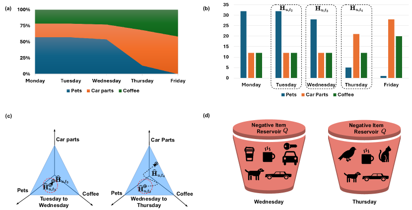
Figure 1. Toy example with daily model updates with 3 item categories: pet items, car part items and coffee items. The figure shows a user’s interactions with these categories over a week. (a) User $u$ interacts with more items from pet item category in the start of the start of the week but his interests change over time and he interacts with more car part items by the end of the week. (b) The change of preference is reflected on the histograms of user-item categories $\mathbf{H}_{u,t}$. (c) The histograms are normalized $\widehat{\mathbf{H}}_{u,t}$ and projected on the simplex $\Delta_{2}$. There we see the interest shift on the simplex representing the user’s interest shift from $t=2,$ (Tuesday) to $t=3$, (Wednesday) and on the right the user’s interest shift from $t=3,$ (Wednesday) to $t=4$, (Thursday). We see that the user exhibits a large change in interests on the right (moves far away from current neighborhood in simplex denoted by a red dashed circle). (d) We propose to sample more negatives from pet category when fine tuning the model on Thursday to allow the model to quickly adjust to new user interests (in the figure the right bucket has many more pet related items).

1. Introduction

Recommender systems have become a crucial part of online services. Delivering highly relevant item recommendations not only enhances user experience but also bolsters the revenue of service providers. The advent of deep learning-based recommender systems (Covington et al., 2016; Guo et al., 2017; Cheng et al., 2016; He et al., 2023) has significantly elevated the quality of user and item representations. To more accurately represent user behavior, there has been a substantial expansion in the volume of training data, accumulated from the long user-item interaction history (He et al., 2023; Xu et al., 2020). Thus, the exploration of larger and more expressive models has become a vital research direction. For example, Graph Neural Network (GNN) (Kipf and Welling, 2017) based recommendation methods can achieve compelling performance on recommendation tasks because of their ability to model the rich relational information of the data through the message passing paradigm (van den Berg et al., 2018; Wang et al., 2019a, 2021a; Sun et al., 2019). However, this evolution brings with it a potential increase in computational burden. An industrial-scale recommendation serving model, once integrated into an online system, usually requires regular updates to accommodate the arrival of recent client data. The constant arrival of new data inevitably leads to a point where full-batch retraining of the model from scratch becomes infeasible.

One straightforward way to tackle this computational challenge is to train the backbone model in an incremental fashion, updating it only when a new data block arrives, instead of full batch retraining with older data. In industrial-level recommender systems, the new data block can arrive in a daily, hourly or even a shorter interval (Xu et al., 2020; Wang et al., 2021b), depending on the application. Unfortunately, naively fine-tuning the model with new data leads to the well-known issue of “catastrophic forgetting” (Kirkpatrick et al., 2017), i.e., the model discards information from earlier data blocks and overfits to the newly acquired data. There are two mainstream methods to alleviate the catastrophic forgetting problem: (i) experience (reservoir) replay (Prabhu et al., 2020; Ahrabian et al., 2021), and (ii) regularization-based knowledge distillation (Castro et al., 2018; Kirkpatrick et al., 2017; Xu et al., 2020; Wang et al., 2021b, 2023). Reservoir replay methods retrain on some previously observed user interactions from past data blocks while jointly training with the new data. The regularization techniques are typically formulated as a knowledge distillation problem where the model trained on the old data takes the role of the “teacher” model and the model fine-tuned on the new data is regarded as the “student” model. A knowledge distillation loss is applied to preserve the information from the teacher to the student model through model weight distillation (Castro et al., 2018; Kirkpatrick et al., 2017), structural (Xu et al., 2020), or contrastive distillation (Wang et al., 2021b).

However, there is one important aspect of the incremental learning framework that has received very little attention. Negative sampling plays a critical role in recommendation system training. The most common strategy for negative sampling involves uniform random sampling of the negatives (Rendle et al., 2009). While subsequent works improve upon the negative sampler for the static setting (one-time learning), there are no works dedicated to addressing negative sampling in the incremental learning setting. We identify two unique challenges for designing a good negative sampler for an incremental learning framework. First, the negative reservoir must be personalized for each user, and notably, it should model a user’s interests or preference shift across consecutive time blocks. This can provide a significant distribution bias in the negative sampling process. This relates to a classic trade-off in online learning, achieving a correct balance in retaining knowledge learned from prior training (stability), and being flexible enough to learn concepts from new observations (plasticity). Second, the ranking list (prediction) produced by the model from the previous time block should be exploited in order to find informative negative samples for the training in the new block.

Considering the above-mentioned challenges, we design the first negative reservoir strategy tailored for the incremental learning framework. This negative reservoir contains the most effective negative samples in each incremental training block based on the user change of interest. Our negative reservoir design is compatible with almost all existing incremental learning frameworks for recommender systems. In our experiments, we integrate our negative reservoir design into three recent incremental learning frameworks. Our designed negative reservoir achieves state-of-the-art performance when incorporated in three standard incremental learning frameworks, improving GraphSAIL (Xu et al., 2020), SGCT (Wang et al., 2021b), and LWC-KD (Wang et al., 2021b) by an average of 13.4%, 9.4% and 6.7%, respectively, across five large-scale recommender system datasets. Our main contributions can be summarized as:

• This is the first work to propose a negative reservoir design tailored for incremental learning in recommender systems. The approach, for which we provide a principled mathematical derivation, can be easily incorporated into almost all existing incremental learning frameworks that involve triplet loss.

• We propose a personalized negative reservoir based on the user-specific preference change. All prior works assume static user preferences when selecting negative items.

• We demonstrate the effectiveness of our personalized negative reservoir via a thorough comparison on five diverse datasets. We strongly and consistently improve upon recent SOTA incremental learning techniques using our negative reservoir framework. These results are not achievable with other negative samplers.

2. Related Work

2.1. Incremental Learning for Rec. Systems

Incremental learning is a training strategy that can allow models to update continually when new data arrives. However, naively fine-tuning the model with new data leads to “catastrophic forgetting” (Kirkpatrick et al., 2017; Shmelkov et al., 2017; Castro et al., 2018), i.e., the model overfits to the newly acquired data and loses the ability to generalize well on data from previous blocks. There are two main research branches that aim to alleviate the catastrophic forgetting issue. The first direction is called reservoir replay or experience replay. Well-acknowledged works such as iCarl (Rebuffi et al., 2017) and GDumb (Prabhu et al., 2020) construct a reservoir from the old data and replay the reservoir while training with the new data. The reservoir is usually constructed via direct optimization or greedy heuristics. A recent incremental framework for graph-based recommender systems extended the core idea of the GDumb heuristic and proposed a reservoir sampler based on the node degree (Ahrabian et al., 2021). Another line of research focuses on regularization-based knowledge distillation. The model trained using old data blocks serves as the teacher model and the model fine-tuned using the new data is the student. A knowledge distillation (KD) loss (Hinton et al., 2015) is applied to preserve certain properties that were learned from the historical data. In GraphSAIL (Xu et al., 2020), each node’s local and global structure in the user-item bipartite graph is preserved. By contrast, in SGCT and LWC-KD (Wang et al., 2021b), a layer-wise contrastive distillation loss is applied to enable intermediate layer embeddings and structure-aware knowledge to be transferred successfully between the teacher model and the student model. However, one important aspect of the incremental learning framework that has received very little attention is how to properly design a negative sample reservoir. This is a key omission considering the important role of negative sampling in recommendation. In this paper, we shed some light on how to design a negative reservoir that is specifically tailored to the special characteristics of incremental learning in recommender systems.

2.2. Negative Sampling in Rec. Systems

Since the number of non-observed interactions in a recommendation dataset is vast (often in the billions (Ying et al., 2018a)), sampling a small number of negative items is necessary for efficient learning. Random negative sampling is the default sampling strategy in Bayesian Personalized Ranking (BPR) (Rendle et al., 2009). Some more recent attempts (Rendle and Freudenthaler, 2014a; Caselles-Dupré et al., 2018; Zhao et al., 2015; Ying et al., 2018a) aim to design a better heuristic negative sampling strategy to obtain more effective negative samples from non-interacting items. In general, the intuition is that presenting “harder” negative samples during training should encourage the model to learn better item and user representations. Some heuristics select negative samples based on the popularity of the item (Rendle and Freudenthaler, 2014a) or the node degree (Caselles-Dupré et al., 2018). Some strive to identify hard negative samples by rejection (Zhao et al., 2015), or via personalized PageRank (Ying et al., 2018a). Other works focus on a more sophisticated model-based negative sampler. For example, DNS (Zhang et al., 2013) chooses negative samples from the top ranking list produced by the current prediction model. IRGAN (Wang et al., 2017) uses a minimax game realized by a generative adversarial network framework to produce negative sample candidates. Yu et al. (Yu et al., 2022) address the issue of class imbalance of negatives in a static recommendation setting. Although these negative sampling strategies yield improvement when applied naively to incremental recommendation, they do not take user time evolving interests into account and as such leave substantial room for improvement in this specific setting. Additionally, the GAN techniques often rely on reinforcement learning for the optimization. In industrial settings the instability of GAN optimization can make it challenging to use for real world applications.

3. Problem Statement

In this section, we provide a clear definition of the incremental learning setting and our problem statement. Consider a bipartite graph $\mathcal{G}_{t}=(\mathcal{U}_{t},\mathcal{I}_{t},\mathcal{E}_{t})$ with a node set $\mathcal{V}_{t}=\mathcal{U}_{t}\bigcup\mathcal{I}_{t}$ that consists of two types: user nodes $\mathcal{U}_{t}$ and item nodes $\mathcal{I}_{t}$. A set of edges $\mathcal{E}_{t}$ interconnects elements of $\mathcal{U}_{t}$ and $\mathcal{I}_{t}$; thus each edge of $\mathcal{G}_{t}$ encodes one user-item interaction. We consider learning in discrete intervals, and use the integer $t$ to index the $t$-th interval. This corresponds to a continuous time interval $[t\Delta T,(t+1)\Delta T)$. When we refer to the interactions at time t, indicated as $\mathcal{E}_{(t,t+1]}$, we thus mean all interactions in the interval $[t\Delta T,(t+1)\Delta T)$. The graph and its component nodes and edges are indexed by integer time $t$ as they evolve over time in a discrete fashion. The graph structure is updated in regular intervals according to the following rule:

(1) $$\mathcal{G}_{t+1}=\left(\mathcal{U}_{t}\cup\mathcal{U}_{(t,t+1]},\mathcal{I}_{t}\cup\mathcal{I}_{(t,t+1]},\mathcal{E}_{(t,t+1]}\right),$$

where $\mathcal{U}_{t},\mathcal{I}_{t},\mathcal{E}_{t}$ represent the cumulative user-item interactions up to and including time $t\Delta T$ and $\mathcal{U}_{(t,t+1]},\mathcal{I}_{(t,t+1]},\mathcal{E}_{(t,t+1]}$ represent the user-item interactions accrued during the time interval $[t\Delta T,(t+1)\Delta T)$. Note that in our setting we do not construct a graph using the old set of edges $\mathcal{E}_{t}$; we merely have the observed edges from the current time block and all the user and item nodes from previous and current time blocks. For the rest of this analysis, the user-item interactions in the interval $(0,t]$ are called “base block data” and interactions belonging to subsequent time intervals $\{(t,t+1],(t+1,t+2],\dots\}$ are referred to as “incremental block data”. The goal resembles a standard recommendation task; given $\mathcal{G}_{t}=(\mathcal{U}_{t},\mathcal{I}_{t},\mathcal{E}_{(t-1,t]})$, we are expected to provide a matrix $\mathbf{R}^{\lvert\mathcal{U}_{t}\rvert\times\lvert\mathcal{I}_{t}\rvert}$ ranking all items in order of relevance to each user. The main difference with respect to a standard static recommendation task is that, due to the temporal nature of the incremental learning, our training set includes data up to block $t_{T}$ but we aim to predict item ranking for time $t_{T+\Delta T}$. To measure the quality of recommended items we employ the standard evaluation metrics for the “topK” recommendation task, Recall@K, Precision@K, MAP@K, NDCG@K.

We note the difference between our setting and the distinct problem of sequential learning. Incremental learning aims to ameliorate the computational bottleneck for training, which usually limits the training instances to the most recent time block. To better inherit knowledge from the past data and the previously trained model, a specially designed knowledge distillation or experience (reservoir) replay is usually applied. In contrast, the sequential recommendation problem focuses on designing time-sensitive encoders (Hidasi and Karatzoglou, 2018; Kang and McAuley, 2018; Fan et al., 2021) (e.g., memory units, attention mechanisms) to better capture users’ short and long-term preferences. Thus, incremental learning is a training strategy while sequential learning focuses on specific model design for sequential data. Indeed, incremental learning training strategies can be applied to different types of backbone models that may be sequential or non-sequential.

4. Preliminaries

In this section, we provide the relevant background for our methodology. We succinctly review how a modern recommender system is trained using triplet loss and how knowledge distillation is applied in the incremental learning setting to alleviate forgetting.

4.1. Graph Based Recommendation Systems

Consider a standard static recommendation task given a bipartite graph $\mathcal{G}$ representing interactions between users and items. The typical model uses a message passing framework implemented as a graph neural network (GNN) where initial user and item features or learnable embeddings $\mathbf{e}_{u}$ and $\mathbf{e}_{i}$ are passed through a $K$-layer GNN. The messages across layers for user node $u$ can be recursively defined as:

(2) $$\mathbf{h}_{u}^{(0)} =\mathbf{e}_{u}$$

(3) $$\mathbf{a}^{(k)}_{v} =\operatorname{\textsc{AGGREGATE}}\big{(}\big{\{}\mathbf{h}_{u}^{(k-1)}:u\in\mathcal{N}(v)\big{\}}\big{)},$$

(4) $$\mathbf{h}_{v}^{(k)} =\operatorname{\textsc{COMBINE}}^{(k)}\big{(}\mathbf{h}^{(k-1)}_{v},\mathbf{a}_{v}^{(k)}\big{)}.$$

Here, $\mathbf{a}^{(k)}_{v}$ summarizes the information coming from node $v$’s neighborhood (denoted by $\mathcal{N}(v)$). The following step, $\operatorname{\textsc{COMBINE}}$, combines this neighborhood representation with the previous node representation $\mathbf{h}^{(k-1)}_{v}$. At the input layer of the GNN, the initial user node embedding is fed directly to the network, i.e., $\mathbf{h}_{u}^{(0)}\coloneqq\mathbf{e}_{u}$. Item nodes go through identical aggregation and combination steps with $\mathbf{h}_{i}^{(0)}\coloneqq\mathbf{e}_{i}$. At the final layer of the GNN we obtain node representations $\textbf{emb}_{u}=\mathbf{h}^{K}_{u}$ and $\textbf{emb}_{i}=\mathbf{h}^{K}_{i}$ for the user and item nodes respectively. The exact choice of the sampling method for the aggregation function and the choice of pooling for the combination operation vary by architecture. To produce an estimate of the relevance of item $i$ to user $u$ we typically consider the dot product of the user and item embeddings $\hat{y}_{ui}=\textbf{emb}_{u}\cdot\textbf{emb}_{i}$.

4.2. Knowledge Distillation for Inc. Learning

Knowledge Distillation (KD) was originally designed to facilitate transferring the performance of a complex “teacher” model to a simpler “student” model (Hinton et al., 2015). This can be done by introducing an extra loss term to match the logits of the two models during training. In the setting of incremental learning for recommendation, the teacher model is the model trained on old data and the student model is trained on the most recent incremental block. The overall loss that we minimize takes the form:

(5) $$\mathcal{L}_{BASE}=\mathcal{L}_{\textsc{BPR}}+\lambda_{\textsc{KD}}\mathcal{L}_{KD}({\mathcal{M}}_{T},{\mathcal{M}}_{S}),$$

where $\mathcal{L}_{\textsc{BPR}}$ is the BPR loss of the student model on the incremental data batch and $\mathcal{L}_{KD}$ represents the realization of the KD loss of teacher and student models, $\mathcal{M}_{T}$ and $\mathcal{M}_{S}$. The constant $\lambda_{\textsc{KD}}$ is the KD weight hyperparameter. Depending on the specific incremental learning technique, $\mathcal{L}_{KD}$ can take a different form and more components may be added to the overall loss function (Xu et al., 2020; Wang et al., 2020, 2021b).

5. Proposed Method: GraphSANE

In this section we describe our proposed approach, the Graph Structure Aware NEgative (Graph-SANE) Reservoir for incremental learning of graph recommender systems. Our technique works by estimating the user interest shift with respect to item clusters between time blocks. It then uses the estimated user change of preferences to bias a negative sampler to provide high quality negative samples for the triplet loss. The following subsections describe how we construct, update and sample from our proposed personalized negative reservoir, and how the item clusters are obtained. We also present our overall training objective, which is end-to-end trainable. We note that our framework can be used by any graph neural network backbone and is compatible with existing incremental learning approaches. In this section we make no assumptions about the concrete algorithm realization besides the use of triplet loss.

5.1. Derivation

Frequently, in a recommendation setting, we only have access to implicit feedback data. Concretely, this means that for each user $u$ we have access to the set of items that a user interacts with $\mathcal{I}_{u}^{+}=\{i:(u,i)\in\mathcal{E}\}$ but no explicit set of user dislikes $\mathcal{I}_{u}^{-}$. To optimize the model parameters $\Theta$, approaches such as the Bayesian Pairwise Loss (BPR) loss randomly samples a small number of items with which user $u$ has no observed interactions: $\mathcal{I}_{u}^{-}\subset\bar{\mathcal{I}}_{u}^{+}$, where $\bar{\mathcal{I}}_{u}^{+}=\mathcal{I}\textbackslash\mathcal{I}_{u}^{+}$ represents the complementary set of $\mathcal{I}_{u}^{+}$. Thus, $\mathcal{I}_{u}^{-}$ is a randomly selected set of items that user $u$ does not interact with (Rendle et al., 2009). BPR samples each negative item once per user. However, in general, repeating some highly informative negatives multiple times (or weighting them more) can increase the speed of convergence. Furthermore, in the context of incremental learning the user interest shift can be used to drive a higher number of negatives from item categories that the user is losing interest in. The likelihood of a positive item $i$ being ranked above a negative item $j$ for user $u$ is:

(6) $$p(\succ_{u}\mid\Theta)=\sigma(\hat{y}_{ui}-\hat{y}_{uj}).$$

Our proposed method proposes sampling negative items with replacement. Concretely, the proposed function $\textsc{SANE}_{\textsc{OPT}}$ with respect to which we optimize $\Theta$ may consider multiple copies $N_{u,j}$ of negative example $j$ for user $u$. This leads to $N_{u,j}\geq 0$ independent observations, each obeying the likelihood from (6):

$$\textsc{SANE}_{\textsc{OPT}} \coloneqq\ln p(\Theta\mid\succ_{u})$$

$$\propto\ln\left(p(\succ_{u}\mid\Theta)p(\Theta)\right)$$

$$=\ln\left(\prod_{(u,i)\in\mathcal{E},j\in\mathcal{I}_{u}^{-}}\sigma(\hat{y}_{ui}-\hat{y}_{uj})^{N_{u,j}}p(\Theta)\right)$$

(7) $$=\sum_{(u,i)\in\mathcal{E},j\in\mathcal{I}_{u}^{-}}N_{u,j}\ln\sigma(\hat{y}_{ui}-\hat{y}_{uj})-\lambda_{\Theta}\|\Theta\|^{2}.$$

In practice we minimize the negative of (5.1) using backpropagation:

(8) $$\mathcal{L}_{\textsc{SANE}}=-\textsc{SANE}_{\textsc{OPT}}.$$

Our loss is now defined. In the next section we demonstrate a concrete procedure to obtain $(N_{u,1},\dots,N_{u,|\mathcal{I}|})$ for each user.

5.2. Negative Reservoir for Inc. Learning

Notation and Setup: At time $t$, using a backbone recommendation model’s user and item embeddings $\textbf{emb}_{u}$ and $\textbf{emb}_{i}$ we can obtain the estimated ranking of items for user $u$ by considering $\hat{y}_{ui}=\textbf{emb}_{u}\cdot\textbf{emb}_{i}$ for all $i\in\mathcal{I}$. Ordering the items by the scores $\hat{y}_{ui}$ ranks items for user $u$ (this yields row $u$ of matrix $\mathbf{R}$ from the problem statement).

Determining user interest shift: We propose tracking user interests by measuring the number of interactions of each user with item categories at every time step. For example, in the toy example depicted in Fig. 1, we see that there are $K=3$ item categories. By counting the proportion of items that each user interacts with (in Fig. 1 (b)) we obtain histograms of user-item category interactions $\mathbf{H}_{u,t}\in\mathbb{R}^{K}$. These histograms are then normalized and projected to the simplex $\Delta_{K-1}$ (in Fig. 1 (c)). By tracking the trajectory of each user on the simplex we can surmise the user’s interest shift:

(9) $$\text{shift}(u,t-1,t)=\frac{\mathbf{H}_{u,t}}{|\mathbf{H}_{u,t}|}-\frac{\mathbf{H}_{u,t-1}}{|\mathbf{H}_{u,t-1}|},$$

where $|\cdot|$ denotes the L1 norm. Note that our method is robust to the case where item categories are not part of the item feature set. In this case we cluster the items and interpret the item clusters as induced pseudo-categories.

Negative items: Consider the top ranked $Q$ negative items for user $u$ (by sorting row $u$ of $\mathbf{R}$) at time $t$. That is the set of size $Q$ that contains the highest ranked items the our model produces for user $u$ that he/she does not interact with. For the top $Q$ negative items per user we note the item category (or item cluster membership if categories are not available in the data) of each item. We denote $K$ as the number of item categories/clusters. This yields a count of top negative item interactions per item category for each user $\mathbf{c}_{u,t}=(\mathbf{c}_{u,t,1},\dots,\mathbf{c}_{u,t,K})$, such that $\sum_{i=1}^{K}\mathbf{c}_{u,t,i}=Q$. For example, in Fig. 1 (d), the vector would contain the counts of negative pet, car and coffee items associated with a particular user at a specific time step. We interpret the observed top negative user item-category interactions $\mathbf{c}_{u,t}\in\mathbb{N}^{K}=(c_{u,t,1},\dots,c_{u,t,K})$ as $Q$ samples of a multinomial distribution with unknown parameters $\bm{\theta}_{u,t}\in\mathbb{R}^{K}=(\theta_{u,t,1},\dots,\theta_{u,t,K})$.

Our hypothesis: A good sampling distribution for negatives should prioritize sampling negative interactions that simultaneously: (i) correspond to item categories for which the user exhibits reduced interest at the present time when compared to his/her historical preferences, and (ii) are ranked highly (hard negatives).

Hierarchical Model: We model the prior distribution of $\bm{\theta}_{u,t}$ as a Dirichlet $\bm{\theta}_{u,t}\sim\textbf{Dir}(\bm{\alpha}_{u,t})$. Our framework obtains a posterior distribution over $\bm{\theta}_{u,t}$ by fusing information from our prior model with the observed distribution of negative items across categories. Looking at the positive user item interactions, the parameters of the prior $\bm{\alpha}_{u,t}$ are derived from the histogram of user item category interaction counts $\mathbf{H}_{u,t}$ and $\mathbf{H}_{u,t-1}$. $\mathbf{H}_{u,t}\in\mathbb{N}^{K}$ is a histogram that summarizes the number of items that user $u$ interacted with items from each of the $K$ categories, i.e., $\mathbf{H}_{u,t}[k]=n$ denotes that at time $t$ user $u$ interacted with $n$ items from category $k$. Recall that $Q$ is the number of negative items in each user’s negative reservoir. We then define the following hierarchical model (summarized in Fig. 2):

(10) LEVEL 1: $$\bm{\alpha}_{u,t}=\lambda Q\operatorname{\textsc{softmax}}\bigg{(}\frac{\mathbf{H}_{u,t}}{|\mathbf{H}_{u,t}|}-\frac{\mathbf{H}_{u,t-1}}{|\mathbf{H}_{u,t-1}|}\bigg{)}\,,$$

where $|\cdot|$ denotes the L1 norm and $\bm{\alpha}_{u,t}\in\mathbb{R}^{K}$. Our choice for prior in (10) reflects the fact that if for the $k$-th index of $[\bm{\alpha}_{u,t}]_{k}=\left[\frac{\mathbf{H}_{u,t}}{|\mathbf{H}_{u,t}|}-\frac{\mathbf{H}_{u,t-1}}{|\mathbf{H}_{u,t-1}|}\right]_{k}<0$ then a user is interacting with fewer items belonging to category $k$, and hence may be losing interest in the item category with index $k$, so we want to sample more negative items from it. Conversely, if the difference is positive, this indicates an increase in user interest in items from the category $k$ so the softmax function will decrease the probability of sampling a negative item from this item category. The next levels are a standard Multinomial-Dirichlet conjugate pair:

LEVEL 2: $$p(\bm{\theta}_{u,t})=\text{{Dir}}(\bm{\alpha}_{u,t})=\frac{\Gamma(\alpha_{u,t,0})}{\Gamma(\alpha_{u,t,1})\dots\Gamma(\alpha_{u,t,K})}\prod_{k=1}^{K}\theta_{u,t,k}^{a_{u,t,k}-1}\,,$$

(11) LEVEL 3: $$f_{u,t}(\mathbf{c}_{u,t}\mid\bm{\theta}_{u,t})=\frac{N!}{\prod_{i=1}^{K}\mathbf{c}_{u,t,i}!}\prod_{i=1}^{K}\theta_{u,t,i}^{\mathbf{c}_{u,t,i}}\,.$$

$\Gamma(.)$ is the Gamma function, $\sum_{i}\bm{\theta}_{u,t,i}=1$, $\alpha_{u,t,0}=\sum_{i=1}^{K}\alpha_{u,t,i}$, $\mathbf{c}_{u,t,i}$ is the $i$-th element of $\mathbf{c_{u,t}}$ and $\lambda\in\mathbb{R}_{+}$ is a positive valued hyperparameter. The posterior $p(\bm{\theta}_{u,t}\mid\mathbf{c}_{u,t},\bm{\alpha}_{u,t})$ is:

$$p(\bm{\theta}_{u,t}\mid\mathbf{c}_{u,t},\bm{\alpha}_{u,t})\propto p(\bm{\theta}_{u,t})f_{u,t}(\mathbf{c}_{u,t}\mid\mathbf{\theta}_{u,t})$$

$$=\frac{\Gamma(\alpha_{0})}{\Gamma(\alpha_{1})\dots\Gamma(\alpha_{K})}\prod_{k=1}^{K}\theta_{k}^{a_{k}-1}\frac{N!}{\prod_{i=1}^{K}c_{i}!}\prod_{i=1}^{K}\theta_{i}^{c_{i}}=\text{{Dir}}(\bm{\alpha}_{u,t}+\mathbf{c}_{u,t})$$

(12) $$=\text{{Dir}}\bigg{(}\lambda Q\operatorname{\textsc{softmax}}\bigg{(}\frac{\mathbf{H}_{u,t}}{|\mathbf{H}_{u,t}|}-\frac{\mathbf{H}_{u,t-1}}{|\mathbf{H}_{u,t-1}|}\bigg{)}+\mathbf{c}_{u,t}\bigg{)}$$

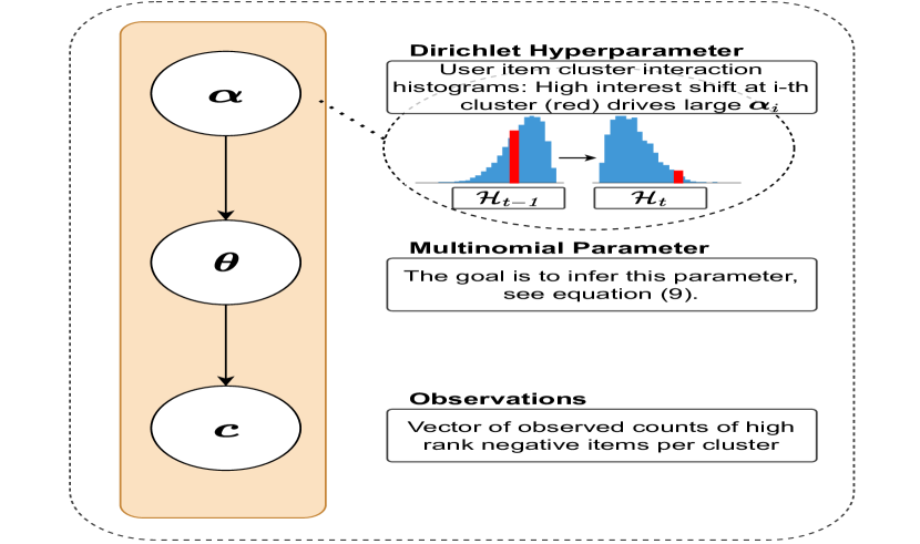
Figure 2. The hierarchical model in (10), (5.2). From time $t-1$ to $t$, the user loses interest in the i-th category, this increases $\bm{\alpha}_{i}$. This gives $\bm{\theta}_{i}$ a high prior value, thus we sample negatives with higher probability from that item category in (14).

We can then estimate $\bm{\theta}$ as the mean of the posterior:

(13) $$\bm{\hat{\theta}}_{i}=\mathbb{E}[\mathbf{\theta}_{i}\mid\mathbf{c}_{u,t,i}] =\frac{\lambda Q\operatorname{\textsc{softmax}}\bigg{(}\frac{\mathbf{H}_{u,t,i}}{|\mathbf{H}_{u,t,i}|}-\frac{\mathbf{H}_{u,t-1,i}}{|\mathbf{H}_{u,t-1,i}|}\bigg{)}+\mathbf{c}_{u,t,i}}{\sum_{i}\lambda Q\operatorname{\textsc{softmax}}\bigg{(}\frac{\mathbf{H}_{u,t,i}}{|\mathbf{H}_{u,t,i}|}-\frac{\mathbf{H}_{u,t-1,i}}{|\mathbf{H}_{u,t-1,i}|}\bigg{)}+\mathbf{c}_{u,t,i}}$$

Sampler for Reservoir: Denote $\bm{\hat{\theta}}_{u,t,C}$ as the $C$-th entry of $\bm{\hat{\theta}}_{u,t}$ ($C\in\{1,\dots,K\}$ is the item category that $i$ belongs to). Now, to sample negative items from the reservoir, we define the following sampler that draws negative item $n_{i}\in\mathcal{I}$ according to:

(14) $$p(n_{i}=i\mid i\in C,u,\bm{\hat{\theta}}_{u,t})\vcentcolon=\frac{\mathbb{I}_{[i\in\mathcal{Q}]}(i)\bm{\hat{\theta}}_{u,t,C}}{\sum_{i}\mathbb{I}_{[i\in\mathcal{Q}]}(i)\bm{\hat{\theta}}_{u,t,C}},$$

where and $\mathbb{I}_{[i\in\mathcal{Q}]}(i)$ is an indicator function that is one when item $i$ belongs to the set $\mathcal{Q}$ of top negative items for user $u$ at time $t$. Connecting this to the derivation in Section 5.1, vector $(N_{u,1},\dots,N_{u,|\mathcal{I}|})$ from (5.1) is a draw from the multinomial with parameters defined in (14).

Algorithm 1 Updating the Graph-SANE Reservoir

1:$\mathcal{R}_{t}\in\mathbb{R}^{|\mathcal{U}|\times|\mathcal{Q}|}$ $\triangleright$ top neg. items per user

2:$\mathbf{H}_{t},\mathbf{H}_{t-1}\in\mathbb{N}^{|\mathcal{U}|\times K}$ $\triangleright$ histogram of user-item category interactions at times $t$, $t-1$

3:$\mathbf{C}_{t}\in\mathbb{R}^{|\mathcal{I}|\times K}$ $\triangleright$ item to category one-hot map at time $t$

4:$\mathbf{M}_{t}\in\mathbb{R}^{|\mathcal{U}|\times|\mathcal{Q}|}\leftarrow 0$ $\triangleright$ stores probability of sampling neg. item $i$ for user $u$

5:for $u=0;u\leq|\mathcal{U}|;u++$ do

6:     for $i=0;i\leq|\mathcal{Q}|;i++$ do

7:         $\bm{\hat{\theta}}_{u,t}\in\mathbb{R}^{K}\leftarrow$ update sampling params from eq. (13)

8:         $C\leftarrow\operatorname*{arg\,max}\mathbf{C}_{t}[i,:]$ $\triangleright$ get category $i$ belongs to

9:         $\mathbf{M}_{t}[u,i]\leftarrow p(n_{i}=i|i\in C,\bm{\hat{\theta}}_{u,t})$ $\triangleright$ from eq. (14)

10:     end for

11:end for

5.3. Clustering

Recall that we often do not have attributes that can clearly identify item categories that could be used for clustering items into distinct interest groups. We overcome this problem by defining item pseudo-categories based on item clusters. The deep structural clustering method we use is adapted from two recent works by Bo et al. (Bo et al., 2020) and Wang et al. (Wang et al., 2019b). We select this method as the clusters are learned using both node attributes, the graph adjacency and because it is simple to adapt to our setting in an end-to-end trainable fashion.

For item $i$, we use the kernel of the Student’s t-distribution as a similarity measure between the item representation at time $t$, $\mathbf{h}^{t}_{i}$, and the $j$-th cluster centroid $\bm{\mu}_{k}^{t}$:

(15) $$q_{i,k}^{t}=\frac{(1+||\bm{h}_{i}^{t}-\bm{\mu}_{k}^{t}||^{2}/\nu)^{-\frac{\nu+1}{2}}}{\sum_{k^{\prime}\in K}(1+||\bm{h}_{i}^{t}-\bm{\mu}_{k^{\prime}}^{t}||^{2}/\nu)^{-\frac{\nu+1}{2}}}\,,$$

where $K$ is the total number of item clusters and $\nu$ represents the degrees of freedom of the distribution. We consider $q_{i,k}^{t}$ to be the probability of assigning item $i$ to cluster $k$. Then, $Q_{i}^{t}=[q_{i,1}^{t},\dots,q_{i,K}^{t}]$ is a discrete probability mass function that summarizes the probability of item $i$ belonging to each cluster at time $t$. The assignment of all items can be described by $Q^{t}=[q^{t}_{i,k}]$ To obtain confident cluster assignments we define $p$, a “sharpened” transformation of $q$:

(16) $$p_{i,k}^{t}=\frac{{(q_{i,k}^{t})^{2}}/\sum_{i}q_{i,k}^{t}}{\sum_{k^{\prime}}{(q_{i,k^{\prime}}^{t})^{2}}/\sum_{i}q_{i,k^{\prime}}^{t}}.$$

Then $P^{t}$ consists of the elements of $Q^{t}$ after being transformed by a square and normalization operation. By minimizing the Kullback–Leibler (KL) divergence (Kullback and Leibler, 1951) between $P^{t}$ and $Q^{t}$, we encourage more concentrated assignment to clusters.

(17) $$\mathcal{L}_{\textsc{KL}}=D_{\textsc{KL}}(\textsc{P}^{t}\mid\mid\textsc{Q}^{t})=\sum_{i}\sum_{m}p_{i,j}^{t}\log\frac{p_{i,j}^{t}}{q_{i,j}^{t}}.$$

In practice we first initialize $\bm{\mu}_{1},\bm{\mu}_{2},\dots,\bm{\mu}_{K}$ via K-means and then optimize (17) in subsequent training iterations so that the centroids are updated via back-propagation based on the gradients of $\mathcal{L}_{\textsc{KL}}$. We then model the probability of item $i$ belonging to cluster $k$ using $p_{i,k}^{t}$ by applying a softmax function with temperature $\tau\in\mathbb{R}_{+}$:

(18) $$\mathbf{c}_{i,k}^{t}=\frac{\text{exp}(\mathbf{p}_{i,k}^{t})/\tau}{\sum_{\hat{k}}\text{exp}(\mathbf{p}^{t}_{i,\hat{k}})/\tau}.$$

5.4. Overall Framework

In the previous subsections we detailed the design of the proposed negative reservoir that is sampled based on user change of preferences, and described the deep structural clustering procedure. In this section we present the overall objective function as well as providing an algorithm that summarizes our proposed incremental training framework. We emphasize that our proposed framework facilitates end-to-end training with any GNN backbone and any incremental learning framework. This includes both knowledge distillation and reservoir replay techniques.

While training using hard negative items can help improve gradient magnitudes and speed up convergence, it can cause instability (Ying et al., 2018a). To address this we use two sources of negative samples, hard negatives from our proposed reservoir as well as randomly selected negatives. The randomly selected negatives introduce diversity of samples as well as improving stability by moderating the effects of large gradient values obtained from hard negatives during the initial epochs (Ying et al., 2018a). The proposed objective function is:

(19) $$\mathcal{L}_{\textsc{Total}}=\beta_{1}\underbrace{\mathcal{L}_{\textsc{BASE}}}_{\text{$\mathcal{L}_{\textsc{BPR}},\mathcal{L}_{\textsc{KD}}$}}+\quad\beta_{2}\underbrace{\mathcal{L}_{\textsc{SANE}}}_{\text{Neg. Reservoir}}+\quad\beta_{3}\underbrace{\mathcal{L}_{\textsc{KL}}}_{\text{Cluster}},$$

where $\mathcal{L}_{\textsc{BASE}}$ consists of the base incremental learning model loss components, the knowledge distillation loss $\mathcal{L}_{\textsc{KD}}$ and the BPR loss $\mathcal{L}_{\textsc{BPR}}$ of the randomly sampled negatives, $\mathcal{L}_{\textsc{SANE}}$ is our proposed loss from the hard negative reservoir, $\mathcal{L}_{\textsc{KL}}$ is the KL loss component for the clustering and the weighting terms $\beta_{1},\beta_{2},\beta_{3}$ are used to balance the contribution of the loss components. In practice, we set $\beta_{1}=\beta_{2}=1$ and adjust $\beta_{3}$ so that the scaled KL loss term’s contribution does not dominate the overall loss. The training process with our method is detailed in Algorithm 2.

Algorithm 2 Incremental Training with Graph-SANE Reservoir

1:$\Theta_{t-1}$ $\triangleright$ params of model from block $t-1$

2:$f$, max_epochs $\triangleright$ refresh rate of reservoir, max epochs

3:$\mathcal{R}_{t}\in\mathbb{R}^{|\mathcal{U}|\times|\mathcal{Q}|}$ $\triangleright$ SANE reservoir

4:$N_{1},N_{2}$ $\triangleright$ num. random negatives, reservoir samples

5:$\textsc{n\_iter}\leftarrow 0$

6:repeat

7:     if $\textsc{n\_iter}\mod f==0$ then

8:         Update item cluster memberships using eq. (18)

9:         Update $\mathcal{R}_{t}$ using Algorithm 1

10:     end if

11:     Draw a batch of incremental data $\mathcal{B}\subseteq\{(u,i)\in\mathcal{E}_{[t-1,t)}\}$

12:     Draw $N_{1}$ random negatives $\mathcal{I}_{u}^{-}$

13:     Sample $N_{2}$ reservoir negatives $\mathcal{I}_{u}^{*-}$

14:     Compute loss components from eq. (19)

15:     Update parameters $\Theta$

16:     $\textsc{n\_iter}\leftarrow\textsc{n\_iter}+1$

17:until convergence

6. Experiments

This section empirically evaluates the proposed method GraphSANE. Our discussion is centered on the following research questions (RQ):

• RQ1 How does our method compare to standard SOTA incremental learning methods?

• RQ2 Is our proposed sampler better than generic negative samplers specifically in the incremental learning setting?

• RQ3 How does the time complexity of our sampler compare to other samplers? Is our approach scalable?

• RQ4 Where are the performance gains coming from? For which users does our method improve item recommendation?

• RQ5 How sensitive is the model to the clustering algorithm?

6.1. Datasets

We evaluate our proposed method empirically on five mainstream recommender system datasets. These datasets vary significantly in the total number of interactions, sparsity, average item and user node degrees as well as the time span they cover. Detailed dataset statistics are provided in Table 1. To simulate an incremental learning setting, the datasets are separated to 60% base blocks and four incremental blocks each with 10% of the remaining data. The splits are in chronological order. Fig. 1 depicts the data split per block.

Table 1. Statistics of the five datasets used in the experiments.

Gowalla Yelp Taobao2014 Taobao2015 Netflix # edges 281412 942395 749438 1332602 12402763 # users 5992 40863 8844 92605 63691 Avg. user degrees 46.96 23.06 84.74 14.39 194.73 # items 5639 25338 39103 9842 10271 Avg. item degrees 49.90 37.19 19.17 135.40 1207.56 Avg. % new users 2.67 3.94 1.67 2.67 4.36 Avg. % new items 0.67 1.72 2.60 0.22 0.72 Time span (months) 19 6 1 5 6

Table 2. Comparison (Recall@20) of baselines and 3 recent knowledge distillation algorithms with our SANE reservoir, our methods are accompanied by a star (*).

Yelp
Fine Tune	0.0705	0.0638	0.0640	0.0661	0.00
LSP_s	0.0722	0.0661	0.0644	0.0676	2.27
Uniform	0.0718	0.0635	0.0610	0.0654	-1.05
Inv_degree	0.0727	0.0699	0.0605	0.0677	2.42
GraphSAIL	0.0674	0.0617	0.0625	0.0639	-3.33
GraphSAIL-SANE*	0.0939	0.0842	0.0791	0.0857	29.7
SGCT	0.0740	0.0656	0.0608	0.0668	1.06
SGCT-SANE*	0.0966	0.0877	0.0744	0.0862	30.4
LWC-KD	0.0739	0.0661	0.0637	0.0679	2.72
LWC-KD-SANE*	0.0970	0.0891	0.0834	0.0898	35.9
Taobao14
Fine Tune	0.0208	0.0112	0.0138	0.0153	0.00
LSP_s	0.0213	0.0106	0.0138	0.0152	-0.65
Uniform	0.0195	0.0127	0.0148	0.0157	2.61
Inv_degree	0.0228	0.0140	0.0159	0.0175	14.63
GraphSAIL	0.0222	0.0105	0.0139	0.0155	1.31
GraphSAIL-SANE*	0.0231	0.0131	0.0150	0.0171	11.8
SGCT	0.0240	0.0092	0.0148	0.0160	1.74
SGCT-SANE*	0.0224	0.0136	0.0173	0.0178	16.3
LWC-KD	0.0254	0.0119	0.0156	0.0176	15.3
LWC-KD-SANE*	0.0222	0.0188	0.0155	0.0188	22.9
Taobao15
Fine Tune	0.0933	0.0952	0.0965	0.0950	0.00
LSP_s	0.0993	0.0952	0.0957	0.0968	1.86
Uniform	0.0988	0.0954	0.1004	0.0982	3.37
Inv_degree	0.0991	0.0977	0.1000	0.0989	4.16
GraphSAIL	0.0959	0.0959	0.0972	0.0963	1.39
GraphSAIL-SANE*	0.1114	0.1087	0.1121	0.1107	16.5
SGCT	0.1030	0.0983	0.0984	0.0999	5.16
SGCT-SANE*	0.1117	0.1129	0.1138	0.1128	18.7
LWC-KD	0.1039	0.1022	0.1029	0.1030	8.42
LWC-KD-SANE*	0.1106	0.1108	0.1128	0.1114	17.2
Netflix
Fine Tune	0.1092	0.1041	0.0977	0.1036	0.00
LSP_s	0.1173	0.1136	0.1076	0.1128	8.88
Uniform	0.1018	0.1055	0.0800	0.0957	-7.63
Inv_degree	0.1000	0.1050	0.0820	0.0957	-7.63
GraphSAIL	0.1163	0.1023	0.0968	0.1051	1.45
GraphSAIL-SANE*	0.1153	0.1091	0.01014	0.1086	4.82
SGCT	0.1166	0.1161	0.1077	0.1135	9.56
SGCT-SANE*	0.1182	0.1164	0.1120	0.1155	11.48
LWC-KD	0.1185	0.1170	0.1071	0.1142	10.23
LWC-KD-SANE*	0.1178	0.1189	0.1109	0.1182	14.09

Table 3. Comparison (Recall@20) of baselines and 3 recent knowledge distillation algorithms with our SANE reservoir, our methods are accompanied by a star (*).

Gowalla
Methods	Inc 1	Inc 2	Inc 3	Avg.	Imp %
Fine Tune	0.1412	0.1637	0.2065	0.1705	0.00
LSP_s	0.1512	0.1741	0.2097	0.1783	4.57
Uniform	0.1480	0.1653	0.2051	0.1728	1.34
Inv_degree	0.1483	0.1680	0.2001	0.1738	1.93
GraphSAIL	0.1529	0.1823	0.2195	0.1849	8.44
GraphSAIL-SANE*	0.1646	0.1907	0.2221	0.1925	12.9
SGCT	0.1588	0.1815	0.2207	0.1870	9.68
SGCT-SANE*	0.1611	0.1843	0.2237	0.1897	11.3
LWC-KD	0.1639	0.1921	0.2368	0.1977	15.9
LWC-KD-SANE*	0.1698	0.1835	0.2173	0.1881	10.3

6.2. Baselines

Our base model recommendation system is MGCCF (Sun et al., 2019), a commonly used architecture in the incremental recommendation setting ( (Xu et al., 2020; Wang et al., 2021b)) that is specifically designed to handle bipartite graphs. All the incremental learning algorithms are built on top of this backbone model. In our first set of experiments summarized in Table 2, we evaluate our model in comparison to multiple baselines, including the current SOTA graph incremental learning approaches.

Fine Tune: Fine-tune naively trains on new incremental data of each time block to update the model that was trained using the previous time block’s data. It is prone to “catastrophic forgetting”.

LSP_s (Yang et al., 2020): LSP is a knowledge distillation technique tailored to Graph Convolution Network (GCN) models.

Uniform: This method randomly samples and replays a subset of old data along with the incremental data to alleviate forgetting.

Inv_degree (Ahrabian et al., 2021): Inv_degree is a state-of-art reservoir replay method. The reservoir is constructed from historical user-item interactions. The inclusion probability of an interaction is proportional to the inverse degree of the user.

SOTA Graph Rec. Sys. Incremental Learning methods: GraphSail (Xu et al., 2020), SGCT (Wang et al., 2021b) and LWC-KD (Wang et al., 2021b) are state-of-the-art knowledge distillation techniques. We integrate our design into these SOTA models and compare to see if this improves upon them.

In the second set of experiments, we investigate if our user interest shift aware negative reservoir design tailored specifically for incremental learning is effective compared to alternative designs. We investigate how several prominent existing negative sampling strategies perform in incremental learning.

WARP (Weston et al., 2010): This method randomly samples negatives samples from the pool of unobserved interactions.

Popularity-based Negative Sampling (PNS) (Rendle and Freudenthaler, 2014b): This method ranks the top negatives and samples them with a fixed parametric distribution, e.g., a geometric.

PinSage Sampler (Ying et al., 2018a): This negative sampler ranks items based on personalized PageRank and then samples high rank negatives. Note, this is not to be confused with the overall PinSage GNN recommender system backbone — we merely use the negative sampler.

Negative Sample Caching (NS Cache) (Zhang et al., 2019): This is a knowledge graph negative sampler which we adapt to our setting. It samples negative items and compares them to cache content. The negative samples randomly replace cached entries proportionally to their likelihood following an importance sampling approach. This algorithm has fewer parameters than GAN-based negative samplers, such as KGAN (Cai and Wang, 2018) and IGAN (Wang et al., 2018). Besides, it is fully trainable using back-propagation and has equal or better performance than GAN-based methods.
Hyperparameters and Reproducibility We make our experimental code available For completeness we list some key hyperparameters here: The training loop is implemented in TensorFlow using Adam (Kingma and Ba, 2015) with a learning rate of 5e-4 and batch size of 64. We use 2 GNN layers in the MGCCF model with an embedding dimension of 128 and update the reservoir every two epochs.

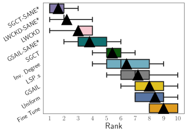
Figure 3. Boxplot of ranks of the algorithms across the 5 datasets. The medians and means of the ranks are shown by the vertical lines and the black triangles respectively; whiskers extend to the minimum and maximum ranks. Stars “*” represent methods that integrate our proposed negative reservoir. We abbreviate GraphSail to “GSAIL”.

6.3. Comparison to SOTA Inc. Learning (RQ1)

Our first set of experiments compares our method to the standard incremental learning baselines on five mainstream datasets. We use the exact same base MGCCF (Sun et al., 2019) backbone model instance trained on the base block for all incremental learning methods. We integrate our negative reservoir design SANE in three SOTA and commonly used incremental recommendation models, including GraphSAIL (Xu et al., 2020), SGCT (Wang et al., 2021b), and LWC-KD (Wang et al., 2021b). The experiment convincingly demonstrates the value of considering a negative reservoir in conjunction with standard incremental learning approaches. We show in Table 2 that our method strongly outperforms for almost all datasets, achieving top performance in all but the smallest dataset in Tab. 3. This is not unexpected since the smallest dataset, Gowalla has only $\sim 5000$ items. With an average user degree of $\sim 50$ and assuming we select 10 negative samples per observed interaction for the optimization we observe that randomly sampling the negatives without replacement yields a negative sample size that is approximate $50\times 10/5000=10\%$ of the total item population per epoch. Training for 10-20 epochs virtually guarantees that the pool of all potential negatives will be exhausted, thus reducing the effectiveness of any non-trivial negative sampler relative to brute force sampling of all the negatives. On moderate and large datasets our method is the top performer by a convincing margin, often offering more than 10% improvement compared to the top-performing baselines that do not use our negative reservoir. Overall, our designed negative reservoir can boost the average performance of three SOTA incremental learning frameworks, GraphSAIL, SGCT, and LWC-KD by 13.4%, 9.4% and 6.7%, respectively, across five datasets. Furthermore, as summarized in Fig. 3, SGCT-SANE is the top-performing method when comparing all the alternatives.

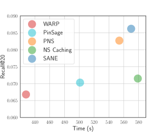
Figure 4. Comparison of recall performance and training time required per incremental block for various negative samplers of Yelp discussed in Table 4. As we can see our proposed reservoir method outperforms with time complexity in line with the baselines. Note that full batch retraining takes more than an hour per block.

Table 4. Comparison of mainstream negative samplers with our proposed reservoir in terms of Recall@20.

Dataset Methods Inc 1 Inc 2 Inc 3 Avg. Yelp SGCT+[Warp] 0.0740 0.0656 0.0608 0.0668 SGCT+[PinSage] 0.0794 0.0663 0.0651 0.0703 SGCT+[PNS] 0.0933 0.0798 0.0748 0.0827 SGCT+[NS Cache] 0.0794 0.0681 0.0670 0.0715 SGCT+[SANE] (ours) 0.0966 0.0877 0.0744 0.0862 Taobao14 SGCT+[Warp] 0.0240 0.0092 0.0148 0.0160 SGCT+[PinSage] 0.0241 0.0099 0.0151 0.0164 SGCT+[PNS] 0.0220 0.0114 0.0113 0.0149 SGCT+[NS Cache] 0.0237 0.0124 0.0121 0.0165 SGCT+[SANE] (ours) 0.0224 0.0136 0.0173 0.0178

6.4. More Metrics: Precision, MAP, NDCG (RQ1)

In the previous subsection and Table 2 we only presented Recall@20 metrics. Here, we present a summary of the results of the same experimental setup as in Table 2 and Fig. 3 but also include results for Precision@k, mean average precision (MAP@k) and normalized discounted cumulative gain (NDCG@k). We show results that depict the overall rank of the methods, averaged across the datasets for $k=20$. We ran experiments for $k\in\{5,10,15,20\}$ and obtained very similar results to Table 5 in all cases. Our results span 5 datasets, 4 distinct $k$ values for 4 different metrics and pairwise comparison of 3 incremental models (using our reservoir versus not using it). This yields $5\times 4\times 4\times 3=240$ distinct comparisons. Our method improves upon the baseline in 178/240 (74.2%) of the cases, and the improvement is larger than 5% in 157/240 (65.4%) of the cases. We note that the majority of the cases where our model does not improve upon the base model is in Gowalla-20, which as explained earlier is a pathological case. If we exclude Gowalla-20, our model improves the base models $\sim$85% of the time.

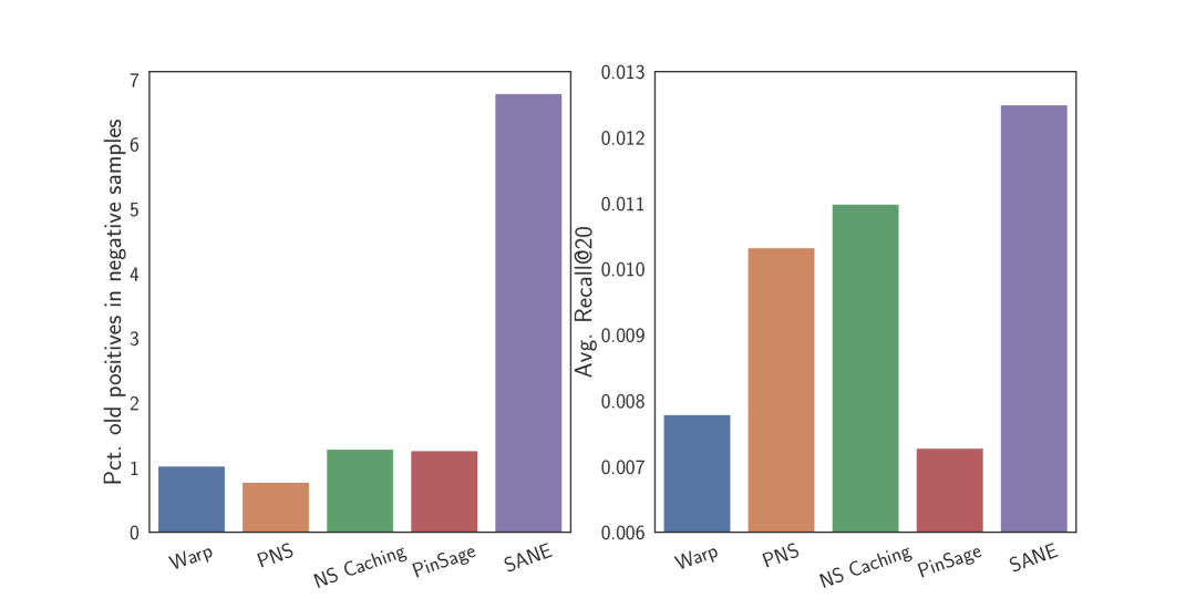
Figure 5. Case Study: Among the 15% of users with highest interest shift on Taobao14 we observe that Graph-SANE increases the amount of old positives sampled as current negatives by 7 times. Our sampler strongly improves Recall@20.

Table 5. Average ranks of models for key metrics across Gowalla, Yelp, Taobao14, Taobao15. Lower rank is better ($\downarrow$). Bold indicates improvement over base model.

Recall@20 Rank ($\downarrow$) NDCG@20 Rank ($\downarrow$) Precision@20 Rank ($\downarrow$) MAP@20 Rank ($\downarrow$) GraphSail 6.00 4.75 5.00 5.00 GraphSail+SANE 3.00 3.75 3.25 3.50 SGCT 4.75 4.75 4.50 4.50 SCGT+SANE 1.50 2.00 3.25 2.00 LWCKD 3.25 3.25 1.75 3.25 LWCKD+SANE 2.25 2.75 3.50 2.50

6.5. Comparison to Generic Neg. Samplers (RQ2)

Our second experiment focuses on evaluating the proposed negative sampler for the reservoir. The goal of this experiment is to demonstrate the effectiveness of our negative sampler in the context of incremental learning. For the baselines, we replace $\mathcal{L}_{\textsc{SANE}}$ with a standard triplet loss, i.e., BPR, and draw the negatives according to the baseline negative sampler algorithms. We select one incremental learning framework, SGCT, replicate the same incremental learning setup for Yelp and Taobao2014 and vary the choice of negative samplers. As shown in Table 4, our method offers a consistent performance improvement. We conjecture that the performance gain arises because our sampler is the only one that is designed explicitly for the incremental setting, rather than being designed for a static setting and then adapted (this is investigated in the case study in the subsequent section). We compare the performance and the time to train one incremental block of Yelp for different samplers in Fig. 4. The proposed approach takes approximately the same amount of time as PNS and NS Caching and roughly 20% more time than the vanilla WARP.

6.6. Time Complexity & Efficient Scaling (RQ3)

For training complexity the main cost comes from ranking the items. Our approach exploits the fact that in a real world setting recommender systems that are trained incrementally start with a rank of the items from the previous data block. We only need to rank the items 2-3 times as the number of training epochs until model convergence is usually very low (between 5-15) for all of our datasets, even though they vary in size dramatically. Therefore, the computational cost of ranking the items a handful of times is not unreasonable. Inference time is not affected by our algorithm as we do not cluster or sample negatives during model evaluation.

BPR (Rendle et al., 2009) and WARP (Zhao et al., 2015) select negatives at random so they are the most efficient. The PinSage sampler (Ying et al., 2018b) requires running a personalized PageRank algorithm to rank the items, assuming that the incremental block data do not radically change the graph topology the PageRank iterations should converge quickly if the previous block’s PageRank vector is used as an initial guess to the iterative PageRank algorithm. Score and rank based models require computing dot products between user and item embeddings which costs $O(|\mathcal{U}||\mathcal{I}|)$. These are typically the most expensive models but often to lead to “hard” negatives that can significantly improve training convergence. Such methods include our method as well as (Zhang et al., 2019; Rendle and Freudenthaler, 2014a; Zhang et al., 2013). In general, ranking all the items incurs a computational cost of $O(|\mathcal{U}||\mathcal{I}|\log(|\mathcal{I}|)$. We note that we only rank the top $|\mathcal{Q}|$ items which further reduces the complexity to $O(|\mathcal{U}||\mathcal{I}|)$ on the average case using the QuickSelect algorithm (Hoare, 1961). Since each user’s item ranks are independent of all the other users the embedding dot products and ranking can be done in parallel.

6.7. Case Study: GraphSANE Improves Recommendation for Dynamic Users (RQ4)

We conduct a case study on Taobao14 on the users with high preference shift to investigate their negative items drawn from the various samplers. Since our approach aims to model user interest shift we expect our model to (i) draw more negatives from the clusters that users were previously interested in but not anymore in current time block, including old positive items and (ii) outperform in the recall metric since this is the main subset of users that our algorithm focuses on. As we can see in Fig. 5, our algorithm increases the proportion of negative samples from old positives by sevenfold and offers clear improvement of about 20% in Recall@20. Details for the case study are available in Appendix A.

6.8. Clustering Algorithm Sensitivity (RQ5)

Table 6. Sensitivity to clustering algorithm choice in Yelp.

Methods Inc. 1 Inc. 2 Inc.3 Avg. GraphSAIL+SANE (K-means) 0.0877 0.0871 0.0791 0.0846 GraphSAIL+SANE (end-to-end - ours) 0.0939 0.0842 0.0791 0.0857 SGCT+SANE (K-means) 0.0946 0.0858 0.0732 0.0845 SGCT+SANE (end-to-end - ours) 0.0966 0.0877 0.0744 0.0857 LWC-KD+SANE (K-means) 0.0931 0.0853 0.0787 0.0857 LWC-KD+SANE (end-to-end - ours) 0.0924 0.0855 0.0798 0.0859

In this ablation study we check if an ad-hoc training scheme where we cluster the items using K-means between epochs can produce similar results to our approach, which uses an end-to-end structural based clustering method (Bo et al., 2020). In Table 8 observe that our method performs within 1-3% with either clustering algorithm, thus validating the low sensitivity towards clustering algorithm selection. We obtain similar results when we vary the dataset choice and the number of clusters. The attributed clustering algorithm maintains end-to-end trainability so it converges faster than K-means.

7. Conclusion

This work proposes a novel incremental learning technique for recommendation systems to sample the negatives in the triplet loss. Our approach is easy to implement on top of any graph-based recommendation system backbone such as PinSage(Ying et al., 2018a), MGCCF (Sun et al., 2019) or LightGCN (He et al., 2020) and can be easily combined with base incremental learning methods. When used in conjunction with standard knowledge distillation approaches, our method demonstrates a very strong improvement over the current state-of-the-art models.

Appendix

Appendix A Case Study Details

To conduct this case study we chose a clustering algorithm that differs from the one used in our method. This is done to provide an alternative estimate of high shift users that is not part of our model. Note that the the user shift indicator, i.e. the technique to identify high interest shift users, we use follows the process introduced by Wang et al. (Wang et al., 2023). For completeness we explicitly list the steps taken by Wang et al. (Wang et al., 2023):

1. Apply K-means on item embeddings at time block $t$ obtained from the SGCT model to identify $K$ clusters.

2. Obtain $\tilde{\bm{I}}^{t}\in\mathbb{R}^{U\times K}$ by counting number of items from each category a user interacts with for all $t$.

3. Normalize $\tilde{\bm{I}^{t}}$ to calculate $\bm{I}_{k}=\tilde{\bm{I}^{t}}_{k}/\sum_{k^{\prime}\in K}\tilde{\bm{I}^{t}}_{k}^{\prime}$.

4. Obtain interest shift indicator: $ISS_{u}=\frac{1}{K}\sum_{k=1}^{K}||\bm{I}^{t}_{u,k}-\bm{I}^{t-1}_{u,k}||^{2}$.

5. We define users with top 15% interest shift indicator as the high shift user set.

6. Calculate average recall for the high shift users using all the different negative samplers on top of SGCT.

Appendix B Loss Ablation Study & Sensitivity Analysis

In this section we conduct a loss ablation study on our proposed objective, as well as sensitivity studies on key components of our method: the choice of specific clustering algorithm, the number of clusters of our clustering algorithm as well as the size of our proposed negative reservoir. The dataset choice for the ablation and sensitivity experiments can be explained by the fact that Netflix, which is our biggest dataset, is prohibitvely big to run many experiments on as it takes over 2 days per experiment (see runtime section), so we opt for Yelp and Taobao14 as they have the most representative number of user and items compared to the average dataset (they are neither the biggest nor the smallest).

Our loss ablation study validates each term in the proposed loss. Concretely, we check the impact of removing each loss term from our overall proposed optimization objective. As we can see in Tables 11 and 12 removing any of our proposed components impacts performance and/or end-to-end trainability.

In the first sensitivity study we investigate if an ad-hoc training scheme where we cluster the items using K-means between epochs can produce similar results to our approach, which uses an end-to-end structural based clustering method (Bo et al., 2020). In Tables 7, 8 we observe that our method performs within 1-3% with either clustering algorithm, thus validating the low sensitivity towards clustering algorithm selection. We obtain similar results when we vary the dataset choice and the number of clusters. The attributed clustering algorithm maintains end-to-end trainability so it converges faster than K-means.

Table 7. Sensitivity to clustering algorithm choice in Yelp. Results demonstrate low sensitivity to specific algorithm choice.

Methods Inc. 1 Inc. 2 Inc.3 Avg. GraphSAIL+SANE (K-means) 0.0877 0.0871 0.0791 0.0846 GraphSAIL+SANE (end-to-end - ours) 0.0939 0.0842 0.0791 0.0857 SGCT+SANE (K-means) 0.0946 0.0858 0.0732 0.0845 SGCT+SANE (end-to-end - ours) 0.0966 0.0877 0.0744 0.0857 LWC-KD+SANE (K-means) 0.0931 0.0853 0.0787 0.0857 LWC-KD+SANE (end-to-end - ours) 0.0970 0.0891 0.0834 0.0898

Table 8. Sensitivity to clustering algo. choice in Taobao14. Results demonstrate low sensitivity to specific algorithm choice.

Methods Inc. 1 Inc. 2 Inc.3 Avg. GraphSAIL+SANE (K-means) 0.0222 0.0139 0.0165 0.0175 GraphSAIL+SANE (end-to-end) 0.0231 0.0131 0.0150 0.0171 SGCT+SANE (K-means) 0.0228 0.0154 0.0153 0.0178 SGCT+SANE (end-to-end) 0.0224 0.0136 0.0173 0.0178 LWC-KD+SANE (K-means) 0.0228 0.0174 0.0154 0.0185 LWC-KD+SANE (end-to-end) 0.0222 0.0188 0.0156 0.0188

In the second sensitivity study, shown in Table 9, we conduct an analysis on the number of clusters used in our method. As we can see, once the number of clusters reaches a sufficient number $\sim 10$, the performance remains stable.

Table 9. Sensitivity analysis for the cluster number K. We present Recall@20 results on the Gowalla and Taobao2015 datasets for SGCT-SANE and LWC-KD-SANE. Results demonstrate low sensitivity to number of clusters.

Distillation Strategies	Dataset	K	Inc 1	Inc 2	Inc 3	Avg. Recall@20
Taobao14	SGCT-SANE	5	0.0240	0.0133	0.0127	0.0167
		10	0.0224	0.0136	0.0173	0.0178
		15	0.0237	0.0143	0.0143	0.0174
		20	0.0237	0.0154	0.0165	0.0185
		25	0.0234	0.0156	0.0166	0.0185
	LWC-KD-SANE	5	0.0265	0.0121	0.0150	0.0179
		10	0.0222	0.0188	0.0155	0.0188
		15	0.0251	0.0138	0.0161	0.0183
		20	0.0247	0.0128	0.0145	0.0173
		25	0.0247	0.0141	0.0162	0.0183

Thirdly, in Table10, we conduct a sensitivity analysis on the size of the user negative reservoir $\lvert\mathcal{Q}\lvert$. As we can see, the method is not sensitive to the size of the reservoir. This implies that introducing even a few hard negatives in the incremental training can be sufficient to improve performance.

Table 10. Sensitivity analysis on the size of the user negative reservoir $\lvert\mathcal{Q}\lvert$. We present Recall@20 results on the Gowalla and Taobao2015 datasets for SGCT-SANE and LWC-KD-SANE. Results demonstrate low sensitivity to negative reservoir size.

Distillation Strategies	Dataset	$\lvert\mathcal{Q}\lvert$	Inc 1	Inc 2	Inc 3	Avg. Recall@20
Taobao14	SGCT-SANE	50	0.0237	0.0156	0.0160	0.0184
		100	0.0224	0.0136	0.0173	0.0178
		300	0.0254	0.0140	0.0160	0.0185
	LWC-KD-SANE	50	0.0238	0.0140	0.0162	0.0180
		100	0.0222	0.0188	0.0155	0.0188
		300	0.0246	0.0133	0.0180	0.0186

Table 11. Loss components ablation on Taobao14 and Yelp for SGCT-SANE (Recall@20). We check the impact of removing each loss term from our overall proposed optimization objective. As we can see, removing any of our proposed components impacts performance and/or end-to-end trainability.

Method	$\mathcal{L}_{\textsc{BPR}}$	$\mathcal{L}_{\textsc{KD}}$	$\mathcal{L}_{\textsc{SANE}}$	$\mathcal{L}_{\textsc{KL}}$	End-to-End Trainable	Taobao14	Yelp
Fine Tune	✓	✗	✗	✗	Yes	0.0153	0.0661
SGCT	✓	✓	✗	✗	Yes	0.0160	0.0668
SGCT-hard-cluster	✓	✓	✓	✗	No	0.0178	0.0845
SGCT-SANE (ours)	✓	✓	✓	✓	Yes	0.0178	0.0857

Table 12. Loss components ablation on Taobao14 and Yelp for LWCKD-SANE (Recall@20). As we can see, removing any of our proposed components impacts performance and/or end-to-end trainability.

Method	$\mathcal{L}_{\textsc{BPR}}$	$\mathcal{L}_{\textsc{KD}}$	$\mathcal{L}_{\textsc{SANE}}$	$\mathcal{L}_{\textsc{KL}}$	End-to-End Trainable	Taobao14	Yelp
Fine Tune	✓	✗	✗	✗	Yes	0.0153	0.0661
LWCKD	✓	✓	✗	✗	Yes	0.0176	0.0679
LWCKD-hard-cluster	✓	✓	✓	✗	No	0.0185	0.0857
LWCKD-SANE (ours)	✓	✓	✓	✓	Yes	0.0188	0.0898

Appendix C Hyperparameter Settings

Our method is implemented in TensorFlow.

Table 13. Hyperparameters of our model on all benchmarks.

Hyperparameter	Value
Min Epochs Base Block	10
Min Epochs Incremental	3
Max Epochs Base Block	N/A
Max Epochs Incremental	15
Early Stopping Patience	2
Batch size	64
Optimizer	Adam
Cache Update Frequency $f$	2 epochs
Cache Size per user $|\mathcal{Q}|$	100
Learning rate (max)	5e-4
Dropout	0.2
Losses	KD, BPR, SANE, KL
GNN Num Layers ($L$)	2
Num Clusters ($K$)	10
Embedding dimensionality	128
Augmentations	NONE

The backbone graph neural network is the MGCCF (Sun et al., 2019) trained using the hyperparameters shown in Table 13. Incremental learning methods are not used during the base block training so the loss during the base block is only $\mathcal{L}_{\textsc{BPR}}$, i.e., (no $\mathcal{L}_{\textsc{KD}}$, $\mathcal{L}_{\textsc{SANE}}$, $\mathcal{L}_{\textsc{KL}}$ components).

References

- (1)
- Ahrabian et al. (2021) Kian Ahrabian, Yishi Xu, Yingxue Zhang, Jiapeng Wu, Yuening Wang, and Mark Coates. 2021. Structure Aware Experience Replay for Incremental Learning in Graph-based Recommender Systems. In Proc. ACM Int. Conf. Info. & Knowledge Management (CIKM). 2832–2836.
- Bo et al. (2020) Deyu Bo, Xiao Wang, Chuan Shi, Meiqi Zhu, Emiao Lu, and Peng Cui. 2020. Structural Deep Clustering Network. In Proc. World Wide Web Conf. (WWW). 1400–1410.
- Cai and Wang (2018) Liwei Cai and William Yang Wang. 2018. KBGAN: Adversarial Learning for Knowledge Graph Embeddings. In Proc. Conf. N. American Chapter Assoc. Computational Linguistics. New Orleans, LA, USA.
- Caselles-Dupré et al. (2018) Hugo Caselles-Dupré, Florian Lesaint, and Jimena Royo-Letelier. 2018. Word2vec applied to recommendation: Hyperparameters matter. In Proceedings of the 12th ACM Conference on Recommender Systems. 352–356.
- Castro et al. (2018) Francisco M. Castro, Manuel J. Marín-Jiménez, Nicolás Guil, Cordelia Schmid, and Karteek Alahari. 2018. End-to-End Incremental Learning. In Proc. European Conf. Computer Vision (ECCV). 241–257.
- Cheng et al. (2016) Heng-Tze Cheng, Levent Koc, Jeremiah Harmsen, Tal Shaked, Tushar Chandra, et al. 2016. Wide & Deep Learning for Recommender Systems. In Proc. ACM Recommender Syst. Conf. - Workshop on Deep Learning for Recommender Syst. (Boston, MA, USA). 7–10.
- Covington et al. (2016) Paul Covington, Jay Adams, and Emre Sargin. 2016. Deep neural networks for youtube recommendations. In Proc. ACM Conf. Recommender Syst. 191–198.
- Fan et al. (2021) Ziwei Fan, Zhiwei Liu, Jiawei Zhang, Yun Xiong, Lei Zheng, and Philip S Yu. 2021. Continuous-time sequential recommendation with temporal graph collaborative transformer. In Proc. ACM Int. Conf. Info. & Knowledge Management (CIKM). 433–442.
- Guo et al. (2017) Huifeng Guo, Ruiming Tang, Yunming Ye, Zhenguo Li, and Xiuqiang He. 2017. Deepfm: a factorization-machine based neural network for ctr prediction. In Proc. Int. Joint. Conf. Artificial Intelligence (IJCAI). 1725–1731.
- He et al. (2020) Xiangnan He, Kuan Deng, Xiang Wang, Yan Li, Yong-Dong Zhang, and Meng Wang. 2020. LightGCN: Simplifying and Powering Graph Convolution Network for Recommendation. In SIGIR. ACM.
- He et al. (2023) Zhicheng He, Weiwen Liu, Wei Guo, Jiarui Qin, Yingxue Zhang, Yaochen Hu, and Ruiming Tang. 2023. A Survey on User Behavior Modeling in Recommender Systems. (2023).
- Hidasi and Karatzoglou (2018) Balázs Hidasi and Alexandros Karatzoglou. 2018. Recurrent neural networks with top-k gains for session-based recommendations. In Proc. ACM Int. Conf. Info. & Knowledge Management (CIKM). 843–852.
- Hinton et al. (2015) Geoffrey Hinton, Oriol Vinyals, and Jeff Dean. 2015. Distilling the Knowledge in a Neural Network. CoRR arXiv (2015).
- Hoare (1961) C. A. R. Hoare. 1961. Algorithm 65: Find. Commun. ACM 4, 7 (Jul. 1961), 321–322.
- Kang and McAuley (2018) Wang-Cheng Kang and Julian McAuley. 2018. Self-attentive sequential recommendation. In Proc. IEEE Int. Conf. Data Mining (ICDM). 197–206.
- Kingma and Ba (2015) Diederik P. Kingma and Jimmy Ba. 2015. Adam: A Method for Stochastic Optimization. CoRR abs/1412.6980 (2015).
- Kipf and Welling (2017) Thomas N. Kipf and Max Welling. 2017. Semi-Supervised Classification with Graph Convolutional Networks. In Proc. Int. Conf. Learning Representations (ICLR).
- Kirkpatrick et al. (2017) James Kirkpatrick, Razvan Pascanu, Neil Rabinowitz, Joel Veness, Guillaume Desjardins, Andrei A Rusu, Kieran Milan, John Quan, Tiago Ramalho, Agnieszka Grabska-Barwinska, et al. 2017. Overcoming catastrophic forgetting in neural networks. National Academy of Sciences 114, 13 (2017), 3521–3526.
- Kullback and Leibler (1951) S. Kullback and R. A. Leibler. 1951. On Information and Sufficiency. The Annals of Mathematical Statistics 22 (1951), 79 – 86.
- Prabhu et al. (2020) Ameya Prabhu, Philip HS Torr, and Puneet K Dokania. 2020. GDumb: A simple approach that questions our progress in continual learning. In European Conf. Computer Vision (ECCV). 524–540.
- Rebuffi et al. (2017) Sylvestre-Alvise Rebuffi, Alexander Kolesnikov, Georg Sperl, and Christoph H Lampert. 2017. iCarl: Incremental classifier and representation learning. In Proc. IEEE Conf. Computer Vision and Pattern Recognition. 2001–2010.
- Rendle and Freudenthaler (2014a) Steffen Rendle and Christoph Freudenthaler. 2014a. Improving pairwise learning for item recommendation from implicit feedback. In Proceedings of the 7th ACM international conference on Web search and data mining. 273–282.
- Rendle and Freudenthaler (2014b) Steffen Rendle and Christoph Freudenthaler. 2014b. Improving pairwise learning for item recommendation from implicit feedback. In Proc. Int. Conf. Web Search and Data Mining (WSDM). New York, NY, USA, 273–282.
- Rendle et al. (2009) Steffen Rendle, Christoph Freudenthaler, Zeno Gantner, and Lars Schmidt-Thieme. 2009. BPR: Bayesian Personalized Ranking from Implicit Feedback. In Proc. Conf. on Uncertainty in Artificial Intell. (UAI). Montreal, Canada, 452–461.
- Shmelkov et al. (2017) Konstantin Shmelkov, Cordelia Schmid, and Karteek Alahari. 2017. Incremental Learning of Object Detectors Without Catastrophic Forgetting. In Proc. Int. Conf. Computer Vision (ICCV). 3400–3409.
- Sun et al. (2019) Jianing Sun, Yingxue Zhang, Chen Ma, Mark Coates, Huifeng Guo, Ruiming Tang, and Xiuqiang He. 2019. Multi-Graph Convolution Collaborative Filtering. In Proc. IEEE Int. Conf. Data Mining (ICDM). 1306–1311.
- van den Berg et al. (2018) Rianne van den Berg, Thomas N. Kipf, and Max Welling. 2018. Graph Convolutional Matrix Completion. In ACM SIGKDD Int. Conf. Knowledge Discovery & Data Mining - Deep Learning Day Workshop.
- Wang et al. (2019b) Chun Wang, Shirui Pan, Ruiqi Hu, Guodong Long, Jing Jiang, and Chengqi Zhang. 2019b. Attributed Graph Clustering: A Deep Attentional Embedding Approach. In Proc. Int. Joint Conf. Artificial Intelligence (IJCAI) (Macao, China). 3670–3676.
- Wang et al. (2020) Junshan Wang, Guojie Song, Yi Wu, and Liang Wang. 2020. Streaming Graph Neural Networks via Continual Learning. In Proc. ACM Int. Conf. Info. & Knowledge Management. 1515–1524.
- Wang et al. (2017) Jun Wang, Lantao Yu, Weinan Zhang, Yu Gong, Yinghui Xu, Benyou Wang, Peng Zhang, and Dell Zhang. 2017. Irgan: A minimax game for unifying generative and discriminative information retrieval models. In Proc. Int. ACM SIGIR Conf. Research and Dev. Info. Retrieval. 515–524.
- Wang et al. (2018) Peifeng Wang, Shuangyin Li, and Rong Pan. 2018. Incorporating gan for negative sampling in knowledge representation learning. In Proc. Conf. Artificial Intell. (AAAI), Vol. 32.
- Wang et al. (2021a) Shoujin Wang, Liang Hu, Yan Wang, Xiangnan He, Quan Z Sheng, Mehmet A Orgun, Longbing Cao, Francesco Ricci, and Philip S Yu. 2021a. Graph learning based recommender systems: A review. In Proc. Int. Joint. Conf. Artificial Intelligence (IJCAI). 4644–4652.
- Wang et al. (2019a) Xiang Wang, Xiangnan He, Meng Wang, Fuli Feng, and Tat-Seng Chua. 2019a. Neural Graph Collaborative Filtering. In Proc. ACM Int. Conf. Research and Development in Info. Retrieval. 165–174.
- Wang et al. (2021b) Yuening Wang, Yingxue Zhang, and Mark Coates. 2021b. Graph Structure Aware Contrastive Knowledge Distillation for Incremental Learning in Recommender Systems. In Proc. ACM Int. Conf. Info. & Knowledge Management. 3518–3522.
- Wang et al. (2023) Yuening Wang, Yingxue Zhang, Antonios Valkanas, Ruiming Tang, Chen Ma, Jianye Hao, and Mark Coates. 2023. Structure Aware Incremental Learning with Personalized Imitation Weights for Recommender Systems. In Proc. AAAI Conf. Artificial Intelligence. 4711–4719.
- Weston et al. (2010) Jason Weston, Samy Bengio, and Nicolas Usunier. 2010. Large scale image annotation: learning to rank with joint word-image embeddings. Machine Learning 81 (2010), 21–35.
- Xu et al. (2020) Yishi Xu, Yingxue Zhang, Wei Guo, Huifeng Guo, Ruiming Tang, and Mark Coates. 2020. GraphSAIL: Graph Structure Aware Incremental Learning for Recommender Systems. In Proc. ACM Int. Conf. Info. & Knowledge Management. 2861–2868.
- Yang et al. (2020) Yiding Yang, Jiayan Qiu, Mingli Song, Dacheng Tao, and Xinchao Wang. 2020. Distilling Knowledge from Graph Convolutional Networks. In Proc. IEEE Conf. Computer Vision Pattern Recognition (CVPR). 7074–7083.
- Ying et al. (2018a) Rex Ying, Ruining He, Kaifeng Chen, Pong Eksombatchai, William L Hamilton, and Jure Leskovec. 2018a. Graph convolutional neural networks for web-scale recommender systems. In Proc. Int. Conf. Knowledge Discovery & Data Mining (KDD). London, UK, 974–983.
- Ying et al. (2018b) Rex Ying, Jiaxuan You, Christopher Morris, Xiang Ren, William L. Hamilton, and Jure Leskovec. 2018b. Hierarchical Graph Representation Learning with Differentiable Pooling. In Proc. Adv. Neural Inf. Process. Syst. (NeurIPS). Montréal, Canada, 4805–4815.
- Yu et al. (2022) Lu Yu, Shichao Pei, Feng Zhu, Longfei Li, Jun Zhou, Chuxu Zhang, and Xiangliang Zhang. 2022. A Biased Sampling Method for Imbalanced Personalized Ranking. In Proc. ACM Int. Conf. Info. Knowledge Management (CIKM) (Atlanta, GA, USA). 2393–2402.
- Zhang et al. (2013) Weinan Zhang, Tianqi Chen, Jun Wang, and Yong Yu. 2013. Optimizing top-n collaborative filtering via dynamic negative item sampling. In Proceedings of the 36th international ACM SIGIR conference on Research and development in information retrieval. 785–788.
- Zhang et al. (2019) Yongqi Zhang, Quanming Yao, Yingxia Shao, and Lei Chen. 2019. NSCaching: simple and efficient negative sampling for knowledge graph embedding. In IEEE Int. Conf. Data Engineering (ICDE). 614–625.
- Zhao et al. (2015) Tong Zhao, Julian McAuley, and Irwin King. 2015. Improving latent factor models via personalized feature projection for one class recommendation. In Proceedings of the 24th ACM international on conference on information and knowledge management. 821–830.