HELLO project: High-$z$ Evolution of Large and Luminous Objects

Abstract

We present the High-$z$ Evolution of Large and Luminous Objects (HELLO) project, a set of more than 30 high-resolution hydrodynamical cosmological simulations aimed to study Milky Way analogues ($M_{\star}\sim 10^{10-11}$ ${\mathrm{M}}_{\astrosun}$) at high redshift, namely at $z=3.6$ (age $\sim$ 1.7 Gyr) and $z=2$ (age $\sim$ 3.3 Gyr). The HELLO project features an updated scheme for chemical enrichment and the addition of local photoionization feedback processes. Independently of redshift and stellar mass, all galaxies follow a similar evolutionary path: (i) first a smooth progression along the star formation main sequence, where galaxies grow in both stellar mass and size, (ii) a (short) period of intense star formation, which causes a contraction phase in the stellar size, until the galaxies reach their peak star formation rate (SFR), during this period we also witness a significant black hole growth, and (iii) the onset of declining SFRs, which is due to a mix of gas consumption, stellar feedback, and AGN feedback, but with AGN feedback still being subdominant with respect to stellar feedback for energy deposition. The exact phase in which a galaxy in our mass range can be found at a given redshift is set by its gas reservoir and assembly history. Finally, our galaxies are in excellent agreement with several various scaling relations observed with the Hubble Space Telescope and the James Webb Space Telescope, and hence can be used to provide the theoretical framework to interpret current and future observations from these facilities and shed light on the transition from star-forming to quiescent galaxies.

1 Introduction

As we enter an era marked by the deployment of more advanced astronomical instruments capable of observing galaxies nearer to the dawn of the Universe, such as the James Webb Space Telescope (JWST; Gardner et al., 2006), the Extremely Large Telescope (ELT; Neichel et al., 2018), the Thirty Meter Telescope (TMT; Skidmore et al., 2015), and others, establishing a solid theoretical foundation for galaxy formation and evolution at high redshift becomes increasingly crucial. Star-forming galaxies (SFGs) from the early epochs are the precursors to today’s elliptical and massive disk galaxies, including our own Milky Way (MW). These early galaxies provide a unique window into the complex nature of these systems. Consequently, it is vital for cosmological simulations to accurately replicate observed phenomena, thereby enhancing our comprehension of the evolutionary pathways of galaxies.

High-$z$ SFGs consistently show significantly higher star-formation activity than local analogues (Schiminovich et al., 2005; Le Floc’h et al., 2005) with star-formation rates (SFRs) in the tens and hundreds of ${\mathrm{M}}_{\astrosun}$ yr^-1 (see, e.g., Gruppioni et al., 2013). Additionally, both local SFGs and their higher-$z$ counterparts exhibit a tight correlation between SFR and stellar mass (SFR–${{M_{\star}}}$ relation), with increasing normalisation at later cosmic times (Brinchmann et al., 2004; Noeske et al., 2007; Elbaz et al., 2007; Daddi et al., 2007). This SFR–$M_{\star}$ relation, also referred to as the star-formation main sequence (SFMS), is commonly parameterised as a power law, such that $\mathrm{SFR}\propto M_{\star}^{\alpha}$, with slope $\alpha$ about unity for low-mass galaxies ($M_{\star}\mathrel{\hbox{\hbox to0.0pt{\hbox{\lower 4.0pt\hbox{$\sim$}}\hss}\hbox{$<$}}}10^{10}$ ${\mathrm{M}}_{\astrosun}$). The presence of a shallower slope above a turn-over mass is still contested, with, e.g., Whitaker et al. (2014), Lee et al. (2015), Schreiber et al. (2015), and Tomczak et al. (2016) finding that star formation slows down at the high-mass end, while Speagle et al. (2014) and Pearson et al. (2018) find a SFMS consistent with a single power law at fixed $z$. Nevertheless, such high SFRs measured at early epochs need to eventually be suppressed in order to produce local galaxies with stellar masses consistent with observations. This can be achieved either by removing gas, heating it, hindering it from cooling, or keeping it from collapsing altogether. The physical origins of the quenching process are still debated and different scenarios have been proposed.

First, active galactic nuclei (AGNs) in the centres of massive galaxies are thought to be crucial in removing gas and inhibiting the cooling processes via injection of energy and momentum in their surroundings, thus leading to the quenching of star formation observed in elliptical galaxies (McNamara & Nulsen, 2007; Hardcastle et al., 2013; Ellison et al., 2016; Leslie et al., 2016; Comerford et al., 2020), however, cf., e.g., Juneau et al. (2013); Bernhard et al. (2016), and Dahmer-Hahn et al. (2022), for opposite claims. In fact, AGNs feedback is required in most simulations to lower star formation and recover numerous key observables of massive galaxies (Valageas & Silk, 1999; Vogelsberger et al., 2014; Crain et al., 2015; Costa et al., 2018; Blank et al., 2019; Zinger et al., 2020). Second, Martig et al. (2009) have proposed a method of ‘morphological quenching,’ whereby the buildup of a central bulge with a sufficiently deep potential well stabilises the gaseous disk around it, which in turn hampers the ability for gas to collapse into bound clumps. Finally, a type of ‘halo quenching,’ suggests that infalling gas in halos above a mass $\sim$$10^{12}$ ${\mathrm{M}}_{\astrosun}$ can be prevented from cooling via shock-heating (Birnboim & Dekel, 2003; Kereš et al., 2005; Dekel & Birnboim, 2006).

Beyond the SFMS, a collection of other well-studied scaling relations are seemingly already in place at early times. van der Wel et al. (2014) find that the effective radius (${{R_{\mathrm{e}}}}$) of early-type galaxies and SFGs alike, exhibits a tight scaling with stellar mass at all redshifts $0<z<3$. The two populations’ size–mass relations differ, however, with SFGs being larger at all masses and manifesting a relatively constant and flatter slope of ${{R_{\mathrm{e}}}}\propto{{M_{\star}}}^{0.22}$ across all redshifts probed. While the size–mass relation holds for the entire population, individual galaxies could actually have evolved along steeper tracks, from ${{R_{\mathrm{e}}}}\propto{{M_{\star}}}^{0.27-0.3}$ for the progenitors of today’s MW-mass systems (van Dokkum et al., 2013, 2015) up to ${{R_{\mathrm{e}}}}\propto{{M_{\star}}}^{2}$ for the most massive galaxies (Patel et al., 2013). In addition, galaxies at a fixed mass become smaller with increasing redshift (Trujillo et al., 2007; Buitrago et al., 2008; van der Wel et al., 2012), a trend recently confirmed with JWST observations (Ormerod et al., 2024).

Another significant metric, the stellar surface density, either measured within 1 kpc ($\Sigma_{1}$) or within $R_{\mathrm{e}}$ (${{\Sigma_{\mathrm{e}}}}$), is posited to be crucial in deciphering the mechanisms and timing of the transition of SFGs to the quiescent population, offering insights into their evolutionary trajectories. The two variants have been shown to be tightly correlated with stellar mass and can help understand the quenching mechanisms in galaxies (Cheung et al., 2012; Fang et al., 2013; Tacchella et al., 2015; Barro et al., 2017). Indeed, numerous studies suggest that quenching is preceded by a significant central density growth (Schiminovich et al., 2007; Bell, 2008; Lang et al., 2014; Whitaker et al., 2017). The buildup of such a bulge, however, is merely correlated with the quenching process and probably not a causal physical source.

In this paper, we present the High-$z$ Evolution of Large and Luminous Objects (HELLO) project stemming from the same cosmological hydrodynamical code for galaxy formation as the Numerical Investigation of a Hundred Astrophysical Objects (NIHAO; Wang et al., 2015). Whereas NIHAO consists of a large statistical sample of high-resolution zoom-in simulations of local galaxies covering several orders of magnitude in mass, HELLO aims to study their massive (${{M_{\star}}}\sim 10^{10-11}\,{\mathrm{M}}_{\astrosun}$) counterparts at $z\sim$ [2–4] with roughly twice the resolution and includes $\sim$30 objects at the time of writing. The NIHAO simulations have been remarkably successful in replicating a range of galaxy properties. These include the stellar-to-halo mass relation (SHMR) as demonstrated by Wang et al. (2015), the correlation between disk gas mass and disk size (Macciò et al., 2016), and the Tully-Fisher relation as per Dutton et al. (2017).

Additionally, the NIHAO simulations accurately represented the satellite mass function of the MW and M31, as evidenced in Buck et al. (2019). Finally, extensive works have studied the effects of AGN feedback on dark and baryonic matter in NIHAO (e.g., Macciò et al., 2020; Blank et al., 2021; Waterval et al., 2022). We introduce our new set of HELLO galaxies by comparing them with a few key scaling relations observed at high-$z$, in particular the SHMR, the SFMS, the size–mass relation, and the $\Sigma$–${{M_{\star}}}$ relation. Finally, we attempt to provide an explanation to the causes behind the declining SFRs seen in some of our galaxies by analysing the content, evolution, and distribution of gas, as well as the central black hole (BH) growth and corresponding energy feedback released.

This paper is organized as follows: in §2, we specify the aspects of our simulations, including an accounting of our initial conditions (§2.1), star formation and stellar feedback (§2.2), chemistry (§2.3), local photoionisation feedback (§2.4), and black hole growth and feedback (§2.5); §3 is where we detail the star-formation rates and histories of galaxies in our simulations; we remark on the various scaling relations observed from our ensemble of simulated galaxies in §4, specifically, the stellar-to-halo mass relation (§4.1), the main sequence of star formation (§4.2), size-mass relation (§4.3), size evolution (§4.4), and surface density scaling relations (§4.5); then in §5, we address the gas availability via a discussion of gas temperature and density (§5.1), and subsequently AGN feedback (§5.2) present in our simulations; and finally, we provide a concise summary and concluding remarks in §6.

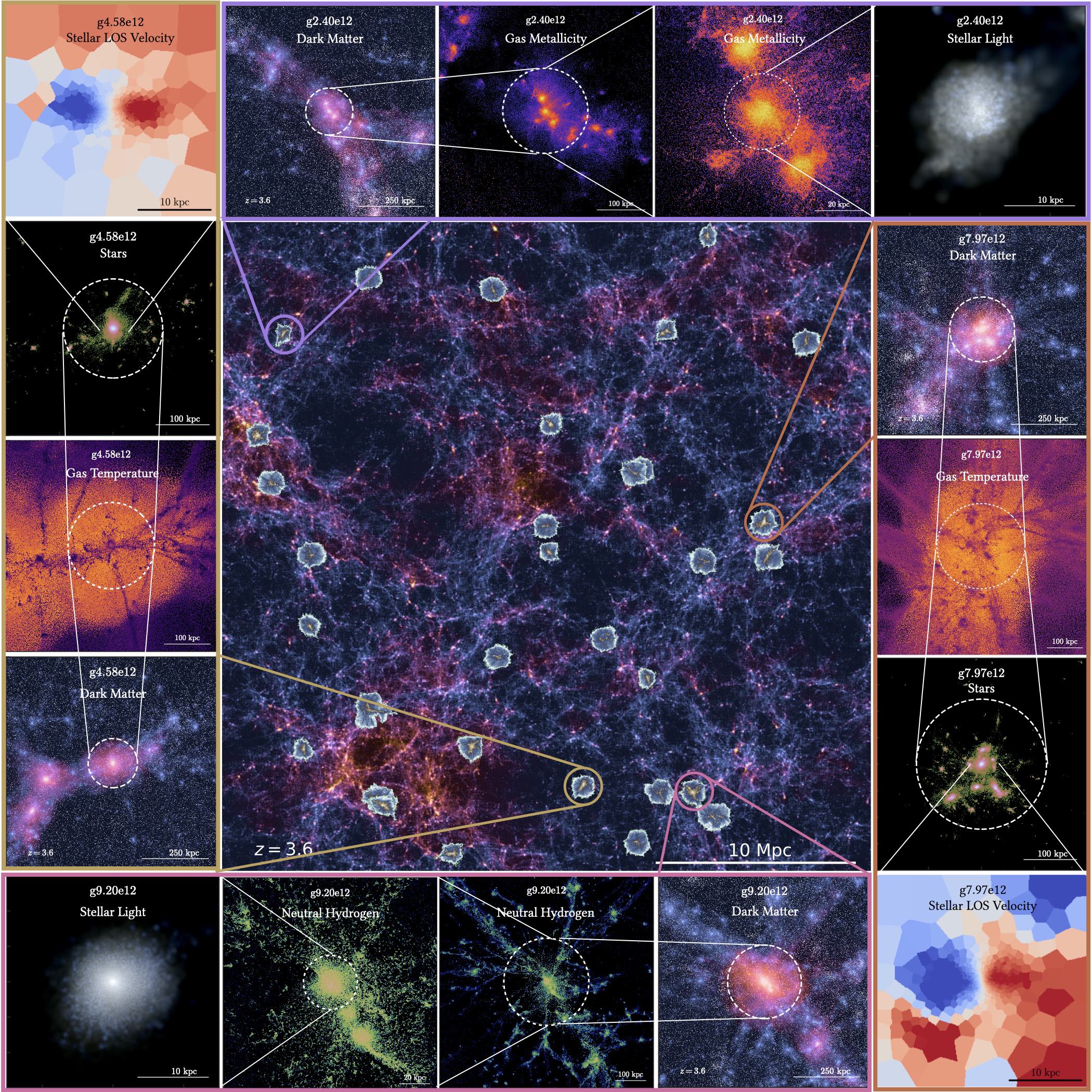
Figure 1: Highlights of the physical and numerical complexity of the "High-$z$ Evolution of Large and Luminous Objects" (HELLO) project. The central panel shows a rendering of the dark matter distribution with the 32 zoom regions overlaid on top. Four representative zoom regions are circled and the smaller panels surrounding the central panel show continuous zooms onto the central galaxy, imaging various physical quantities of the simulations, thereby highlighting the large dynamical range and physical complexity of the simulation suite.

2 Simulations

HELLO is a set of cosmological zoom-in hydrodynamical simulations at $z\sim[2,4]$ and builds on NIHAO by using the same methods for generating initial conditions, star formation and stellar feedback, and black hole growth and feedback. New implementations concern chemical element tracking and introduction of local photoionisation feedback (LPF). For completeness, we summarise every part in the coming subsections. The cosmological model employed is based on a flat $\Lambda$CDM framework, drawing on parameters from Planck Collaboration et al. (2014), and using a Hubble constant ($H_{0}$) of 67.1 $\,\mathrm{k}m\,s^{-1}\,{{{\mathrm{M}pc}}}^{-1}$. The densities associated with matter, dark energy, radiation, and baryons are given by {$\Omega_{\mathrm{m}}$, $\Omega_{\Lambda}$, $\Omega_{\mathrm{r}}$, $\Omega_{\mathrm{b}}$} = {0.3175, 0.6824, 0.00008, 0.0490}. Additionally, the power spectrum’s normalisation is set to $\sigma_{8}$ = 0.8344 and its slope to $n$ = 0.9624.

The HELLO project presently consists of two sets of 17 and 15 galaxies whose halos contain about $N_{\mathrm{part}}\sim 10^{6}$ particles within their virial radii at the final redshifts of 2.0 (age $\sim$ 3.3 Gyr) and 3.6 (age $\sim$ 1.7 Gyr), respectively (see Fig. 1 for a visual overview of the simulation volume). For the rest of this work, these two sets will be denominated ‘HELLOz2.0’ and ‘HELLOz3.6.’ Halos in HELLO are identified using the Amiga Halo Finder (AHF; Gill et al., 2004; Knollmann & Knebe, 2009). The virial radius is defined as the radius within which the halo contains an average density 200 times the critical density $\rho_{\mathrm{c}}(z)$ at redshift $z$ and is denoted as $R_{200}$.

The total mass enclosed in a sphere of radius $R_{200}$ is thus expressed as $M_{200}$ and both are related by:

$${{M_{200}}}=\frac{4}{3}\,\pi\,{{R_{200}}}^{3}\,200\,\rho_{\mathrm{c}}.$$ (1)

In the remainder of the paper, we use $M_{200}$ and $M_{\mathrm{h}alo}$ interchangeably. The simulations’ final halo masses range from $\sim$(1 to $9)\,\times 10^{12}\,{\mathrm{M}}_{\astrosun}$. HELLO thus aims at studying massive MW-like galaxies around cosmic noon (Madau & Dickinson, 2014).

Each halo is evolved hydrodynamically with the GASOLINE2 code (Wadsley et al., 2017), while a dark matter only (DMO) counterpart is run with PKDGRAV2 (Stadel, 2001, 2013). Dark matter mass and gas mass resolution in the hydro versions amount to $3.4\times 10^{6}$ ${\mathrm{M}}_{\astrosun}$ and $2.1\times 10^{5}$ ${\mathrm{M}}_{\astrosun}$, respectively, with corresponding physical softening lengths of $\epsilon_{\mathrm{DM}}=193$ (127) pc and $\epsilon_{\mathrm{gas}}=83$ (54) pc at $z=2$ (3.6). Some of the principal quantities in our simulations are summarised in Table 1. For an exhaustive list of all our simulation parameters at their respective final redshifts, see Appendix A.

Name	$z_{\mathrm{final}}$	$M_{\mathrm{halo}}$ [$10^{12}$ ${\mathrm{M}}_{\astrosun}$]	$M_{\mathrm{gas}}$ [$10^{10}$ ${\mathrm{M}}_{\astrosun}$]	$M_{\star}$ [$10^{10}$ ${\mathrm{M}}_{\astrosun}$]	$R_{200}$ [kpc]	$N_{\mathrm{part}}$
g3.08e12	2.0	2.84	7.31	10.1	142	1,943,368
g3.09e12	2.0	2.94	7.26	11.3	144	2,058,093
g3.00e12	2.0	2.43	8.33	5.91	135	1,501,948
g3.20e12	2.0	2.72	9.27	5.69	140	1,693,806
g2.75e12	2.0	2.45	8.77	9.74	135	1,778,286
g3.03e12	2.0	1.67	5.69	7.55	119	1,250,411
g3.01e12	2.0	2.67	7.41	7.67	139	1,729,071
g2.29e12	2.0	1.81	7.71	7.53	122	1,333,337
g3.35e12	2.0	1.72	6.69	2.37	120	964,316
g3.31e12	2.0	2.32	8.21	5.27	133	1,449,371
g3.25e12	2.0	2.65	8.11	4.09	139	1,643,064
g3.38e12	2.0	3.08	9.86	8.09	146	2,014,002
g3.36e12	2.0	2.08	4.43	3.14	128	1,209,250
g2.83e12	2.0	2.32	5.75	6.57	133	1,551,228
g2.63e12	2.0	2.35	7.85	9.01	133	1,682,819
g3.04e12	2.0	3.01	8.10	9.50	145	1,997,107
g2.91e12	2.0	2.11	4.33	7.29	129	1,445,948
g2.47e12	3.6	2.21	8.16	3.39	87	1,259,900
g2.40e12	3.6	2.29	5.16	0.62	88	1,231,536
g2.69e12	3.6	2.54	11.00	4.53	91	1,493,797
g3.76e12	3.6	2.58	12.30	3.45	102	1,998,769
g4.58e12	3.6	2.60	11.20	5.86	92	1,616,009
g2.71e12	3.6	1.98	9.75	4.35	84	1,216,000
g2.49e12	3.6	2.55	9.72	2.99	91	1,427,551
g2.51e12	3.6	2.52	6.57	2.61	91	1,529,843
g2.32e12	3.6	1.91	8.47	4.93	83	1,218,031
g2.96e12	3.6	2.84	12.70	3.43	95	1,605,548
g7.37e12	3.6	5.76	20.70	11.60	120	3,526,490
g7.97e12	3.6	5.89	13.80	7.12	121	3,546,175
g9.20e12	3.6	8.74	25.70	14.10	138	5,318,120

Table 1: Final HELLO sample at $z=2.0$ and $z=3.6$ used in this paper. The columns are: galaxy name (a reference to the low-resolution halo mass at the final redshift); final redshift ($z_{\mathrm{final}}$); halo ($M_{\mathrm{halo}}$), gas ($M_{\mathrm{gas}}$), and stellar ($M_{\star}$) masses within 20 per cent of the virial radius ($R_{200}$); and total number of particles in the halo ($N_{\mathrm{part}}$).

Unless otherwise specified, galactic quantities such as, e.g., ${{M_{\star}}}$, gas mass ($M_{\mathrm{gas}}$), ${{R_{\mathrm{e}}}}$, and SFR are computed using the corresponding particles within 20 per cent of $R_{200}$ to remain consistent with NIHAO simulations. While small satellites may be present at these distances, we control the resulting stellar mass, effective radius, effective stellar surface density, and SFR so they do not vary by more than $\sim$10 per cent with respect to using $0.1\,{{R_{200}}}$. The two galaxies that didn’t pass these criteria were removed from the remaining calculations. A more detailed discussion can be found in Appendix B.

We show in Fig. 2, a visual aperçu of six HELLO galaxies, three belonging to the HELLOz2.0 sample (top three rows) and three to the HELLOz3.6 sample (bottom three rows). The first three columns from left to right are a face-on view of dark matter, stars, and H i gas, respectively. The last two columns show an image rendering in face- and edge-on views of stars in the wavelength bands $I$, $V$, and $U$. The white dashed circle represents the virial radius, and the simulation name, as well as a distance scale is displayed in each panel. Our simulations exhibit a variety of morphologies, from relatively thin disks to more compact and spherical objects, as well as different local environments with some galaxies like g2.75e12, g3.03e12, and g4.58e12 fairly isolated, while g2.83e12 and g9.20e12 are about to merge with surrounding satellites.

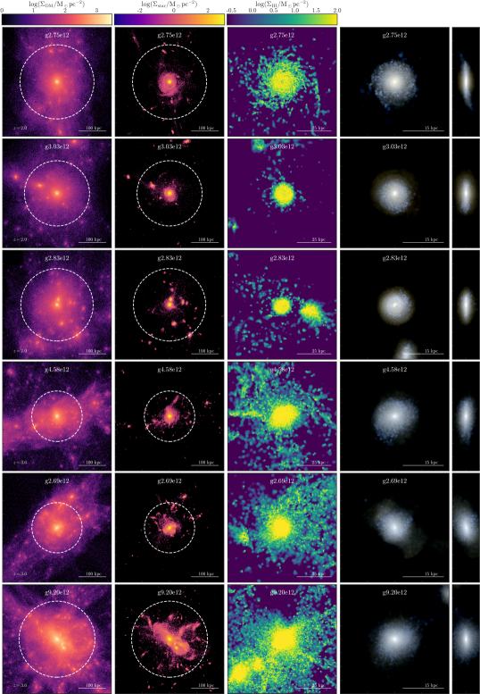
Figure 2: Surface density maps viewed face-on as well as stellar face- and edge-on images in the wavelength bands $I$, $V$, and $U$ for six example galaxies (three at $z=2$ and three at $z=3.6$). The surface density columns from left to right are: dark matter, stars, and H i gas. The white dashed circle indicates the virial radius (${{R_{200}}}$).

2.1 Initial conditions

All halos are picked from a cosmological DMO volume simulation of size $100\,{h^{-1}\mathrm{M}pc}^{3}$ at $z=0$ and containing $400^{3}$ particles with constant mass resolution, created with PKDGRAV2. The motivation for these particular values is to allow for a sufficient number of virialised halos of masses $M_{\mathrm{halo}}\sim 10^{12}$ ${\mathrm{M}}_{\astrosun}$ at the target redshifts, which can then be ‘zoomed-in’ and evolved hydrodynamically. The halos are selected to be isolated, i.e., there are no other structures within $2\,{{R_{200}}}$. The zoom-in initial conditions are generated using an adapted version of the GRAFIC2 software (Bertschinger, 2001).

The refinement level is set such as to keep a constant ratio between the dark matter (DM) force softening ($\epsilon_{\mathrm{DM}}$) and $R_{200}$, resolving the DM mass profile down to $\mathrel{\hbox{\hbox to0.0pt{\hbox{\lower 4.0pt\hbox{$\sim$}}\hss}\hbox{$<$}}}$$0.01\,{{R_{200}}}$. We adopt here a DM softening length of 1/80 the inter-particle distance in the highest resolution region and the gas gravitational softening is calculated following $\epsilon_{\mathrm{gas}}=\epsilon_{\mathrm{DM}}\,\sqrt{\Omega_{\mathrm{b}}/\Omega_{\mathrm{DM}}}$, where $\Omega_{\mathrm{DM}}=\Omega_{\mathrm{m}}-\Omega_{\mathrm{b}}$. The choice of 1/80 is motivated by the fact that it still satisfies the lower threshold set by the virial radius and the number of particles within $R_{200}$ of $\epsilon>{{R_{200}}}/\sqrt{N_{200}}$, as suggested by Power et al. (2003), while better resolving the dynamical interactions than NIHAO (where the softening fraction is 1/40). Moreover, recent work (Zhang et al., 2019) showed that softening fractions of 1/80 and 1/100 converge to smaller radii as compared to the optimal softening length proposed by Power et al. (2003).

2.2 Star formation and stellar feedback

The formation of stars follows the Kennicutt-Schmidt law (Schmidt, 1959; Kennicutt, 1998) and is implemented as described in Stinson et al. (2006, 2013). First, to be eligible to form stars, gas particles have to satisfy both a temperature ($T<15000$ K) and density ($n>10$ cm^-3) threshold. The theoretical maximum gas density that we are able to resolve is $n_{\mathrm{max}}\sim 80$ cm^-3, according to:

$$n_{\mathrm{max}}\approx N_{\mathrm{smooth}}\,\frac{m_{\mathrm{gas}}}{\epsilon_{\mathrm{gas}}^{3}},$$ (2)

where $N_{\mathrm{smooth}}=50$ is the number of neighbouring particles within the smoothing kernel and $m_{\mathrm{gas}}$ is the gas particle initial mass. In practice, however, gas can reach higher densities with a maximum value determined by the minimal smoothing length, $h_{\mathrm{min}}=0.25\,\epsilon_{\mathrm{gas}}$. In spite of halving the softening factor, we maintain the NIHAO threshold density of 10 cm^-3, since higher thresholds have been shown to underproduce stars relative to abundance matching at $z=0$ for halos with ${{M_{200}}}>10^{11}\,{\mathrm{M}}_{\astrosun}$ (Dutton et al., 2020). Gas particles satisfying the aforementioned criteria are allowed to convert to stars following:

$$\frac{\Delta M_{\star}}{\Delta t}=c_{\star}\,\frac{M_{\mathrm{gas}}}{t_{\mathrm{dyn}}},$$ (3)

where the mass of stars ($\Delta M_{\star}$) formed between each timestep ($\Delta t$) is a fraction $c_{\star}=0.1$ of the theoretical SFR expressed as the eligible gas mass ($M_{\mathrm{gas}}$) that could form stars during one dynamical time ($t_{\mathrm{dyn}}$).

Stellar feedback is modeled in three different ways, depending on the epoch and stellar mass. First, feedback energy from young bright stars is released in their vicinity during the first 4 Myr after a star particle is born and is denoted as early stellar feedback (ESF). The method adopts the model from Stinson et al. (2013) and is implemented as a fraction $\epsilon_{\mathrm{ESF}}=0.13$ of the stellar luminosity being ejected as isotropic thermal energy into the surrounding gas. The energy released by these stars typically represents $2\times 10^{50}$ erg ${\mathrm{M}}_{\astrosun}^{-1}$ over the first 4 Myr after the creation of the stellar particle, and gas radiative cooling is left on during this epoch.

After the initial phase, supernovae (SNe) are initiated for stars with initial masses between 8 and 40 ${\mathrm{M}}_{\astrosun}$ within the stellar population. The actual number of SNe is calculated from the stellar initial mass function (IMF), energy, mass, and metals ejected around the regions where the stars formed. In practice, the energy released is $10^{51}$ erg per SN and feedback from SNe is modeled according to the blast wave formalism described in Stinson et al. (2006). Affected gas particles see their radiative cooling turned off. Finally, stars forming with masses below 8 ${\mathrm{M}}_{\astrosun}$ constantly eject mass and metals as stellar winds. At each timestep, the mass range of stars that are supposed to die is computed and the corresponding returned mass fraction is determined (Stinson et al., 2006).

2.3 Chemistry

Star particles in cosmological simulations do not resolve individual stars, but are tracer particles representing a population of stars, referred to as a simple stellar population (SSP), that is described by a single age ($\tau_{\mathrm{star}}$), a metallicity ($Z_{\mathrm{star}}$), and an IMF specifying the number of stars in a given mass bin. In our simulations, we chose a Chabrier (2003) IMF. We do not adopt a particular stellar evolution model, instead use the chemical evolution code Chempy (Rybizki et al., 2017) in order to synthesise the final stellar evolution model and the corresponding yield tables to be used for each run. Hence, Chempy calculates the time evolution of the chemical yields for an SSP. The stellar nucleosynthetic yields include the relative mass return fractions from three channels: type Ia supernova (SN Ia), core-collapse supernova (SN II), and asymptotic giant branch (AGB) stars.

Elemental feedback from these three channels is implemented as described in Buck et al. (2021). We tabulate the time-resolved, mass-dependent element release of a single stellar population as a function of initial metallicity in a grid of 50 metallicity bins, logarithmically-spaced between $10^{-5}$–0.05 in metallicity. Each metal bin is resolved by 100 time bins, logarithmically-spaced in time and ranging from 0 to 13.8 Gyr (the age of the Universe in our adopted cosmographic parameters). Our fiducial combination of yield tables uses SN Ia yields from Seitenzahl et al. (2013), SN II yields from Chieffi & Limongi (2004), and AGB star yields from Karakas & Lugaro (2016). All our simulations track the evolution of the 10 most abundant elements by default (H, He, O, C, Ne, Fe, N, Si, Mg, and S) while any other element present in the yield tables can additionally be tracked. For HELLO galaxies, we also track the six following elements: Na, Al, Ca, Ti, Sc, and V.

2.4 Local photoionisation feedback

High-energy ionisation photons from extragalactic sources are an important part of galaxy formation models and can provide a negative feedback affecting gas inflow and cooling (Haardt & Madau, 1996). While such external ultraviolet background (UVB) radiation can be approximated as isotropic on large cosmological scales, the local high-energy photon sources (stars, hot gas, or BHs) within the galaxy are distributed highly anisotropically. Photoionisation and photoheating from three types of local radiation sources is implemented on top of the Faucher-Giguère et al. (2009) UVB in an optically-thin approximation, as described in Obreja et al. (2019). The three source types are: young stars ($\tau_{\mathrm{star}}<10$ Myr), post-AGB stars ($\tau_{\mathrm{star}}>200$ Myr), and bremsstrahlung from hot gas in three temperature bins: $5.5<\log(T/\mathrm{K})<6.5$, $6.5<\log(T/\mathrm{K})<7.5$, and $7.5<\log(T/\mathrm{K})<8.5$.

We directly use the Cloudy (Ferland et al., 1998) photoionisation models with the combinations of sources computed by Kannan et al. (2016). As young stars can still be partially enshrouded in their parent molecular clouds, only a fixed 5 per cent of emitted photons are assumed to escape the local environment (Kannan et al., 2014). The other types of sources are assumed to have an escape fraction $f_{\mathrm{esc}}=1$. Dense gas shielding from the local radiation field is modeled by a simple density-dependent relation, in which all gas particles with densities $n>0.1$ cm^-3 receive an exponentially attenuated local radiation field. We prefer an attenuated field over an abrupt cutoff in order to emulate a smoother transition between shielded and partially-shielded regions.

2.5 Black hole growth and feedback

In HELLO, the implementation of black hole (BH) and AGN feedback is performed according to Blank et al. (2019). Whenever the mass of a halo surpasses the threshold of $5\times 10^{10}\,{\mathrm{M}}_{\astrosun}$, the gas particle with the lowest gravitational potential is converted into a seed BH of initial mass $M_{\mathrm{seed}}=10^{5}\,{\mathrm{M}}_{\astrosun}$. The BH particle is then allowed to accrete and release feedback energy according to Springel et al. (2005). The mass accretion is governed by Bondi accretion (Bondi, 1952), scaled by a boost parameter, $\alpha=70$:

$$\dot{M}_{\mathrm{Bondi}}=\alpha\,\frac{4\pi\,G^{2}\,M_{\bullet}^{2}\,\rho_{\mathrm{gas}}}{(c_{\mathrm{s}}^{2}+v_{\mathrm{gas}}^{2})^{3/2}},$$ (4)

with the BH mass $M_{\bullet}$, and $\rho_{\mathrm{gas}}$, $c_{\mathrm{s}}$, and $v_{\mathrm{gas}}$, the surrounding gas density, sound speed, and velocity, respectively. The $\alpha$ parameter accounts for the finite resolution in simulations and its value is the optimal value found by Blank et al. (2019).

The Eddington accretion rate (Eddington, 1921):

$$\dot{M}_{\mathrm{Edd}}=\frac{M_{\bullet}}{\epsilon_{\mathrm{r}}\,\tau_{\mathrm{S}}}$$ (5)

defines an upper bound for the accretion, as it is the rate at which the gravitational infall of gas is counter-balanced by the radiative pressure. In Equation 5, the Salpeter timescale ($\tau_{\mathrm{S}}$, Salpeter, 1964) and the radiative efficiency ($\epsilon_{\mathrm{r}}$) are set to 450 Myr and 0.1, respectively.

During each timestep ($\Delta t$), the mass ($\dot{M}_{\bullet}\,\Delta t$) is accreted from the most gravitationally-bound gas particle, with $\dot{M}_{\bullet}\equiv\min\,\{\dot{M}_{\mathrm{Bondi}},\,\dot{M}_{\mathrm{Edd}}\}$. If the gas particle’s mass is less than 20 per cent of its initial mass, the particle is removed from the simulation and its mass and momentum are distributed and weighted among the neighbours within the smoothing kernel. The increase of $\Delta M_{\bullet}$ in BH mass is accompanied by an increase of its softening length to avoid too small steps due to large accelerations. Finally, the thermal energy feedback resulting from accretion can be expressed as a fraction $\epsilon_{\mathrm{f}}=0.05$ of the BH luminosity $L$:

$$\dot{E}=\epsilon_{\mathrm{f}}\,\dot{L}=\epsilon_{\mathrm{f}}\,\epsilon_{\mathrm{r}}\,\dot{M}_{\bullet}\,c^{2}.$$ (6)

The thermal energy is distributed among the 50 nearest gas particles around the BH, weighted by the kernel function.

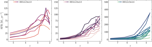
Figure 3: Individual SFHs of our simulations. From left to right: HELLOz2.0 galaxies whose SFRs are declining towards their final redshift, HELLOz2.0 galaxies whose SFRs are still rising, and HELLOz3.6. The colour gradient maps the final stellar mass from lighter (lower mass) to darker (higher mass) shades.

3 Star-formation rate and history

Our simulations confirm the higher SFRs observed in the early Universe. At $z=2$, SFRs within the HELLO galaxies span from 35 ${\mathrm{M}}_{\astrosun}$ yr^-1 to 102 ${\mathrm{M}}_{\astrosun}$ yr^-1, with an average of 67 ${\mathrm{M}}_{\astrosun}$ yr^-1. Earlier at $z=3.6$, the galaxies in our sample exhibit more star-forming activity, which translates to an increased average SFR of 152 ${\mathrm{M}}_{\astrosun}$ yr^-1, but also broader variations, with rates extending from 21 ${\mathrm{M}}_{\astrosun}$ yr^-1 to 355 ${\mathrm{M}}_{\astrosun}$ yr^-1. These values are computed by summing up the formation mass of all stars located within $0.2\,{{R_{200}}}$ in the last 100 Myr and averaging over the same timescale. Our goal is to ensure the most appropriate comparison to observations as possible, since observations usually infer SFRs from a combination of infrared and ultraviolet luminosities, which are believed to trace the SFR of galaxies over the last 100 Myr (see, e.g., Speagle et al., 2014; Madau & Dickinson, 2014; Förster Schreiber & Wuyts, 2020). On top of our fiducial SFR, we also compute a more instantaneous SFR averaged over 10 Myr, which we do not use in this paper, but include in Table 3, for completeness.

In Fig. 3, we plot the star formation history (SFH) of each galaxy in both our samples. The colour gradients are sorted from light to dark by increasing stellar mass at the final redshift. While all HELLOz3.6 galaxies exhibit rising SFRs up to their final redshift (right panel), the variety of SFH shapes is richer in the HELLOz2.0 sample. Indeed, some galaxies display an overall continuously-rising SFR (middle panel), but others seem to have reached their peak SFR and are on the decline (right panel). A galaxy’s SFR is considered to be declining if the SFR at $z=2$ is lower than in the last two snapshots. Moreover, for the rest of this paper, we will assume that the galaxies with declining SFRs have begun their journey towards becoming quiescent, and we denote them as ‘post-peak,’ as opposed to those that have not yet reached their peak SFR, designated as ‘pre-peak.’

We combine all SFHs in a single plot in Fig. 4 by showing the median of each sample as thick curves (HELLOz2.0 pre- and post-peak: orange and purple; HELLOz3.6: turquoise), and the region encompassing the 16th to 84th percentiles as a shaded area. Fig. 4 gives a clear picture of the different regimes in which our simulations find themselves. HELLOz3.6 galaxies are significantly more efficient at forming stars than their HELLOz2.0 counterparts, which comes at no surprise given that they reach similar end masses in roughly half the time. On the other hand, both pre- and post-peak simulations feature a slower evolution until both samples reach a median SFR of $65\,{\mathrm{M}}_{\astrosun}\,\mathrm{yr}^{-1}$. Post-peak galaxies, however, consistently have a higher median SFR, peaking at $93\,{\mathrm{M}}_{\astrosun}\,\mathrm{yr}^{-1}$ around $z=2.3$. Importantly, the final stellar masses in the pre-peak sample range from $2.4\times 10^{10}$ to $9.0\times 10^{10}\,{\mathrm{M}}_{\astrosun}$, somewhat below the post-peak sample ranging from $7.3\times 10^{10}$ to $1.1\times 10^{11}\,{\mathrm{M}}_{\astrosun}$. That is, post-peak galaxies are slightly more massive and thus, might be ‘further’ in their evolution.

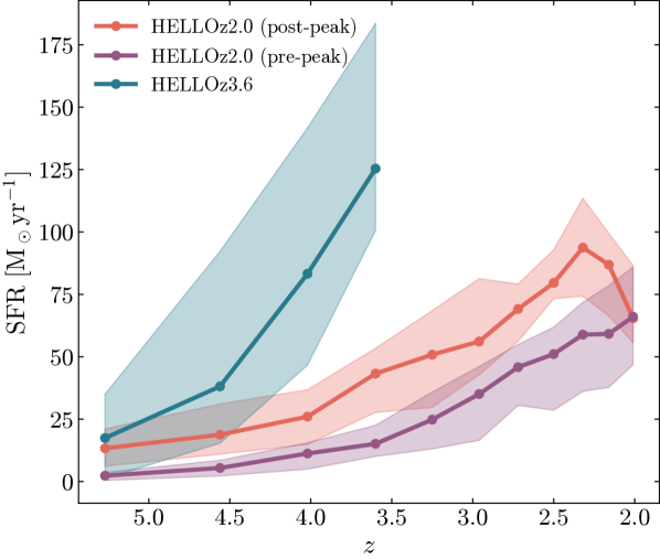
Figure 4: Median SFHs of HELLOz2.0 post-peak (orange), pre-peak (purple), and HELLOz3.6 (turquoise) galaxies. The medians are calculated at each redshift from the curves in Fig. 3. The shaded areas encompass the 16th and 84th percentiles.

4 Scaling relations

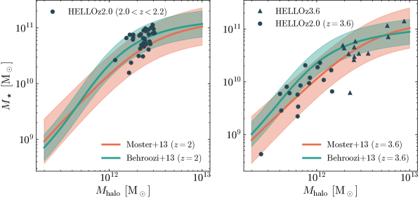
Figure 5: Stellar-to-halo mass relation for HELLO galaxies compared to abundance matching expectations from Moster et al. (2013) (orange curve) and Behroozi et al. (2013) (green curve) at $z=2$ (left panel) and $z=3.6$ (right panel). The shaded area represents the $\pm 1\,\sigma$ scatter around the respective relations. In the left, we show HELLOz2.0 snapshots between redshifts 2.0 and 2.2, while on the right we show HELLOz3.6 final snapshots, as well as HELLOz2.0 progenitors at $z=3.6$.

4.1 Stellar-to-halo mass relation

We plot the stellar-to-halo mass relation (SHMR) of HELLO galaxies in Fig. 5 and compare it against expectations from abundance matching (Moster et al., 2013; Behroozi et al., 2013) at $z=2$ (left panel) and $z=3.6$ (right panel). The shaded regions show the $\pm 1\,\sigma$ scatter around the respective relations. Black dots represent HELLOz2.0 galaxies between redshifts $2.0<z<2.2$ (left) and at $z=3.6$ (right). Triangles in the right panel are the final snapshots of the HELLOz3.6 sample, while circles are HELLOz2.0 progenitors at $z=3.6$.

Our simulations agree well with both relations, as expected, since NIHAO galaxies have already been shown to match the ${{M_{\star}}}$–${{M_{200}}}$ relation well up to $z=4$ (Wang et al., 2015; Blank et al., 2019), translating to an appropriate calibration of star formation density threshold and feedback efficiencies. We experimented with a higher $n=80$ cm^-3, but the resulting galaxies underproduced stars at $z=0$, an issue already covered in §2.2. Using such a value would require a lengthy recalibration of the feedback efficiencies, which we might do in the future. For this work, although we found no significant discrepancies between fiducial galaxies run with $n=10$ cm^-3 and $n=80$ cm^-3 at high redshift, we required the SHMR to be in agreement at $z=0$.

4.2 The main sequence of star formation

We begin by plotting the SFR–$M_{\star}$ relation for our galaxies in Fig. 6. The figure contains all snapshots of all galaxies from both HELLOz2.0 (circles) and HELLOz3.6 (triangles) samples, colour-coded in redshift bins from $z=7$ down to $z=2$. Each point represents the SFR from stars that formed in the last 100 Myr of each snapshot, plotted against the respective stellar mass of each galaxy. We find that HELLO galaxies are relatively tightly correlated across the entire sample.

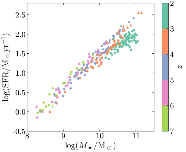
Figure 6: Stellar mass versus SFR of all our simulation snapshots, colour-coded in redshift bins from $z=2$ to $z=7$. Galaxies belonging to the HELLOz2.0 sample are marked as circles, while those belonging to HELLOz3.6 are marked as triangles.

The general consensus among observations is that the scatter around the main sequence is roughly constant at 0.2–0.3 dex across the entire mass range, as well as redshifts probed (Speagle et al., 2014), and simulations do agree overall with this picture (e.g., Kannan et al., 2014; Torrey et al., 2014; Sparre et al., 2015). Qualitatively, Fig. 6 exhibits low scatter at all masses and in each redshift bin, as well. As previously mentioned, unanimity regarding the existence of a turnover mass and flattening of the star-forming main sequence (SFMS) has yet to be found. However, when apparent, it is encountered at lower redshifts and tends to vanish above $z\sim 2$.

HELLO galaxies exhibit a similar behaviour, where the relation between $z=3$–5 (orange and blue points) does not show any sign of a shallower slope. The same cannot be said for the turquoise points in redshift bin 2–3 that seem to flatten above $\log(M_{\star}/{\mathrm{M}}_{\astrosun})\sim 10.5$. Finally, for each redshift bin containing the progenitors of the galaxies in the next one (from green to turquoise), our plot shows that HELLO simulations evolve smoothly along the SFMS across cosmic times. Interestingly, this coevolution between HELLOz3.6 and HELLOz2.0 seems to break around $\log(M_{\star}/{\mathrm{M}}_{\astrosun})\sim 10$, above which HELLOz2.0 galaxies show signs of weakening star formation growth.

We compare the SFR–$M_{\star}$ relation of our galaxies with various observations in Fig. 7. Unlike the last figure, only the three (two) final snapshots of HELLOz2.0 (HELLOz3.6) are shown in the top and bottom panels, respectively. The concerned redshift ranges are $2.0<z<2.3$ and $3.6<z<4.0$, as indicated in the legends. In addition, HELLOz2.0 snapshots at $3.6<z<4.0$ are added to the lower panel. The shape of the points follows the same convention as before, i.e., galaxies from HELLOz2.0 are represented as circles and the ones from HELLOz3.6 as triangles.

In the upper panel, our simulations are compared to the empirical SFR–$M_{\star}$ relations identified by Schreiber et al. (2015) (red), Tomczak et al. (2016) (green; continuous line for all galaxies and dotted for star-forming galaxies only), Barro et al. (2017) (purple), and Pearson et al. (2018) (yellow). All these relations together cover redshifts spanning from $z=1.8$ to $z=2.3$. We furthermore display the quiescent cutoff from Barro et al., defined as 0.7 dex below their SFMS, shown here with a dashed grey line. In the lower panel, the colours follow the same convention, with the addition of a second redshift bin from Pearson et al. (dark purple). Together, these observed relations cover redshifts ranging from $z=2.9$ to $z=4.9$.

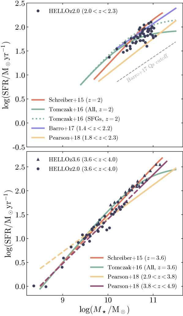
Figure 7: Stellar mass versus SFR for HELLOz2.0 between redshifts of 2.0 and 2.3 (top; circles) and HELLOz3.6 between redshifts of 3.6 and 4.0 (bottom; triangles) compared to various relations found in the literature, indicated in the legend. In the bottom panel, we add HELLOz2.0 progenitors in the same redshift range (circles). For the observed relations, a dashed line indicates an extrapolation to lower masses.

The upper panel of Fig. 7 exhibits good agreement with observations. Specifically, our simulations nicely embrace the curve from Tomczak et al. (all galaxies) and seem consistent with a turnover and flattening. The lack of galaxies covering a wider range in stellar mass around $z\sim 2$, however, prevents us from making stronger claims. HELLOz2.0 slightly undershoots Schreiber et al. and Barro et al., as well as the sample restricted to star-forming galaxies (SFGs) from Tomczak et al. This could indicate that some of our galaxies might have begun their quenching phase, which we will address in Section 5. Nevertheless, all our galaxies are well above the quiescent cutoff from Barro et al. and are therefore all considered to be still star-forming, having SFRs well in the order $10\,{\mathrm{M}}_{\astrosun}\,\mathrm{yr}^{-1}$. Finally, our galaxies visually recover the slope from Pearson et al., but systematically overpredict the normalisation.

Moving on to the lower panel of Fig. 7, HELLO galaxies in the redshift range $3.6<z<4.0$ reproduce the observed SFMS extremely well across the two orders of magnitude of masses probed. The only exception is Pearson et al. for redshifts $2.9<z<3.8$, whose slope is shallower than the two other predictions, as well as their higher redshift bin sample. At these early cosmic times, the turnover is expected to be virtually non-existent, although Tomczak et al. found a significant flattening still occurring at about $M_{\star}\sim 10^{11}$ ${\mathrm{M}}_{\astrosun}$. Unfortunately, our sample does not contain a sufficient number of galaxies with high enough stellar masses to make any assessment to the question.

4.3 Size versus mass relation

Fig 8 shows the size-mass relation of HELLOz2.0 ($2.0<z<2.3$) galaxies plotted against the observed relation at $z=2.25$ inferred by van der Wel et al. (2014). We split our simulated galaxies into pre-peak (black dots) and post-peak (black stars) samples. The blue and red lines are the observed relations for star-forming and quiescent galaxies, respectively, and the shaded regions demarcate the $1\sigma$ scatter bounds. In their work, van der Wel et al. studied the evolution of the size-mass distribution over the redshift range $0<z<3$, using data from the 3D-HST (Brammer et al., 2012) and CANDELS (Grogin et al., 2011) surveys. While in broad agreement with the relations from SFGs, HELLOz2.0 pre-peak galaxies tend to underpredict the relation and this trend is accentuated with increasing stellar mass. Moreover, post-peak galaxies are systematically outside the $1\sigma$ region and lie in between the relation from star-forming and quiescent galaxies. We propose several explanations for the trend seen in Fig. 8 that could explain why HELLO galaxies are somewhat smaller than expected from observations.

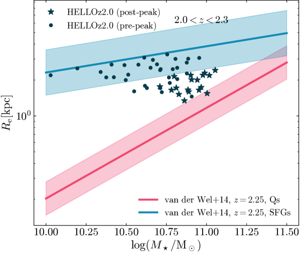
Figure 8: Size (effective radius, $R_{\mathrm{e}}$) versus (stellar) mass relation of HELLOz2.0 simulations between redshifts of 2.0 and 2.3, compared to the observed relations determined by van der Wel et al. (2014) for quiescent (red) and star-forming (blue) galaxies. The respective shaded regions depict the $\pm 1\,\sigma$ scatter bounds. HELLOz2.0 post-peak galaxies and their progenitors are marked as stars. Similarly, pre-peak galaxies are depicted as circles.

First, Arora et al. (2023) compared a multitude of scaling relations between NIHAO simulations and local galaxies from the MaNGA survey (Bundy et al., 2015; Wake et al., 2017) and found the high-mass simulations above ${\log(M_{\star}/\mathrm{M}_{\odot})}\sim 10$ tend to lie below the locus of the observed size-mass relation. A possible cause could be a relative weakening of the stellar feedback with respect to the galaxy mass, which in turn prevents over-cooling and baryonic accretion towards the center of a galaxy (see, e.g., McCarthy et al., 2012). This effect can potentially be balanced by a take over from AGN feedback, but the latter might not be strong enough yet (see Section 5). With NIHAO and HELLO sharing the same hydrodynamical code, we argue that similar effects could be at play in our case.

Second, we do not apply any magnitude cutoff in the calculation of the effective radius. We use the pynbody.analysis.luminosity.half_light_r() method from PYNBODY (Pontzen et al., 2013), applied to all stars within 20 per cent of the virial radius. This method calculates the radius at which half of the total luminosity in the given band (here $V$) is reached. Furthermore, Ma et al. (2018) have shown that the observed size of a galaxy can significantly depend on the surface brightness limit of a given observation campaign. Taken at face value, this limiting factor tends however to an underestimation of $R_{\mathrm{e}}$ rather than the opposite. Finally, the fact that our post-peak galaxies are the furthest from the SFG size-mass relation (and the closest to the quenched relation) is another piece of evidence suggesting that these galaxies have indeed started their quenching phase. This will be further addressed in the next subsection after investigating the size evolution track across time in our simulations.

4.4 Size evolution

While in Fig. 8 we looked at the distribution of galaxies in the size-mass relation at a fixed redshift, we now investigate how the median sizes of our different samples evolve with time. Fig. 9 displays the median effective radius as a function of redshift since $z=8$ for HELLOz2.0 (all galaxies; black), HELLOz2.0 pre- and post-peak (purple and orange dashed lines), and HELLOz3.6 (all galaxies; turquoise). For comparison, the size evolution recently observed by Ormerod et al. (2024) from galaxies within the CEERS survey (Finkelstein et al., 2017, 2023; Bagley et al., 2023), using JWST NIRCam imaging (Rieke et al., 2023), is shown in green with the $\pm 1\,\sigma$ scatter around it.

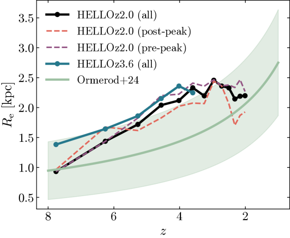
Figure 9: Median size evolution of HELLO galaxies. The black and turquoise curves represent all galaxies from HELLOz2.0 and HELLOz3.6, respectively. We further split the HELLOz2.0 sample into post-peak (orange dashed line) and pre-peak (purple dashed line). The observed relation with the $\pm 1\,\sigma$ scatter from Ormerod et al. (2024) is shown in green.

Since $z=8$, our simulations exhibit a steady increase in the median size across all samples down to $z\sim 3$. Below $z\sim 3$, our sizes flatten (or even contract) for the post-peak sample, and finish on the observed relation at $z=2$. Individually, some of our simulations undergo very large variations in $R_{\mathrm{e}}$ due to mergers, but these outliers do not significantly affect the median results. It is important to stress that Fig. 9 does not represent an ‘apples-to-apples’ comparison with Ormerod et al., because they use galaxies with $\log(M_{\star}/\mathrm{M}_{\odot})>9.5$ at all redshifts, whereas our curves follow the median evolutionary track of individual galaxies, whose masses increase with time. The HELLOz2.0 and HELLOz3.6 samples reach a median stellar mass of $\log(M_{\star}/\mathrm{M}_{\odot})=10$ at $z=3.5$ and $z=4.7$, respectively.

Comparing Figs. 4 and 9, specifically the orange curves, the steeper SFR growth from 55 to 94 ${\mathrm{M}}_{\astrosun}\,\mathrm{yr}^{-1}$ between $z=3$ and $z=2.3$ corresponds to a precipitous compaction of the median size from the peak at $R_{\mathrm{e}}=2.4$ kpc down to 1.7 kpc. During the last 400 Myr, while these galaxies’ median SFR decreases abruptly to 65 ${\mathrm{M}}_{\astrosun}\,\mathrm{yr}^{-1}$, their median size grew by 0.2 kpc to reach 1.9 kpc. This behaviour is consistent with previous results from cosmological simulations (Wellons et al., 2015; Tacchella et al., 2016). HELLOz2.0 pre-peak galaxies follow a similar, yet smoother evolution. Their median SFR growth picks up at $z=3.6$ and evolves steadily from 15 to 65 ${\mathrm{M}}_{\astrosun}\,\mathrm{yr}^{-1}$ at $z=2$.

In the meantime, their median effective radius stabilizes at 2.4 kpc and slightly decreases to 2.3 kpc by $z=2$. We attribute this more gentle size evolution to the corresponding slightly lower stellar mass and SFR. Finally, HELLOz3.6 features a comparable growth until $z=4$, reaching a median size of 2.3 kpc before contracting to 2.2 kpc in the last snapshot. While marginal, this contraction follows an analogous pattern to HELLOz2.0, occurring at similar masses (see Fig. 10 and its description below). This suggests similar evolutionary mechanisms at play.

Fig. 10 shows the size evolution of HELLO galaxies versus their stellar masses. The colours remain the same as in the previous figure and we plot for each snapshot the median value of $R_{\mathrm{e}}$ as a function of the median value of the stellar mass at the given epoch. The half-light radii of both samples evolve similarly and both show their growth saturating and contracting above ${\log(M_{\star}/\mathrm{M}_{\odot})}\sim 10$. Moreover, until the contraction of the black curve, HELLO simulations are systematically larger at lower redshift and fixed mass. Above ${\log(M_{\star}/\mathrm{M}_{\odot})}\sim 10$, the disparity tends to vanish, due to the post-peak simulations undergoing a phase of significant compaction.

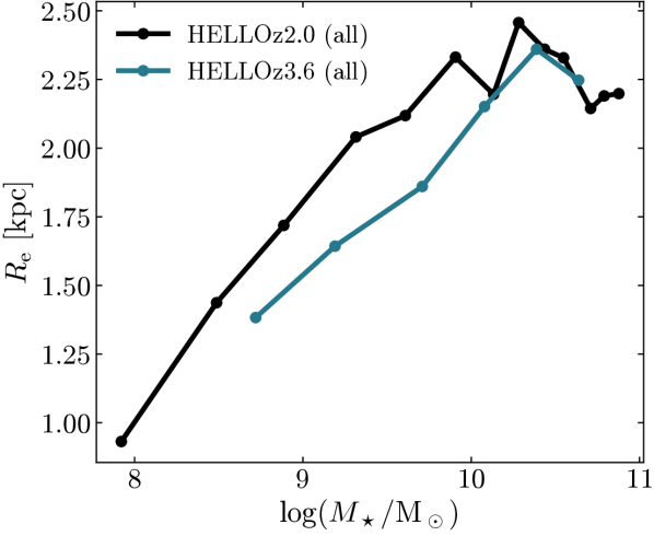
Figure 10: Median size evolution of HELLO galaxies with respect to the median stellar mass of each snapshot. The black and turquoise curves represent all galaxies from HELLOz2.0 and HELLOz3.6, respectively.

Our results also match the general picture found by other simulations. Furlong et al. (2017) analysed the size of galaxies at $0<z<2$ from the EAGLE (Schaye et al., 2015; Crain et al., 2015) suite and found that it simultaneously depends on stellar mass, redshift, as well as star formation classification. In other words, galaxy sizes are positively correlated with stellar mass and anti-correlated with redshift, and star-forming galaxies are typically larger than their quiescent counterparts at fixed stellar mass. Similar results in positive and negative correlations of galaxy size with stellar mass and cosmic time are found by Ma et al. (2018) using FIRE-2 (Hopkins et al., 2018) at $z\geq 5$. However, we want to emphasise again that at fixed stellar mass, HELLO galaxies at higher redshift are smaller only up to ${\log(M_{\star}/\mathrm{M}_{\odot})}\sim 10$, and the picture becomes more convoluted above this value.

4.5 Surface density scaling relations

We now turn our attention to the surface density scaling relations, namely the correlations between the surface mass density $\Sigma_{r}=M_{\star}(<r)/4\pi r^{2}$, and the stellar mass for a given radius $r$. In what follows, we calculate $\Sigma_{1}$ and $\Sigma_{\mathrm{e}}$, representing the densities enclosed within radii of 1 kpc and the effective radius ${{R_{\mathrm{e}}}}$, respectively. In Fig. 11, we investigate how our $z=2$ sample compares to Barro et al. (2017) in the surface density to stellar mass relation. The upper and lower panels show $\Sigma_{1}$ and $\Sigma_{\mathrm{e}}$ against $M_{\star}$, respectively. We use snapshots covering the $2<z<2.2$ range and mark galaxies belonging to the post-peak subsample as stars. The red and blue lines represent a power law fit to a selection of massive galaxies from the CANDELS GOODS-S catalogue (Guo et al., 2013) for quiescent (red) and star-forming (blue) galaxies, and the shaded regions are the $\pm 1\,\sigma$ scatter around the relations. In their paper, Barro et al. found that both relations have been in place since $z\sim 3$ with practically no change in slope or scatter ever since.

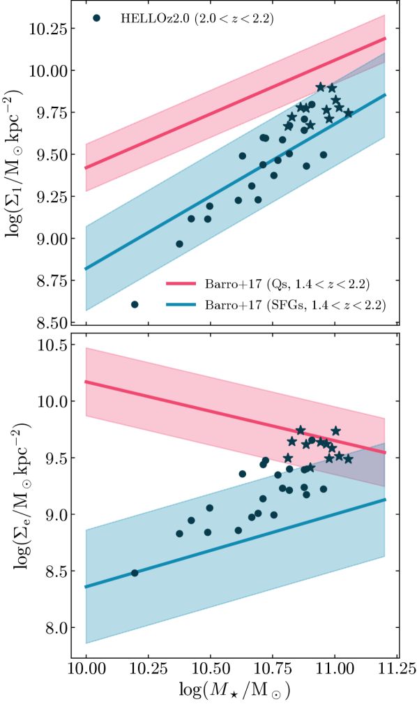
Figure 11: Surface density versus stellar mass relations of HELLOz2.0 simulations between redshifts of 2.0 and 2.2, compared to the observed relations determined by Barro et al. (2017) for quiescent (red) and star-forming (blue) galaxies. The upper panel shows the relation for the central (within 1 kpc) density ($\Sigma_{1}$) and the lower one for the effective (within ${{R_{\mathrm{e}}}}$) surface density (${{\Sigma_{\mathrm{e}}}}$). The shaded regions depict the $\pm 1\,\sigma$ scatter. HELLOz2.0 post-peak galaxies and their progenitors are marked as stars. Similarly, pre-peak galaxies are depicted as circles.

HELLO galaxies espouse the central density relation for SFGs remarkably well within 1 kpc, both following its slope and scatter. Nevertheless, they overpredict $\Sigma_{\mathrm{e}}$, a feature accentuated at higher masses and especially for the post-peak galaxies, which are well within the Barro et al. quiescent relation. This is not surprising when comparing to Fig. 8. Indeed, both observed samples stem from the same survey and instruments, and since $\Sigma_{\mathrm{e}}$ directly depends on $R_{\mathrm{e}}$, smaller galaxies, on average, naturally exhibit higher effective surface densities. We already discussed (in subsection 4.3) some likely explanations for the differences seen between observations and simulations, and we thus conclude that the same justifications apply here.

5 Gas availability and AGN feedback

In this section, we want to expand on the two main observations regarding SFR that can be drawn from HELLO simulations, namely that i) similar mass galaxies at higher redshift show higher SFR and ii) some galaxies at $z=2$ seem to have started their transition towards quiescence, while the others still exhibit raising SFHs. Specifically, we investigate the possible sources and mechanisms leading to these differences, focusing on cold gas availability and AGN feedback.

5.1 Gas temperature and density

We begin by plotting the median cold ($T<15000$ K) gas mass time evolution of our galaxies in Fig. 12. The continuous lines show the mass of cold gas within $0.2\,{{R_{200}}}$ for HELLOz2.0 post-peak (orange), HELLOz2.0 pre-peak (purple), and HELLOz3.6 (turquoise) galaxies. The dashed lines represent the cold gas mass within 1 kpc and the vertical dashed grey line indicates where the post-peak sample reaches the peak median SFR at $z=2.3$. All samples go through a similar smooth evolution overall, with the amount of (central) cold gas mass increasing steadily over time and starting to saturate below $z\sim 3$ in HELLOz2.0.

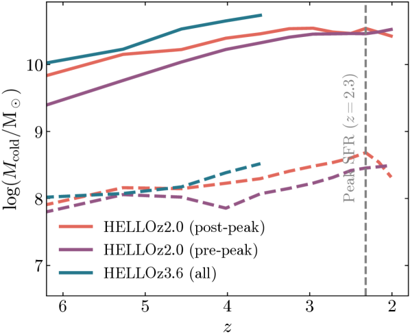
Figure 12: Median cold ($T<15000$ K) gas mass time evolution for HELLOz2.0 post-peak (orange), HELLOz2.0 pre-peak (purple), and HELLOz3.6 (turquoise) galaxies since $z=6$. The continuous curves represent $M_{\mathrm{cold}}$ within 0.2 $R_{200}$, while the dashed ones are for the central cold gas mass within 1 kpc. The grey dashed line indicates the epoch when the post-peak sample reaches its median peak SFR.

At $z=2$, both the pre-peak and post-peak galaxies have roughly the same amount of cold gas available, but with an opposite trend. While (central) cold gas mass is still increasing in the pre-peak sample, it is decreasing in the pre-peak sample after $z=2.3$, which corresponds to when post-peak galaxies reach their median peak SFR. At their final redshift, HELLOz3.6 galaxies possess roughly twice as much median cold gas within 20 per cent of ${{R_{200}}}$, but a similar central amount compared to HELLOz2.0. A list of the exact values for each galaxy at the final redshift can be found in Appendix A.

Gas temperature is only half of the story in the ability of a galaxy to form stars; the gas also needs to reach a density of $n\geq 10$ cm^-1 in our case. Fig. 13 shows the distribution of gas mass within density (left panels) and temperature (right panels) bins, calculated within $0.2\,{{R_{200}}}$. The upper row compares HELLOz2.0 pre- and post-peak, while the lower one compares between the whole of HELLOz2.0 and HELLOz3.0 samples. In each panel, the thick lines delineate the median of the lighter semi-transparent lines, representing individual galaxies, the vertical black line denotes where the threshold in $n$ and $T$ for star formation is, and the yellow star indicates the region (above or below the respective threshold) where star formation is allowed to take place. Each curve is computed from their respective final snapshots.

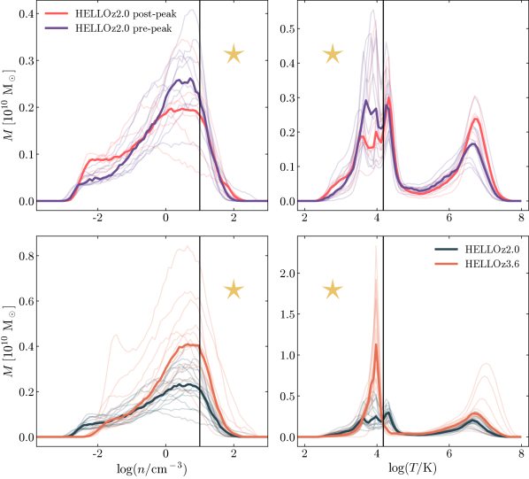
Figure 13: Gas distributions of our simulations, binned in log-density (left column) and log-temperature (right column). The upper row compares HELLOz2.0 post-peak (red) with pre-peak (purple) galaxies, and the lower row compares the whole samples of HELLOz2.0 (dark green) with HELLOz3.6 (brown). Translucent curves represent individual galaxies and their median is plotted as a solid opaque curve. In each panel, the vertical black line indicates the location of the density and temperature threshold, and the yellow star indicates the values allowing star formation.

Starting with temperature on the right, the two panels confirm what we observed in Fig. 12, namely that post-peak galaxies show slightly less, but a similar amount of available cold gas to form stars at the final redshift. On the other hand, simulations at $z=3.6$ have clearly more cold gas at their disposal. Individually, there is an apparent distinction between HELLOz2.0 and HELLOz3.6, meaning that not only the median values are different, but also individual galaxies at $z=3.6$ have systematically more cold gas than their $z=2.0$ counterpart. This is unlike pre- and post-peak, which display more overlapping curves.

Moving to the distribution in density (left panels), the findings are analogous between both redshifts. HELLOz3.6 reveals a higher amount of dense gas, both individually and in the median. At $z=2.0$, however, the pre- and post-peak galaxies exhibit an overlapping median distribution of dense gas. Interestingly though for densities $1\mathrel{\hbox{\hbox to0.0pt{\hbox{\lower 4.0pt\hbox{$\sim$}}\hss}\hbox{$<$}}}n\mathrel{\hbox{\hbox to0.0pt{\hbox{\lower 4.0pt\hbox{$\sim$}}\hss}\hbox{$<$}}}10$ cm^-1, the median distributions show the largest disparities, indicating that pre-peak galaxies contain larger reservoirs of gas close to the star formation density threshold, thus allowing them to potentially sustain further SFR growth relative to post-peak galaxies.

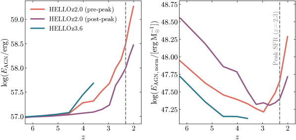
Figure 14: The left panel displays the median cumulative AGN feedback energy time evolution for HELLOz2.0 post-peak (orange), HELLOz2.0 pre-peak (purple), and HELLOz3.6 (turquoise) galaxies since $z=6$. The grey dashed line indicates the epoch when the post-peak sample reaches its median peak SFR. The right panel shows the same quantity normalised by the stellar mass. The normalisation is applied to each galaxy prior to computing the median.

5.2 AGN feedback

We now turn our attention towards the energy released by a central AGN and investigate if we can observe signs of its potential role in regulating its host galaxy’s SFR. Fig. 14 contains the time evolution of the median cumulative AGN feedback energy released (left) and the same quantity normalised by the stellar mass at each redshift (right), i.e., $E_{\mathrm{AGN,norm}}(z)=E_{\mathrm{AGN}}(z)/M_{\star}(z)$. The colour code in both panels follows the same convention as Fig. 12. The three curves in the left panel exhibit a similar evolution, with a sudden exponential growth beginning between $z\sim 4.5$ and $z\sim 3$. At their respective final redshifts, HELLOz3.6 galaxies have released a total of $\log(E_{\mathrm{AGN}}/\mathrm{erg})=57.7$ of AGN feedback energy, which is less than their counterparts at z=2.0, who reach $\log(E_{\mathrm{AGN}}/\mathrm{erg})=58.5$ and $\log(E_{\mathrm{AGN}}/\mathrm{erg})=59.3$ for pre- and post-peak samples, respectively.

When normalising by stellar mass (right panel), the following picture emerges. During the initial phase of their evolution, the stellar mass growth of galaxies dominates over BH growth until the trend is reverted at a turnaround redshift of $z\sim 4$ for HELLOz3.6 and $z\sim 3$ for HELLOz2.0 galaxies. In the second phase, BH growth dominates relative to stellar mass. Notably unlike the samples at $z=2$, HELLOz3.6 does not exhibit a dominating BH growth in its median curve yet. Nevertheless, we looked at the most massive simulations individually, and their curve has indeed reverted. We are therefore confident in our prediction that overall, the HELLOz3.6 galaxies would display a similar U-shaped curve if allowed to evolve further.

The right panel of Fig. 14 suggests two main results. First, assuming AGN feedback is (at least in some part) responsible for the quenching of galaxies, the value of $E_{\mathrm{AGN,norm}}$ alone is not sufficient to predict if a galaxy’s SFR is about to weaken. Indeed, the median value of $E_{\mathrm{AGN,norm}}$ for HELLOz2.0 at $z=6$ is similar to the value at $z=2.3$, which corresponds to peak SFR, having thus increased during this time interval. Second, given that both curves of pre- and post-peak galaxies have already reverted, despite only the post-peak sample showing a decreasing SFR in the last few hundreds of Myr, we believe that the turnover in the $E_{\mathrm{AGN,norm}}$ evolution acts as a precursor to a slowing SFR and eventually quenching. In other words, we predict that on average, the pre-peak sample is about to meet a similar fate as the post-peak one.

Fig. 15 displays the relative amount of feedback energy released by the AGN with respect to the total feedback (AGN plus stars) between each snapshot, i.e., in $\sim$200 Myr timesteps. The HELLOz2.0 post-peak galaxies are represented as orange circles, HELLOz2.0 pre-peak as purple squares, and HELLOz3.6 as turquoise triangles, respectively. We purposefully avoid using a solid curve as before, to emphasise that Fig. 15 does not show the cumulative relative energy, but rather the energy emitted during each snapshot.

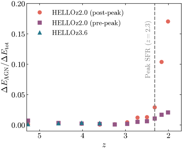
Figure 15: Fraction of energy released by the AGN relative to the total energy made up of AGNs, ESF, and SNe, in each snapshot. HELLOz2.0 post-peak galaxies are represented as orange circles, HELLOz2.0 pre-peak as purple squares, and HELLOz3.6 as turquoise triangles, respectively. The dashed grey line indicates where post-peak galaxies reach their median peak SFR at $z=2.3$.

In our analysis, the interplay between stellar and AGN feedback arises as a pivotal factor in the energetic dynamics of galaxy evolution. Up to $z=3$, stellar feedback is the predominant contributor to the energy output, completely overshadowing AGN feedback. However, a notable shift occurs post $z=3$, where AGN feedback begins to assert a more significant role. This trend is particularly pronounced in the HELLOz2.0 post-peak galaxies, where AGN feedback surges from 3 per cent to 17 per cent by $z=2$. This uptick in AGN activity is linked to the concurrent decline in SFR, a dual phenomenon that underscores the complex interdependencies within galactic systems.

Although the increase in AGN feedback is less pronounced in pre-peak galaxies, it is noteworthy that its contribution steadily grows, even outpacing the rising SFR. This observation is consistent with the trends noted in the right panel of Fig. 14. Meanwhile, HELLOz3.6 galaxies are so efficient at forming stars that the fraction $\Delta E_{\mathrm{A}GN}$ relative to the total output $\Delta E_{\mathrm{t}ot}$ remains negligible until the final redshift. Yet, the leveling off observed in the right panel of Fig. 14 suggests an impending shift in this trend, potentially aligning these galaxies with the evolutionary trajectory of HELLOz2.0 galaxies. It is important to emphasise that while AGN feedback may be quantitatively lesser in overall energy contribution compared to stellar feedback, its localised nature, concentrated at the galactic centre, implies a disproportional impact on the immediate surroundings.

A potential limitation of our study lies in the dependence of our results on the Bondi model of BH accretion, where $\dot{M}_{\bullet}\propto M_{\bullet}^{2}$ (see Eq. 4). As illustrated by Blank et al. (2019), BH mergers are the primary catalysts for substantial increases in BH mass at early times, thus allowing for significant accretion and the onset of runaway growth. This might be the reason behind the relatively late beginning of BH growth in HELLOz3.6 galaxies, which as a result, lack the time to accrete (and thus emit) as much as HELLOz2.0 BHs. Furthermore, Soliman et al. (2023) demonstrated by using NIHAO simulations that the choice of the accretion model can significantly affect the evolution of a galaxy. In the future, we are working on testing different implementations of AGN accretion and feedback (C. Cho et al. 2024, in prep.).

6 Summary and conclusion

In this paper, we presented HELLO, a new set of high-resolution cosmological zoom-in simulations for massive MW-type galaxies at final redshifts of $z=2$ and $z=3.6$, respectively. The hydrodynamics and sub-grid physics governing the evolution of these galaxies are identical to NIHAO (Wang et al., 2015; Blank et al., 2019) with the addition of LPF from Obreja et al. (2019) and a revised elemental feedback, as introduced by Buck et al. (2021). The HELLO sample used here consists of a total of 32 simulations with ${{M_{\star}}}\sim 10^{10-11}\,{\mathrm{M}}_{\astrosun}$ and $N_{\mathrm{part}}\sim 10^{6}$ within their respective virial radii. We summarise our results as follows:

1. Our simulations reproduce the high SFRs measured in SFGs at 2–3 Gyr after the Big Bang. Moreover, HELLOz2.0 galaxies show signs of a flattening slope above ${\log(M_{\star}/\mathrm{M}_{\odot})}\sim 10.5$ in the SFR–$M_{\star}$ plane, unlike their $z=3.6$ counterparts (Fig. 6).

2. HELLO galaxies are in good agreement with the SFR–$M_{\star}$ relation found by various authors in the literature (Schreiber et al., 2015; Tomczak et al., 2016; Barro et al., 2017), particularly at $z\sim 4$ where our simulations exhibit a remarkably tight distribution around the SFMS (Fig. 7). Both HELLOz2.0 and HELLOz3.6 samples show some tension with the relations found by Pearson et al. (2018).

3. Our study finds that HELLOz2.0 galaxies generally underpredict the size-mass relation observed for SFGs (van der Wel et al., 2014), especially at higher stellar masses where post-peak galaxies deviate significantly from the relation (Fig. 8). Possible reasons include relatively weaker stellar feedback with respect to $M_{\star}$ (McCarthy et al., 2012; Arora et al., 2023) and the onset of the quenching phase in post-peak galaxies.

4. HELLO simulations exhibit a consistent median size increase from $z\sim 8$ to $z\sim 3$, followed by a stabilization or contraction (Fig. 12). This size evolution overestimates effective radii compared to observed galaxies from the JWST (Ormerod et al., 2024). However, our curves represent the median track of individual galaxies and not similar mass ones at each redshift probed. A notable size compaction is observed in the post-peak sample between $3<z<2.3$, aligning with the peak SFR and followed by a modest expansion during the SFR decline, consistent with Wellons et al. (2015) and Tacchella et al. (2016).

5. Our study’s findings align with the general consensus of galaxy sizes correlating negatively with redshift at fixed $M_{\star}$ (Fig. 10). However, our results highlight a nuanced aspect: HELLO galaxies at higher redshifts are smaller up to a stellar mass of ${\log(M_{\star}/\mathrm{M}_{\odot})}\sim 10$, with the relationship becoming more complex beyond this mass threshold. This could suggest analogous evolutionary mechanisms across both samples.

6. HELLO galaxies closely match the central density relation for SFGs within 1 kpc (Barro et al., 2017), in terms of both slope and scatter (Fig. 11). However, the simulations tend to overpredict the effective surface density, particularly for post-peak galaxies, aligning more with the quiescent relation. This overprediction follows naturally from our smaller sizes, as summarised in (iii).

7. All samples exhibit a steady increase in cold gas mass on aggregate, with HELLOz2.0 beginning to saturate below $z\sim 3$ (Fig. 12). At $z=2$, pre-peak and post-peak galaxies have similar amounts of cold gas, but with contrasting trends: increasing in pre-peak and decreasing in post-peak galaxies after $z=2.3$, which coincides with the median peak SFR for post-peak simulations. HELLOz3.6 galaxies have about twice as much median cold gas mass overall as compared to HELLOz2.0 galaxies at their final redshift.

8. Gas density analyses show that HELLOz3.6 galaxies have a higher amount of dense gas suitable for star formation, both individually and on average (Fig. 13).

9. While stellar feedback dominates the feedback energy liberated, the central BHs of our galaxies have undergone substantial growth since $z\sim 4$ (Figs. 14 and 15). At their respective final redshifts, galaxies at $z=2$ have more massive BHs than their counterparts at $z=3.6$, with the post-peak sample having the most massive BHs.

A general picture materialises from our results, which we describe as follows. Beginning with galaxies at $z=2$, they undergo a relatively smooth progression along the SFMS, characterised by sustained SFR growth and cold gas accumulation. During this phase, galaxies expand in size until they begin to plateau below $z\sim 4$. Post-peak galaxies, which are generally the most massive, consistently exhibit higher SFRs and undergo a significant period of contraction until they reach their peak SFR around $z\sim 2.3$, coinciding with significant BH growth. As a result, this period witnesses the depletion of central gas, attributed to the central BH and stars consuming the gas, and in turn, emitting a substantial amount of energy, leading to a negative feedback loop at the heart of the declining SFR.

Conversely, pre-peak galaxies have yet to achieve their peak SFRs. While their size is seemingly reaching a saturation point, they do not display a reduction in central cold gas reserves and their AGNs activity is significantly less intense, as indicated by the lower feedback emission. Nonetheless, we postulate that these galaxies are merely trailing behind their post-peak counterparts and will eventually mirror the latter in a few hundred Myr, as indicated by their stellar masses and high SFRs (see, e.g. Peng et al., 2010).

Although HELLOz3.6 galaxies have not yet peaked, the trend in their size evolution suggests a probable onset of contraction and cessation of SFR growth in their near future, similar to the prediction for HELLOz2.0 pre-peak galaxies, unless their cold gas reservoirs continue to replenish at a rates that offset the effects of stellar and AGNs feedback. In both scenarios, however, our results indicate that despite similar stellar masses, our galaxies at $z=3.6$ are somewhat trailing behind HELLOz2.0 galaxies in their evolution, suggesting that there is more at play than merely a ‘transition’ stellar mass (Birnboim & Dekel, 2003; Kereš et al., 2005).

At $z=3.6$, galaxies possess larger reserves of cold and high-density gas, accounting for their higher SFRs. They additionally host less massive BHs, whose feedback is substantially weaker than galaxies at $z=2$. These differences could be attributed to the shorter cooling times prevalent at high redshift, allowing the gas to cool and reach the density threshold faster. The gas, in turn, actively forms stars rather than feeding the central AGN.

Our findings support the notion that AGN feedback is (partly) responsible for the quenching of galaxies. However, this does not preclude the simultaneous occurrence of intense AGNs activity and high SFRs in SFGs (Hopkins et al., 2006). Both post- and pre-peak galaxies exhibit comparable median SFRs at their final redshifts, but follow inverse trajectories. This implies that the exponential growth of central black holes and the ensuing feedback both precede the quenching process (Di Matteo et al., 2005; Springel et al., 2005).

As it is, the HELLO simulations represent a meaningful step in progress toward an improved understanding of the nature of galaxies at high redshifts, and its forthcoming improvements will help to further advance its capabilities.

Data availability

The data underlying this article will be shared on reasonable request to the corresponding author.

Appendix A HELLO quantities at their final redshift

Name	$N_{\mathrm{tot}}$	$N_{\mathrm{DM}}$	$N_{\star}$	$N_{\mathrm{gas}}$	$R_{200}$	$R_{\mathrm{e}}$	$M_{\mathrm{halo}}$	$M_{\mathrm{DM}}$	$M_{\star}$	$M_{\mathrm{gas}}$	$M_{\mathrm{cold}}$	$M_{\mathrm{cold},1}$	$M_{\bullet}$	$\mathrm{SFR}_{10}$	$\mathrm{SFR}_{100}$	$\Sigma_{1}$	$\Sigma_{\mathrm{e}}$	$\Delta\mathrm{ESF}$	$\Delta\mathrm{SNe\,II}$
							$\times 10^{12}$	$\times 10^{12}$	$\times 10^{10}$	$\times 10^{10}$	$\times 10^{12}$	$\times 10^{8}$	$\times 10^{6}$			$\times 10^{9}$	$\times 10^{9}$	$\times 10^{59}$	$\times 10^{57}$
					[a]	[a]	[b]	[b]	[b]	[b]	[b]	[b]	[b]	[c]	[c]	[d]	[d]	[e]	[e]
g3.08e12	1,943,368	732,154	752,300	458,914	142	1.5	2.84	2.48	10.09	7.31	2.60	2.07	34.42	55	60	6.64	5.43	3.73	2.87
g3.09e12	2,058,093	758,531	836,846	462,716	144	2.4	2.94	2.57	11.33	7.26	2.47	0.00	74.07	68	65	5.56	3.07	4.07	3.14
g3.00e12	1,501,948	626,696	433,000	442,252	135	1.9	2.43	2.12	5.91	8.33	3.45	4.11	0.51	99	87	2.91	2.23	4.13	3.18
g3.20e12	1,693,806	694,672	456,825	542,309	140	3.3	2.72	2.35	5.69	9.27	4.35	2.61	3.31	81	75	2.37	0.99	3.92	3.02
g2.75e12	1,778,286	624,856	720,877	432,553	135	2.3	2.45	2.12	9.74	8.77	4.34	2.08	24.14	66	66	7.82	3.84	3.96	3.05
g3.03e12	1,250,411	426,342	548,685	275,384	119	2.3	1.67	1.44	7.55	5.69	2.35	2.78	5.56	54	66	5.12	2.48	3.85	2.96
g3.01e12	1,729,071	683,692	563,963	481,416	139	1.7	2.66	2.32	7.67	7.41	2.72	4.36	3.02	84	83	5.94	4.14	4.80	3.69
g2.29e12	1,333,337	460,720	543,304	329,313	122	2.8	1.81	1.56	7.53	7.71	3.19	3.79	4.94	95	81	4.39	1.73	4.30	3.31
g3.35e12	964,316	441,712	175,744	346,860	120	2.1	1.72	1.50	2.37	6.69	3.25	2.71	1.05	53	47	0.93	0.67	2.47	1.90
g3.31e12	1,449,371	594,285	408,855	446,231	133	1.6	2.32	2.01	5.27	8.21	3.79	5.05	13.40	79	52	3.94	2.99	3.13	2.41
g3.25e12	1,643,064	674,577	412,909	555,578	139	3.1	2.65	2.29	4.09	8.11	4.55	2.26	1.19	58	46	1.68	0.72	2.67	2.06
g3.38e12	2,014,002	787,483	639,957	586,562	146	1.5	3.08	2.67	8.09	9.86	3.68	9.65	4.70	106	85	6.26	4.51	5.91	4.55
g3.36e12	1,209,250	529,555	251,774	427,921	128	2.0	2.08	1.79	3.14	4.43	1.95	2.16	2.22	31	35	1.55	1.14	1.85	1.42
g2.83e12	1,551,228	592,464	523,384	435,380	133	2.5	2.32	2.01	6.57	5.75	2.24	3.32	3.44	86	63	3.19	1.63	3.39	2.61
g2.63e12	1,682,819	596,827	661,422	424,570	133	3.1	2.35	2.02	9.01	7.85	3.34	3.12	1.36	93	93	3.14	1.67	5.14	3.96
g3.04e12	1,997,107	774,655	710,292	512,160	145	2.2	3.01	2.63	9.50	8.10	2.82	2.03	17.25	103	102	5.14	3.11	6.00	4.62
g2.91e12	1,445,948	541,666	542,915	361,367	129	1.3	2.11	1.84	7.29	4.33	1.36	4.22	13.63	40	40	6.01	5.51	2.38	1.83
g2.47e12	1,259,900	567,753	247,017	445,130	87	2.2	2.21	1.92	3.39	8.16	3.94	2.61	0.44	121	104	1.22	0.92	5.09	3.91
g2.40e12	1,231,536	577,171	123,812	530,553	88	2.6	2.29	1.96	0.62	5.16	3.43	1.09	0.16	27	21	0.18	0.12	1.01	0.77
g2.69e12	1,493,797	650,082	332,760	510,955	91	2.3	2.54	2.20	4.53	10.95	5.47	4.14	0.28	178	158	1.89	1.17	7.13	5.49
g3.76e12	1,998,769	910,838	298,900	789,031	102	2.0	3.58	3.09	3.45	12.28	6.08	3.31	0.54	146	127	1.26	0.89	6.31	4.85
g4.58e12	1,616,009	662,886	417,102	536,021	92	2.6	2.60	2.25	5.86	11.22	5.44	4.89	1.12	165	149	3.65	1.60	7.66	5.89
g2.71e12	1,216,000	490,095	304,633	421,272	84	2.5	1.98	1.70	4.35	9.75	4.76	3.72	0.64	159	123	1.92	1.07	6.44	4.95
g2.49e12	1,427,551	647,600	227,010	552,941	91	2.2	2.55	2.19	2.99	9.72	4.83	2.76	0.14	113	108	1.30	0.87	5.13	3.95
g2.51e12	1,529,843	635,272	338,985	555,586	91	2.0	2.52	2.15	2.61	6.57	3.89	2.75	0.39	62	59	1.68	1.02	3.07	2.36
g7.37e12	3,526,490	1,465,334	866,819	1,194,337	120	2.2	5.76	4.97	11.64	20.65	8.87	11.06	1.42	407	355	6.05	3.14	16.88	12.99
g2.32e12	1,218,031	486,245	340,064	391,722	83	2.1	1.91	1.65	4.93	8.47	4.19	4.48	0.81	124	125	2.95	1.69	6.94	5.34
g2.96e12	1,605,548	716,314	258,236	630,998	95	2.8	2.84	2.45	3.43	12.71	6.63	2.10	0.26	159	122	0.99	0.62	5.83	4.48
g7.97e12	3,546,175	1,487,662	755,426	1,303,087	121	1.2	5.89	5.04	7.12	13.80	6.76	10.00	3.04	183	169	7.22	6.02	9.03	6.95
g9.20e12	5,318,120	2,230,919	1,317,484	1,769,717	138	2.4	8.74	7.56	14.15	25.68	10.61	1.21	66.69	351	352	9.39	4.07	19.82	15.25

Table 2: Simulation quantities for HELLOz2.0 and HELLOz3.6 galaxies at their final redshifts of $z=2$ (top) and $z=3.6$ (bottom), respectively. Columns from left to right: galaxy name, total number of particles ($N_{\mathrm{tot}}$), number of DM particles ($N_{\textrm{DM}}$), number of star particles ($N_{\star}$), number of gas particles ($N_{\mathrm{gas}}$), virial radius (${{R_{200}}}$), effective radius (${{R_{\mathrm{e}}}}$), halo mass ($M_{\mathrm{halo}}$), DM mass ($M_{\mathrm{DM}}$), stellar mass ($M_{\star}$), gas mass ($M_{\mathrm{gas}}$), cold gas mass ($M_{\mathrm{cold}}$), cold gas mass within 1 kpc ($M_{\mathrm{cold,1}}$), BH mass ($M_{\bullet}$), SFR averaged over the last 10 Myr (SFR₁₀), SFR averaged over the last 100 Myr (SFR₁₀₀), stellar surface density within 1 kpc ($\Sigma_{1}$), effective stellar surface density ($\Sigma_{\mathrm{e}}$), ESF energy released during the last 200 Myr ($\Delta$ESF), and SNe II energy released during the last 200 Myr ($\Delta$SNe II).
The different numbers of particles, as well as $M_{\mathrm{halo}}$ and $M_{\mathrm{DM}}$, are computed within $R_{200}$, while baryonic quantities are computed within $0.2\,{{R_{200}}}$, unless otherwise specified by the indices ‘1’ or ‘e.’
Units: [a] $\equiv$ [kpc], [b] $\equiv$ [${\mathrm{M}}_{\astrosun}$], [c] $\equiv$ [${\mathrm{M}}_{\astrosun}\,\mathrm{yr}^{-1}$], [d] $\equiv$ [${\mathrm{M}}_{\astrosun}\,\mathrm{kpc}^{-2}$], and [e] $\equiv$ [erg].

Appendix B Choice of each galactic radius

In order to calculate various baryonic quantities such as $M_{\star}$, $M_{\mathrm{gas}}$, or SFR, we need to define the edges of the galaxy. Ideally, the chosen rule should i) be simple and consistent and ii) allow for as fair a comparison with observations as possible. In this paper we chose a sphere enclosing 20 per cent of $R_{200}$ as our galactic radius for calculating galactic baryonic properties. While somewhat arbitrary, this choice offers consistency across all galaxies within our sample, as well as with NIHAO and other simulations (Wang et al., 2015; Tacchella et al., 2016). Stevens et al. (2014) tested different methods defining the galactic edge in simulations and, while they advise against using a fraction of the virial radius, they found that the chosen technique does not significantly affect comparisons with observed scaling relations. It should also be highlighted that observations are not devoid of similar debates and different methods can lead to different results as well (Bernardi et al., 2013).

One caveat with our choice is that at high-$z$, our galaxies have fairly large halos (${{R_{200}}}\mathrel{\hbox{\hbox to0.0pt{\hbox{\lower 4.0pt\hbox{$\sim$}}\hss}\hbox{$>$}}}100$ kpc) relative to their size. In addition, it is apparent from Fig. 2 that the direct surroundings of some galaxies is rather chaotic with the presence of close-by satellites about to merge. We therefore compare the values we obtain for $M_{\star}$, when taking $0.1\,{{R_{200}}}$ with respect to our fiducial $0.2\,{{R_{200}}}$, and make sure that $M_{\star}$ does not vary by more than $\sim$10 per cent at the final redshift. We also control that the variation in $R_{\mathrm{e}}$, $\Sigma_{\mathrm{e}}$, and SFR also remains within these bounds. The results are visible in the following Table 3.

Name	$z_{\mathrm{final}}$	$\Delta M_{\star}$	$\Delta{{R_{\mathrm{e}}}}$	$\Delta{{\Sigma_{\mathrm{e}}}}$	$\Delta\mathrm{SFR}_{100}$
g3.08e12	2.0	$-$1.2	$-$1.4	0.9	$-$0.5
g3.09e12	2.0	$-$2.2	0.1	$-$0.1	0.0
g3.00e12	2.0	$-$4.1	$-$2.4	1.8	$-$0.5
g3.20e12	2.0	$-$2.2	$-$1.6	1.8	$-$0.4
g2.75e12	2.0	$-$1.8	$-$2.3	2.8	$-$0.9
g3.03e12	2.0	$-$2.2	$-$1.7	2.0	0.0
g3.01e12	2.0	$-$1.2	$-$0.1	0.1	$-$0.2
g2.29e12	2.0	$-$1.9	$-$1.3	1.5	$-$0.3
g3.35e12	2.0	$-$9.0	$-$6.5	5.4	$-$0.9
g3.31e12	2.0	$-$4.0	$-$5.1	4.2	$-$2.0
g3.25e12	2.0	$-$7.9	$-$6.6	7.9	$-$4.8
g3.38e12	2.0	$-$13.8	$-$11.8	12.8	$-$1.6
g3.36e12	2.0	$-$1.2	0.0	0.0	$-$0.6
g2.83e12	2.0	$-$10.6	$-$10.0	9.6	$-$12.3
g2.63e12	2.0	$-$1.5	$-$0.1	0.1	0.0
g3.04e12	2.0	$-$2.1	$-$0.9	0.8	$-$0.1
g2.91e12	2.0	$-$0.3	$-$0.3	0.1	0.0
g2.47e12	3.6	$-$3.9	$-$1.6	1.2	$-$0.9
g2.40e12	3.6	$-$5.5	$-$4.1	3.2	$-$4.6
g2.69e12	3.6	$-$9.1	$-$6.3	5.7	$-$1.1
g3.76e12	3.6	$-$8.1	$-$4.1	3.4	$-$1.3
g4.36e12	3.6	$-$30.8	$-$39.1	73.2	$-$26.0
g4.58e12	3.6	$-$4.7	$-$3.5	4.3	$-$0.9
g2.71e12	3.6	$-$4.3	$-$2.0	1.8	$-$0.9
g2.49e12	3.6	$-$5.3	$-$3.3	2.8	$-$1.2
g2.51e12	3.6	$-$2.0	$-$1.7	1.7	$-$0.9
g7.37e12	3.6	$-$6.0	$-$6.2	6.8	$-$2.2
g2.32e12	3.6	$-$2.5	$-$0.8	0.8	$-$0.4
g2.96e12	3.6	$-$11.7	$-$9.9	9.0	$-$6.6
g7.97e12	3.6	$-$4.8	$-$7.7	7.8	$-$3.6
g9.20e12	3.6	$-$6.4	$-$4.5	5.6	$-$1.8
g9.85e12	3.6	$-$39.5	$-$64.4	387.1	$-$37.7

Table 3: Columns from left to right: galaxy name, final redshift, and percentage differences in $M_{\star}$, $R_{\mathrm{e}}$, $\Sigma_{\mathrm{e}}$, and SFR₁₀₀, when using $0.1\,{{R_{200}}}$ instead of the fiducial $0.2\,{{R_{200}}}$ as each galaxy’s defined radius. The two galaxies in bold were not used in this work.

We highlighted the two galaxies that we did not use in this paper due to the significant difference in $M_{\star}$ (and all other quantities) when reducing the galactic radius to $0.1\,{{R_{200}}}$. For completeness, we show their stellar surface density maps in Fig. 16. These maps are similar to Fig. 2 where, in this case, the outer dashed and inner dotted circles represent $0.2\,{{R_{200}}}$ and $0.1\,{{R_{200}}}$, respectively. As illustrated in Table 3, these two merger events significantly affected the calculated stellar quantities with respect to each galaxy’s chosen edge. We thus excluded them from this paper.

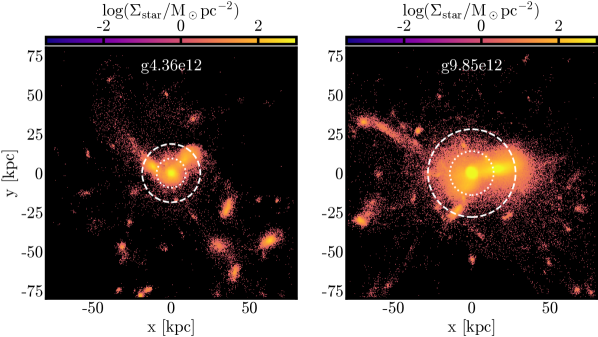
Figure 16: Stellar surface density maps viewed face-on for g4.36e12 and g9.85e12 that were excluded from this work. The white dashed and dotted circles indicate a galactic radius of $0.2\,{{R_{200}}}$ and $0.1\,{{R_{200}}}$, respectively.

Appendix C Computing the energy from stellar feedback

In what follows we detail the methodology employed to calculate the energies associated with ESF and SNe feedback. We calculate both quantities separately during each snapshot before combining them to obtain the total stellar feedback energy.

The energy release during each simulation snapshot is calculated for stars formed within specific time intervals relative to the snapshots. For a given snapshot s at cosmic age $t$ in Myr, the relevant stars are those formed in the time interval $t_{\mathrm{s}-1}-4<t_{\mathrm{form}}<t_{\mathrm{s}}-4$, where $t_{\mathrm{form}}$ is the age of the universe when the star particle was formed and the subtraction by 4 refers to the 4 Myr during which young stars release ESF and before which the eligible stars explode as SNe. For the calculation, we assume that both feedback energies are released at once 4 Myr after the stellar particle was formed.

Once only the relevant stars are selected, the amount ESF ejected during one snapshot is calculated as:

$$\Delta\mathrm{ESF}=\epsilon_{\mathrm{ESF}}\cdot 2\times 10^{50}\,\mathrm{erg/{\mathrm{M}}_{\astrosun}}\,\cdot M_{\mathrm{form}},$$ (7)

where $2\times 10^{50}$ is the amount of energy in erg released per solar mass formed ($M_{\mathrm{form}}$) from SNe and $\epsilon_{\mathrm{ESF}}=0.13$ is the fraction of this energy ejected as isotropic thermal energy.

The SN feedback energy is computed based on the number of stars within the mass range 8-40 ${\mathrm{M}}_{\astrosun}$ that are expected to explode as SN II, expressed as $N_{\mathrm{SN}}$. This is determined by integrating the Chabrier IMF (Chabrier, 2003) over the specified mass range, scaled by the total $M_{\mathrm{form}}$. The SN feedback energy is then given by:

$$\Delta\mathrm{SN}=\epsilon_{\mathrm{SN}}\cdot N_{\mathrm{SN}}\cdot 10^{51}\,\mathrm{erg/SN}.$$ (8)

References

- Arora et al. (2023) Arora N., Courteau S., Stone C., Macciò A. V., 2023, MNRAS, 522, 1208
- Bagley et al. (2023) Bagley M. B., et al., 2023, ApJ, 946, L12
- Barro et al. (2017) Barro G., et al., 2017, ApJ, 840, 47
- Behroozi et al. (2013) Behroozi P. S., Wechsler R. H., Conroy C., 2013, ApJ, 770, 57
- Bell (2008) Bell E. F., 2008, ApJ, 682, 355
- Bernardi et al. (2013) Bernardi M., Meert A., Sheth R. K., Vikram V., Huertas-Company M., Mei S., Shankar F., 2013, MNRAS, 436, 697
- Bernhard et al. (2016) Bernhard E., Mullaney J. R., Daddi E., Ciesla L., Schreiber C., 2016, MNRAS, 460, 902
- Bertschinger (2001) Bertschinger E., 2001, ApJS, 137, 1
- Birnboim & Dekel (2003) Birnboim Y., Dekel A., 2003, MNRAS, 345, 349
- Blank et al. (2019) Blank M., Macciò A. V., Dutton A. A., Obreja A., 2019, MNRAS, 487, 5476
- Blank et al. (2021) Blank M., Meier L. E., Macciò A. V., Dutton A. A., Dixon K. L., Soliman N. H., Kang X., 2021, MNRAS, 500, 1414
- Bondi (1952) Bondi H., 1952, MNRAS, 112, 195
- Brammer et al. (2012) Brammer G. B., et al., 2012, ApJS, 200, 13
- Brinchmann et al. (2004) Brinchmann J., Charlot S., White S. D. M., Tremonti C., Kauffmann G., Heckman T., Brinkmann J., 2004, MNRAS, 351, 1151
- Buck et al. (2019) Buck T., Macciò A. V., Dutton A. A., Obreja A., Frings J., 2019, MNRAS, 483, 1314
- Buck et al. (2021) Buck T., Rybizki J., Buder S., Obreja A., Macciò A. V., Pfrommer C., Steinmetz M., Ness M., 2021, MNRAS, 508, 3365
- Buitrago et al. (2008) Buitrago F., Trujillo I., Conselice C. J., Bouwens R. J., Dickinson M., Yan H., 2008, ApJ, 687, L61
- Bundy et al. (2015) Bundy K., et al., 2015, ApJ, 798, 7
- Ceverino et al. (2014) Ceverino D., Klypin A., Klimek E. S., Trujillo-Gomez S., Churchill C. W., Primack J., Dekel A., 2014, MNRAS, 442, 1545
- Chabrier (2003) Chabrier G., 2003, PASP, 115, 763
- Cheung et al. (2012) Cheung E., et al., 2012, ApJ, 760, 131
- Chieffi & Limongi (2004) Chieffi A., Limongi M., 2004, ApJ, 608, 405
- Comerford et al. (2020) Comerford J. M., et al., 2020, ApJ, 901, 159
- Costa et al. (2018) Costa T., Rosdahl J., Sijacki D., Haehnelt M. G., 2018, MNRAS, 479, 2079
- Crain et al. (2015) Crain R. A., et al., 2015, MNRAS, 450, 1937
- Daddi et al. (2007) Daddi E., et al., 2007, ApJ, 670, 156
- Dahmer-Hahn et al. (2022) Dahmer-Hahn L. G., et al., 2022, MNRAS, 509, 4653
- Dekel & Birnboim (2006) Dekel A., Birnboim Y., 2006, MNRAS, 368, 2
- Di Matteo et al. (2005) Di Matteo T., Springel V., Hernquist L., 2005, Nature, 433, 604
- Dutton et al. (2017) Dutton A. A., et al., 2017, MNRAS, 467, 4937
- Dutton et al. (2020) Dutton A. A., Buck T., Macciò A. V., Dixon K. L., Blank M., Obreja A., 2020, MNRAS, 499, 2648
- Eddington (1921) Eddington A. S., 1921, Zeitschrift fur Physik, 7, 351
- Elbaz et al. (2007) Elbaz D., et al., 2007, A&A, 468, 33
- Ellison et al. (2016) Ellison S. L., Teimoorinia H., Rosario D. J., Mendel J. T., 2016, MNRAS, 458, L34
- Fang et al. (2013) Fang J. J., Faber S. M., Koo D. C., Dekel A., 2013, ApJ, 776, 63
- Faucher-Giguère et al. (2009) Faucher-Giguère C.-A., Lidz A., Zaldarriaga M., Hernquist L., 2009, ApJ, 703, 1416
- Ferland et al. (1998) Ferland G. J., Korista K. T., Verner D. A., Ferguson J. W., Kingdon J. B., Verner E. M., 1998, PASP, 110, 761
- Finkelstein et al. (2017) Finkelstein S. L., et al., 2017, The Cosmic Evolution Early Release Science (CEERS) Survey, JWST Proposal ID 1345. Cycle 0 Early Release Science
- Finkelstein et al. (2023) Finkelstein S. L., et al., 2023, ApJ, 946, L13
- Förster Schreiber & Wuyts (2020) Förster Schreiber N. M., Wuyts S., 2020, ARA&A, 58, 661
- Furlong et al. (2017) Furlong M., et al., 2017, MNRAS, 465, 722
- Gardner et al. (2006) Gardner J. P., et al., 2006, Space Sci. Rev., 123, 485
- Genel et al. (2014) Genel S., et al., 2014, MNRAS, 445, 175
- Gill et al. (2004) Gill S. P. D., Knebe A., Gibson B. K., 2004, MNRAS, 351, 399
- Grogin et al. (2011) Grogin N. A., et al., 2011, ApJS, 197, 35
- Gruppioni et al. (2013) Gruppioni C., et al., 2013, MNRAS, 432, 23
- Guo et al. (2013) Guo Y., et al., 2013, ApJS, 207, 24
- Haardt & Madau (1996) Haardt F., Madau P., 1996, ApJ, 461, 20
- Hardcastle et al. (2013) Hardcastle M. J., et al., 2013, MNRAS, 429, 2407
- Hopkins et al. (2006) Hopkins P. F., Hernquist L., Cox T. J., Di Matteo T., Robertson B., Springel V., 2006, ApJS, 163, 1
- Hopkins et al. (2018) Hopkins P. F., et al., 2018, MNRAS, 480, 800
- Juneau et al. (2013) Juneau S., et al., 2013, ApJ, 764, 176
- Kannan et al. (2014) Kannan R., Stinson G. S., Macciò A. V., Brook C., Weinmann S. M., Wadsley J., Couchman H. M. P., 2014, MNRAS, 437, 3529
- Kannan et al. (2016) Kannan R., Vogelsberger M., Stinson G. S., Hennawi J. F., Marinacci F., Springel V., Macciò A. V., 2016, MNRAS, 458, 2516
- Karakas & Lugaro (2016) Karakas A. I., Lugaro M., 2016, ApJ, 825, 26
- Kennicutt (1998) Kennicutt Robert C. J., 1998, ApJ, 498, 541
- Kereš et al. (2005) Kereš D., Katz N., Weinberg D. H., Davé R., 2005, MNRAS, 363, 2
- Knollmann & Knebe (2009) Knollmann S. R., Knebe A., 2009, ApJS, 182, 608
- Lang et al. (2014) Lang P., et al., 2014, ApJ, 788, 11
- Le Floc’h et al. (2005) Le Floc’h E., et al., 2005, ApJ, 632, 169
- Lee et al. (2015) Lee N., et al., 2015, ApJ, 801, 80
- Leslie et al. (2016) Leslie S. K., Kewley L. J., Sanders D. B., Lee N., 2016, MNRAS, 455, L82
- Ma et al. (2018) Ma X., et al., 2018, MNRAS, 477, 219
- Macciò et al. (2016) Macciò A. V., Udrescu S. M., Dutton A. A., Obreja A., Wang L., Stinson G. R., Kang X., 2016, MNRAS, 463, L69
- Macciò et al. (2020) Macciò A. V., Crespi S., Blank M., Kang X., 2020, MNRAS, 495, L46
- Madau & Dickinson (2014) Madau P., Dickinson M., 2014, ARA&A, 52, 415
- Martig et al. (2009) Martig M., Bournaud F., Teyssier R., Dekel A., 2009, ApJ, 707, 250
- McCarthy et al. (2012) McCarthy I. G., Schaye J., Font A. S., Theuns T., Frenk C. S., Crain R. A., Dalla Vecchia C., 2012, MNRAS, 427, 379
- McNamara & Nulsen (2007) McNamara B. R., Nulsen P. E. J., 2007, ARA&A, 45, 117
- Moster et al. (2013) Moster B. P., Naab T., White S. D. M., 2013, MNRAS, 428, 3121
- Neichel et al. (2018) Neichel B., Mouillet D., Gendron E., Correia C., Sauvage J. F., Fusco T., 2018, in Di Matteo P., Billebaud F., Herpin F., Lagarde N., Marquette J. B., Robin A., Venot O., eds, SF2A-2018: Proceedings of the Annual meeting of the French Society of Astronomy and Astrophysics. p. Di (arXiv:1812.06639), doi:10.48550/arXiv.1812.06639
- Noeske et al. (2007) Noeske K. G., et al., 2007, ApJ, 660, L43
- Obreja et al. (2019) Obreja A., Macciò A. V., Moster B., Udrescu S. M., Buck T., Kannan R., Dutton A. A., Blank M., 2019, MNRAS, 490, 1518
- Ormerod et al. (2024) Ormerod K., et al., 2024, MNRAS, 527, 6110
- Patel et al. (2013) Patel S. G., et al., 2013, ApJ, 766, 15
- Pearson et al. (2018) Pearson W. J., et al., 2018, A&A, 615, A146
- Peng et al. (2010) Peng Y.-j., et al., 2010, ApJ, 721, 193
- Penzo et al. (2014) Penzo C., Macciò A. V., Casarini L., Stinson G. S., Wadsley J., 2014, MNRAS, 442, 176
- Planck Collaboration et al. (2014) Planck Collaboration et al., 2014, A&A, 571, A16
- Pontzen et al. (2013) Pontzen A., Roškar R., Stinson G., Woods R., 2013, pynbody: N-Body/SPH analysis for python, Astrophysics Source Code Library, record ascl:1305.002
- Power et al. (2003) Power C., Navarro J. F., Jenkins A., Frenk C. S., White S. D. M., Springel V., Stadel J., Quinn T., 2003, MNRAS, 338, 14
- Rieke et al. (2023) Rieke M. J., et al., 2023, PASP, 135, 028001
- Rybizki et al. (2017) Rybizki J., Just A., Rix H.-W., 2017, A&A, 605, A59
- Salpeter (1964) Salpeter E. E., 1964, ApJ, 140, 796
- Schaye et al. (2015) Schaye J., et al., 2015, MNRAS, 446, 521
- Schiminovich et al. (2005) Schiminovich D., et al., 2005, ApJ, 619, L47
- Schiminovich et al. (2007) Schiminovich D., et al., 2007, ApJS, 173, 315
- Schmidt (1959) Schmidt M., 1959, ApJ, 129, 243
- Schreiber et al. (2015) Schreiber C., et al., 2015, A&A, 575, A74
- Seitenzahl et al. (2013) Seitenzahl I. R., et al., 2013, MNRAS, 429, 1156
- Skidmore et al. (2015) Skidmore W., TMT International Science Development Teams Science Advisory Committee T., 2015, Research in Astronomy and Astrophysics, 15, 1945
- Soliman et al. (2023) Soliman N. H., Macciò A. V., Blank M., 2023, MNRAS, 525, 12
- Sparre et al. (2015) Sparre M., et al., 2015, MNRAS, 447, 3548
- Speagle et al. (2014) Speagle J. S., Steinhardt C. L., Capak P. L., Silverman J. D., 2014, ApJS, 214, 15
- Springel et al. (2005) Springel V., Di Matteo T., Hernquist L., 2005, MNRAS, 361, 776
- Stadel (2001) Stadel J. G., 2001, PhD thesis, UNIVERSITY OF WASHINGTON
- Stadel (2013) Stadel J., 2013, PkdGRAV2: Parallel fast-multipole cosmological code, Astrophysics Source Code Library, record ascl:1305.005 (ascl:1305.005)
- Stevens et al. (2014) Stevens A. R. H., Martig M., Croton D. J., Feng Y., 2014, MNRAS, 445, 239
- Stinson et al. (2006) Stinson G., Seth A., Katz N., Wadsley J., Governato F., Quinn T., 2006, MNRAS, 373, 1074
- Stinson et al. (2013) Stinson G. S., Brook C., Macciò A. V., Wadsley J., Quinn T. R., Couchman H. M. P., 2013, MNRAS, 428, 129
- Tacchella et al. (2015) Tacchella S., et al., 2015, Science, 348, 314
- Tacchella et al. (2016) Tacchella S., Dekel A., Carollo C. M., Ceverino D., DeGraf C., Lapiner S., Mandelker N., Primack Joel R., 2016, MNRAS, 457, 2790
- Tomczak et al. (2016) Tomczak A. R., et al., 2016, ApJ, 817, 118
- Torrey et al. (2014) Torrey P., Vogelsberger M., Genel S., Sijacki D., Springel V., Hernquist L., 2014, MNRAS, 438, 1985
- Trujillo et al. (2007) Trujillo I., Conselice C. J., Bundy K., Cooper M. C., Eisenhardt P., Ellis R. S., 2007, MNRAS, 382, 109
- Valageas & Silk (1999) Valageas P., Silk J., 1999, A&A, 350, 725
- Vogelsberger et al. (2014) Vogelsberger M., et al., 2014, MNRAS, 444, 1518
- Wadsley et al. (2017) Wadsley J. W., Keller B. W., Quinn T. R., 2017, MNRAS, 471, 2357
- Wake et al. (2017) Wake D. A., et al., 2017, AJ, 154, 86
- Wang et al. (2015) Wang L., Dutton A. A., Stinson G. S., Macciò A. V., Penzo C., Kang X., Keller B. W., Wadsley J., 2015, MNRAS, 454, 83
- Waterval et al. (2022) Waterval S., et al., 2022, MNRAS, 514, 5307
- Wellons et al. (2015) Wellons S., et al., 2015, MNRAS, 449, 361
- Whitaker et al. (2014) Whitaker K. E., et al., 2014, ApJ, 795, 104
- Whitaker et al. (2017) Whitaker K. E., et al., 2017, ApJ, 838, 19
- Zhang et al. (2019) Zhang T., Liao S., Li M., Gao L., 2019, MNRAS, 487, 1227
- Zinger et al. (2020) Zinger E., et al., 2020, MNRAS, 499, 768
- van Dokkum et al. (2013) van Dokkum P. G., et al., 2013, ApJ, 771, L35
- van Dokkum et al. (2015) van Dokkum P. G., et al., 2015, ApJ, 813, 23
- van der Wel et al. (2012) van der Wel A., et al., 2012, ApJS, 203, 24
- van der Wel et al. (2014) van der Wel A., et al., 2014, ApJ, 788, 28