GLANCE – Gravitational Lensing Authenticator using Non-Modelled Cross-Correlation Exploration of Gravitational Wave Signals

Abstract

Gravitational lensing is the effect on a lightlike trajectory by the presence of matter, affecting its trajectory in spacetime. Gravitational lensing of gravitational waves can occur in geometric optics limit (when GW wavelength is much smaller than the Schwarzschild radius of the lens i.e. $\lambda_{GW}\ll$ R${}^{\rm sc}_{\rm lens}$, multiple images with different magnifications are formed) known as strong-lensing or in wave optics limit (when the wavelength of GW is larger than the Schwarzschild radius i.e. R${}^{\rm sc}_{\rm lens}$ $\lesssim\lambda_{GW}$, interfering signals produce beating pattern in the waveform envelope) known as micro-lensing. Currently, large sky-localization errors of GW sources and strong noise-PSD have barred us from evidencing lensed GWs. Considering this aspect, we have developed GLANCE, a novel technique to detect lensed GWs. We demonstrate that cross-correlation between the data pieces containing lensed signals shows a very specific trend. The strength of the cross-correlation signal can quantify the significance of the event(s) being lensed. Since lensing impacts the inference of the source parameters, primarily the luminosity distance for the strong lensing case, a joint parameter estimation of the source and lens-induced parameters is incorporated in GLANCE using a Bayesian framework. We applied our method to simulated strongly lensed data and we have shown that GLANCE not only can detect lensed GW signals but also can correctly infer the injected source and lens parameters even when one of the signals is below the match-filtered threshold SNR. This demonstrates the capability of GLANCE for a robust detection of lensed GW signal from noisy data.

1 Introduction

Gravitational waves (GWs) are the newest addition to the field of multi-messenger astrophysics. Since the first observation of the binary black-hole (BBH) merger on 14th September, 2015 (Abbott et al., 2016), there have been about 90 observations till their third observational run (Abbott et al., 2023b). These ripples in the fabric of spacetime provide us with a new way to understand the universe: inferring the Hubble constant (Abbott et al., 2023c) , population studies of merging compact binaries (Abbott et al., 2023a) , or testing the general theory of relativity (Abbott et al., 2021). Aside from its many differences with EM waves, GW also propagates in a light-like trajectory and they get gravitationally deflected by intervening matter according to the general theory of relativity. This phenomenon is known as the gravitational lensing of GW (Wang et al., 1996; Nakamura, 1998; Bartelmann, 2010; Dai et al., 2017). Owing to its kilometer-to-petameter range of wavelengths, GW provides us with new scales to observe the large-scale universe: from dwarf galaxies to galaxy clusters in different lensing regimes.

Figure 1: Outline for the strong lensing searches of GW using GLANCE. We can take the data from the GW observatories and extract the information about GW polarizations. We cross-correlate it with data from the same detector at some other time (or a different detector at almost the same time). The strength of the cross-correlation is measured by calculating its deviation from typical noise cross-correlation. For the significant events, to remove the lensing bias on the source parameters, we estimate the parameters of the source jointly with the lens-induced parameters.

Gravitational lensing of GW follows from Fermat’s principle of least time in presence of intervening matter in the trajectory of GW. Lensing can affect the spatial trajectory of GW leading to phase differences among GWs propagating along different paths. This creates an overall amplification of GW, upon interference. Much like ray optics and wave optics there are two distinct areas of lensing: (i) Geometric optics: in this limit, the Schwarzschild radius $(R_{s})$ of the intervening matter (the lens) is much larger than the wavelength $(\lambda)$ of the GW. Such cases are often known as strong lensing. Typically, such cases happen when km-sized GW passes near a galaxy or a galaxy cluster. (ii) Wave optics: in this limit, the Schwarzschild radius of the lens $(R_{s})$ is of comparable size or smaller than the wavelength $(\lambda)$ of the GW. This is known as the micro-lensing case. Due to the very different length scales involved here, the impact of gravitational lensed GWs can be studied in both geometric-optics and wave-optics regimes (or in their transition) depending on the lens mass and source masses. Multiband GW signal from compact objects covering nearly nHz to kHz signals can have different observable signatures in geometric optics and wave optics limit making it possible to explore cosmic structures of approximately $10^{14}$ M_⊙ to $10^{3}$ M_⊙ (Wambsganss, 2006; Bayer et al., 2023). In the absence of any luminous matter in the cosmic structures, lensing of GWs becomes the key method to study the electromagnetically undetectable dark matter halos over this mass range. The detection of lensed GW signals can lead to the measurement of plethora of science cases ranging from astrophysics to fundamental physics (Mukherjee et al., 2020b, a; Congedo & Taylor, 2019; Goyal et al., 2021; Basak et al., 2022; Ezquiaga et al., 2021; Mpetha et al., 2023; Balaudo et al., 2023; Çalışkan et al., 2023c; Narola et al., 2023).

The objective of the lensing project can be divided into three stages, as follows: Firstly, there is the detection of lensed GW signal, which is the main dealing of this paper then comes the inference of the source and lens-induced characterizations jointly and exploring their degeneracies and lastly given a handful of lensing observations we can study the properties of the lens from the data-driven approach.

In the current LIGO-VIRGO-KAGRA(LVK) sensitivity range (Abbott et al., 2018; Martynov et al., 2016; Buikema et al., 2020), observing a lensed GW is a very rare event, it has the probability of occurrence of a few parts in a thousand (0.1 - 0.6%) (Li et al., 2018; Mukherjee et al., 2021) (Diego et al., 2021). The lensing search by LVK on the O3 data led to no significant evidence of a lensed GW event (The LIGO Scientific Collaboration et al., 2023) using existing methods (Janquart et al., 2021; Lo & Magaña Hernandez, 2023; Wright & Hendry, 2022). A follow-up study on the O3 events did not bring up any significant observation of a lensing event so far (Janquart et al., 2023). With the improved detector network in the upcoming O5 run, it is expected to observe at least one lensed event based on our current understanding of the binary black hole(BBH) population, BBH merger rate and optical depth required for lensing. With the lensing observation chances increasing with improving detectors (Abbott et al., 2020), the necessity of a robust lensed GW finder seems of significant importance, which can detect these rare events confidently and accurately enough to validate them and isolate them from instrument noise.

Keeping this in mind, in this work, we have proposed a new and robust technique for the detection of lensed GW signals, GLANCE: Gravitational Lensing Authenticator using Non-modelled Cross-correlation Exploration. Fig. 1 shows the outline of the GLANCE framework. In a nutshell, we will use gravitational wave time-series data and extract the polarization information from it and cross-correlate this piece with another such piece. If the signals are cross-correlated in phase, we observe a peak in the cross-correlation signal. The deviation of this from typical noise cross-correlation helps us count an event as a lensing candidate, we call it as lensing signal-to-noise ratio (lensing SNR). For events above a certain threshold lensing SNR, we call it as a candidate for lensing and we then try to infer its source parameters. This is required to remove any false bias on the source parameters induced by lensing. We use both data pieces to infer the source and lens characterization jointly using the Bayesian framework. Application of cross-correlation technique on GW data analysis are applicable to search for beyond modelled non-GR signatures imprinted on GW (Dideron et al., 2023), stochastic GW background (Allen & Romano, 1999; Romano & Cornish, 2017), continuous GW searches (Dhurandhar et al., 2008) as well.

The following sections are organized as mentioned here: I) Motivation: In this section, we are going to discuss the current scenario of lensing and why a new pipeline is required to detect lensed GW signals. II) Basics of GW generation from CBC: In this section, we will find out how gravitational waves are generated from compact binary mergers and their propagation in free space III) Basics of Strong Lensing and Micro-lensing: In this section, how GW propagation is affected in presence of gravitating lens objects in different lensing regimes. IV) Mathematical Formulation: In this section, we formally describe the mathematical framework of our proposed technique to detect a lensed signal for both strong lensing and micro-lensing cases. V) Lens Parameter Estimation: In this section, we estimate the source parameters and lens characteristics imprinted on the signal for the strong lensing scenario after the detection of a lensed event.

2 Salient aspects of GLANCE

With increasing volume in the data from GW observatories and the chances of the observation of lensing increasing with upgraded GW detectors, the necessity of having good tools to analyze it and search for lensed signatures feels very important. In this prospect, we have developed a new method of detecting and characterizing the lensed GW signals that stands out from any current lensing finder technique. Since GW is a highly coherent waveburst and any alternation in phase, if there, is an observable in any data channel, the phase information is a clean probe to study lensing. Thus by applying cross-correlation between data pieces at the right phase of GW, we can find the degree of similarity between two signals as a novel technique to detect lensed GWs.

• The cross-correlation technique can work across detectors as well as combine data from different times at a detector. A combination of data chunks of different detectors at different times can help us find any traces of lensing. The application of cross-correlation can help us to find lensed signals. This reduces the chance of non-observation of a lensed event by one detector.

• This method picks up cross-correlation signals that differ significantly from typical noise cross-correlation. We qualify an event as a lensing candidate when its cross-correlation SNR (also called the lensing SNR) is above a certain cut-off value.

• The framework can explore the joint parameter space of source and lens characteristics. The lensing-induced false parameter bias can be removed with the help of parameter estimation techniques based on Bayesian statistics.

This technique can play a pivotal role in the search for lensed GW signals and can add to the ongoing searches for detection of a lensed event with gravitational wave data.

3 Basics of Gravitational Wave Generation from coalescing compact binary objects

A gravitational wave is the emission of gravitational energy from the most cataclysmic events in the universe. It is the propagation of the spacetime metric perturbation in the form of a transverse wave. Gravitational waves follow the Einstein field equations (Einstein, 1915) in free space. Gravitational wave has two polarizations: plus ($h_{+}$) and cross polarization ($h_{\times}$). The total emission of gravitational energy is a contribution of these two linearly independent polarizations, $h=h_{+}+h_{\times}$

The generation of gravitational waves requires matter and it is very similar to the solution of the Poisson equation, given by:

$$h_{\mu\nu}(t,\vec{R})=\frac{4G}{c^{4}}\int\frac{T_{\mu\nu}(t-s/c,\vec{r})dV}{s},\text{ where }s\equiv|\vec{R}-\vec{r}|\quad,$$ (1)

where $T_{\mu\nu}$ is the energy-momentum stress tensor with $G$ is the gravitational constant and $c$ is the speed of light in vacuum. $\vec{r}$ gives the position of the source and $\vec{R}$ gives the position of the observer from a certain origin and the integration is performed over the 3-space volume. Using the approximation that the source is placed very close to the origin as compared to the observer i.e. $|\vec{R}|\gg|\vec{r}|$ and using the conservation law of stress-energy tensor, we can show that the spatial components of the perturbation tensor follow:

$$h_{ij}(t,\vec{R})=\frac{2G}{c^{4}s}\ddot{I}_{ij}\left(t-\frac{s}{c}\right)\quad,$$ (2)

where, $I_{ij}\equiv\int\rho x_{i}x_{j}dV$ is the moment of inertia of the source ($x_{i}$’s be the source coordinates), and a dot above indicates its time derivative, here it is twice differentiated in time.

Now let us consider a simple system to understand the GW emission from a BBH merger. We consider a BBH system with black holes ‘a’ & ‘b’ with both masses equal to $m$ revolving around their common CM in radius $R_{0}$. The instantaneous coordinates of BH ‘a’ in the xy plane, $x_{a}=R_{0}cos\Omega t$ and $y_{a}=R_{0}sin\Omega t$ and the coordinates of BH ‘b’, $x_{b}=-R_{0}cos\Omega t$ and $y_{b}=-R_{0}sin\Omega t$ where $\Omega$ be the angular velocity of each BH. we can find the time derivatives of the moment of inertia of this binary system as a function of time from the density ,

$$\rho(t,\vec{x})=m\delta(z)[\delta(x-R_{0}cos\Omega t)\delta(y-R_{0}sin\Omega t)$$ (3)

$$+\delta(x+R_{0}cos\Omega t)\delta(y+R_{0}sin\Omega t)].$$

We can thus obtain the gravitational wave strain as a function of space and time as,

$$h_{ij}(t,\vec{R})=\frac{8Gm}{s}\Omega^{2}R_{0}^{2}\left[\begin{array}[]{ccc}-cos2\Omega t_{r}&-sin2\Omega t_{r}&0\\ -sin2\Omega t_{r}&cos2\Omega t_{r}&0\\ 0&0&0\end{array}\right]\quad,$$ (4)

where, $t_{r}=t-s/c$ is the retarded time.

The frequency domain GW strain for a compact objects’ merger with unequal masses, is a combination of many modes with the dominant mode as $(l,m)=(2,2)$, which is given by (Poisson & Will, 1995; Cutler & Flanagan, 1994),

$$h_{+,\times}(f)(\hat{n})=\sqrt{\frac{5}{96}}\frac{G^{5/6}\mathcal{M}_{z}^{2}\left(f_{z}\mathcal{M}_{z}\right)^{-7/6}}{c^{3/2}\pi^{2/3}d_{l}}\mathcal{I}_{+,\times}(\hat{L}.\hat{n}),$$ (5)

where, $f_{z}=f(1+z)$ is the redshifted frequency, $\mathcal{M}_{z}=\mathcal{M}(1+z)$ is the redshifted chirp mass (written in terms of the source frame chirp mass $\mathcal{M}$), $d_{l}$ is the luminosity distance of the source to the observer and $\mathcal{I}$ is a function of the angle between angular momentum vector $\vec{L}$ and the line of sight vector $\hat{n}$. In our analysis, we have used PyCBC (Biwer et al., 2019) to generate the GW signal using the IMRPhenomD waveform model (Khan et al., 2016).

4 Basics of Strong Lensing and Micro-lensing

In the presence of matter, the propagation of GW is dependent on the gravitational potential of intervening objects. It is given by (Schneider et al., 1992),

$$\left(\nabla^{2}+\frac{\omega^{2}}{c^{2}}\right)\tilde{\phi}(\vec{r},\omega)=\frac{4\omega^{2}U(\vec{r})}{c^{4}}\tilde{\phi}(\vec{r},\omega),$$ (6)

where $\omega$ is the frequency ($=2\pi f$) of the gravitational wave, $U(\vec{r})$ is the time-independent gravitational potential of the lensing massive object and $h_{\mu\nu}(\omega,\vec{r})=e_{\mu\nu}\tilde{\phi}(\omega,\vec{r})$ such that $\tilde{\phi}(\omega,\vec{r})$ is the frequency domain amplitude of GW and $e_{\mu\nu}$ considers the polarization information.

In the presence of a lensing object, GW geodesics are modified, which leads to a change in the trajectory of the signal and causes a time delay in the arrival of the different lensed signals. These effects altogether lead to the diffraction of gravitational waves quite similar to EM-wave optics (Meena & Bagla, 2019; Tambalo et al., 2023).

In fig. 2 we have a schematic diagram of lensing by a thin lens, here $D_{l}$ is the distance between the observer and the lens, $D_{s}$ is the distance between the observer and the source and $D_{ls}$ is the distance between the lens and the source, $\vec{\eta}$ is the offset of the source from the line joining the lens-center to the observer in the source-plane and $\vec{\xi}$ is the vector joining the lens to the GW trajectory point of incidence in the lens-plane, we have defined two dimensionless vectors $\vec{x}$ and $\vec{y}$ as following:

$$\vec{x}=\frac{\vec{\xi}}{\xi_{0}}\quad\text{and}\quad\vec{y}=\frac{D_{l}\vec{\eta}}{\xi_{0}D_{s}},$$ (7)

where $\xi_{0}$ is a characteristic length of the system, called the Einstein radius. A thin lens is a fair approximation that can be used when the dimension of the lens is much smaller compared to the total traversed distance by the GW. Depending on the size of the lensing object as compared to the wavelength of GW and the impact parameter of GW with respect to the center of the lensing object, we can categorize lensing as strong lensing or micro-lensing. The frequency-domain amplification factor $F(f)$ is controlled by the relative time delay between the arrival of different waves, considering both geometric time delay, caused by the time difference between the GW paths, and Shapiro time delay, caused by the general relativistic time lag between different GW paths. The total time delay is given by (Schneider et al., 1992; Takahashi & Nakamura, 2003; Biesiada & Harikumar, 2021; Bulashenko & Ubach, 2022; Grespan & Biesiada, 2023)

$$t_{d}(\vec{x},\vec{y})=\dfrac{D_{s}\xi_{0}^{2}}{D_{l}D_{ls}}\left(1+z_{l}\right)\left[\frac{1}{2}|\vec{x}-\vec{y}|^{2}-\psi(\vec{x})+\phi_{m}(\vec{y})\right]\quad,$$ (8)

where $z_{l}$ is the redshift of the lens. The first term gives the geometric time-delay and the second term provides us with the Shapiro time-delay where $\psi(\vec{x})$ gives the gravitational potential of the lens in the 2D lens plane. The third term with $\phi_{m}(\vec{y})$ is required to set the minimum $t_{d}$ value to zero. The amplification factor is obtained from a Kirchhoff integral for any wave passing through an aperture. Using the time-delay expression mentioned above, we can find the amplification factor as,

$$F(f)=\frac{D_{S}\xi_{0}^{2}}{D_{L}D_{LS}}\frac{f}{i}\int d^{2}\vec{x}\exp\left[2\pi ift_{d}(\vec{x},\vec{y})\right],$$ (9)

Accounting for the cosmological expansion, we replace all frequencies $f$’s by $f(1+z_{l})$ where $z_{l}$ is the redshift of the lens. For a radially symmetric lens potential, the expression can be written as

$$F(w)=-iwe^{iwy^{2}/2}\int_{0}^{\infty}dx\left[xJ_{0}(wxy)e^{\left[iw\left(\frac{1}{2}x^{2}-\psi(x)+\phi_{m}(y)\right)\right]}\right],$$ (10)

here $J_{0}$ is the spherical Bessel function of zeroth order, and $w$ is the dimensionless frequency defined as, $w=\dfrac{8\pi GM_{lz}f}{c^{3}}$ where $M_{lz}=M_{l}(1+z_{l})$ is the redshifted mass of the lens, $f$ be the frequency of the GW, $G$ be the gravitational constant and c is the speed of light in vacuum.

Figure 2: Ray diagram schematic for lensing of gravitational waves by a thin lens approximated object. A thin lens approximates that the deflection of the ray caused by the lensing objects happens only at the lens plane.

Analytical solutions can be obtained when the lens potential is spherically symmetric, for a realistic potential say for a singular isothermal sphere lens, the amplification factor is given by (Tambalo et al., 2023),

$$F(w)=e^{\frac{iwy^{2}}{2}}\sum_{n=0}^{\infty}\frac{\Gamma(1+\frac{n}{2})}{n!}(2we^{\frac{i3\pi}{2}})^{\frac{n}{2}}{{}_{1}F_{1}}(1+\frac{n}{2},1,-\frac{iwy^{2}}{2})$$ (11)

Figure 3: Variation of amplification with respect to dimensionless frequency for a singular isothermal sphere (SIS) lens with a range of impact parameters (y’s). In the condition $w\lesssim 1$ (wave optics regime: microlensing), the amplification factor oscillates rapidly. However, as we approach the limit with $w\gg 1$ (geometric optics regime: strong lensing), it converges to a single value.

We have plotted the amplitude of the complex amplification factor ($F(w)$) vs the dimensionless frequency ($w$) for several impact parameters $y$’s in fig. 3. We can observe that, as the frequency of the gravitational wave is increased, at $w\gg 1$, the wavelength of the GW gets much shorter than the Schwarzschild radius of the lens and we are in the geometric optics regime. In this regime, $|F(w)|$ tends to converge at a single value, showing tiny to almost no variations in $w$, leading to no significant frequency-dependent amplitude modulation of the GW. This is the strong lensing regime of GW. However, in the range $w\lesssim 1$, the wavelength is of comparable size or larger than the Schwarzschild radius of the lens and we are in the wave optics regime. Here, $|F(w)|$ shows a strong dependency with $w$, both its amplitude and phase are highly oscillatory with respect to variations in $w$ (Matsunaga & Yamamoto, 2006; Jung & Shin, 2019; Cao et al., 2014), leading to the frequency-dependent modifications of the GW. This is the microlensing regime of GW. It can be shown similarly, that the phase of the amplification factor ($\theta_{F}$) follows a similar trend to the amplitude of $F(w)$, showing negligible phase modulation for significant modifications for $w\gg 1$ and strong oscillatory nature for $w\lesssim 1$ (Takahashi & Nakamura, 2003; Savastano et al., 2023). Thus the frequency and phase modulation in the strong-lensing regime is almost independent of frequency (Dai & Venumadhav, 2017), simply magnifying the waveform with no other alternation. Since GW is a chirping waveform, a GW signal at the observer may show a transition from the wave optics to the geometric optics regime in different detectors across many frequency bands.

5 Gravitational Lensing Identifier Technique using Cross-correlation

Figure 4: Strongly lensed GW signal hiding behind the noise in LIGO-Livingston, LIGO-Hanford, VIRGO gravitational wave observatories.

We claim that if a GW signal is lensed it can be detected by the use of cross-correlation between two time-series data pieces containing the image-signals. For strong lensing cases, multiple images of GWs from the same source with different magnifications can arrive at different. The time delay between lensed signals can vary between minutes to months for galaxies (Ng et al., 2018; Oguri, 2018; Li et al., 2018) to years for galaxy cluster lens system (Smith et al., 2017, 2018), thus the cross-correlation signal can be obtained between the data at two different times in the same detector. It is also possible to combine the data from different detectors almost simultaneously and cross-correlate them in search of lensed signals. For the micro-lensing case, a single image with beating patterns is formed, and the cross-correlation is performed between different detectors almost simultaneously. The application of this technique for micro-lensing events needs a similar but distinct approach. This will be presented in a follow-up paper (Chakraborty & Mukherjee, 2024a).

5.1 Mathematical Formalism

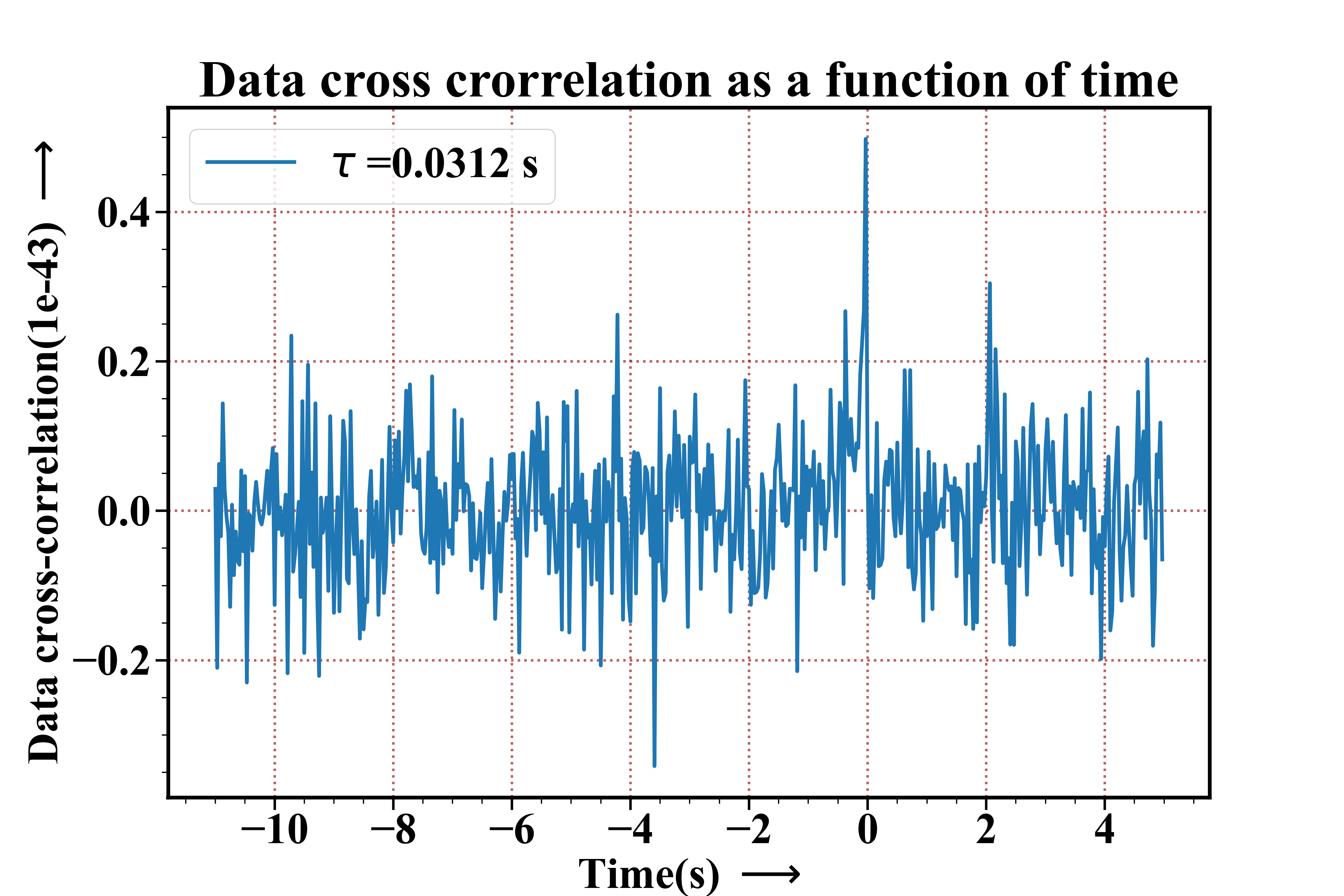
Figure 5: Data containing strongly lensed signal shows a monotonically rising cross-correlation followed by a peak near t=0s. The cross-correlation is performed from the data of a detector at two different times.

In fig. 4 we have shown strongly lensed data for three detectors generated by PYCBC. The lensed signal may contain a constant phase shift in geometric optics that we do not care about (see more in Appendix A), thus we created the lensed signals as $h_{1}^{L}(t)=\sqrt{\mu_{1}}h(t)$ and $h_{2}^{L}(t)=\sqrt{\mu_{2}}h(t)$. The noise is generated from the current PSDs of LIGO and VIRGO detectors. The signal has different strengths in each detector depending upon the antenna pattern of the detector. Thus, the data at any detector $i$ in time-domain

$$d_{i}(t)=s_{i}(t)+n_{i}(t)=F_{\times i}h_{\times}(t)+F_{+i}h_{+}(t)+n_{i}(t),$$ (12)

where $F_{\times i}$ and $F_{+i}$ are the detector antenna patterns of the detector $i$ for the cross and plus polarization respectively. An event with high (or low) SNR between different detectors can give us a good (or bad) sky localization of the source, given the detector antenna function $F_{\times i}$ and $F_{+i}$. Therefore a prior knowledge of the antenna pattern as a function of sky position for a network of multiple (at least two) non-coaligned detectors, we can uniquely determine the best-fit contribution of the strain for both plus and cross-polarization contaminated by the instrument noise. We can use any of these two polarizations for the cross-correlation technique.

When a gravitational wave gets strongly lensed, there can be amplifications of greater than/less than unity, thus the match-filtered SNR of the event may lie above/below the threshold SNR value. The phase shift for strong lensing happens by a constant amount. Therefore the waveform of the signal of the GW gets frequency-independent constant magnification and phase in strong lensing. Then cross-correlating any two GW signals would help us find the similarity between them. Since there is a phase difference of $\pi/2$ between the plus and cross-polarization and each polarization gets an antenna pattern function multiplied, the cross-correlation between the whole strain data containing both polarizations turns out not to be fruitful. Therefore, in practical cases, we cross-correlate between the best-reconstructed contribution on one polarization (say, plus polarization) contaminated by the detector noise. In our simulations, we chose the plus polarization signal of the GW emission and added a Gaussian noise generated from the detector noise PSD. The reconstructed data at a detector $x$ with only one polarization is of the form,

$$d^{p}_{x}(t)=h_{+}(t)+n_{x}(t),$$ (13)

then the cross-correlation between data containing signals in two detectors (given by $d^{p}_{x}$ and $d^{p}_{x^{\prime}}$) can be defined as,

$$D_{xx^{\prime}}(t) =\frac{1}{\tau}\int_{t-\tau/2}^{t+\tau/2}d^{p}_{x}(t^{\prime})d^{p}_{x^{\prime}}(t^{\prime}+t_{d})dt^{\prime},$$

$$=S_{xx^{\prime}}(t)+N_{xx^{\prime}}(t)+P_{xx^{\prime}}(t)+Q_{xx^{\prime}}(t),$$

$$\approx S_{xx^{\prime}}(t)+N_{xx^{\prime}}(t).$$ (14)

The terms on the second expression contains four terms: $h_{+}\times h_{+}$, $n_{1}\times n_{2}$, $h_{+}\times n_{2}$, $n_{1}\times h_{+}$ respectively, where ‘$\times$’ denotes the cross-correlation between them . The cross-correlation is performed over a timescale of $\tau$, with $\tau$ chosen to be a few tens of cycle duration, the cross-terms $P_{xx^{\prime}}$ and $Q_{xx^{\prime}}$ tend towards zero. In this approximation, we are left with only two terms $S_{xx^{\prime}}$ and $N_{xx^{\prime}}$ containing the signals’ cross-correlation and the noises’ cross-correlation .

Fig. 5 shows the cross-correlation performed when the signals are in phase. The signal was injected using PYCBC at $t=0s$ therefore we observe a bump in the cross-correlation near that time. The cross-correlation timescale $\tau$ is varied in accordance with the duration of the time-domain signal, it can be chosen in such a way that it is longer than the typical cycle duration of the GW but much shorter than the whole of the signal duration. The time difference between the data products, $t_{d}$, for a blind lensing search is a free parameter that can be varied from seconds to years. We can define the cross-correlation of data from the same detector but at different times similarly,

$$D_{xx}(t)=\frac{1}{\tau}\int_{t-\tau/2}^{t+\tau/2}d^{p}_{x}(t^{\prime})d^{p}_{x}(t^{\prime}+t_{d})dt^{\prime}\approx S_{xx}(t)+N_{xx}(t).$$ (15)

Fig. 6 shows the cross-correlation of noise at two different times when the signal is not present. The random noise fluctuations have a mean of zero and thus taking the cross-correlation of two noise entities for a long enough timescale, always tend it towards zero. In fig. 7 we show the cross-correlation between the data containing GW signals for strong lensing. The signal has its max amplitude at t=0, set here, thus we can observe a gradual rise in the cross-correlation signal followed by a peak around t=0s and with a sharp fall the pattern disappears and is again dominated by noise fluctuations. Thus if we cross-correlate two time-series data containing the same GW event in phase, we expect to observe a positive monotonically increasing cross-correlation as the chirp continues, followed by a sharp drop after the instance of the BBH merger. In appendix A, we have shown a few tests to show the robustness of this technique in distinguishing signal from noise.

Sometimes, there can be persistent noise sources near a detector site, in that case, we cannot take the data chunks from one detector and cross-correlate with another data chunk from the same detector with a certain time difference. This is required to avoid dominance by the $N_{xx^{\prime}}$ term over the $S_{xx^{\prime}}$ term. For correlated noise, we have to pick the data from two detectors at different locations to cross-correlate. We claim that a blind search in all available LVK data has to be performed in search of lensed GW signals using this technique. For strong lensing, the obvious choice to try something first would be cross-correlating data from one detector at different times.

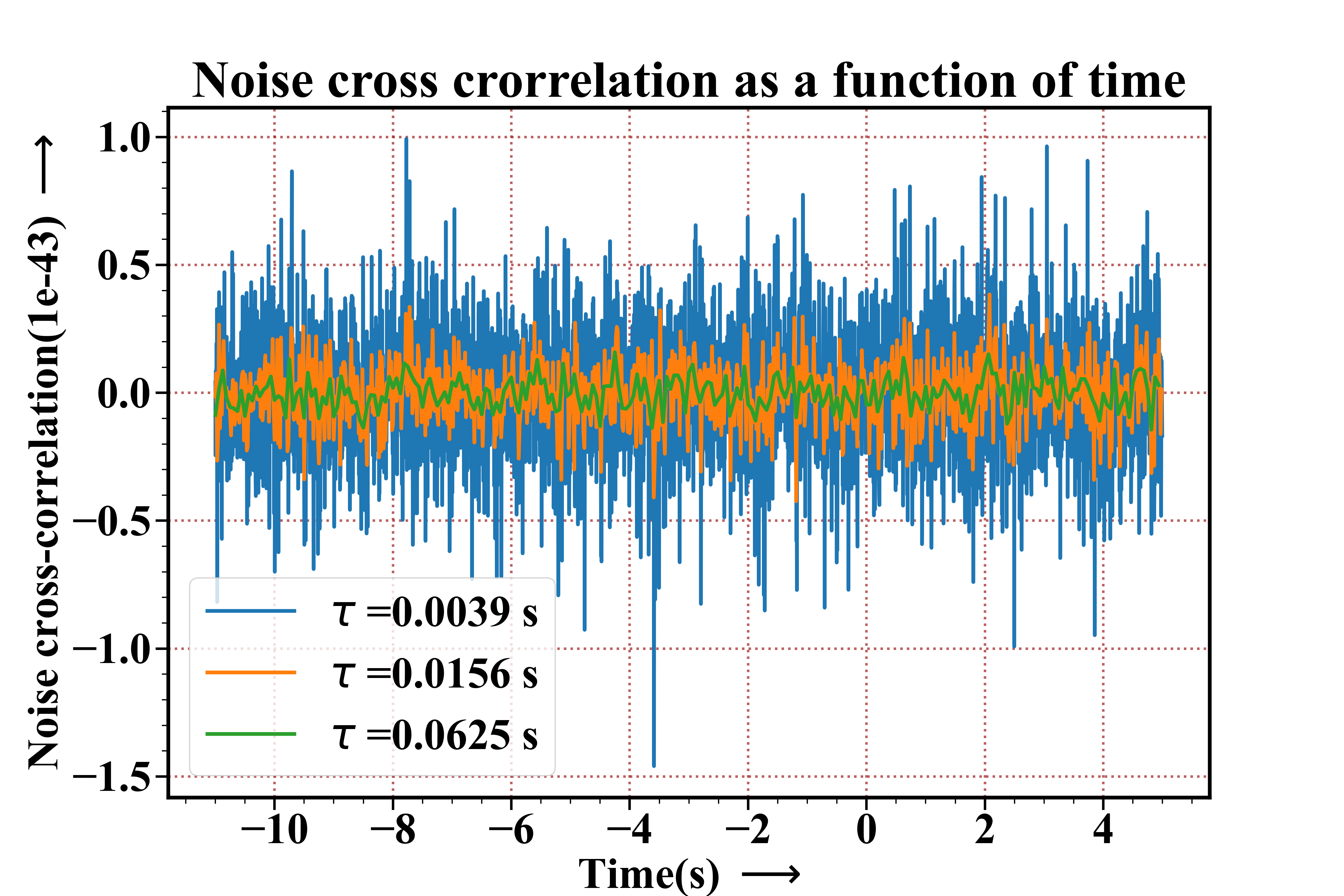
Figure 6: Noise cross-correlation at different times, shows random variation about mean cross-correlation of zero. The fluctuations go down with increasing cross-correlation timescale.

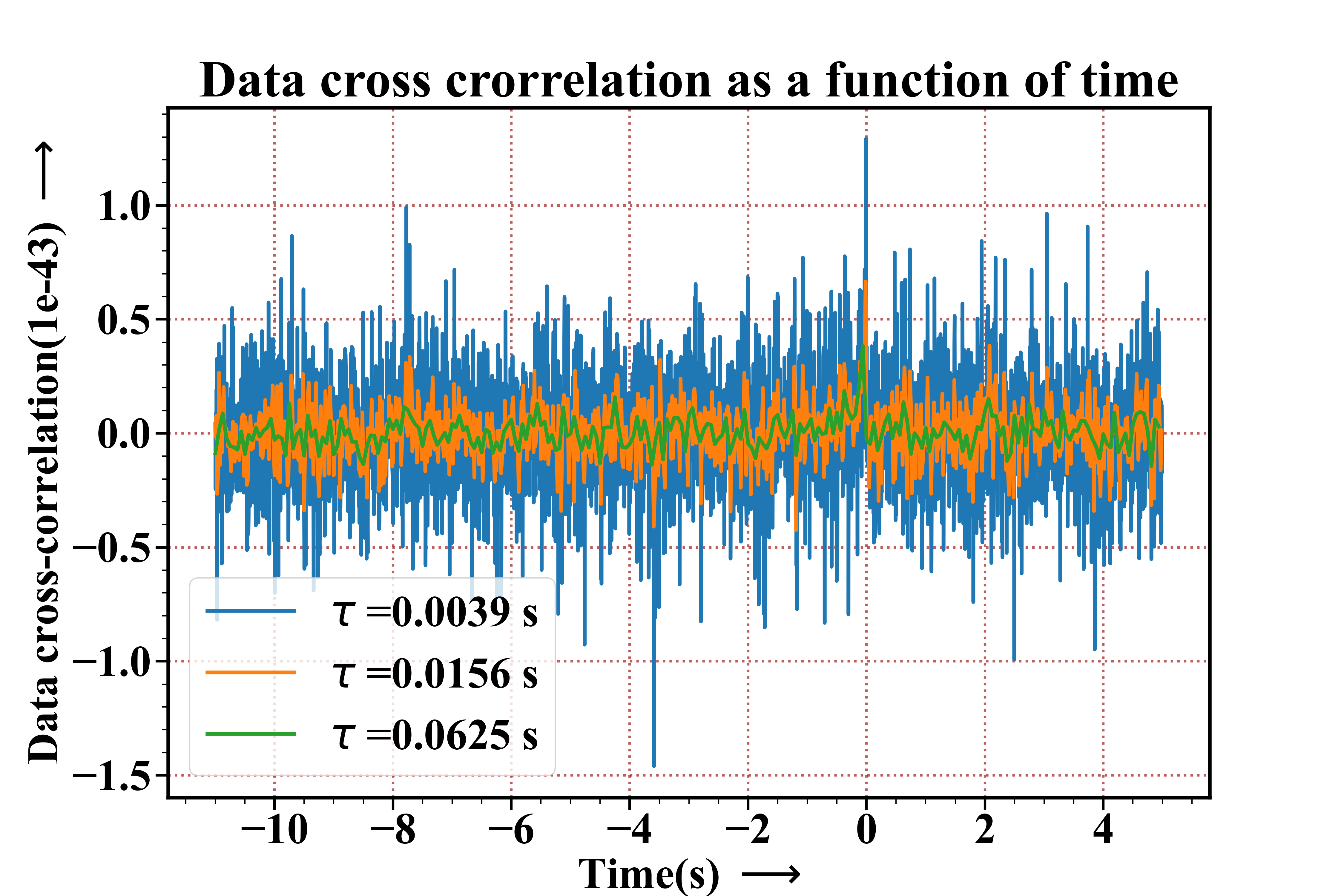
Figure 7: Variation of the strongly lensed cross-correlation signal with cross-correlation timescale. With increasing cross-correlation timescale, the noise fluctuations go down making the signal cross-correlation more prominent.

To generalize, if $n$ images are created by strong lensing, then with a network of $m$ detectors, we can have at most $\frac{mn(mn-1)}{2}$ number of cross-correlations . However, $n\frac{m(m-1)}{2}$ of these are the cross-correlations between the almost simultaneous events, and thus do not bear significant importance in the lensing analysis.

5.2 Confirmation of detection of a lensed signal

We observed the cross-correlation signal when a signal is present, but confirmation of lensing requires mitigating the noise as much as possible. To qualify an event as a lensing candidate, we take the binned average of these data cross-correlations $\langle D_{xx^{\prime}}(t)\rangle$ and calculate how much it deviates from typical averaged noise cross-correlation $\langle N_{xx^{\prime}}(t)\rangle$. The noise cross-correlation ($N_{xx^{\prime}}$) is obtained when no signal is present. The deviation of the averaged data cross-correlation from the averaged noise cross-correlation helps us calculate an effective lensing signal-to-noise ratio or SNR ($\rho$) from the cross-correlations. We define the square of SNR for the lensing cross-correlation as :

$$\rho^{2}(t)=\left(\frac{\langle D_{xx^{\prime}}(t)\rangle-\langle N_{xx^{\prime}}(t)\rangle}{\sigma_{N}(t)}\right)^{2}.$$ (16)

Given the timescale $\tau_{snr}$ corresponding to n points of data cross-correlation, the average is taken as, $\langle D_{xx^{\prime}}(t)\rangle=\dfrac{\sum_{i=1}^{n}D_{xx^{\prime}}|_{i}}{n}$ implying $D_{xx^{\prime}}|_{i=1}=D_{xx^{\prime}}(t-\tau_{snr}/2)$ and $D_{xx^{\prime}}|_{i=n}=D_{xx^{\prime}}(t+\tau_{snr}/2)$ and same goes for $\langle N_{xx^{\prime}}\rangle$,

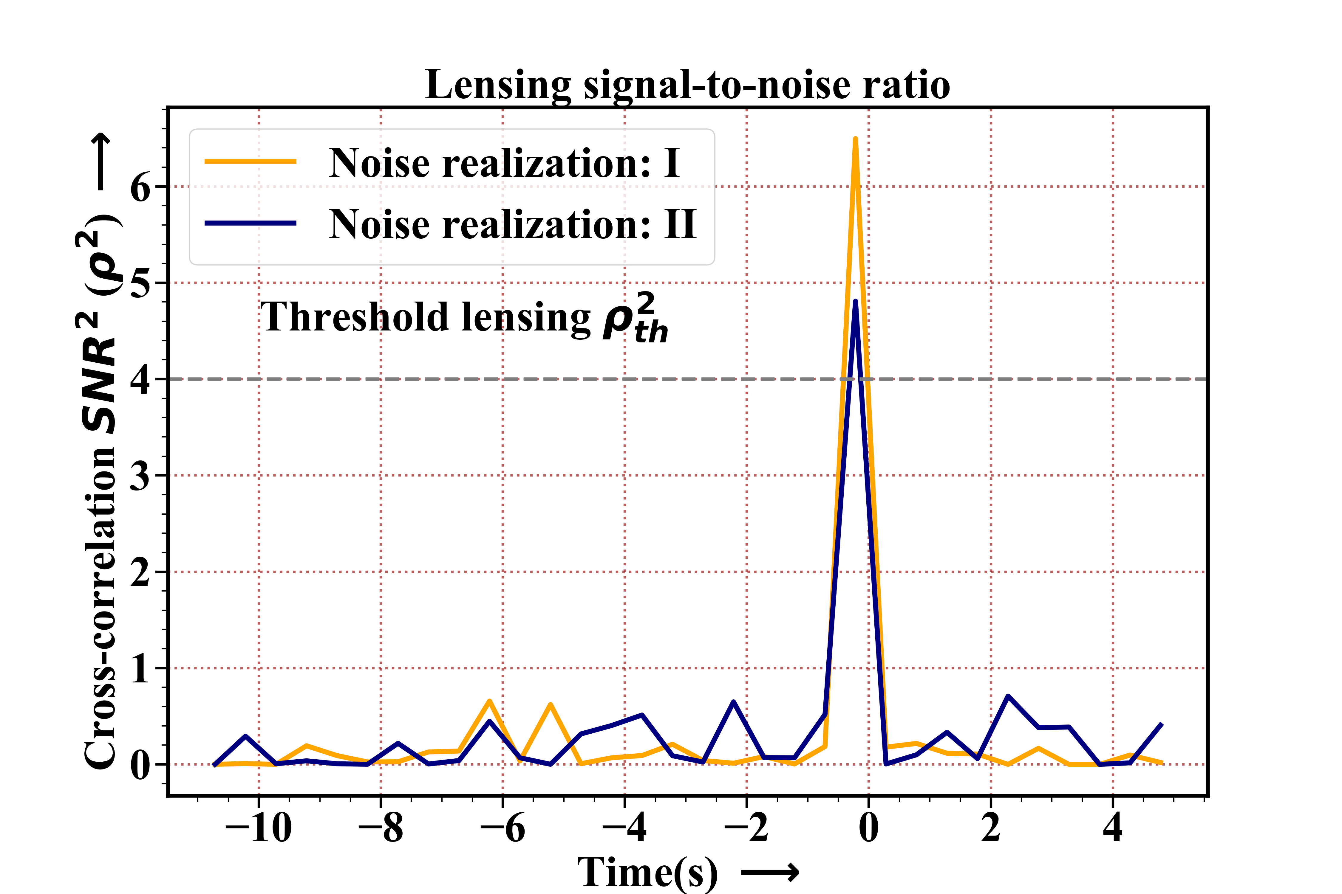
Figure 8: Lensing signal-to-noise ratio for the strong lensing case, with $\tau_{snr}=0.5s$. It depicts the typical deviation of the data cross-correlation from the noise cross-correlation. We can set a threshold lensing SNR, which informs us about the significance of the event being lensed.

where $D_{xx^{\prime}}$ and $N_{xx^{\prime}}$ are defined in equation 5.1; $\sigma_{N}$ is the standard deviation of $N_{xx^{\prime}}$ for the given bin. Averaging of $D_{xx^{\prime}}$ and $N_{xx^{\prime}}$ is done over a timescale of $\tau_{snr}$ around any particular time $t$, this is known as the binned average. Note that, this definition of $\rho^{2}$ is quite different from the match-filtering SNR. We confirm the lensing of the signal by calculating the lensing SNR of the event(s). The total lensing SNR for the event is obtained by adding lensing SNRs from different data channels in quadrature. The events with total $\rho^{2}_{\rm event}>\rho^{2}_{th}$ can be qualified as lensing detection given their sky positions match significantly.

Fig. 8 shows the time variation of the lensing SNR for two different noise realizations. There is a significant jump in the SNR around $t=0s$ caused by the presence of the signal. The threshold value of $\rho^{2}$ above which we call a lensing candidate can be calibrated by observing the typical SNR of noise cross-correlation. Although both of the noise realizations have several spikes, the tallest peak is obtained at the time of signal injection. Judging by the typical SNR of noise cross-correlation for these two scenarios (which shows a significant drop in the lensing SNR for bad noise realizations) we can choose this threshold to be at $\rho^{2}_{th}=4$ for the case with $\tau_{cc}=0.03125s$ and $\tau_{snr}=0.5s$. The timescale of SNR can be made as large as the duration of the signal, for maximum suppression of the noise fluctuations. Even then, there can be peaks in the SNR of the same order/higher than the signal SNR when there is a strong noise source in some detector(s). The validation of the signal (and distinguishing it from the noise) can be possible from multiple cross-correlation signals between different pairs of detectors. All the data chunks which show a common cross-correlation between different pairs of detectors, can be explored based on the strain data using both amplitude and phase and estimating the source parameters of the sources. We have shown the impact of different noise realizations on the cross-correlation method in appendix C.

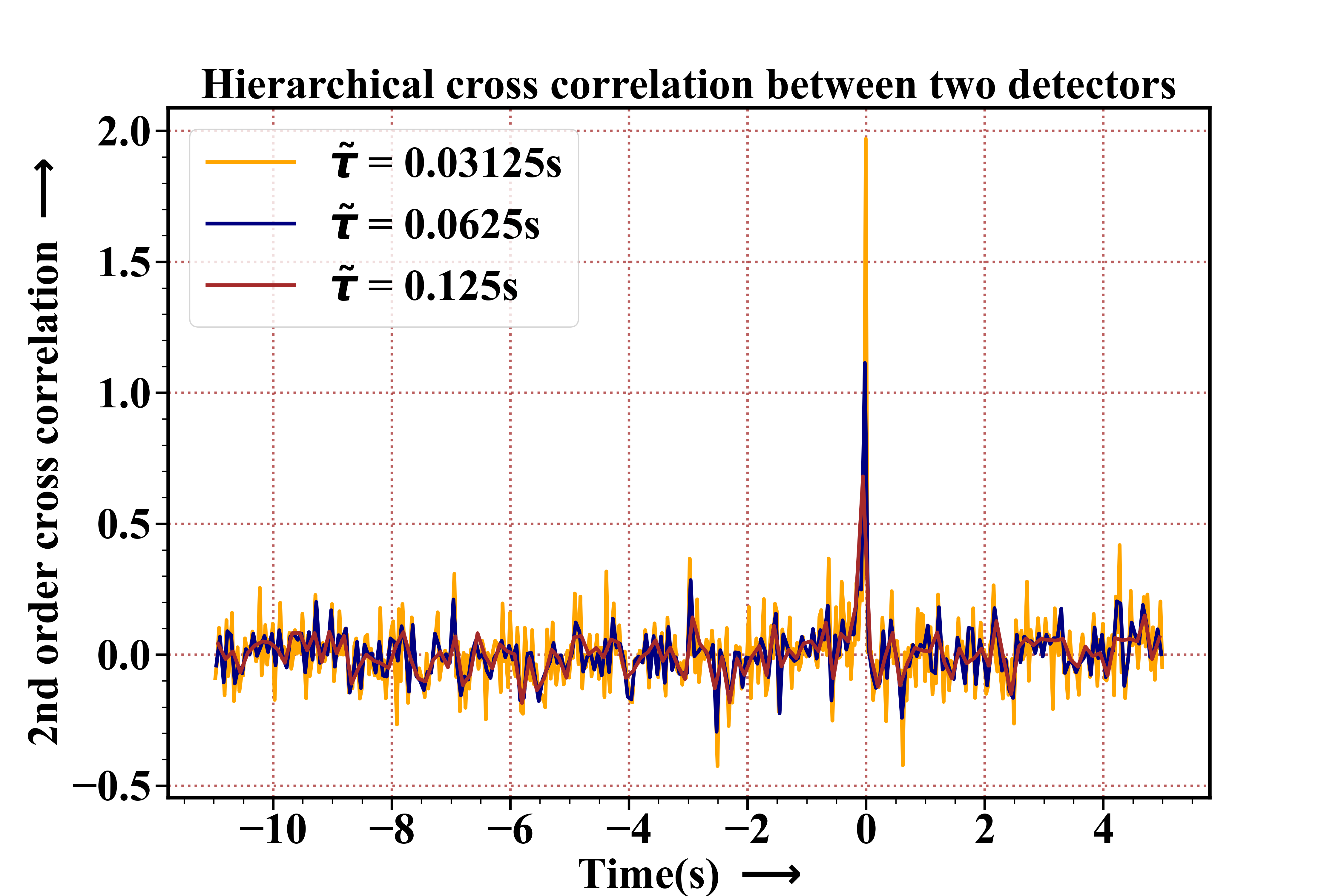
Figure 9: Hierarchical cross-correlation conducted between cross-correlation signals from two different detectors. The noise is further suppressed than the cross-correlation. However, any two monotonically increasing positive noisy functions can, in principle, produce a similar pattern. This is because the phase information of the signal is not relevant here. This makes it a little sloppy for the detection of lensed signals.

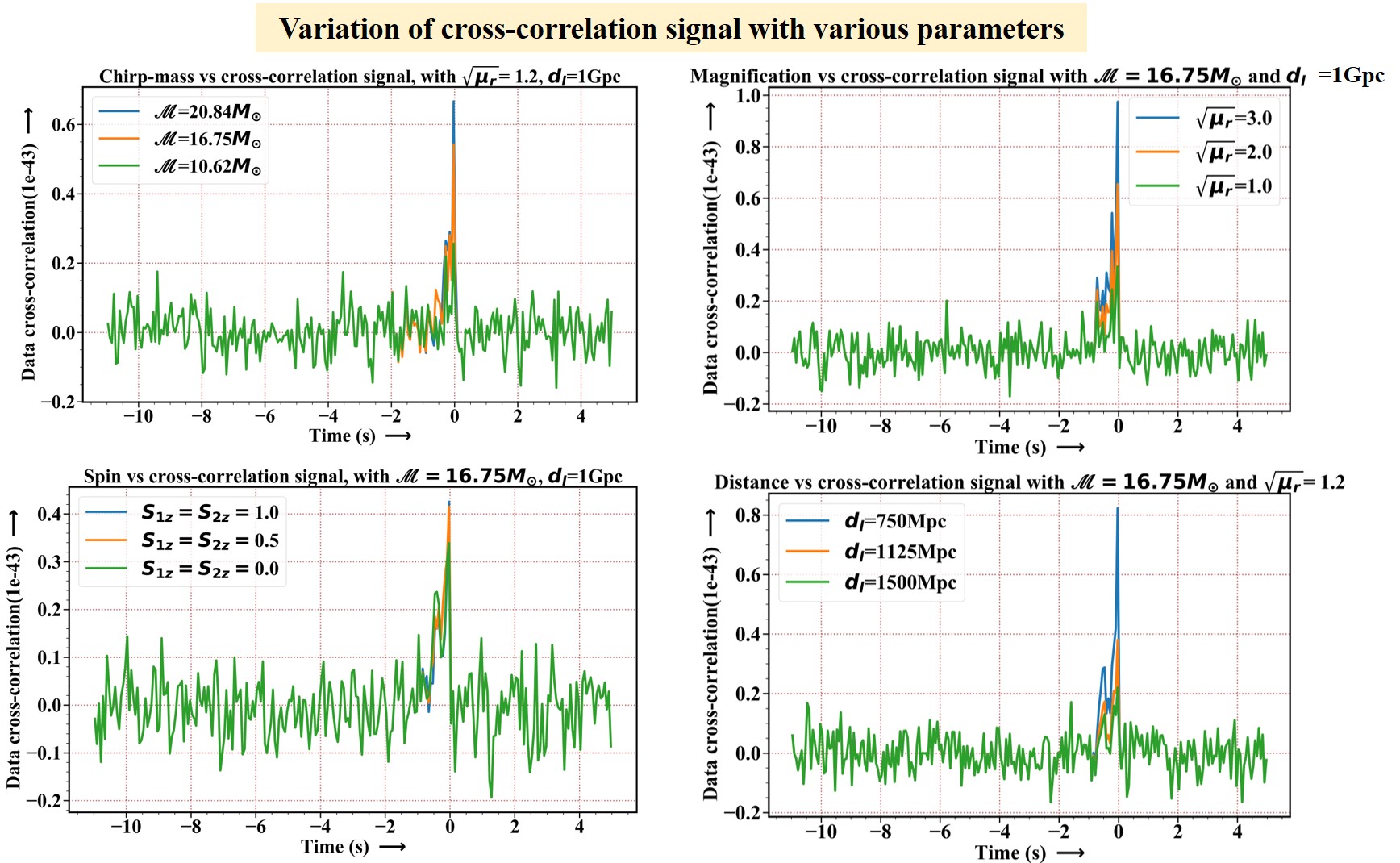
Figure 10: Variation of the cross-correlation signal with respect to the source parameters (chirp mass of the source, its luminosity distance, and the spin components along its orbital angular momentum) and lens-induced parameters (magnification). The timescale of the cross-correlation is chosen to be $\tau=0.0625s$.

In the hope of further improving the lensing detection significance, we used hierarchical cross-correlation performed on the data cross-correlation $D_{xx^{\prime}}$ between different two different pairs of detectors. The second-order cross-correlation takes the cross-correlation of the data and cross-correlates it again; it is defined as,

$$\Delta_{xx^{\prime}}(t)=\frac{1}{\tilde{\tau}}\int_{t-\tilde{\tau}/2}^{t+\tilde{\tau}/2}D_{xx}(t^{\prime})D_{x^{\prime}x^{\prime}}(t^{\prime}+T_{d})dt^{\prime},$$ (17)

where $\tilde{\tau}$ is the cross-correlation timescale here and $T_{d}$ is the time-shift required for the cross-correlation signals to overlap. In fig. 9 we can observe that the 2nd-order signal cross-correlation is more prominent than the 1st-order cross-correlation signal taken between the raw data itself. Noise fluctuations are suppressed with increasing $\tilde{\tau}$. However, this cross-correlation does not incorporate the phase of individual signals, two gradually rising patterns of positive values arising from any source, whether be it astrophysical or terrestrial in origin, would produce a 2nd order signal cross-correlation like this. Higher-order cross-correlation works better if the signal duration is pronounced for very long (minutes-long GW signals, so that finding a pattern for the cross-correlation is easier) durations, but for short signals(of the order of seconds), such higher-order correlations are not reliable in terms of searching for lensed signals. Thus, to avoid triggers that are generated from two distinctly different sources with similar source parameters (or from some strong and short noise source), we would emphasize doing the cross-correlation on phase and we abstain from using hierarchical cross-correlation here in this analysis.

5.3 Dependency of Cross-correlation signal on source and lens parameters

It is necessary to check the source parameter dependency of the signal cross-correlation to understand the possible range of parameter space that can explored using the cross-correlation method. Thus in fig. 10, we have shown the dependency of the cross-correlation signal on different source parameters as well as lens modification, i.e. magnification, and observe the signal cross-correlation strength as compared to noise cross-correlation. The first of the plots shows the variation of the signal cross-correlation with the chirp mass. As can be seen, the method can work well for sources with chirp mass as low as 10 M_⊙ at 1Gpc. As we have increased the chirp mass of the source, individual signals get stronger resulting in a higher peak value in the cross-correlation. The next plot shows the variation of the same with respect to the relative magnification. Relative magnification is the boost in the signal because of the presence of the lens. As relative magnification goes up, signals have a greater contribution to data in comparison to noise, so the signal cross-correlation peak goes up with increasing magnification. The next plot shows the variation of the cross-correlation signal keeping the chirp mass fixed at 12.16 $M_{\odot}$, we varied the luminosity distance of the source. Increasing the luminosity distance makes the signal fainter, thus with increasing distance peak height goes down. As can be seen, up to a luminosity distance of $1$ Gpc with a magnification factor of $\sqrt{\mu_{r}}=1.2$, it performs well. As seen here, relative magnification and luminosity distance are two counter-acting quantities on the signal. As we will later see, there lies a degeneracy while estimating these two parameters, which is resolved in a later section. The dependency of the signal cross-correlation strength with respect to the spins (along the orbital momentum, i.e. z-direction) of the source BBH is not very conclusive.

In fig. 8, we found how the lensing SNR ($\rho$) varies with time as the signal passes through the detectors. We added the values of $\rho^{2}$ to find the total $\rho^{2}$. We took a fixed set of source parameters and magnification to create our data-I and fixed all other parameters except one to create the data-II. Then we varied that single parameter and checked how the lensing SNR varies as the variable parameter approaches the data-I injection parameter. Variation of the total $\rho^{2}$ provides us with an idea about the source parameters that are degenerate with the lens parameters. We show the variations of the total of squared SNR vs different parameters in fig. 11. As we approach the data-I injected parameter by varying data-II variable parameter, we observe a sharp peak which diminishes away from that injection value. This shows that, although a background of total $\rho^{2}$ is present for all these cases, it only peaks when we are significantly close to the injection. The plots also show that, as we increase the SNR timescale $\tau_{snr}$, in most of the cases the recovery of the injected data-I chirp mass and spins is successful, as the most dominant peak is present at that very position. Only with certain unfavourable noise realizations and bad choice of timescales ($\tau_{snr}$ should be at least 20 times longer than the cross-correlation timescale, now called as $\tau_{cc}$ to avoid any confusion) led to the inability of the recovery as shown in the mass and spin pane of fig. 11 for $\tau_{cc}=0.016s$ and $\tau_{snr}=0.125s$. Another way to quantify the SNR of the signal is to use the maximum SNR at the time when the cross-correlation signal peaks, instead of the integrated SNR at all times around the signal. The performance of our method using max SNR is shown in appendix D.

However, the variation of the total $\rho^{2}$ with respect to relative magnification or luminosity distance is rather monotonic and it does not show any peak in the SNR. Therefore, one can easily understand that the signal contains degeneracy in overall magnification and luminosity distance since a proper combination of those values can help to completely reconstruct the data-I signal starting from the data-II signal. Thus we need to apply parameter estimation techniques to find the range of values these source and lens parameters can take. We will discuss this thoroughly in the coming section.

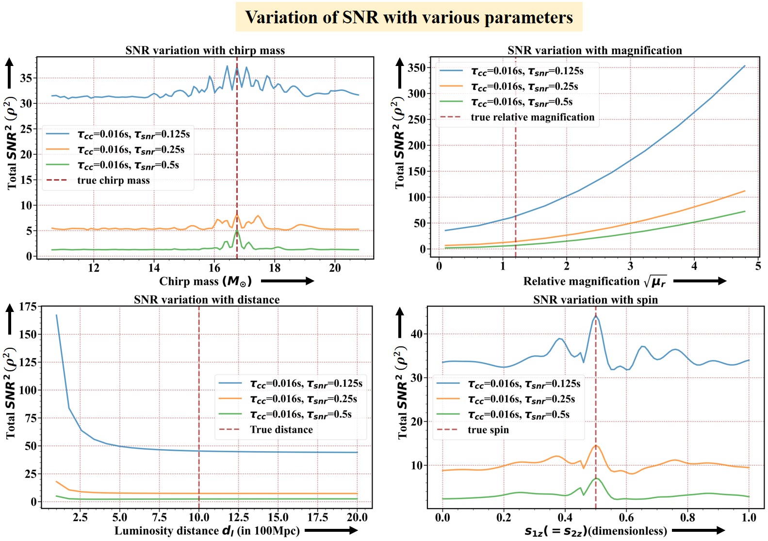
Figure 11: Variation of the lensing SNR with chirp mass, relative magnification, luminosity distance, and spins. It shows that the injection of the parameters is successful for chirp masses and spins, but not for luminosity distance and relative magnification.

6 Lens and GW source characterization based on cross-correlation signal

Since gravitational lensing substantially changes the waveform of gravitational waves, inference of source parameters with no lensing produces significantly different results than inference of them with lensing. Some source parameters with no lensing are degenerate with some other source parameters with the lensing hypothesis. This makes the parameter estimation extremely challenging. For strong lensing cases, when the signal is amplified by a constant factor thus, only luminosity distance $(d_{l})$ and relative magnification factor $(\sqrt{\mu_{r}})$ are such degenerate parameters. Because strain is proportional to $1/d_{l}$ and if lensed it is proportional to $\sqrt{\mu}$ if lensing is not considered, we would infer the luminosity distance to be $d_{l}/\sqrt{\mu}$, making that a completely different event by itself. However, for two data strains, we cannot estimate three degenerate parameters ($\sqrt{\mu_{1}}$ and $\sqrt{\mu_{2}}$: the magnification of each signal and $d_{l}$: the true luminosity distance of the source) from it. Thus the reduced form of the two individual magnifications $\sqrt{\mu_{r}}$ along with the luminosity distance $d_{l}$ are the two parameters that can be estimated. This is shown in fig. 12. We took a merging BBH as a GW source; the component masses are $15M_{\odot}$ and $25M_{\odot}$ at a distance of 1Gpc and one signal had a relative magnification of $1.5$ with respect to the other. When we infer their luminosity distance considering no lensing, one inference of $d_{l}$ falls in place but the magnified one shows a smaller $d_{l}$ inferred. However, with lensing, we are getting the correct luminosity distance as well as the relative magnification. Different component masses substantially change the signal duration and its frequency-chirping, spins can too alter the waveform significantly. Thus these parameters do not fall into the category of degenerate parameters. Thus we currently restrict our estimation to two parameters. However, for microlensing cases masses and spins parameters can be degenerate with the lens-invoked parameters, which we are working on for future work to explore the joint parameter space of the source and the lens (Chakraborty & Mukherjee, 2024a).

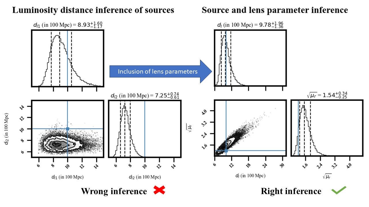
Figure 12: The parameter space for no lensing hypothesis is different from that considering lensing to occur. Without the strong lensing hypothesis, there is no existence of lensing magnification which plays a role in inferring the true luminosity distance of the source. It shows that, if two strongly lensed images have a relative magnification of $\sqrt{\mu_{r}}=1.5$ with sources at $d_{l}=1$Gpc, we get a wrong inference of individual luminosity distance of the two events. Thus the inclusion of lens parameters along with the source parameters jointly is necessary for parameter estimation of the events.

We have used Bayesian analysis to estimate the source parameters and lens modulations on the lensed GW signal. The Bayes’ theorem is given by,

$$p(\vec{\theta}|d)\propto L(d|\vec{\theta})\Pi(\vec{\theta}),$$ (18)

where $\Pi(\vec{\theta})$ is the prior on the luminosity distance and relative magnification, provides the prior information known about the different source and lens parameters, $L(d|\vec{\theta})$ is the likelihood, describing the probability of obtaining the data with the chosen prior for different parameters and $p(\vec{\theta}|d)$ is known as the posterior. There is an overall normalization factor, $p(d)$ known as the evidence.

The data at any detector $\textnormal{d}_{i}=F_{\times i}h_{\times}+F_{+i}h_{+}+n_{i}$ is given in terms of the unlensed model is given by,

$$\textnormal{h}^{ul}_{i}=F_{\times i}h^{ul}_{\times}(\vec{\theta})+F_{+i}h^{ul}_{+}(\vec{\theta})\quad.$$ (19)

By choosing a flat prior for the parameters and a Gaussian likelihood, we also expect to get a Gaussian posterior. The choice of the likelihood for cross-correlating two different time-domain data is mentioned below:

$$-\log(L)=\frac{(d_{1}-h^{m}_{1})^{2}}{2\sigma_{n1}^{2}}+\frac{\log(2\pi\sigma_{n1}^{2})}{2}+\frac{(d_{2}-h^{m}_{2})^{2}}{2\sigma_{n2}^{2}}+\frac{\log(2\pi\sigma_{n2}^{2})}{2}.$$ (20)

$d_{1}$ and $d_{2}$ are the data chunks that pass through all aforesaid tests, $\sigma_{n1}$ and $\sigma_{n2}$ are the noise standard deviation associated with them in the absence of any signal.

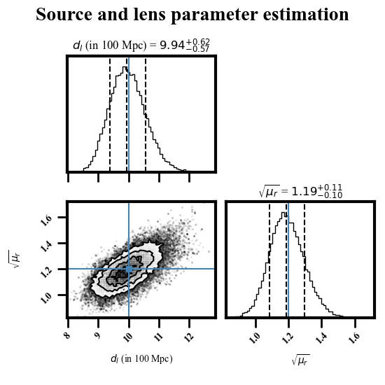
Figure 13: Strong lensing parameter estimation: We ran Markov-chain Monte-Carlo sampling for simulated lensed GW signals with BBH component masses of $m_{1}=15M_{\odot}$ and $m_{2}=25M_{\odot}$ with luminosity distance $d_{l}=1Gpc$ and a relative magnification of $\sqrt{\mu_{r}}=1.2$. The injected parameters luminosity distance ($d_{l}$) and relative magnification ($\sqrt{\mu_{r}}$) are well recovered in our inference of the 2D joint source and lens parameter space.

Model for strong lensing: $h^{m}_{1}=\sqrt{\mu_{r}}h_{1}^{ul}(d_{l})$ for the higher SNR signal and $h^{m}_{2}=h_{2}^{ul}(d_{l})$ for the lower SNR signal and $d_{l}$ and $\sqrt{\mu_{r}}$ are the parameters to estimate. The prior for luminosity distance is chosen to be: $d_{l}\in[100\rm{Mpc},5\rm{Gpc}]$ and for relative magnification it is: $\sqrt{\mu_{r}}\in[0.1,10]$ . The model consists of all the parameters of interest. After the posterior is obtained, we employ a Markov Chain Monte Carlo sampler using the python-module emcee to obtain the posterior distribution of the parameters. For strong lensing, the results are shown below in fig. 13, the blue lines show the injected values of the parameters. We can see the injected values of the parameters (shown by blue solid lines) lying inside the 95% confidence interval around the median. The application of this technique for more than two lensed events is discussed in appendix B.

We tested our method on a range of cases with varying chirp mass of the BBH and checked the consistency that this method provides. The other parameters being fixed, the chirp mass itself decides the match filtering SNR of the event. Thus we have shown the variation of how well our parameter estimation works over a range of match-filtered SNRs of the louder event. The violin plot in fig 14 shows the inference of the luminosity distance with the increasing match-filtered SNR. The match-filtered SNR is a proxy to the strength of the signal, thus with increasing SNR, the parameter estimation goes closer to the injection value for the luminosity distance. Similarly, in fig. 15 we show the parameter estimation performs on relative magnification inference. The match-filtered SNR increase again points towards a better inference of the injection value of the $\sqrt{\mu_{r}}$. These runs essentially test the robustness of the whole framework, before we start trial runs on the available LVK data looking for traces of lensing signature in the strong lensing regime using GLANCE.

To summarize, we applied a cross-correlation technique to detect lensed gravitational waves. We claim that to search for lensed GW signals, a blind search on the LVK time-series data (both below and above threshold ) from different/same detectors has to be performed. Cross-correlation provides us with an insight into the degree to which two noisy signals are similar. We have calculated the lensing SNR ($\rho$) given the data cross-correlation to qualify an event as lensed. For lensing $\rho>\rho_{th}$, we called it a lensing candidate. For such candidate events, we have used joint parameter estimation techniques to extract relevant source parameters degenerate with the lens signatures on the GW waveform.

7 Conclusion

We developed a new technique called GLANCE to find lensed gravitational wave signals. It relies on the fact that two data pieces contain GW signals with very similar characteristics, such that their overlap is a non-zero quantity over a certain time . The data can be from one detector at multiple times or multiple detectors at the nearly same time, and cross-correlating such data with un-correlated noise picks up the signal while suppressing noise. The cross-correlation between different detectors showing a monotonic rise followed trend affirms the presence of two similar GW signals. We estimate the lensing SNR of the cross-correlation to qualify an event as a lensed candidate if the lensing SNR is above some threshold. Estimation of GW source parameters and lens parameters are performed on those candidates’ cases. It has been found that for above threshold ($>\rho_{th}$) SNR signals, the parameter estimation can extract the source and lens properties, and simulation results agree well with the injected values for those cases.

To mention a few salient features of this technique, firstly, it can work well even in the sub-threshold regime. We obtained that when the match-filtered SNR of the event is low, we can explore the degeneracies in the parameter space but with some compromise in the precision of the results. . Secondly, this technique can combine data from multiple detectors and mitigate the uncorrelated detector noise. It can join the searches in the sub-threshold level along with the currently existing pipelines (McIsaac et al., 2020; Li et al., 2023).Thus even if a detector misses to observe a sub-threshold event, we can use other detectors to get the lensing search continued. And finally, but not the least important, this technique does not depend on any particular model of lensing. It can search for any kind of lensed GW signal through cross-correlation between data pieces.

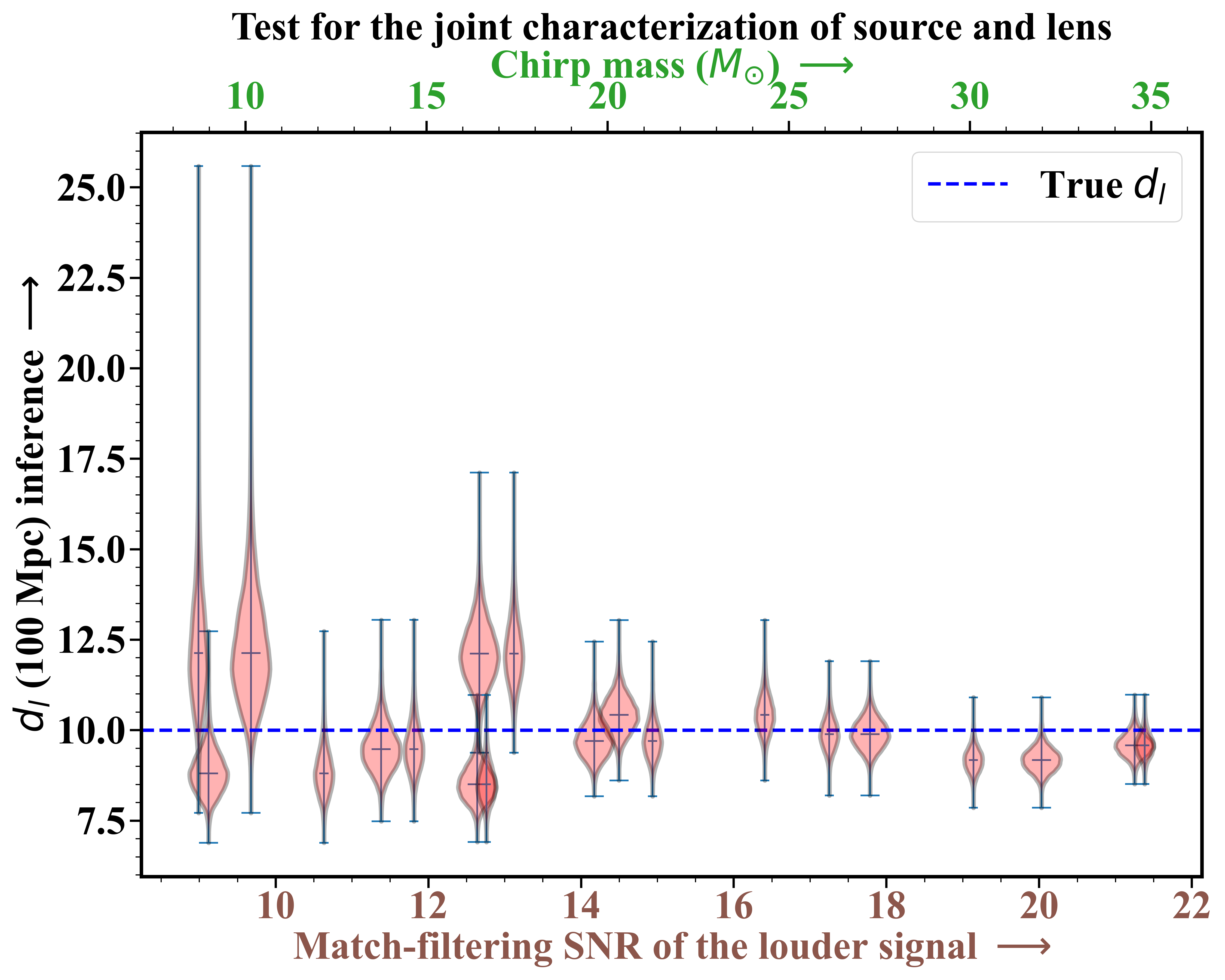
Figure 14: Luminosity distance inference for a range of chirp mass which then is translated in terms of match-filtered SNR since all other parameters are kept fixed. Thus we have shown how the parameter estimation for $d_{l}$ works while varying the strength of the signal. Thus we have both chirp mass and match-filtered SNR along the x-axis. The figure shows that with increasing match-filtered SNR of the louder signal (which has a relative magnification of 1.2 with respect to the fainter one), the estimation of $d_{l}$ gets better, and we obtain a narrower posterior.

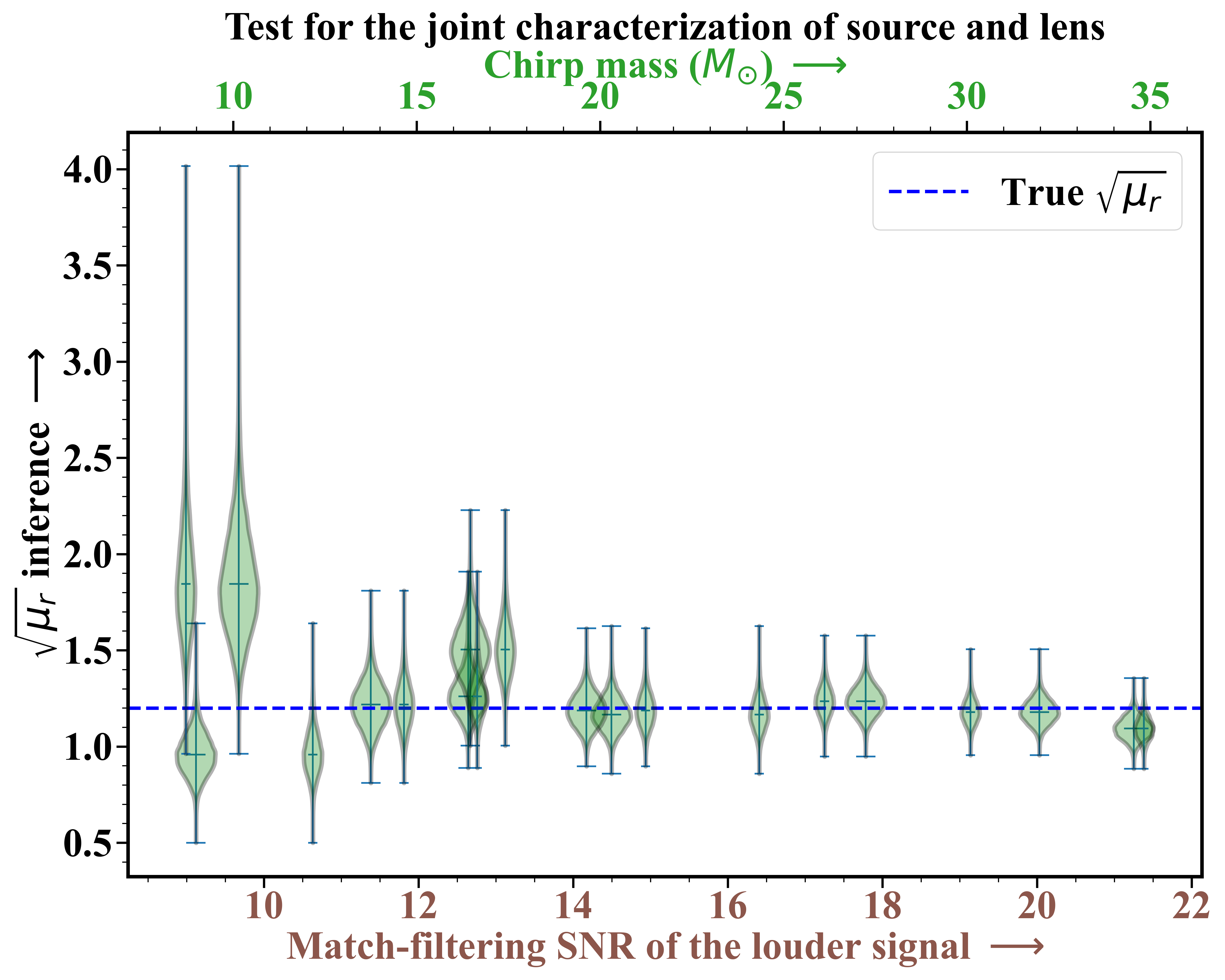
Figure 15: Relative magnification inference for a range of chirp mass (as well as the match-filtered SNR of the louder event). The posterior distribution of the parameter is narrower around the injection value as the math-filtered SNR of the brighter source is increased.

One of the key aspects is to understand the false alarm rate for the detection of the lensed events. False alarms can be there when different events of similar source properties lie close in the sky-localization. Since the GW source localization is currently not that good, false alarms can become a menace to deal with (Çalışkan et al., 2023b). However, The sky position of the GW source will improve drastically after LIGO-Aundha(India) becomes online (Shukla et al., 2023). With more and more detectors online like Cosmic Explorer (Hall, 2022), Einstein Telescope (Punturo et al., 2010) or LISA (Çalışkan et al., 2023a), this GW localization challenge will gradually fade away (Pankow et al., 2018). However, within our accuracy of source localization, there can be actually two BBH-merger events with the same source parameters, giving rise to a false lensing alarm. To resolve this, population studies of black holes as well as merger rates at different redshifts have to be considered. We will explore this in a future work, that is currently under preparation (Chakraborty & Mukherjee, 2024b).

In summary, this new technique GLANCE is capable of detecting lensed GW events from the noisy data for both sub-threshold and well-detected events. The application of this technique to the GW data makes it possible to detect lensed events with high confidence and characterize the lens and source properties. In reality, we don’t have any idea whether a signal is strongly lensed or microlensed until its source and lens parameters are completely understood. Thus in the future, this work will be extended to the micro-lensing searches using GLANCE (Chakraborty & Mukherjee, 2024a) to explore a a higher dimension of source parameter space degenerate the lens-imposed ones. . With the moderate number of GW events detectable from current-generation and next-generation GW detectors, the application of this technique will make it possible for robust detection of lensed GW signals.

Data Availability

The simulation scripts will be available in the ⟨data|theory⟩ Universe-Lab Github site. Its usage in a research work must be done with proper consent from the authors.

Appendix A Off-phase cross-correlation of two signals and noise cross-correlation with signal: Two essential tests for the GLANCE framework

We have observed the cross-correlation of noise with itself (at two different instants) in fig. 6 and the cross-correlation of a signal with itself in fig. 5. However, one may wish to explore how the signal cross-correlated with noise appears. Keeping this in mind, we have shown the same in fig. 16.

As can be seen here, we cannot distinguish any pattern in the signal unlike fig. 6. We are safe to say that, noise cross-correlated with data with signal does not show any cross-correlation pattern. Therefore, such cases won’t pose a threat to this technique generally. However, the presence of persistent terrestrial noise sources would require us to higher the lensing SNR threshold $(\rho_{th})$.

While, writing eq. 5.1, we essentially assumed that we have already found two signals separated by a time delay of $t_{d}=t_{d0}$. However, as we mentioned there, in practical cases we are running a blind search for other signals, making $t_{d}$ a free parameter. In some cases, when the signals have some overlap but not lying exactly on top of one another, we can have a mild-cross-correlation signal. To check, whether we would receive a strong signal cross-correlation, we have plotted the cross-correlation of two signals in fig. 17. Here the peaks of the two signals are separated by 0.244s, with signals each having a duration of about 1s . We can observe that this off-phase cross-correlation appears similar to the noise cross-correlation in fig. 6, whereas the on-phase cross-correlation (with signals’ peaks lying on top of each other) shows a monotonically increasing trend and then a sharp fall. Additionally, we have shown in fig. 18 that while cross-correlating between two pieces of data, how the cross-correlation signal varies for each polarization with respect to the phase-shift due to lensing. If we take the cross-polarization piece from the data and cross-correlate it with the two polarizations of another data, the signal strengths are quite complementary when plotted against phase-shift. Here the domain for the phase-shift is chosen to be $\theta=[0,\pi]$. The cross-polarization signal strength monotonically goes down with increasing phase difference, crossing zero and going to negative values near the phase difference of $\pi/2$. The plus polarization cross-correlation first increases with a phase difference, becomes maximum at $\pi/2$, and then goes down. This shows that if there is a phase shift of $\pi/2$ in the $h_{+}$ (or $h_{\times}$) GW signal due to lensing, then $h_{\times}$ (or $h_{+}$) polarization can be used to recover it. These three tests are a must to check the consistency of the whole mathematical framework. Our tests show that the technique passes well through these tests. Thus when this technique shows a nice rising trend followed by a peak, we check the origin of this signal cross-correlation, by evaluating its SNR and running a parameter estimation with those two data-pieces.

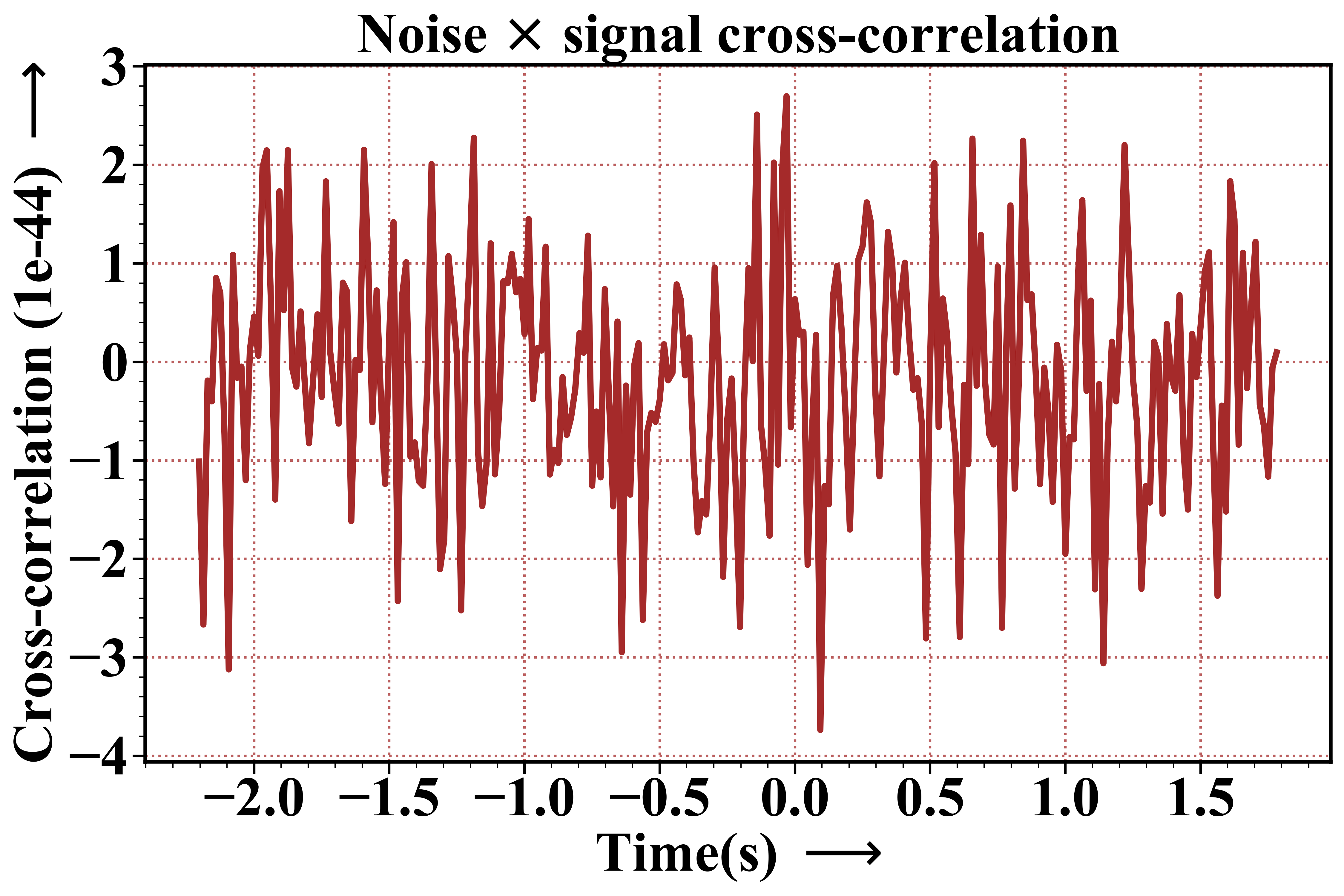
Figure 16: Cross-correlation between noise and signal shows no evidence of a trend similar to signal cross-correlation. Here the cross-correlation timescale is chosen to be $\tau_{cc}=0.0625s$.

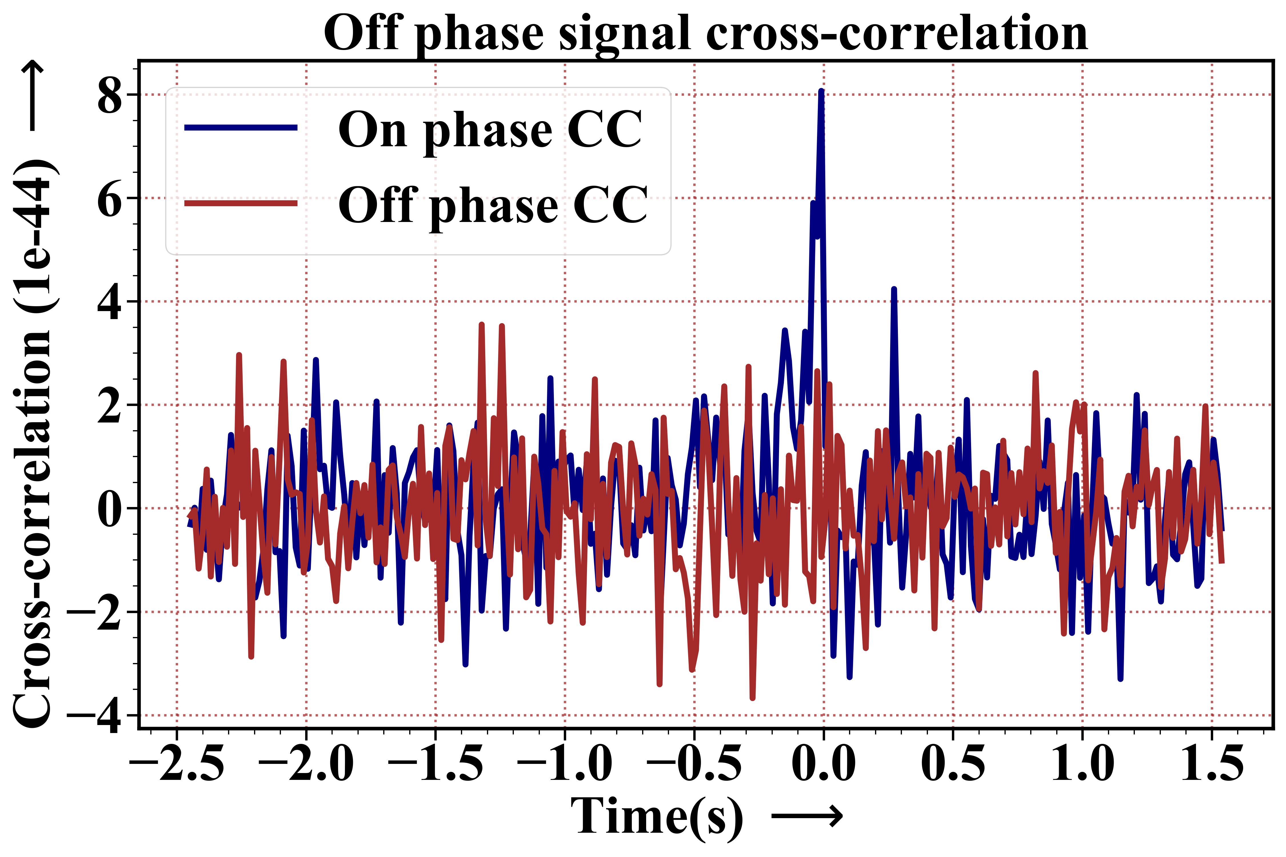
Figure 17: Cross-correlation between two signals, but not on phase with $\tau_{cc}=0.0625s$ vs cross-correlation of two signals on phase. It is evident that non-overlapping cross-correlation does not produce a nice cross-correlation signal.

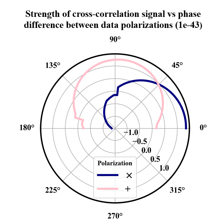
Figure 18: Polar plot showing the strength of the cross-correlation signal (the peak strength) with variation in phase-shift (due to lensing) of the GW signals while overlapping. Starting from the phase difference of zero, the cross-polarization signal goes down monotonically. The plus polarization signal, however, first increases and then decreases. When the cross-polarization signal is close to zero, the plus polarization signal is at max. The curve gets a sudden jump/fall when the noise cross-correlation is larger than the signal cross-correlation.

The strength of the cross-correlation signal when two signals are not lensed i.e. have different parameters is skipped, because we already have a similar plot i.e. fig. 11 shows that when the parameters of the two signals match, we obtain the tallest peak of the summed lensing SNR.

Appendix B Formalism for parameter estimation in case of multiple images

The cross-correlation technique can be applied between any two data pieces together and the lensing SNR would tell us about the significance of the event as lensed. However, this lensing detection technique can incorporate more than two images. The cross-correlation would be in between ${}^{3}C_{2}$ combinations given the data from one detector. Say for 3 images observed, we have three data pieces and then try to infer four degenerate parameters ($\sqrt{\mu_{1}},\sqrt{\mu_{2}},\sqrt{\mu_{3}},d_{l}$) out of it is pointless.

Thus we formulate a new likelihood function that takes these three data pieces as inputs and infers three parameters from it. These three parameters are: $d_{l}$ i.e. the true luminosity distance of the source, $\sqrt{\mu_{r2}}$ and $\sqrt{\mu_{r3}}$ giving the relative magnification of the second and third images with respect to the first image. The likelihood function now appears as,

$$-\log(L)=\frac{(d_{1}-h^{m}_{1})^{2}}{2\sigma_{n1}^{2}} +\frac{\log(2\pi\sigma_{n1}^{2})}{2}+\frac{(d_{2}-h^{m}_{2})^{2}}{2\sigma_{n2}^{2}}$$

$$+\frac{\log(2\pi\sigma_{n2}^{2})}{2}+\frac{(d_{3}-h^{m}_{3})^{2}}{2\sigma_{n3}^{2}}+\frac{\log(2\pi\sigma_{n3}^{2})}{2}$$ (21)

with $h^{m}_{1}=h_{1}^{ul}(d_{l})$ and $h^{m}_{2}=\sqrt{\mu_{r2}}h_{2}^{ul}(d_{l})$ and $h^{m}_{3}=\sqrt{\mu_{r3}}h_{3}^{ul}(d_{l})$ where the notations follow from equations 19 and 20. In fig. 19, we have shown the inference of those parameters from the data. The injection parameters are again quite well recovered.

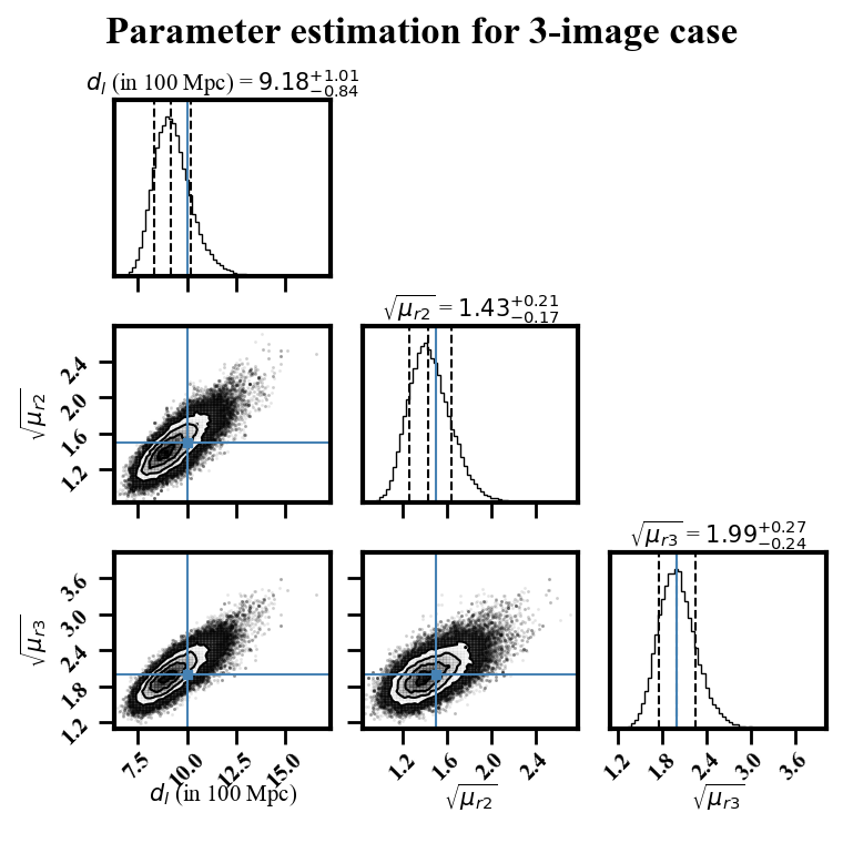
Figure 19: Inference of relative magnifications and luminosity distance for a 3-image scenario. The source and lens parameters are again degenerate; with three image signals, we can infer up to three parameters, here $d_{l}$ i.e. the true luminosity distance of the source, $\sqrt{\mu_{r2}}$ and $\sqrt{\mu_{r3}}$ giving the relative magnification of the second and third images with respect to the first image.

This technique can be extended to cases with any number of images with subsequent modifications needed in the likelihood function.

Appendix C Different noise realizations: how that throws off the lensing SNR and the parameter estimation

As can be seen in fig. 14 and fig. 15, the quality of the inference of the parameters depends on the signal strength. When the lensed signals have moderate match-filtered SNR, the inference standard deviation is small. However, with weak signals, parameters are estimated with large error bars. Not only do these kinds of estimations depend on the source parameters, but also strongly depend on the noise realizations when the signal is not that strong itself. As we tried our parameter estimation on moderate match-filtered SNR, our results were sometimes affected badly by some noise. We have shown the variation in the cross-correlation SNR and parameter estimation for different noise realizations in fig. 20 and fig. 21.

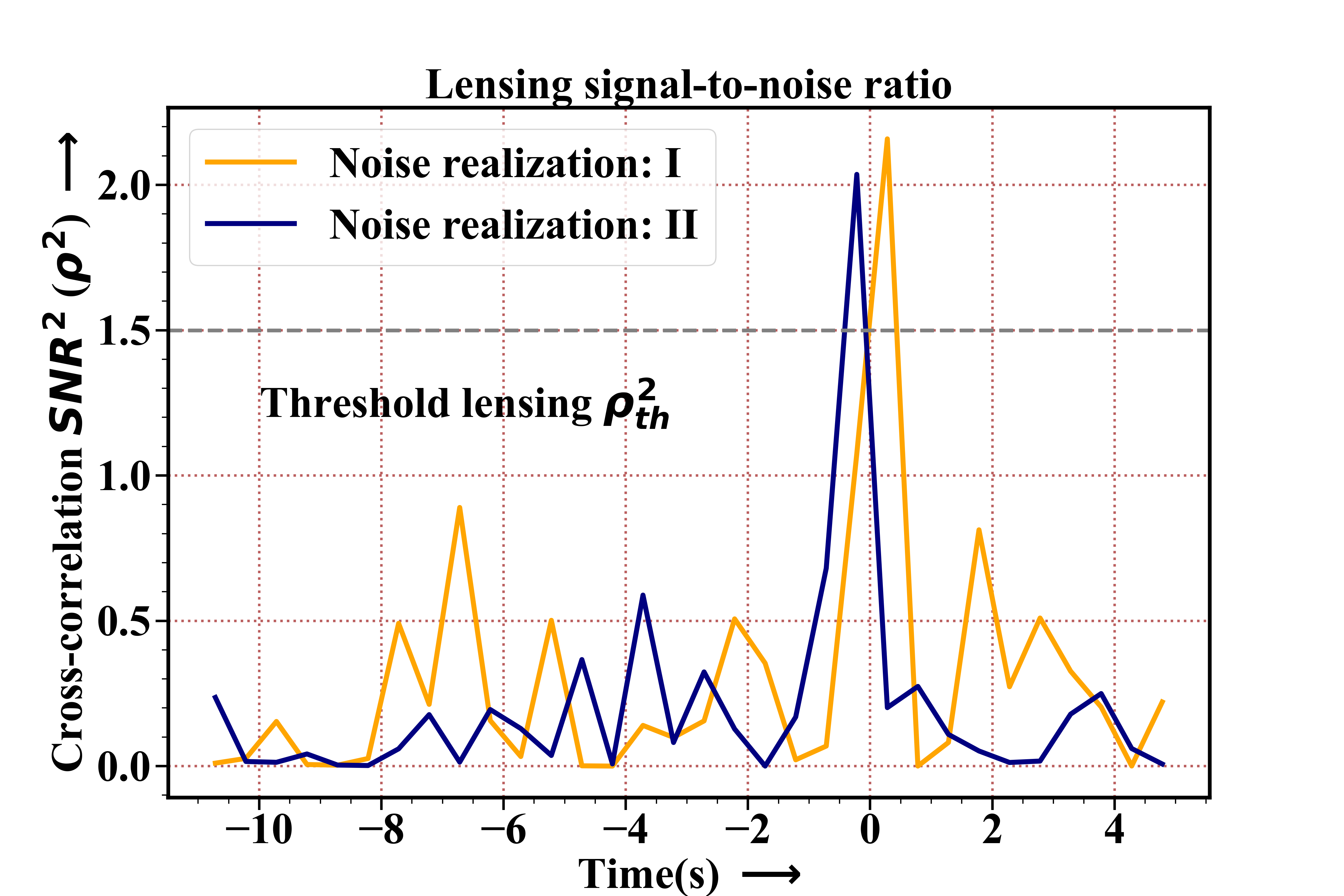
Figure 20: Lensing SNR for a different noise. We can see that the threshold is lowered to $\rho^{2}_{th}>1.5$. Although the peak corresponding to the signal (near $t=0s$) is much taller than the noise cross-correlations peaks, the overall peak height has diminished drastically. The cut-off is chosen according to the noise fluctuations as well the SNR timescale $\tau_{snr}$, here $\tau_{snr}=0.5s$. Thus we have no hard-bound prescription for the cut-off lensing SNR. The choice of an appropriate threshold lensing SNR ($\rho_{th}$) plays an essential role in the determination of the event significance.

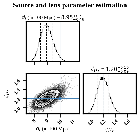
Figure 21: Source and lens characterization for a different noise. Although the inference of $\sqrt{\mu_{r}}$ is quite good (within 1-sigma around the median), the inference of $d_{l}$ is not that close. However, the inference of both parameters becomes better (with posteriors becoming narrower around the injection value) as the strength of the signal is increased.

For any peak having $\rho$ > $\rho_{th}$ in fig 20 can be checked to contain any lensed signal by taking a data piece around that time and using the Bayesian parameter estimation technique on it as discussed in section 6. Parameter estimation does not provide a bound on the parameter if there is no signal present. This shows the importance of setting a threshold of the lensing at such a height that all small and large peaks above the threshold are being tested thoroughly before rejection.

In fig. 21, we can see that although the underlying noise power spectral density (PSD) is the same, however, each noise realization impacts the inference when the signal strength is weak. The effect of noise realizations on the parameter estimation is diminished as we observe events with high SNR e.g. observation of a IMBH merger.

Appendix D max SNR vs sum SNR: In the use to extract parameter information from the signal

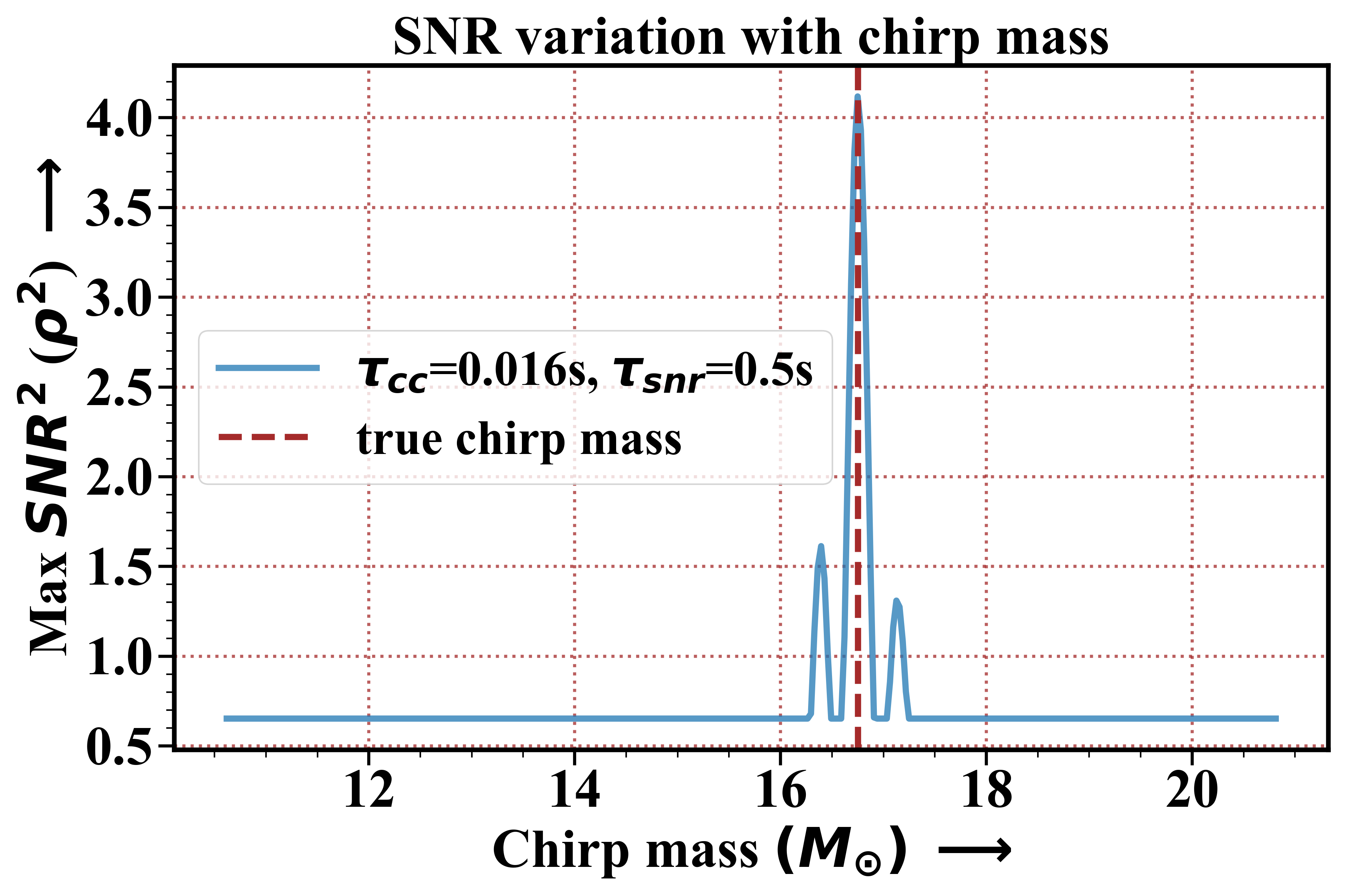
Figure 22: Variation of max SNR with chirp mass. The recovery of the injection of chirp mass is successful. The figure shows that max SNR can be a proxy to sum SNR to extract the source parameters accurately.

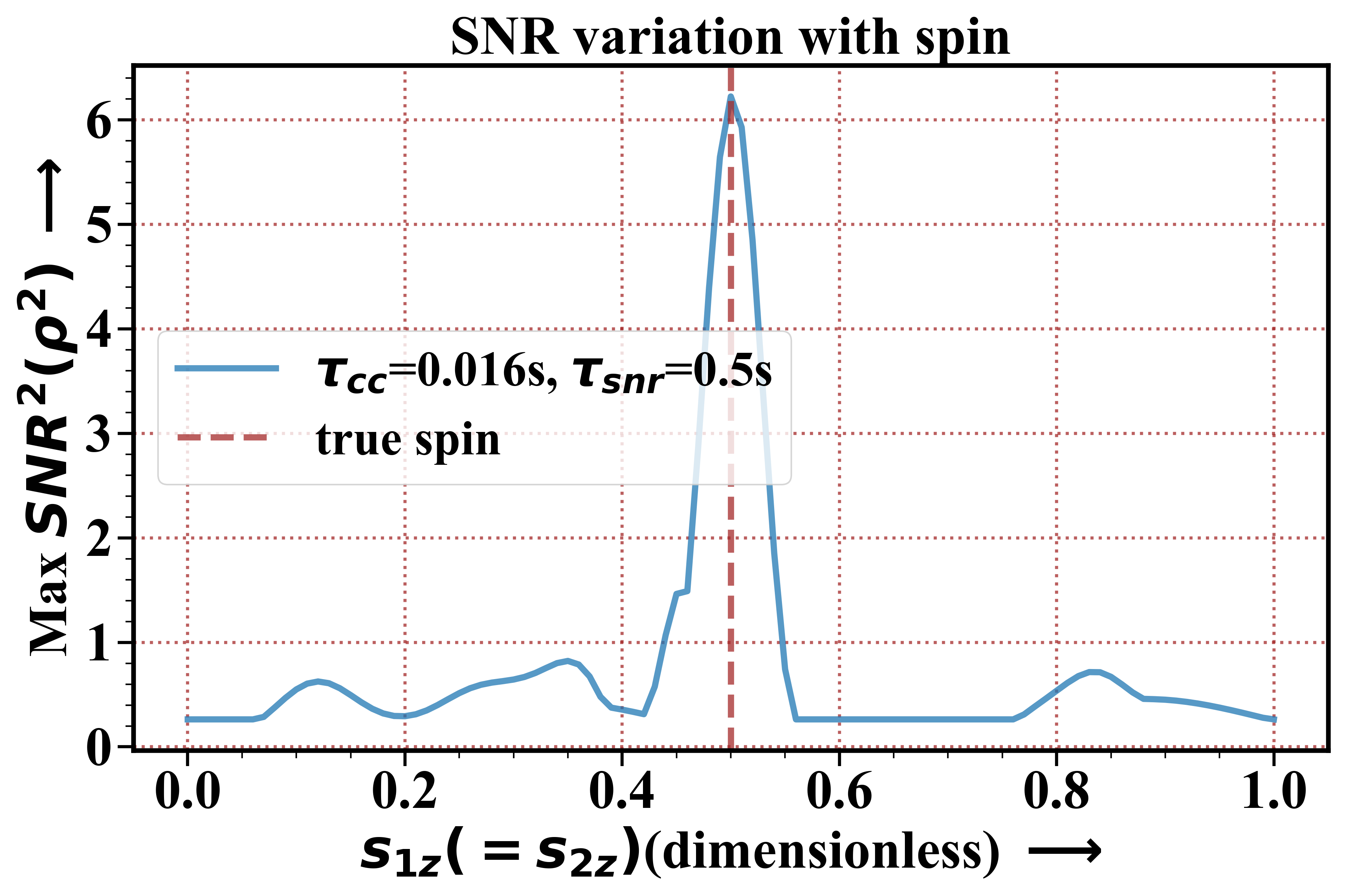
Figure 23: Variation of max lensing SNR with component black hole spin component towards orbital plane perpendicular direction. We can correctly infer the true spins of the binary black hole from this technique by using max SNR instead of sum SNR. Thus max SNR can act as a replacement, if not a better one, to the sum SNR technique.

In fig. 11, we have shown the inference of the injected source parameter from the signal cross-correlation. We did this by observing the total lensing SNR of the signal cross-correlation and one data-II was varied keeping other parameters fixed at the values same as that in data-I. However, that is not the only way to find the value of the parameter. Instead of plotting total lensing SNR, we can plot max lensing SNR with respect to a parameter and observe where a peak is obtained.

Fig. 22 shows that the max lensing SNR can also be used to find the injected chirp mass (given an apriori knowledge of other parameters). Similarly, 23 shows the variation of the max lensing SNR in black hole component spins, which shows that it is quite possible to infer the injected spin from the max lensing SNR peak. Thus, from the observations we can conclude that max lensing SNR can act aptly as a replacement for total lensing SNR.

For long signals, however, summed SNR will play a significant role in searching for lensed events because many points along the arrow of time will have a significant contribution to the SNR, and considering a single peak will cause loss of information.

References

- Abbott et al. (2016) Abbott B. P., et al., 2016, Phys. Rev. Lett., 116, 061102
- Abbott et al. (2018) Abbott B. P., et al., 2018, Living Rev. Rel., 21, 3
- Abbott et al. (2020) Abbott B. P., et al., 2020, Living Reviews in Relativity, 23
- Abbott et al. (2021) Abbott R., et al., 2021, 2112.06861
- Abbott et al. (2023a) Abbott R., et al., 2023a, Phys. Rev. X, 13, 011048
- Abbott et al. (2023b) Abbott R., et al., 2023b, Astrophys. J. Suppl., 267, 29
- Abbott et al. (2023c) Abbott R., et al., 2023c, Astrophys. J., 949, 76
- Allen & Romano (1999) Allen B., Romano J. D., 1999, Physical Review D, 59, 102001
- Astropy Collaboration et al. (2022) Astropy Collaboration et al., 2022, ApJ, 935, 167
- Balaudo et al. (2023) Balaudo A., Garoffolo A., Martinelli M., Mukherjee S., Silvestri A., 2023, JCAP, 06, 050
- Bartelmann (2010) Bartelmann M., 2010, Classical and Quantum Gravity, 27, 233001
- Basak et al. (2022) Basak S., Ganguly A., Haris K., Kapadia S., Mehta A. K., Ajith P., 2022, Astrophys. J., 926, L28
- Bayer et al. (2023) Bayer D., Koopmans L. V. E., McKean J. P., Vegetti S., Treu T., Fassnacht C. D., Glazebrook K., 2023, Monthly Notices of the Royal Astronomical Society, 523, 1326–1345
- Biesiada & Harikumar (2021) Biesiada M., Harikumar S., 2021, Universe, 7
- Biwer et al. (2019) Biwer C. M., Capano C. D., De S., Cabero M., Brown D. A., Nitz A. H., Raymond V., 2019, Publ. Astron. Soc. Pac., 131, 024503
- Buikema et al. (2020) Buikema A., et al., 2020, Physical Review D, 102
- Bulashenko & Ubach (2022) Bulashenko O., Ubach H., 2022, Journal of Cosmology and Astroparticle Physics, 2022, 022
- Cao et al. (2014) Cao Z., Li L.-F., Wang Y., 2014, Phys. Rev. D, 90, 062003
- Chakraborty & Mukherjee (2024a) Chakraborty A., Mukherjee S., 2024a, (Under preparation)
- Chakraborty & Mukherjee (2024b) Chakraborty A., Mukherjee S., 2024b, (Under preparation)
- Congedo & Taylor (2019) Congedo G., Taylor A., 2019, Phys. Rev. D, 99, 083526
- Cutler & Flanagan (1994) Cutler C., Flanagan E. E., 1994, Phys. Rev. D, 49, 2658
- Dai & Venumadhav (2017) Dai L., Venumadhav T., 2017, On the waveforms of gravitationally lensed gravitational waves (arXiv:1702.04724)
- Dai et al. (2017) Dai L., Venumadhav T., Sigurdson K., 2017, Phys. Rev. D, 95, 044011
- Dhurandhar et al. (2008) Dhurandhar S., Krishnan B., Mukhopadhyay H., Whelan J. T., 2008, Phys. Rev. D, 77, 082001
- Dideron et al. (2023) Dideron G., Mukherjee S., Lehner L., 2023, Physical Review D, 107
- Diego et al. (2021) Diego J., Broadhurst T., Smoot G., 2021, Physical Review D, 104
- Einstein (1915) Einstein A., 1915, Sitzungsber. Preuss. Akad. Wiss. Berlin (Math. Phys. ), 1915, 844
- Ezquiaga et al. (2021) Ezquiaga J. M., Holz D. E., Hu W., Lagos M., Wald R. M., 2021, Physical Review D, 103
- Foreman-Mackey (2016) Foreman-Mackey D., 2016, The Journal of Open Source Software, 1, 24
- Foreman-Mackey et al. (2013) Foreman-Mackey D., Hogg D. W., Lang D., Goodman J., 2013, Publications of the Astronomical Society of the Pacific, 125, 306–312
- Goyal et al. (2021) Goyal S., Haris K., Mehta A. K., Ajith P., 2021, Phys. Rev. D, 103, 024038
- Grespan & Biesiada (2023) Grespan M., Biesiada M., 2023, Universe, 9, 200
- Hall (2022) Hall E. D., 2022, Galaxies, 10
- Harris et al. (2020) Harris C. R., et al., 2020, Nature, 585, 357
- Hunter (2007) Hunter J. D., 2007, Computing in Science & Engineering, 9, 90
- Janquart et al. (2021) Janquart J., Hannuksela O. A., Haris K., Van Den Broeck C., 2021, Monthly Notices of the Royal Astronomical Society, 506, 5430
- Janquart et al. (2023) Janquart J., et al., 2023, Monthly Notices of the Royal Astronomical Society, 526, 3832
- Jung & Shin (2019) Jung S., Shin C. S., 2019, Phys. Rev. Lett., 122, 041103
- Khan et al. (2016) Khan S., Husa S., Hannam M., Ohme F., Pürrer M., Jiménez Forteza X., Bohé A., 2016, Phys. Rev. D, 93, 044007
- LIGO Scientific Collaboration et al. (2018) LIGO Scientific Collaboration Virgo Collaboration KAGRA Collaboration 2018, LVK Algorithm Library - LALSuite, Free software (GPL), doi:10.7935/GT1W-FZ16
- Li et al. (2018) Li S.-S., Mao S., Zhao Y., Lu Y., 2018, Monthly Notices of the Royal Astronomical Society, 476, 2220
- Li et al. (2023) Li A. K. Y., Lo R. K. L., Sachdev S., Chan J. C. L., Lin E. T., Li T. G. F., Weinstein A. J., 2023, Phys. Rev. D, 107, 123014
- Lo & Magaña Hernandez (2023) Lo R. K. L., Magaña Hernandez I., 2023, Phys. Rev. D, 107, 123015
- Macleod et al. (2021) Macleod D. M., Areeda J. S., Coughlin S. B., Massinger T. J., Urban A. L., 2021, SoftwareX, 13, 100657
- Martynov et al. (2016) Martynov D., et al., 2016, Physical Review D, 93
- Matsunaga & Yamamoto (2006) Matsunaga N., Yamamoto K., 2006, JCAP, 01, 023
- McIsaac et al. (2020) McIsaac C., Keitel D., Collett T., Harry I., Mozzon S., Edy O., Bacon D., 2020, Phys. Rev. D, 102, 084031
- Meena & Bagla (2019) Meena A. K., Bagla J. S., 2019, Monthly Notices of the Royal Astronomical Society, 492, 1127–1134
- Mpetha et al. (2023) Mpetha C. T., Congedo G., Taylor A., 2023, Phys. Rev. D, 107, 103518
- Mukherjee et al. (2020a) Mukherjee S., Wandelt B. D., Silk J., 2020a, Phys. Rev. D, 101, 103509
- Mukherjee et al. (2020b) Mukherjee S., Wandelt B. D., Silk J., 2020b, Mon. Not. Roy. Astron. Soc., 494, 1956
- Mukherjee et al. (2021) Mukherjee S., Broadhurst T., Diego J. M., Silk J., Smoot G. F., 2021, Monthly Notices of the Royal Astronomical Society, 506, 3751
- Nakamura (1998) Nakamura T. T., 1998, Phys. Rev. Lett., 80, 1138
- Narola et al. (2023) Narola H., Janquart J., Haegel L., Haris K., Hannuksela O. A., Van Den Broeck C., 2023, arXiv
- Ng et al. (2018) Ng K. K. Y., Wong K. W. K., Broadhurst T., Li T. G. F., 2018, Phys. Rev. D, 97, 023012
- Nitz et al. (2024) Nitz A., et al., 2024, gwastro/pycbc: v2.3.3 release of PyCBC, doi:10.5281/zenodo.10473621, https://doi.org/10.5281/zenodo.10473621
- Oguri (2018) Oguri M., 2018, Monthly Notices of the Royal Astronomical Society, 480, 3842
- Pankow et al. (2018) Pankow C., Chase E. A., Coughlin S., Zevin M., Kalogera V., 2018, The Astrophysical Journal Letters, 854, L25
- Poisson & Will (1995) Poisson E., Will C. M., 1995, Phys. Rev. D, 52, 848
- Punturo et al. (2010) Punturo M., et al., 2010, Class. Quant. Grav., 27, 194002
- Romano & Cornish (2017) Romano J. D., Cornish N. J., 2017, Living Reviews in Relativity, 20
- Savastano et al. (2023) Savastano S., Tambalo G., Villarrubia-Rojo H., Zumalacárregui M., 2023, Phys. Rev. D, 108, 103532
- Schneider et al. (1992) Schneider P., Ehlers J., Falco E. E., 1992, Gravitational Lenses, doi:10.1007/978-3-662-03758-4.
- Shukla et al. (2023) Shukla S. R., Pathak L., Sengupta A. S., 2023, How I wonder where you are: pinpointing coalescing binary neutron star sources with the IGWN, including LIGO-Aundha (arXiv:2311.15695)
- Smith et al. (2017) Smith G. P., et al., 2017, Proceedings of the International Astronomical Union, 13, 98–102
- Smith et al. (2018) Smith G. P., Jauzac M., Veitch J., Farr W. M., Massey R., Richard J., 2018, Monthly Notices of the Royal Astronomical Society, 475, 3823
- Takahashi & Nakamura (2003) Takahashi R., Nakamura T., 2003, The Astrophysical Journal, 595, 1039
- Tambalo et al. (2023) Tambalo G., Zumalacárregui M., Dai L., Cheung M. H.-Y., 2023, Phys. Rev. D, 108, 043527
- The LIGO Scientific Collaboration et al. (2023) The LIGO Scientific Collaboration et al., 2023, arXiv e-prints, p. arXiv:2304.08393
- Virtanen et al. (2020) Virtanen P., et al., 2020, Nature Methods, 17, 261
- Wambsganss (2006) Wambsganss J., 2006, in Françoise J.-P., Naber G. L., Tsun T. S., eds, , Encyclopedia of Mathematical Physics. Academic Press, Oxford, pp 567–575, doi:https://doi.org/10.1016/B0-12-512666-2/00067-5
- Wang et al. (1996) Wang Y., Stebbins A., Turner E. L., 1996, Phys. Rev. Lett., 77, 2875
- Wright & Hendry (2022) Wright M., Hendry M., 2022, ApJ, 935, 68
- Çalışkan et al. (2023a) Çalışkan M., Ji L., Cotesta R., Berti E., Kamionkowski M., Marsat S., 2023a, Phys. Rev. D, 107, 043029
- Çalışkan et al. (2023b) Çalışkan M., Ezquiaga J. M., Hannuksela O. A., Holz D. E., 2023b, Phys. Rev. D, 107, 063023
- Çalışkan et al. (2023c) Çalışkan M., Anil Kumar N., Ji L., Ezquiaga J. M., Cotesta R., Berti E., Kamionkowski M., 2023c, Phys. Rev. D, 108, 123543