jfarebro@cs.mcgill.ca, aviralkumar@google.com, rishabhagarwal@google.com
Stop Regressing: Training Value Functions via Classification for Scalable Deep RL
Abstract
Value functions are a central component of deep reinforcement learning (RL). These functions, parameterized by neural networks, are trained using a mean squared error regression objective to match bootstrapped target values. However, scaling value-based RL methods that use regression to large networks, such as high-capacity Transformers, has proven challenging. This difficulty is in stark contrast to supervised learning: by leveraging a cross-entropy classification loss, supervised methods have scaled reliably to massive networks. Observing this discrepancy, in this paper, we investigate whether the scalability of deep RL can also be improved simply by using classification in place of regression for training value functions. We demonstrate that value functions trained with categorical cross-entropy significantly improves performance and scalability in a variety of domains. These include: single-task RL on Atari 2600 games with SoftMoEs, multi-task RL on Atari with large-scale ResNets, robotic manipulation with Q-transformers, playing Chess without search, and a language-agent Wordle task with high-capacity Transformers, achieving state-of-the-art results on these domains. Through careful analysis, we show that the benefits of categorical cross-entropy primarily stem from its ability to mitigate issues inherent to value-based RL, such as noisy targets and non-stationarity. Overall, we argue that a simple shift to training value functions with categorical cross-entropy can yield substantial improvements in the scalability of deep RL at little-to-no cost.
1 Introduction
A clear pattern emerges in deep learning breakthroughs – from AlexNet (Krizhevsky et al., 2012) to Transformers (Vaswani et al., 2017) – classification problems seem to be particularly amenable to effective training with large neural networks. Even in scenarios where a regression approach appears natural, framing the problem instead as a classification problem often improves performance (Torgo and Gama, 1996; Rothe et al., 2018; Rogez et al., 2019). This involves converting real-valued targets into categorical labels and minimizing categorical cross-entropy rather than the mean-squared error. Several hypotheses have been put forward to explain the superiority of this approach, including stable gradients (Imani and White, 2018; Imani et al., 2024), better representations (Zhang et al., 2023), implicit bias (Stewart et al., 2023), and dealing with imbalanced data (Pintea et al., 2023) – suggesting their potential utility beyond supervised regression.
Unlike trends in supervised learning, value-based reinforcement learning (RL) methods primarily rely on regression. For example, deep RL methods such as deep Q-learning (Mnih et al., 2015) and actor-critic (Mnih et al., 2016) use a regression loss, such as mean-squared error, to train a value function from continuous scalar targets. While these value-based deep RL methods, powered by regression losses, have led to high-profile results (Silver et al., 2017), it has been challenging to scale them up to large networks, such as high-capacity transformers. This lack of scalability has been attributed to several issues (Kumar et al., 2021, 2022; Agarwal et al., 2021; Lyle et al., 2022; Le Lan et al., 2023; Obando-Ceron et al., 2024), but what if simply reframing the regression problem as classification can enable the same level of scalability achieved in supervised learning?
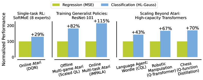
In this paper, we perform an extensive study to answer this question by assessing the efficacy of various methods for deriving classification labels for training a value-function with a categorical cross-entropy loss. Our findings reveal that training value-functions with cross-entropy substantially improves the performance, robustness, and scalability of deep RL methods (Figure 1) compared to traditional regression-based approaches. The most notable method (HL-Gauss; Imani and White, 2018) leads to consistently 30% better performance when scaling parameters with Mixture-of-Experts in single-task RL on Atari (Obando-Ceron et al., 2024); performance in multi-task setups on Atari (Kumar et al., 2023; Ali Taïga et al., 2023); % better performance in the language-agent task of Wordle (Snell et al., 2023); % improvement for playing chess without search (Ruoss et al., 2024); and % better performance on large-scale robotic manipulation with transformers (Chebotar et al., 2023). The consistent trend across diverse domains, network architectures, and algorithms highlights the substantial benefits of treating regression as classification in deep RL, underscoring its potential as a pivotal component as we move towards scaling up value-based RL.
With strong empirical results to support the use of cross-entropy as a “drop-in” replacement for the mean squared error (MSE) regression loss in deep RL, we also attempt to understand the source of these empirical gains. Based on careful diagnostic experiments, we show that the categorical cross-entropy loss offers a number of benefits over mean-squared regression. Our analysis suggests that the categorical cross-entropy loss mitigates several issues inherent to deep RL, including robustness to noisy targets and allowing the network to better use its capacity to fit non-stationary targets. These findings not only help explain the strong empirical advantages of categorical cross-entropy in deep RL but also provide insight into developing more effective learning algorithms for the field.
2 Preliminaries and Background

Regression as classification. We take a probabilistic view on regression where given input we seek to model the target as a conditional distribution for some fixed variance and predictor function parameterized by the vector . The maximum likelihood estimator for data is characterized by the mean-squared error (MSE) objective,
with the optimal predictor being .
Instead of learning the mean of the conditional distribution directly, an alternate approach is to learn a distribution over the target value, and then, recover the prediction as a statistic of the distribution. To this end, we will construct the target distribution with probability density function such that our scalar target can be recovered as the mean of this distribution . We can now frame the regression problem as learning a parameterized distribution that minimizes the KL divergence to the target ,
| (2.1) |
which is the cross-entropy objective. Finally, our prediction can be recovered as .
Given this new problem formulation, in order to transform the distribution learning problem into a tractable loss we restrict to the set of categorical distributions supported on with evenly spaced locations or “classes”, defined as,
| (2.2) |
where is the probability associated with location and is the Dirac delta function at location . The final hurdle is to define a procedure to construct the target distribution and its associated projection onto the set of categorical distributions . We defer this discussion to §3 where we discuss various methods for performing these steps in the context of RL.
Reinforcement Learning (RL). We consider the reinforcement learning (RL) problem where an agent interacts with an environment by taking an action in the current state and subsequently prescribed a reward before transitioning to the next state according to the environment transition probabilities. The return numerically describes the quality of a sequence of actions as the cumulative discounted sum of rewards where is the discount factor. The agent’s goal is to learn the policy that maximizes the expected return. The action-value function allows us to query the expected return from taking action in state and following policy thereafter: .
Deep Q-Networks (DQN; Mnih et al., 2015) proposes to learn the approximately optimal state-action value function with a neural network parameterized by . Specifically, DQN minimizes the mean-squared temporal difference (TD) error from transitions sampled from dataset ,
| (2.3) |
where is a slow moving copy of the parameters that parameterize the “target network” and
is the sample version of the Bellman optimality operator which defines our scalar regression target. Most deep RL algorithms that learn value functions use variations of this basic recipe, notably regressing to predictions obtained from a target value network.
In addition to the standard online RL problem setting, we also explore the offline RL setting where we train agents using a fixed dataset of environment interactions (Agarwal et al., 2020; Levine et al., 2020). One widely-used offline RL method is CQL (Kumar et al., 2020) that jointly optimizes the TD error with a behavior regularization loss with strength , using the following training objective:
| (2.4) |
This work aims to replace the fundamental mean-squared TD-error objective with a classification-style cross-entropy loss for both value-based and actor-critic methods, in both offline and online domains.
3 Value-Based RL with Classification
In this section, we describe our approach to cast the regression problem appearing in TD-learning as a classification problem. Concretely, instead of minimizing the squared distance between the scalar Q-value and its TD target (Equation 2.3) we will instead minimize the distance between categorical distributions representing these quantities. To employ this approach, we will first define the categorical representation for the action-value function .
Categorical Representation. We choose to represent as the expected value of a categorical distribution . This distribution is parameterized by probabilities for each location or “class” which are derived from the logits through the softmax function:
To employ the cross-entropy loss (Equation 2.1) for TD learning, it is necessary that the target distribution is also a categorical distribution, supported on the same locations . This allows for the direct computation of the cross-entropy loss as:
| (3.1) |
where the target probabilities are defined such that . In the subsequent sections, we explore two strategies for obtaining the target probabilities .

3.1 Constructing Categorical Distributions from Scalars
The first set of methods we outline will project the scalar target onto the categorical distribution supported on . A prevalent but naïve approach for the projection step involves discretizing the scalar into one of bins where represents the center of the bin. The resulting one-hot distribution is “lossy” and induces errors in the -function. These errors would compound as more Bellman backups are performed, resulting in more biased estimates, and likely worse performance. To combat this, we first consider the “two-hot” approach (Schrittwieser et al., 2020) that represents a scalar target exactly via a unique categorical distribution that puts non-zero densities on two locations that the target lies between (see Figure 3; Left).
A Two-Hot Categorical Distribution. Let and be the locations which lower and upper-bound the TD target . Then, the probability, and , put on these locations is:
| (3.2) |
For all other locations, the probability prescribed by the categorical distribution is exactly zero. In principle, this Two-Hot transformation provides a uniquely identifiable and a non-lossy representation of the scalar TD target to a categorical distribution. However, Two-Hot does not fully harness the ordinal structure of discrete regression. Specifically, the classes are not independent and instead have a natural ordering, where each class intrinsically relates to its neighbors.
The class of Histogram Losses introduced by Imani and White (2018) seeks to exploit the ordinal structure of the regression task by distributing probability mass to neighboring bins – akin to label smoothing in supervised classification (Szegedy et al., 2016). This is done by transforming a noisy version of the target value into a categorical distribution where probability mass can span multiple bins near the target (See Figure 3; Center), rather than being restricted to two locations.
Histograms as Categorical Distributions. Formally, define the random variable with probability density and cumulative distribution function whose expectation is . We can project the distribution onto the histogram with bins of width centered at by integrating over the interval to obtain the probabilities,
| (3.3) |
We now have a choice for the distribution . We follow the suggestion of Imani and White (2018) in using the Gaussian distribution where the variance is a hyper-parameter that can control the amount of label smoothing applied to the resulting categorical distribution. We refer to this method as HL-Gauss.
How should we tune in practice? HL-Gauss requires tuning the standard deviation , in addition to the bin width and distribution range . 99.7% of the samples obtained by sampling from a standard Normal distribution should lie within three standard deviations of the mean with high confidence, which corresponds to approximately bins. Thus, a more interpretable hyper-parameter that we recommend tuning is : setting it to distributes most of the probability mass to neighbouring locations for a mean value centered at one of the bins. Unless specified otherwise, we set for our experiments, which distributes mass to approximately locations.
3.2 Modelling the Categorical Return Distribution
In the previous section, we chose to construct a target distribution from the usual scalar regression target representing the expected return. Another option is to directly model the distribution over future returns using our categorical model , as done in distributional RL (Bellemare et al., 2023). Notably, C51 (Bellemare et al., 2017), an early distributional RL approach, use the categorical representation along with minimizing the cross-entropy between the predicted distribution and the distributional analogue of the TD target. To this end, we also investigate C51 as an alternative to Two-Hot and HL-Gauss for constructing the target distribution for our cross-entropy objective.
Categorical Distributional RL. The first step to modelling the categorical return distribution is to define the analogous stochastic distributional Bellman operator on ,
where . As we can see, the stochastic distributional Bellman operator has the effect of shifting and scaling the locations necessitating the categorical projection, first introduced by Bellemare et al. (2017). At a high level, this projection distributes probabilities proportionally to the immediate neighboring locations (See Figure 3; Right). To help us identify these neighboring locations we define and . Now the probabilities for location can be written as,
| (3.4) | ||||
For a complete exposition of the categorical projection, see Bellemare et al. (2023, Chapter 5).
4 Evaluating Classification Losses in RL
The goal of our experiments in this section is to evaluate the efficacy of the various target distributions discussed in Section 3 combined with the categorical cross-entropy loss (3.1) in improving performance and scalability of value-based deep RL on a variety of problems. This includes several single-task and multi-task RL problems on Atari 2600 games as well as domains beyond Atari including language agents, chess, and robotic manipulation. These tasks consist of both online and offline RL problems. For each task, we instantiate our cross-entropy losses in conjunction with a strong value-based RL approach previously evaluated on that task. Full experimental methodologies including hyperparameters for each domain we consider can be found in Appendix B.
4.1 Single-Task RL on Atari Games
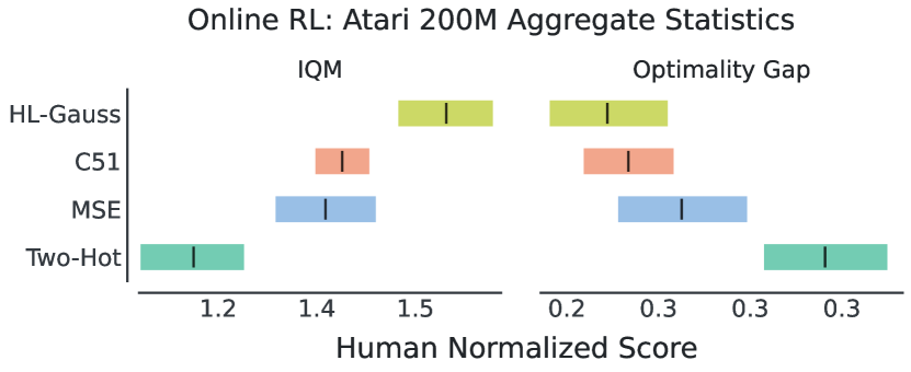
We first evaluate the efficacy of HL-Gauss, Two-Hot, and C51 (Bellemare et al., 2017) – an instantiation of categorical distributional RL, on the Arcade Learning Environment (Bellemare et al., 2013). For our regression baseline we train DQN (Mnih et al., 2015) on the mean-squared error TD objective which has been shown to outperform other regression based losses (Ceron and Castro, 2021). Each method is trained with the Adam optimizer, which has been shown to reduce the performance discrepancy between regression-based methods and distributional RL approaches (Agarwal et al., 2021).
Evaluation. Following the recommendations by Agarwal et al. (2021), we report the interquartile mean (IQM) normalized scores with 95% stratified bootstrap confidence intervals (CIs), aggregated across games with multiple seeds each. We report human-normalized aggregated scores across 60 Atari games for online RL. For offline RL, we report behavior-policy normalized scores aggregated across 17 games, following the protocol in Kumar et al. (2021).
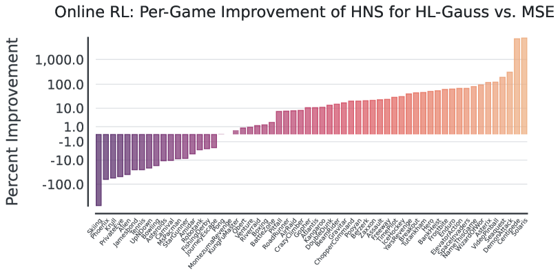
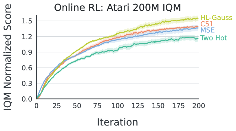
Online RL results. Following the setup of Mnih et al. (2015), we train DQN for 200M frames with the aforementioned losses. We report aggregated human-normalized IQM performance and optimality gap across 60 Atari games in Figure 4. Observe that HL-Gauss substantially outperforms the Two-Hot and MSE losses. Interestingly, HL-Gauss also improves upon categorical distributional RL (C51), despite not modelling the return distribution. This finding suggests that the loss (categorical cross-entropy) is perhaps the more crucial factor for C51, as compared to modelling the return distribution.
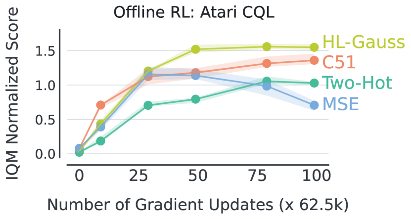
Offline RL results. The strong performance of HL-Gauss with online DQN, which involves learning from self-collected interactions, raises the question of whether it would also be effective in learning from offline datasets. To do so, we train agents with different losses on the 10% Atari DQN replay dataset (Agarwal et al., 2020) using CQL (§2) for 6.25M gradient steps. As shown in Figure 4, HL-Gauss and C51 consistently outperform MSE, while Two-Hot shows improved stability over MSE but underperforms other classification methods. Notably, HL-Gauss again surpasses C51 in this setting. Furthermore, consistent with the findings of Kumar et al. (2021), utilizing the mean squared regression loss results in performance degradation with prolonged training. However, cross-entropy losses (both HL-Gauss and C51) do not show such degradation and generally, remain stable.
4.2 Scaling Value-based RL to Large Networks
In supervised learning, particularly for language modeling (Kaplan et al., 2020), increasing the parameter count of a network typically improves performance. However, such scaling behavior remain elusive for value-based deep RL methods, where naive parameter scaling can hurt performance (Ali Taïga et al., 2023; Kumar et al., 2023; Obando-Ceron et al., 2024). To this end, we investigate the efficacy of our classification methods, as an alternative to MSE regression loss in deep RL, towards enabling better performance with parameter scaling for value-networks.
4.2.1 Scaling with Mixture-of-Experts
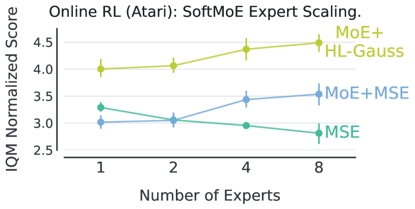
Recently, Obando-Ceron et al. (2024) demonstrate that while parameter scaling with convolutional networks hurts single-task RL performance on Atari, incorporating Mixture-of-Expert (MoE) modules in such networks improves performance. Following their setup, we replace the penultimate layer in the architecture employed by Impala (Espeholt et al., 2018) with a SoftMoE (Puigcerver et al., 2024) module and vary the number of experts in . Since each expert is a copy of the original penultimate layer, this layer’s parameter count increases by a factor equal to the number of experts. The only change we make is to replace the MSE loss in SoftMoE DQN, as employed by Obando-Ceron et al. (2024), with the HL-Gauss cross-entropy loss. We train on the same subset of 20 Atari games used by Obando-Ceron et al. (2024) and report aggregate results over five seeds in Figure 6.
As shown in Figure 6, we find that HL-Gauss consistently improves performance over MSE by a constant factor independent of the number of experts. One can also observe that SoftMoE + MSE seems to mitigate some of the negative scaling effects observed with MSE alone. As SoftMoE + MSE uses a softmax in the penultimate layer this could be providing similar benefits to using a classification loss but as we will later see these benefits alone cannot be explained by the addition of the softmax.
4.2.2 Training Generalist Policies with ResNets
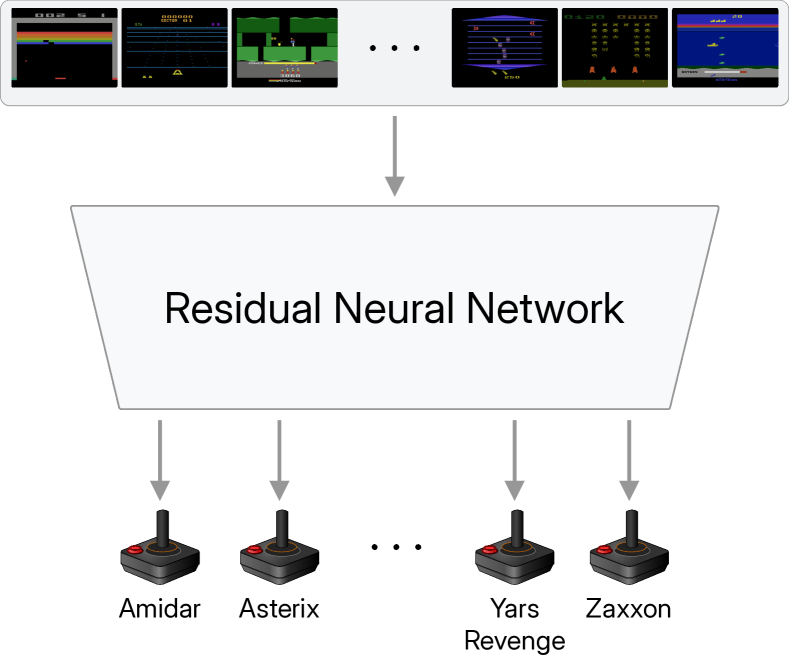
Next, we consider scaling value-based ResNets (He et al., 2016) in both offline and online settings to train a generalist video game-playing policy on Atari. In each case, we train a family of differently sized Q-networks for multi-task RL, and report performance as a function of the network size.
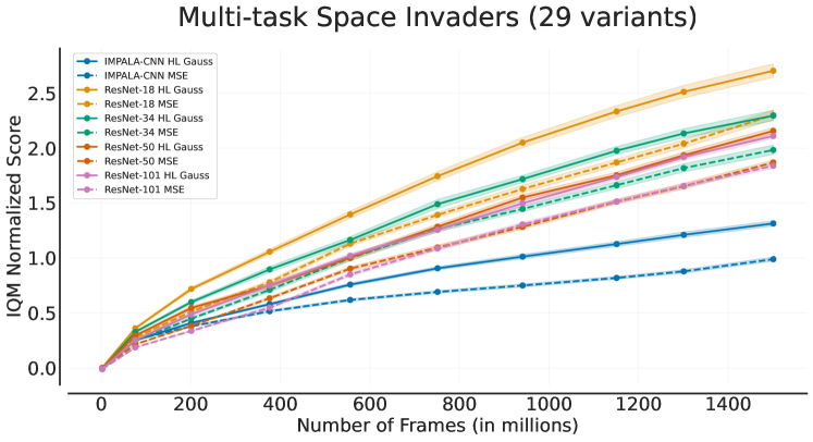
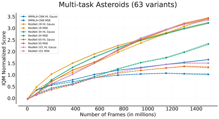
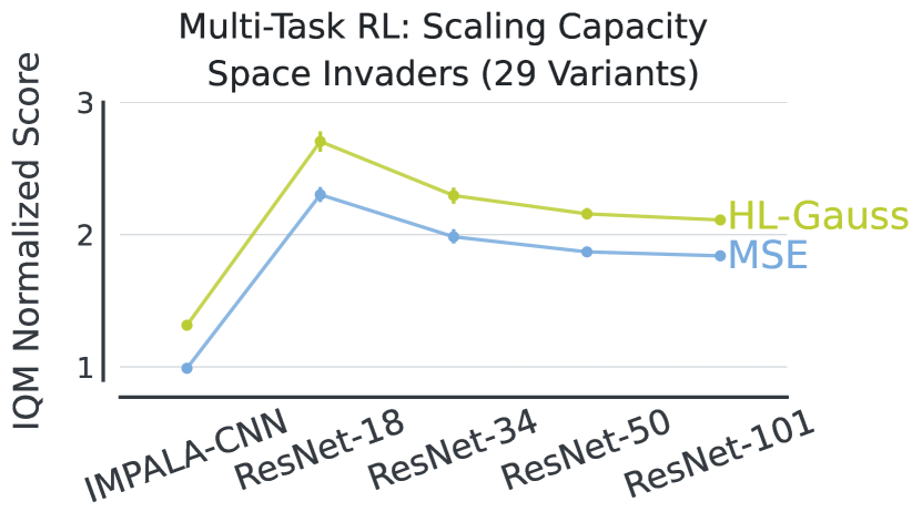
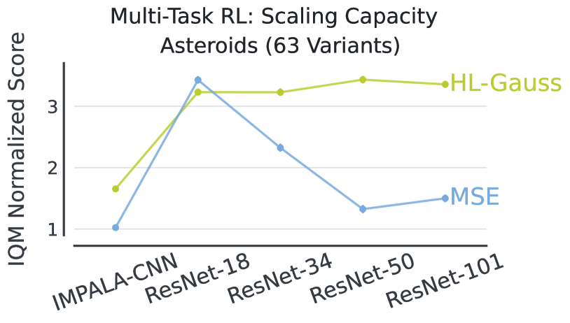
Multi-task Online RL. Following Ali Taïga et al. (2023), we train a multi-task policy capable of playing Atari game variants with different environment dynamics and rewards (Farebrother et al., 2018). We evaluate two Atari games: 63 variants for Asteroids and 29 variants for Space Invaders. We employ a distributed actor-critic method, IMPALA (Espeholt et al., 2018), and compare the standard MSE critic loss with the cross-entropy based HL-Gauss loss. Our experiments investigate the scaling properties of these losses when moving from Impala-CNN ( 2M parameters) to larger ResNets (He et al., 2016) up to ResNet-101 (44M parameters). We evaluate multi-task performance after training for 15 billion frames, and repeat each experiment with five seeds.
Results for Asteroids are presented in Figure 6, with additional results on Space Invaders presented in Figure D.4. We observe that in both environments HL-Gauss consistently outperforms MSE. Notably, HL-Gauss scales better, especially on Asteroids where it even slightly improves performance with larger networks beyond ResNet-18, while MSE performance significantly degrades.
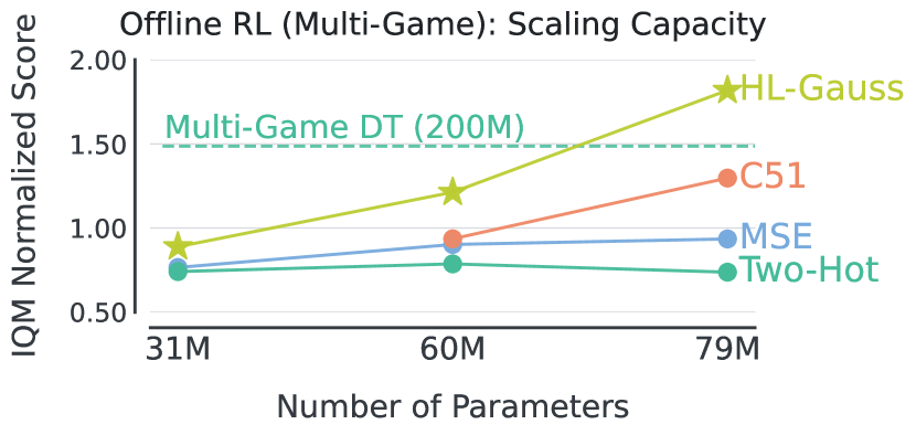
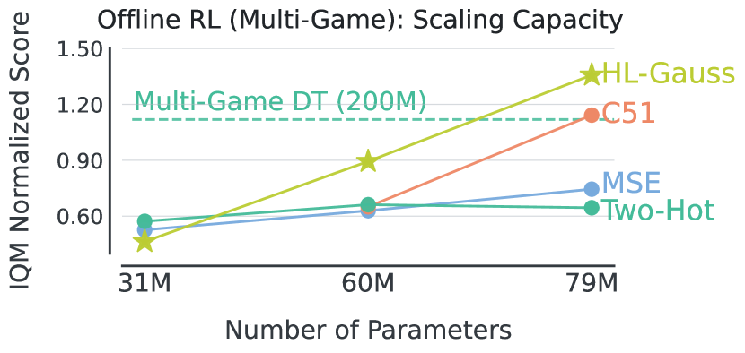
Multi-game Offline RL. We consider the the setup from Kumar et al. (2023), where we modify their recipe to use a non-distributional HL-Gauss loss, in place of distributional C51. Specifically, we train a single generalist policy to play 40 different Atari games simultaneously, when learning from a “near-optimal” training dataset, composed of replay buffers obtained from online RL agents trained independently on each game. This multi-game RL setup was originally proposed by Lee et al. (2022). The remaining design choices (e.g., feature normalization; the size of the network) are kept identical.
As shown in Figure 7, HL-Gauss scales even better than the C51 results from Kumar et al. (2023), resulting in an improvement of about over the best prior multi-game result available with ResNet-101 (80M parameters) as measured by the IQM human normalized score (Agarwal et al., 2021). Furthermore, while the performance of MSE regression losses typically plateaus upon increasing model capacity beyond ResNet-34, HL-Gauss is able to leverage this capacity to improve performance, indicating the efficacy of classification-based cross-entropy losses. Additionally, when normalizing against scores obtained by a DQN agent, we show in Figure D.4 that in addition to performance, the rate of improvement as the model scale increases tends to also be larger for the HL-Gauss loss compared to C51.
4.3 Value-Based RL with Transformers
Next, we evaluate the applicability of the HL-Gauss cross-entropy loss beyond Atari. To do so, we consider several tasks that utilize high-capacity Transformers, namely, a language-agent task of playing Wordle, playing Chess without inference-time search, and robotic manipulation.
4.3.1 Language Agent: Wordle
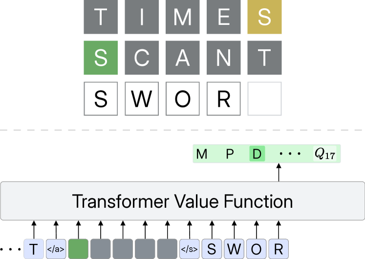
To evaluate whether classification losses enhance the performance of value-based RL approaches on language agent benchmarks, we compare HL-Gauss with MSE on the task of playing the game of Wordle111www.nytimes.com/games/wordle/index.html. Wordle is a word guessing game in which the agent gets 6 attempts to guess a word. Each turn the agent receives environment feedback about whether guessed letters are in the true word. The dynamics of this task are non-deterministic. More generally, the task follows a turn-based structure, reminiscent of dialogue tasks in natural language processing. This experiment is situated in the offline RL setting, where we utilize the dataset of suboptimal game-plays provided by Snell et al. (2023). Our goal is to train a GPT-like, decoder-only Transformer, with 125M parameters, representing the Q-network. See Figure 8 (left) for how the transformer model is used for playing this game.
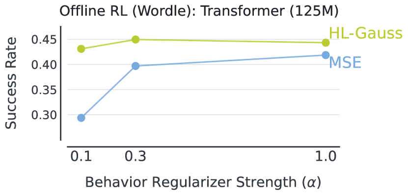
On this task, we train the language-based transformer for 20K gradient steps with an offline RL approach combining Q-learning updates from DQN with a CQL-style behavior regularizer (§2), which corresponds to standard next-token prediction loss (in this particular problem). As shown in Figure 8, HL-Gauss outperforms MSE, for multiple coefficients controlling the strength of CQL regularization.
4.3.2 Grandmaster-level Chess without Search
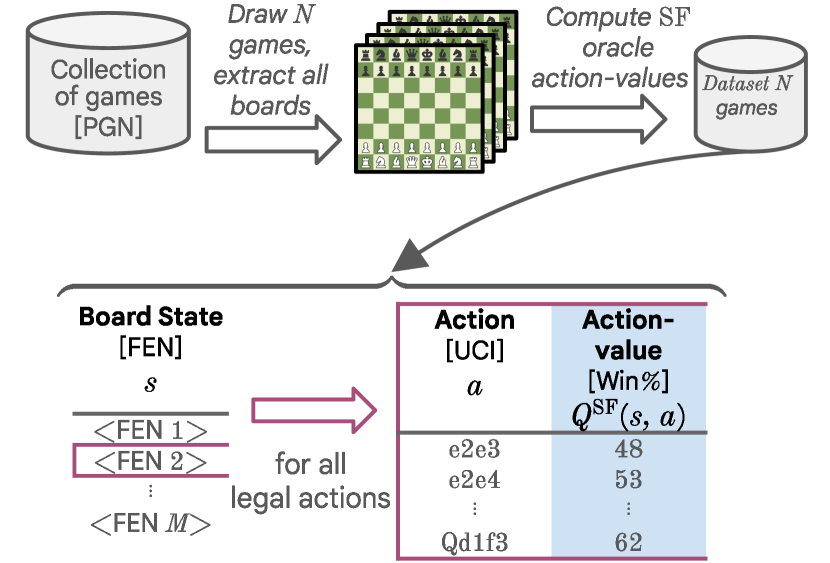
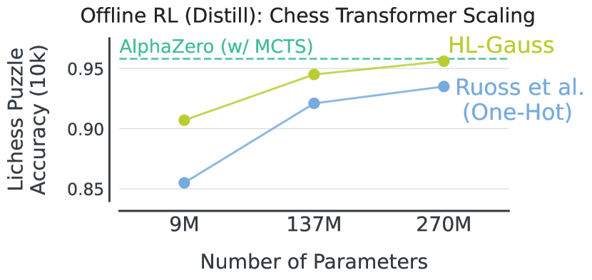
Transformers have demonstrated their effectiveness as general-purpose algorithm approximators, effectively amortizing expensive inference-time computation through distillation (Ruoss et al., 2024; Lehnert et al., 2024). In this context, we explore the potential benefits of using HL-Gauss to convert scalar action-values into classification targets for distilling a value-function. Using the setup of Ruoss et al. (2024), we evaluate HL-Gauss for distilling the action-value function of Stockfish 16 — the strongest available Chess engine that uses a combination of complex heuristics and explicit search — into a causal transformer. The distillation dataset comprises 10 million chess games annotated by the Stockfish engine, yielding 15 billion data points (Figure 9, left).
We train 3 transformer models of varying capacity (9M, 137M, and 270M parameters) on this dataset, using either HL-Gauss or 1-Hot classification targets. We omit MSE as Ruoss et al. (2024) demonstrate that 1-Hot targets outperform MSE on this task. The effectiveness of each model is evaluated based on its ability to solve 10,000 chess puzzles from Lichess, with success measured by the accuracy of the generated action sequences compared to known solutions. Both the setup and results are presented in Figure 9 (right). While the one-hot target with the 270M Transformer from Ruoss et al. (2024) outperformed an AlphaZero baseline without search, HL-Gauss closes the performance gap with the substantially stronger AlphaZero with 400 MCTS simulations (Schrittwieser et al., 2020).
4.3.3 Generalist Robotic Manipulation with Offline Data
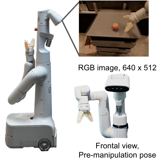
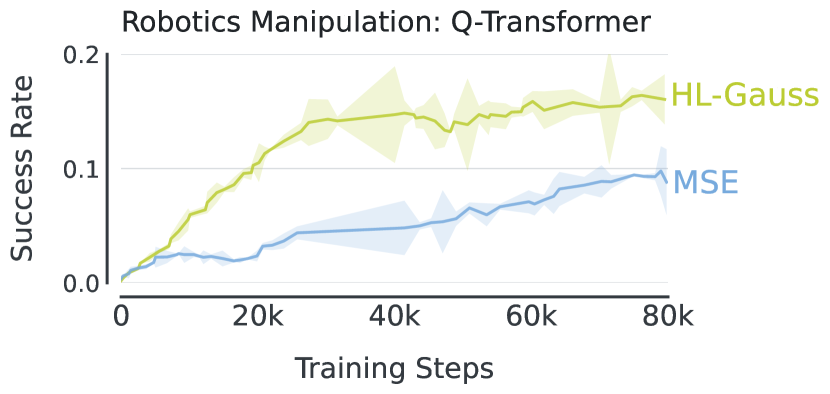
Finally, we evaluate whether cross-entropy losses can improve performance on a set of large-scale vision-based robotic manipulation control tasks from Chebotar et al. (2023). These tasks present a simulated 7-DoF mobile manipulator, placed in front of a countertop surface. The goal is to control this manipulator to successfully grasp and lift 17 different kitchen objects in the presence of distractor objects, clutter, and randomized initial poses. We generate a dataset of (successful and failed) episodes starting from a small amount of human-teleoperated demonstrations ( episodes) by replaying expert demonstrations with added sampled action noise, reminiscent of failed autonomously-collected rollouts obtained during deployment or evaluations of a behavioral cloning policy trained on the human demonstration data.
We train a Q-Transformer model with 60M parameters, following the recipe in Chebotar et al. (2023), but replace the MSE regression loss with the HL-Gauss classification loss. As shown in Figure 10, HL-Gauss results in higher peak performance over the regression baseline, while being much more sample-efficient, addressing a key limitation of the prior regression-based approach.
5 Why Does Classification Benefit RL?
Our experiments demonstrate that classification losses can significantly improve the performance and scalability of value-based deep RL. In this section, we perform controlled experiments to understand why classification benefits value-based RL. Specifically, we attempt to understand how the categorical cross-entropy loss can address several challenges specific to value-based RL including representation learning, stability, and robustness. We will also perform ablation experiments to uncover the reasons behind the superiority of HL-Gauss over other categorical targets.
5.1 Ablation Study: What Components of Classification Losses Matter?
Classification losses presented in this paper differ from traditional regression losses used in value-based RL in two ways: (1) parameterizing the output of the value-network to be a categorical distribution in place of a scalar, and (2) strategies for converting scalar targets into a categorical target. We will now understand the relative contribution of these steps towards the performance of cross-entropy losses.
5.1.1 Are Categorical Representations More Performant?
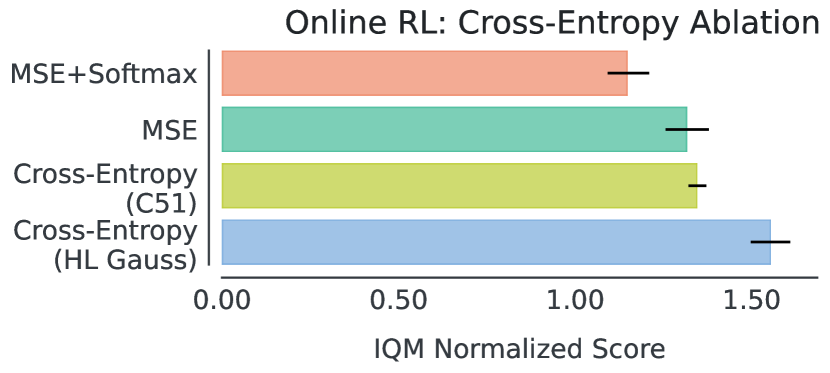
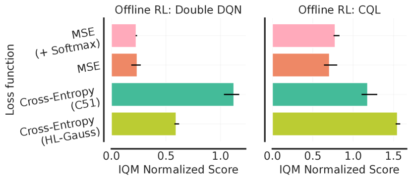
As discussed in §3.1, we parameterize the Q-network to output logits that are converted to probabilities of a categorical distribution by applying the “softmax” operator. Using softmax leads to bounded Q-values and bounded output gradients, which can possibly improve RL training stability (Hansen et al., 2024). To investigate whether our Q-value parameterization alone results in improved performance without needing a cross-entropy loss, we train Q-functions with the same parameterization as Eq (3.1) but with MSE. We do not observe any gains from using softmax in conjunction with the MSE loss in both online (Figure 12) and offline RL (Figure 12). This highlights that the use of the cross-entropy loss results in the bulk of the performance improvements.
5.1.2 Why Do Some Cross-Entropy Losses Work Better Than Others?
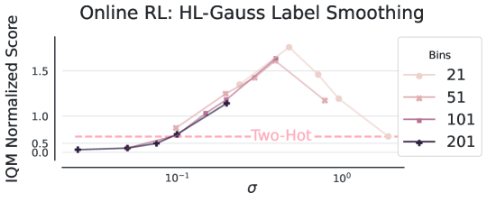
Our results indicate that HL-Gauss outperforms Two-Hot, despite both these methods using a cross-entropy loss. We hypothesize that the benefits of HL-Gauss could stem from two reasons: 1) HL-Gauss reduces overfitting by spreading probability mass to neighboring locations; and 2) HL-Gauss generalizes across a specific range of target values, exploiting ordinal structure in the regression problem. The first hypothesis would be more consistent with how label smoothing addresses overfitting in classification problems (Szegedy et al., 2016).
We test these hypotheses in the online RL setting across a subset of Atari games. To do so, we fix the value range while simultaneously varying the number of categorical bins in and the ratio of deviation to bin width in . We find that a wide range of values for HL-Gauss outperform Two-Hot, indicating that spreading probability mass to neighbouring locations likely results in less overfitting. Interestingly, we notice that the second hypothesis is also at play, as the optimal value of seems to be independent of number of bins, indicating that HL-Gauss generalizes best across a specific range of target values and is indeed leveraging the ordinal nature of the regression problem. Thus, the gains from HL-Gauss cannot be entirely attributed to overfitting, as is believed to be the case for label smoothing.
5.2 What Challenges Does Classification Address in Value-Based RL?
Having seen that the performance gains of cross-entropy losses stem from both the use of a categorical representation of values and distributed targets, we now attempt to understand which challenges in value-based RL cross-entropy losses address, or at least, partially alleviate.
5.2.1 Is Classification More Robust to Noisy Targets?
Classification is less prone to overfitting to noisy targets than regression, as it focuses on the categorical relationship between the input and target rather than their exact numerical relationship. We investigate whether classification could better deal with noise induced by stochasticity in RL.
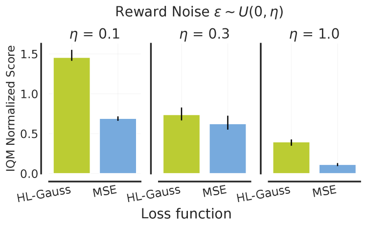
(a) Noisy Rewards. To test robustness of classification to stochasticity in rewards, we consider an offline RL setup where we add random noise , sampled uniformly from , to each dataset reward . We vary the noise scale and compare the performance of cross-entropy based HL-Gauss with the MSE loss. As shown in Figure 15, the performance of HL-Gauss degrades more gracefully than MSE as the noise scale increases.
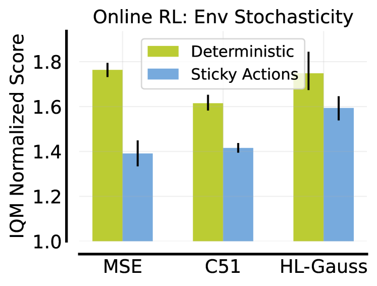
(b) Stochasticity in Dynamics. Following Machado et al. (2018), our Atari experiments use sticky actions — with 25% probability, the environment will execute the previous action again, instead of the agent’s executed action — resulting in non-deterministic dynamics. Here, we turn off sticky actions to compare different losses on deterministic Atari (60 games). As shown in Figure 15, while cross-entropy based HL-Gauss outperforms MSE with stochastic dynamics, they perform comparably under deterministic dynamics while outperforming distributional C51.
Overall, the benefits of cross-entropy losses can be partly attributed to less overfitting to noisy targets, an issue inherent to RL environments with stochastic dynamics or rewards. Such stochasticity issues may also arise as a result of dynamics mis-specification or action delays in real-world embodied RL problems, implying that a cross-entropy loss is a superior choice in those problems.
5.2.2 Does Classification Learn More Expressive Representations?
It is well known that just using the mean-squared regression error alone does not produce useful representations in value-based RL, often resulting in low capacity representations (Kumar et al., 2021) that are incapable of fitting target values observed during subsequent training. Predicting a categorical distribution rather than a scalar target can lead to better representations (Zhang et al., 2023), that retain the representational power to model value functions of arbitrary policies that might be encountered over the course of value learning (Dabney et al., 2021). Lyle et al. (2019) showed that gains from C51 can be partially attributed to improved representations but it remains unknown whether they stem from backing up distributions of returns or the use of cross-entropy loss.
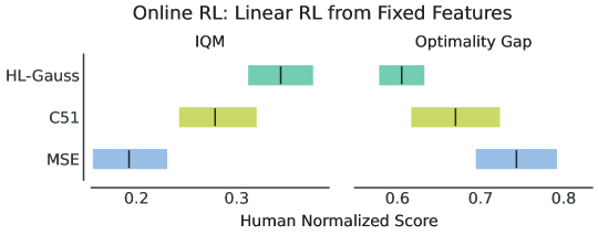
To investigate this question, following the protocol in Farebrother et al. (2023), we study whether a learned representation, corresponding to penultimate feature vectors, obtained from value-networks trained online on Atari for 200M frames, still retain the necessary information to re-learn a policy from scratch. To do so, we train a Q-function with a single linear layer on top of frozen representation (Farebrother et al., 2023), akin to how self-supervised representations are evaluated in vision (He et al., 2020). As shown in Figure 16, cross-entropy losses result in better performance with linear probing. This indicates that their learned representations are indeed better in terms of supporting the value-improvement path of a policy trained from scratch (Dabney et al., 2021).
5.2.3 Does Classification Perform Better Amidst Non-Stationarity?
Non-stationarity is inherent to value-based RL as the target computation involves a constantly evolving argmax policy and value function. Bellemare et al. (2017) hypothesized that classification might mitigate difficulty of learning from a non-stationary policy, but did not empirically validate it. Here, we investigate whether classification can indeed handle target non-stationarity better than regression.
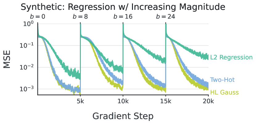
Synthetic setup: We first consider a synthetic regression task on CIFAR10 presented in Lyle et al. (2024), where the regression target corresponds to mapping an input image through a randomly initialized neural network to produce high-frequency targets where is a constant bias that can control for the magnitude of the targets. When learning a value function with TD, the prediction targets are non-stationary and often increase in magnitude over time as the policy improves. We simulate this setting by fitting a network with different losses on the increasing sequence of bias . See details in Appendix B.4. As shown in Figure 18, classification losses retain higher plasticity under non-stationary targets compared to regression.
Offline RL: To control non-stationarity in an RL context, we run offline SARSA, which estimates the value of the fixed data-collection policy, following the protcol in Kumar et al. (2022). Contrary to Q-learning, which use the action which maximizes the learned Q-value at the next state for computing the Bellman target (§2), SARSA uses the action observed at the next timestep in the offline dataset. As shown in Figure 18, most of the benefit from HL-Gauss compared to the MSE loss vanishes in the offline SARSA setting, adding evidence that some of the benefits from classification stem from dealing with non-stationarity in value-based RL.
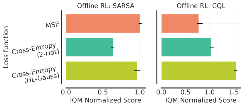
To summarize, we find that the use of cross-entropy loss itself is central to obtain good performance in value-based RL, and while these methods do not address any specific challenge, they enable value-based RL methods to deal better with non-stationarity, induce highly-expressive representations, and provide robustness against noisy target values.
6 Related Work
Prior works in tabular regression (Weiss and Indurkhya, 1995; Torgo and Gama, 1996) and computer vision (Van Den Oord et al., 2016; Kendall et al., 2017; Rothe et al., 2018; Rogez et al., 2019) have replaced regression with classification to improve performance. Most notably, Imani and White (2018) proposed the HL-Gauss cross-entropy loss for regression and show its efficacy on small-scale supervised regression tasks, outside of RL. Our work complements these prior works by illustrating for the first time that a classification objective trained with cross-entropy, particularly HL-Gauss, can enable effectively scaling for value-based RL on a variety of domains, including Atari, robotic manipulation, chess, and Wordle.
Several state-of-the-art methods in RL have used the Two-Hot cross-entropy loss without any analysis, either as an “ad-hoc” trick (Schrittwieser et al., 2020), citing benefits for sparse rewards (Hafner et al., 2023), or simply relying on folk wisdom (Hessel et al., 2021; Hansen et al., 2024). However, in our experiments, Two-Hot performs worse than other cross-entropy losses and MSE. We believe this is because Two-Hot does not effectively distribute probability to neighboring classes, unlike C51 and HL-Gauss (see §5.1.2 for an empirical investigation).
Closely related is the line of work on categorical distributional RL. Notably, Achab et al. (2023) offer an analysis of categorical one-step distributional RL, which corresponds precisely to the Two-Hot algorithm discussed herein with the similarity of these two approaches not being previously recognized. Additionally, the work of Bellemare et al. (2017) pioneered the C51 algorithm, and while their primary focus was not on framing RL as classification, our findings suggest that the specific loss function employed may play a more significant role in the algorithm’s success than modeling the return distribution itself. Several methods find that categorical distributional RL losses are important for scaling offline value-based RL (Kumar et al., 2023; Springenberg et al., 2024), but these works do not attempt to isolate which components of this paradigm are crucial for attaining positive scaling trends. We also note that these findings do not contradict recent theoretical work (Wang et al., 2023; Rowland et al., 2023) which argues that distributional RL brings statistical benefits over standard RL orthogonal to use of a cross entropy objective or the categorical representation.
Prior works have characterized the representations learned by TD-learning (Bellemare et al., 2019; Lyle et al., 2021; Le Lan et al., 2022, 2023; Kumar et al., 2021, 2022) but these prior works focus entirely on MSE losses with little to no work analyzing representations learned by cross-entropy based losses in RL. Our linear probing experiments in §5.2.2 try to fill this void, demonstrating that value-networks trained with cross-entropy losses learn better representations than regression. This finding is especially important since Imani and White (2018) did not find any representational benefits of HL-Gauss over MSE on supervised regression, indicating that the use of cross-entropy might have substantial benefits for TD-based learning methods in particular.
7 Conclusion
In this paper, we showed that framing regression as classification and minimizing categorical cross-entropy instead of the mean squared error yields large improvements in performance and scalability of value-based RL methods, on a wide variety of tasks, with several neural network architectures. We analyzed the source of these improvements and found that they stem specifically from the ability of the cross-entropy loss in enabling more expressive representations and handling noise and non-stationarity in value-based RL better. While the cross-entropy loss alone does not fully alleviate any of these problems entirely, our results show the substantial difference this small change can make.
We believe that strong results with the use categorical cross-entropy has implications for future algorithm design in deep RL, both in theory and practice. For instance, value-based RL approaches have been harder to scale and tune when the value function is represented by a transformer architecture and our results hint that classification might provide for a smooth approach to translate innovation in value-based RL to transformers. From a theoretical perspective, analyzing the optimization dynamics of cross-entropy might help devise improved losses or target distribution representations. Finally, while we did explore a number of settings, further work is required to evaluate the efficacy of classification losses in other RL problems such as those involving pre-training, fine-tuning, or continual RL.
Acknowledgements
We would like to thank Will Dabney for providing feedback on an early version of this paper. We’d also like to thank Clare Lyle, Mark Rowland, Marc Bellemare, Max Schwarzer, Pierluca D’oro, Nate Rahn, Harley Wiltzer, Wesley Chung, and Dale Schuurmans, for informative discussions. We’d also like to acknowledge Anian Ruoss, Grégoire Delétang, and Tim Genewein for their help with the Chess training infrastructure. This research was supported by the TPU resources at Google DeepMind, and the authors are grateful to Doina Precup and Joelle Baral for their support.
Author Contributions
JF led the project, implemented histogram-based methods, ran all the single-task online RL experiments on Atari, Q-distillation on Chess, jointly proposed and ran most of the analysis experiments, and contributed significantly to paper writing.
JO and AAT set up and ran the multi-task RL experiments and helped with writing. QV ran the robotic manipulation experiments and YC helped with the initial set-up. TX helped with paper writing and AI was involved in discussions. SL advised on the robotics and Wordle experiments and provided feedback. PSC helped set up the SoftMoE experiments and hosted Jesse at GDM. PSC and AF sponsored the project and took part in discussions.
AK advised the project, proposed offline RL analysis for non-stationarity and representation learning, contributed significantly to writing, revising, and the narrative, and set up the robotics and multi-game scaling experiments. RA proposed the research direction, advised the project, led the paper writing, ran offline RL and Wordle experiments, and helped set up all of the multi-task scaling and non-Atari experiments.
References
- Achab et al. (2023) Mastane Achab, Réda Alami, Yasser Abdelaziz Dahou Djilali, Kirill Fedyanin, and Eric Moulines. One-step distributional reinforcement learning. CoRR, abs/2304.14421, 2023.
- Agarwal et al. (2020) Rishabh Agarwal, Dale Schuurmans, and Mohammad Norouzi. An optimistic perspective on offline reinforcement learning. In International Conference on Machine Learning (ICML), 2020.
- Agarwal et al. (2021) Rishabh Agarwal, Max Schwarzer, Pablo Samuel Castro, Aaron Courville, and Marc G. Bellemare. Deep reinforcement learning at the edge of the statistical precipice. Neural Information Processing Systems (NeurIPS), 2021.
- Ali Taïga et al. (2023) Adrien Ali Taïga, Rishabh Agarwal, Jesse Farebrother, Aaron Courville, and Marc G. Bellemare. Investigating multi-task pretraining and generalization in reinforcement learning. In International Conference on Learning Representations (ICLR), 2023.
- Bellemare et al. (2013) Marc G. Bellemare, Yavar Naddaf, Joel Veness, and Michael Bowling. The arcade learning environment: An evaluation platform for general agents. Journal of Artificial Intelligence Research (JAIR), 47:253–279, 2013.
- Bellemare et al. (2017) Marc G. Bellemare, Will Dabney, and Rémi Munos. A distributional perspective on reinforcement learning. In International Conference on Machine Learning (ICML), 2017.
- Bellemare et al. (2019) Marc G. Bellemare, Will Dabney, Robert Dadashi, Adrien Ali Taïga, Pablo Samuel Castro, Nicolas Le Roux, Dale Schuurmans, Tor Lattimore, and Clare Lyle. A geometric perspective on optimal representations for reinforcement learning. In Neural Information Processing Systems (NeurIPS), 2019.
- Bellemare et al. (2023) Marc G. Bellemare, Will Dabney, and Mark Rowland. Distributional reinforcement learning. MIT Press, 2023.
- Bradbury et al. (2018) James Bradbury, Roy Frostig, Peter Hawkins, Matthew James Johnson, Chris Leary, Dougal Maclaurin, George Necula, Adam Paszke, Jake VanderPlas, Skye Wanderman-Milne, and Qiao Zhang. JAX: composable transformations of Python+NumPy programs, 2018. URL http://github.com/google/jax.
- Castro et al. (2018) Pablo Samuel Castro, Subhodeep Moitra, Carles Gelada, Saurabh Kumar, and Marc G. Bellemare. Dopamine: A Research Framework for Deep Reinforcement Learning. CoRR, abs/1812.06110, 2018.
- Ceron and Castro (2021) Johan Samir Obando Ceron and Pablo Samuel Castro. Revisiting rainbow: Promoting more insightful and inclusive deep reinforcement learning research. In International Conference on Machine Learning (ICML), 2021.
- Chebotar et al. (2023) Yevgen Chebotar, Quan Vuong, Karol Hausman, Fei Xia, Yao Lu, Alex Irpan, Aviral Kumar, Tianhe Yu, Alexander Herzog, Karl Pertsch, et al. Q-transformer: Scalable offline reinforcement learning via autoregressive q-functions. In Conference on Robot Learning (CoRL), 2023.
- Dabney et al. (2021) Will Dabney, André Barreto, Mark Rowland, Robert Dadashi, John Quan, Marc G. Bellemare, and David Silver. The value-improvement path: Towards better representations for reinforcement learning. In AAAI Conference on Artificial Intelligence, 2021.
- Espeholt et al. (2018) Lasse Espeholt, Hubert Soyer, Remi Munos, Karen Simonyan, Vlad Mnih, Tom Ward, Yotam Doron, Vlad Firoiu, Tim Harley, Iain Dunning, Shane Legg, and Koray Kavukcuoglu. Impala: Scalable distributed deep-rl with importance weighted actor-learner architectures. In International Conference on Machine Learning (ICML), 2018.
- Farebrother et al. (2018) Jesse Farebrother, Marlos C. Machado, and Michael Bowling. Generalization and regularization in DQN. CoRR, abs/1810.00123, 2018.
- Farebrother et al. (2023) Jesse Farebrother, Joshua Greaves, Rishabh Agarwal, Charline Le Lan, Ross Goroshin, Pablo Samuel Castro, and Marc G. Bellemare. Proto-value networks: Scaling representation learning with auxiliary tasks. In International Conference on Learning Representations (ICLR), 2023.
- Hafner et al. (2023) Danijar Hafner, Jurgis Pasukonis, Jimmy Ba, and Timothy P. Lillicrap. Mastering diverse domains through world models. CoRR, abs/2301.04104, 2023.
- Hansen et al. (2024) Nicklas Hansen, Hao Su, and Xiaolong Wang. TD-MPC2: Scalable, robust world models for continuous control. In International Conference on Learning Representations (ICLR), 2024.
- He et al. (2016) Kaiming He, Xiangyu Zhang, Shaoqing Ren, and Jian Sun. Deep residual learning for image recognition. In IEEE Conference on Computer Vision and Pattern Recognition (CVPR), 2016.
- He et al. (2020) Kaiming He, Haoqi Fan, Yuxin Wu, Saining Xie, and Ross Girshick. Momentum contrast for unsupervised visual representation learning. In IEEE Conference on Computer Vision and Pattern Recognition (CVPR), 2020.
- Hessel et al. (2021) Matteo Hessel, Ivo Danihelka, Fabio Viola, Arthur Guez, Simon Schmitt, Laurent Sifre, Theophane Weber, David Silver, and Hado van Hasselt. Muesli: Combining improvements in policy optimization. In International Conference on Machine Learning (ICML), 2021.
- Ho et al. (2021) Daniel Ho, Kanishka Rao, Zhuo Xu, Eric Jang, Mohi Khansari, and Yunfei Bai. Retinagan: An object-aware approach to sim-to-real transfer. In IEEE International Conference on Robotics and Automation (ICRA), 2021.
- Imani and White (2018) Ehsan Imani and Martha White. Improving regression performance with distributional losses. In International Conference on Machine Learning (ICML), 2018.
- Imani et al. (2024) Ehsan Imani, Kai Luedemann, Sam Scholnick-Hughes, Esraa Elelimy, and Martha White. Investigating the histogram loss in regression. CoRR, abs/2402.13425, 2024.
- Kaplan et al. (2020) Jared Kaplan, Sam McCandlish, Tom Henighan, Tom B Brown, Benjamin Chess, Rewon Child, Scott Gray, Alec Radford, Jeffrey Wu, and Dario Amodei. Scaling laws for neural language models. CoRR, abs/2001.08361, 2020.
- Kendall et al. (2017) Alex Kendall, Hayk Martirosyan, Saumitro Dasgupta, Peter Henry, Ryan Kennedy, Abraham Bachrach, and Adam Bry. End-to-end learning of geometry and context for deep stereo regression. In IEEE International Conference on Computer Vision (ICCV), 2017.
- Krizhevsky et al. (2012) Alex Krizhevsky, Ilya Sutskever, and Geoffrey E Hinton. Imagenet classification with deep convolutional neural networks. Neural Information Processing Systems (NeurIPS), 2012.
- Kumar et al. (2020) Aviral Kumar, Aurick Zhou, George Tucker, and Sergey Levine. Conservative q-learning for offline reinforcement learning. Neural Information Processing Systems (NeurIPS), 2020.
- Kumar et al. (2021) Aviral Kumar, Rishabh Agarwal, Dibya Ghosh, and Sergey Levine. Implicit under-parameterization inhibits data-efficient deep reinforcement learning. In International Conference on Learning Representations (ICLR), 2021.
- Kumar et al. (2022) Aviral Kumar, Rishabh Agarwal, Tengyu Ma, Aaron Courville, George Tucker, and Sergey Levine. Dr3: Value-based deep reinforcement learning requires explicit regularization. In International Conference on Learning Representations (ICLR), 2022.
- Kumar et al. (2023) Aviral Kumar, Rishabh Agarwal, Xinyang Geng, George Tucker, and Sergey Levine. Offline Q-Learning on Diverse Multi-Task Data Both Scales and Generalizes. In International Conference on Learning Representations (ICLR), 2023.
- Le Lan et al. (2022) Charline Le Lan, Stephen Tu, Adam Oberman, Rishabh Agarwal, and Marc G. Bellemare. On the generalization of representations in reinforcement learning. In International Conference on Artificial Intelligence and Statistics (AISTATS), 2022.
- Le Lan et al. (2023) Charline Le Lan, Stephen Tu, Mark Rowland, Anna Harutyunyan, Rishabh Agarwal, Marc G. Bellemare, and Will Dabney. Bootstrapped representations in reinforcement learning. In International Conference on Machine Learning (ICML), 2023.
- Lee et al. (2022) Kuang-Huei Lee, Ofir Nachum, Mengjiao (Sherry) Yang, Lisa Lee, Daniel Freeman, Sergio Guadarrama, Ian Fischer, Winnie Xu, Eric Jang, Henryk Michalewski, and Igor Mordatch. Multi-game decision transformers. In Neural Information Processing Systems (NeurIPS), 2022.
- Lehnert et al. (2024) Lucas Lehnert, Sainbayar Sukhbaatar, Paul Mcvay, Michael Rabbat, and Yuandong Tian. Beyond a*: Better planning with transformers via search dynamics bootstrapping. CoRR, abs/2402.14083, 2024.
- Levine et al. (2020) Sergey Levine, Aviral Kumar, George Tucker, and Justin Fu. Offline Reinforcement Learning: Tutorial, Review, and Perspectives on Open Problems. CoRR, abs/2005.01643, 2020.
- Lyle et al. (2019) Clare Lyle, Marc G. Bellemare, and Pablo Samuel Castro. A comparative analysis of expected and distributional reinforcement learning. In AAAI Conference on Artificial Intelligence, 2019.
- Lyle et al. (2021) Clare Lyle, Mark Rowland, Georg Ostrovski, and Will Dabney. On the effect of auxiliary tasks on representation dynamics. In International Conference on Artificial Intelligence and Statistics (AISTATS), 2021.
- Lyle et al. (2022) Clare Lyle, Mark Rowland, and Will Dabney. Understanding and preventing capacity loss in reinforcement learning. In International Conference on Learning Representations (ICLR), 2022.
- Lyle et al. (2024) Clare Lyle, Zeyu Zheng, Khimya Khetarpal, Hado van Hasselt, Razvan Pascanu, James Martens, and Will Dabney. Disentangling the causes of plasticity loss in neural networks. CoRR, abs/2402.18762, 2024.
- Machado et al. (2018) Marlos C. Machado, Marc G. Bellemare, Erik Talvitie, Joel Veness, Matthew Hausknecht, and Michael Bowling. Revisiting the arcade learning environment: Evaluation protocols and open problems for general agents. Journal of Artificial Intelligence Research (JAIR), 61:523–562, 2018.
- Mnih et al. (2015) Volodymyr Mnih, Koray Kavukcuoglu, David Silver, Andrei A. Rusu, Joel Veness, Marc G. Bellemare, Alex Graves, Martin Riedmiller, Andreas K. Fidjeland, Georg Ostrovski, Stig Petersen, Charles Beattie, Amir Sadik, Ioannis Antonoglou, Helen King, Dharshan Kumaran, Daan Wierstra, Shane Legg, and Demis Hassabis. Human-level control through deep reinforcement learning. Nature, 518(7540):529–533, 2015.
- Mnih et al. (2016) Volodymyr Mnih, Adria Puigdomenech Badia, Mehdi Mirza, Alex Graves, Timothy Lillicrap, Tim Harley, David Silver, and Koray Kavukcuoglu. Asynchronous methods for deep reinforcement learning. In International Conference on Machine Learning (ICML), 2016.
- Obando-Ceron et al. (2024) Johan Obando-Ceron, Ghada Sokar, Timon Willi, Clare Lyle, Jesse Farebrother, Jakob Foerster, Gintare Karolina Dziugaite, Doina Precup, and Pablo Samuel Castro. Mixtures of experts unlock parameter scaling for deep rl. CoRR, abs/2402.08609, 2024.
- Paszke et al. (2019) Adam Paszke, Sam Gross, Francisco Massa, Adam Lerer, James Bradbury, Gregory Chanan, Trevor Killeen, Zeming Lin, Natalia Gimelshein, Luca Antiga, Alban Desmaison, Andreas Kopf, Edward Yang, Zachary DeVito, Martin Raison, Alykhan Tejani, Sasank Chilamkurthy, Benoit Steiner, Lu Fang, Junjie Bai, and Soumith Chintala. Pytorch: An imperative style, high-performance deep learning library. In Neural Information Processing Systems (NeurIPS), 2019.
- Pintea et al. (2023) Silvia L. Pintea, Yancong Lin, Jouke Dijkstra, and Jan C. van Gemert. A step towards understanding why classification helps regression. In IEEE International Conference on Computer Vision (ICCV), pages 19972–19981, 2023.
- Puigcerver et al. (2024) Joan Puigcerver, Carlos Riquelme Ruiz, Basil Mustafa, and Neil Houlsby. From sparse to soft mixtures of experts. In International Conference on Learning Representations (ICLR), 2024.
- Rogez et al. (2019) Gregory Rogez, Philippe Weinzaepfel, and Cordelia Schmid. Lcr-net++: Multi-person 2d and 3d pose detection in natural images. IEEE Transactions on Pattern Analysis and Machine Intelligence (PAMI), 42(5):1146–1161, 2019.
- Rothe et al. (2018) Rasmus Rothe, Radu Timofte, and Luc Van Gool. Deep expectation of real and apparent age from a single image without facial landmarks. International Journal of Computer Vision (IJCV), 126(2-4):144–157, 2018.
- Rowland et al. (2023) Mark Rowland, Yunhao Tang, Clare Lyle, Rémi Munos, Marc G. Bellemare, and Will Dabney. The statistical benefits of quantile temporal-difference learning for value estimation. In International Conference on Machine Learning (ICML), 2023.
- Ruoss et al. (2024) Anian Ruoss, Grégoire Delétang, Sourabh Medapati, Jordi Grau-Moya, Li Kevin Wenliang, Elliot Catt, John Reid, and Tim Genewein. Grandmaster-level chess without search. CoRR, abs/2402.04494, 2024.
- Schrittwieser et al. (2020) Julian Schrittwieser, Ioannis Antonoglou, Thomas Hubert, Karen Simonyan, Laurent Sifre, Simon Schmitt, Arthur Guez, Edward Lockhart, Demis Hassabis, Thore Graepel, Timothy P. Lillicrap, and David Silver. Mastering atari, go, chess and shogi by planning with a learned model. Nature, 588(7839):604–609, 2020.
- Silver et al. (2017) David Silver, Julian Schrittwieser, Karen Simonyan, Ioannis Antonoglou, Aja Huang, Arthur Guez, Thomas Hubert, Lucas Baker, Matthew Lai, Adrian Bolton, Yutian Chen, Timothy Lillicrap, Fan Hui, Laurent Sifre, George van den Driessche, Thore Graepel, and Demis Hassabis. Mastering the game of go without human knowledge. Nature, 550(7676):354–359, 2017.
- Snell et al. (2023) Charlie Victor Snell, Ilya Kostrikov, Yi Su, Sherry Yang, and Sergey Levine. Offline RL for natural language generation with implicit language q learning. In International Conference on Learning Representations (ICLR), 2023.
- Springenberg et al. (2024) Jost Tobias Springenberg, Abbas Abdolmaleki, Jingwei Zhang, Oliver Groth, Michael Bloesch, Thomas Lampe, Philemon Brakel, Sarah Bechtle, Steven Kapturowski, Roland Hafner, et al. Offline actor-critic reinforcement learning scales to large models. CoRR, abs/2402.05546, 2024.
- Stewart et al. (2023) Lawrence Stewart, Francis Bach, Quentin Berthet, and Jean-Philippe Vert. Regression as classification: Influence of task formulation on neural network features. In International Conference on Artificial Intelligence and Statistics (AISTATS), 2023.
- Szegedy et al. (2016) Christian Szegedy, Vincent Vanhoucke, Sergey Ioffe, Jonathon Shlens, and Zbigniew Wojna. Rethinking the inception architecture for computer vision. In IEEE Conference on Computer Vision and Pattern Recognition (CVPR), 2016.
- Torgo and Gama (1996) Luís Torgo and João Gama. Regression by classification. In Brazilian Symposium on Artificial Intelligence, pages 51–60. Springer, 1996.
- Van Den Oord et al. (2016) Aäron Van Den Oord, Nal Kalchbrenner, and Koray Kavukcuoglu. Pixel recurrent neural networks. In International Conference on Machine Learning (ICML), 2016.
- Vaswani et al. (2017) Ashish Vaswani, Noam Shazeer, Niki Parmar, Jakob Uszkoreit, Llion Jones, Aidan N Gomez, Łukasz Kaiser, and Illia Polosukhin. Attention is all you need. Neural Information Processing Systems (NeurIPS), 2017.
- Wang et al. (2023) Kaiwen Wang, Kevin Zhou, Runzhe Wu, Nathan Kallus, and Wen Sun. The benefits of being distributional: Small-loss bounds for reinforcement learning. In Neural Information Processing Systems (NeurIPS), 2023.
- Weiss and Indurkhya (1995) Sholom M Weiss and Nitin Indurkhya. Rule-based machine learning methods for functional prediction. Journal of Artificial Intelligence Research (JAIR), 3:383–403, 1995.
- Zhang et al. (2023) Shihao Zhang, Linlin Yang, Michael Bi Mi, Xiaoxu Zheng, and Angela Yao. Improving deep regression with ordinal entropy. In International Conference on Learning Representations (ICLR), 2023.
Appendix A Reference Implementations
Appendix B Experimental Methodology
In the subsequent sections we outline the experimental methodology for each domain herein.
B.1 Atari
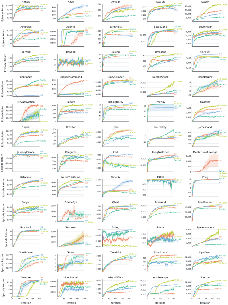
Both our online and offline RL regression baselines are built upon the Jax (Bradbury et al., 2018) implementation of DQN+Adam in Dopamine (Castro et al., 2018). Similarly, each of the classification methods (i.e., HL-Gauss and Two-Hot) were built upon the Jax (Bradbury et al., 2018) implementation of C51 in Dopamine (Castro et al., 2018). Hyperparameters for DQN+Adam are provided in Table B.3 along with any hyperparameter differences for C51 (Table B.3), Two-Hot (Table B.3), and HL-Gauss (Table B.3). Unless otherwise stated the online RL results in the paper were ran for 200M frames on 60 Atari games with five seeds per game. The offline RL results were ran on the 17 games in Kumar et al. (2021) with three seeds per game. The network architecture for both the online and offline results is the standard DQN Nature architecture that employs three convolutional layers followed by a single non-linear fully-connected layer before outputting the action-values.
| Discount Factor | 0.99 |
|---|---|
| -step | 1 |
| Minimum Replay History | agent steps |
| Agent Update Frequency | environment steps |
| Target Network Update Frequency | agent steps |
| Exploration | |
| Exploration decay | agent steps |
| Optimizer | Adam |
| Learning Rate | |
| Adam | |
| Sticky Action Probability | |
| Maximum Steps per Episode | agent steps |
| Replay Buffer Size | |
| Batch Size |
B.1.1 Mixtures of Experts
All experiments ran with SoftMoE reused the experimental methodology of Obando-Ceron et al. (2024). Specifically, we replace the penultimate layer of the DQN+Adam in Dopamine (Castro et al., 2018) with a SoftMoE (Puigcerver et al., 2024) module. The MoE results were ran with the Impala ResNet architecture (Espeholt et al., 2018). We reuse the same set of games from Obando-Ceron et al. (2024) and run each configuration for five seeds per game. All classification methods reused the parameters from Table B.3 for C51 and Two-Hot or Table B.3 for HL-Gauss.
B.1.2 Multi-Task & Multi-Game
The multi-task and multi-game results follow exactly the methodology outlined in Ali Taïga et al. (2023) and Kumar et al. (2023) respectively. We reuse the hyperparameters for HL-Gauss outlined in Table B.3. For multi-task results each agent is run for five seeds per game. Due to the prohibitive compute of the multi-game setup we run each configuration for a single seed.
B.2 Chess
We follow exactly the setup in Ruoss et al. (2024) with the only difference being the use of HL-Gauss with a smoothing ratio . Specifically, we take the action-values produced by Stockfish and project them a categorical distribution using HL-Gauss. As Ruoss et al. (2024) was already performing classification we reuse the parameters of their categorical distribution, those being, bins evenly divided between the range . For each parameter configuration we train a single agent and report the evaluation puzzle accuracy. Puzzle accuracy numbers for one-hot and AlphaZero w/ MCTS were taken directly from Ruoss et al. (2024, Table 6).
B.3 Robotic manipulation experiments.
We study a large-scale vision-based robotic manipulation setting on a mobile manipulator robot with 7 degrees of freedom, which is visualized in Figure 10 (left). The tabletop robot manipulation domain consists of a tabletop with various randomized objects spawned on top of the countertop. A RetinaGAN is applied to transform the simulation images closer to real-world image distributions, following the method in (Ho et al., 2021). We implement a Q-Transformer policy following the procedures in (Chebotar et al., 2023). Specifically, we incorporate autoregressive -learning by learning -values per action dimension, incorporate conservative regularization to effectively learn from suboptimal data, and utilize Monte-Carlo returns.

B.4 Regression Target Magnitude & Loss of Plasticity
To assess whether classification losses are more robust when learning non-stationary targets of increasing magnitude we leverage the synthetic setup from Lyle et al. (2024). Specifically, we train a convolutional neural network that takes CIFAR 10 images as input and outputs a scalar prediction: . The goal is to fit the regression target,
where , are a set of randomly sampled target parameters for the same convolutional architecture, and is a bias that changes the magnitude of the prediction targets. It is clear that increasing shouldn’t result in a more challenging regression task.
When learning a value function with TD methods the regression targets are non-stationary and hopefully increasing in magnitude (corresponding to an improving policy). To simulate this setting we consider fitting the network on the increasing sequence . For each value we sample a new set of target parameters and regress towards for gradient steps with a batch size of with the Adam optimizer using a learning rate of .
We evaluate the Mean-Squared Error (MSE) throughout training for three methods: Two-Hot, HL-Gauss, and L2 regression. For both Two-Hot and HL-Gauss we use a support of with bins. Figure 18 depicts the MSE throughout training averaged over seeds for each method. One can see that the network trained with L2 regression does indeed loose its ability to rapidly fit targets of increasing magnitude, consistent with Lyle et al. (2024). On the other hand, the classification methods are more robust and tend to converge to the same MSE irrespective of the target magnitude . Furthermore, we can see that HL-Gauss outperforms Two-Hot, consistent with our previous findings. These results help provide some evidence that perhaps one of the reasons classification outperforms regression is due to the network being more “plastic” under non-stationary targets.
Appendix C Per-Game Atari Results
Appendix D Additional Results
